Admissibility in partial conjunction testing

Abstract

Meta-analysis combines results from multiple studies aiming to increase power in finding their common effect. It would typically reject the null hypothesis of no effect if any one of the studies shows strong significance. The partial conjunction null hypothesis is rejected only when at least $r$ of $n$ component hypotheses are non-null with $r=1$ corresponding to a usual meta-analysis. Compared with meta-analysis, it can encourage replicable findings across studies. A by-product of it when applied to different $r$ values is a confidence interval of $r$ quantifying the proportion of non-null studies. Benjamini and Heller (2008) provided a valid test for the partial conjunction null by ignoring the $r-1$ smallest p-values and applying a valid meta-analysis p-value to the remaining $n-r+1$ p-values. We provide sufficient and necessary conditions of admissible combined p-value for the partial conjunction hypothesis among monotone tests. Non-monotone tests always dominate monotone tests but are usually too unreasonable to be used in practice. Based on these findings, we propose a generalized form of Benjamini and Heller’s test which allows usage of various types of meta-analysis p-values, and apply our method to an example in assessing replicable benefit of new anticoagulants across subgroups of patients for stroke prevention.

1 Introduction

When a null hypothesis is tested in $n$ different settings, a meta-analysis can be used to obtain a combined p-value based on all of the test results. It gains power as the combined p-value is usually more significant than any of the individual p-value in each setting. However, the combined p-value in meta-analysis is only valid for the global null where the null hypothesis is true in every setting, thus it is possible that the null is then rejected largely on the basis of just one extremely significant component hypothesis test. Such a rejection may be undesirable as it could arise from some irreproducible property of the setting in which that one component test was made.

Table 1: four hypothetical cases for five ordered p-values.

Case	$p_{(1)}$	$p_{(2)}$	$p_{(3)}$	$p_{(4)}$	$p_{(5)}$
A	$10^{-200}$	$0.4$	$0.5$	$0.6$	$0.7$
B	$10^{-10}$	$10^{-9}$	$10^{-8}$	$10^{-7}$	$10^{-6}$
C	$10^{-100}$	$10^{-100}$	$10^{-100}$	$0.049$	$0.8$
D	$0.048$	$0.048$	$0.048$	$0.048$	$0.8$

Refering to Table 1, cases A and B illustrate the potential problem of meta-analysis. Both a Fisher and a Stouffer meta-analysis would find case A more significant than case B, while the only significant setting in case A may largely due to a technical or statistical bias. The random effect model in meta-analysis has been widely accepted for consideration of heteogeneity across studies (Higgins et al., 2009). However, it still assumes that the effects across studies are similar and does not explicitly guarantee replication nor being robust to extreme bias.

Researchers in functional magnetic resonance imaging (fMRI) have adopted conjunction (logical ‘and’) testing (Price and Friston, 1997; Friston et al., 1999; Nichols et al., 2005) in which a hypothesis must be rejected in all $n$ settings where it is tested. The $n$ settings may correspond to related tasks or they may correspond to independent subjects. For example in Table 1, a conjunction test would only reject case B which shows consistent replication. However, conjunction tests lose power for large $n$ as they are based on the largest of $n$ p-values. A compromise is to require evidence that at least $r$ out of $n$ null hypotheses are false, for some user specified $r$. Such tests of the ‘partial conjunction (PC) null hypothesis’ were used in Friston et al. (2005) and then studied by Benjamini and Heller (2008). The extremes $r=1$ and $r=n$ correspond to the usual meta-analysis tests and conjunction testing respectively.

Partial conjunction testing is useful in areas beyond neuroimaging. It is the tool for replicability analysis, which finds effects that present in more than one studies, and has been applied in systematic review for healthcare prevention (Shenhav et al., 2015) and genome-wide association studies (Heller et al., 2014). PC test also has the potential usage in finding common gene regulation patterns across tissues for eQTL data (Flutre et al., 2013). Besides, it can be applied to gene set enrichment analysis to avoid selection of gene sets whose significance depend on only one single gene (Wang et al., 2010).

A Benjamini-Heller partial conjunction (BHPC) test works as follows. One sorts the observed p-values yielding $p_{(1)}\leq p_{(2)}\leq\dots\leq p_{(n)}$, ignores the smallest $r-1$ of them, and then applies a valid p-value combination rule to the remaining $n-r+1$ p-values. Benjamini and Heller (2008) show that BHPC tests are valid for the partial conjunction null when the $n$ hypotheses are independent. They also consider some dependent test conditions as well as the consequences of using PC tests in the Benjamini-Hochberg procedure.

Cases C and D illustrate an interesting property of the BHPC tests. Suppose that we need to reject at least four null hypotheses to have a meaningful finding. Then a BHPC test finds that case D is stronger evidence (smaller p-value) than case C, because BHPC is based only on $p_{(4)}$ and $p_{(5)}$. In case C we are extremely confident of three rejections and are banking on the fourth one to be correct. In case D by contrast, none of the four smallest p-values is much better than borderline. It appears to have about four times as many ways to disappointing us. This comparsion between case C and D reveals a counter-intuitive property of the BHPC tests, that we study further.

Here we investigate the power properties of BHPC tests focussing on admissibility. Under the assumption that the component p-values are either independent or have a positive dependency structure, we characterize the complete class of tests for monotone admissibility, which is a generalized form of BHPC p-values (GBHPC p-values). the only admissible PC tests among monotone tests are either of the BHPC form, or its generalization (GBHPC), which uses combined p-values constructed by taking the maximum of the meta-analysis p-value of each of the $n\choose{r-1}$ subsets of $n-r+1$ hypotheses. Under mild assumptions, a sufficient condition for the monotone admissibility of a GBHPC p-value is that each of the meta-analysis p-value for $n\choose{r-1}$ subsets is admissible. GBHPC p-values are also called r-values in Shenhav et al. (2015).

The monotonicity condition, which means that the combined p-value is a non-decreasing function of the individual p-values, is necessary for us to discuss admissibility for partial conjunction hypotheses with $r>1$. If we relax this condition, then BHPC tests become inadmissible. Because non-monotone tests are quite unreasonable scientifically in most cases, this is not a strong criticism of BHPC. We side with Perlman and Wu (1999) in rejecting the admissibility criterion not the test, when methods lacking face-value validity are included in comparisons.

The admissibility properties show supreme of BHPC p-values, but how can we then explain its puzzling behavior alluded to for cases C and D in Table 1? An explanation is that unlike the combined p-values in meta-analysis, the PC p-values measure the strength of replicability (the true proportion of non-null studies) instead of the magnitude of effect size. a PC p-value can be much smaller when the true number ($r_{0}$) rather than the effect size of non-null studies is large. Compared with case D, the three extreme p-values of case C in Table 1 gain us much stronger evidence of a large effect size but not much more evidence on $r_{0}\geq 4$. Thus, the PC p-values for both case C and case D are similar.

Section 2 presents our notation and some background on partial conjunction tests and admissibility. Section 3 proposes the GBHPC p-values and presents the main theorems on monotone admissible partial conjunction p-values. Section 4 is a simulation study for the power comparison of several GBHPC p-values under various hypotheses configurations. Compared with BHPC p-values, GBHPC p-values have the advantage that it can be constructed from more sophisticated meta-analysis p-values. We illustrate this benefit in Section 5 in an application of GBHPC p-values for assessing replicable benefit and safety concerns of new oral anticoagulants across subgroups of patients for stroke prevention. Section 6 has our conclusions and states some future work.

2 Preliminaries

2.1 Definitions and notations

The problem begins with $n$ null hypotheses to test, $H_{0i}$ for $i=1,\dots,n$. Each $H_{0i}$ is the hypothesis to test for an individual setting/study. The corresponding alternative hypotheses are $H_{1i}$. The $i$’th hypothesis refers to a parameter $\theta_{i}$. If $H_{0i}$ holds then $\theta_{i}\in\Theta_{0i}$, while $H_{1i}$ specifies that $\theta_{i}\in\Theta_{1i}$. The parameter space for the $i$’th hypothesis is $\Theta_{i}=\Theta_{0i}\cup\Theta_{1i}$ and of course $\Theta_{0i}\cap\Theta_{1i}=\varnothing$. The parameter space of $(\theta_{1},\dots,\theta_{n})$ is $\Theta=\prod_{i}\Theta_{i}$.

To each hypothesis, there corresponds a p-value, $p_{i}$. there may be a loss of information in reducing a data set to one p-value. Yet often that loss is small and very commonly the researchers who gathered the original data share only their p-values for reasons that may include privacy of their subjects.

We use $p_{i}$ to denote the numerical value of the p-value for the $i$’th hypothesis. It is the observed value of a corresponding random variable $P_{i}$. The sorted p-values are $p_{(1)}\leq p_{(2)}\leq\dots\leq p_{(n)}$ and $P_{(1)}\leq P_{(2)}\leq\dots\leq P_{(n)}$ are the sorted random variables. Probability and expectation for functions of $P_{i}$ are given by $\mathbb{P}_{\theta_{i}}$ and $\mathbb{E}_{\theta_{i}}$ respectively. We let $\theta=(\theta_{1},\dots,\theta_{n})$ and $\bm{P}=(P_{1},\dots,P_{n})$. Probability and expectation for functions of $\bm{P}$ are given by $\mathbb{P}_{\theta}$ and $\mathbb{E}_{\theta}$. Each $p_{i}$ is a valid P-value according to the definition below:

Definition 1 (Validity).

A valid component p-value satisfies $\sup_{\theta_{i}\in\Theta_{0i}}\mathbb{P}_{\theta_{i}}(P_{i}\leq\alpha)\leq\alpha$ for $0\leq\alpha\leq 1$.

Besides independency, positive dependency can be a common dependency structure across studies, especially when they share samples. For $P_{1},\dots,P_{n}$, we assume that they are either independent or positively dependent (PRDS) (Benjamini and Yekutieli, 2001) Under any parameter $\theta\in\Theta$. Using the definition of PRDS thus they have the following property: for $\forall(p_{1},\cdots,p_{n})\in[0,1]^{n}$ and $\forall\theta\in\Theta$,

$$\mathbb{P}_{\theta}(P_{1}\leq p_{1},\cdots,P_{n}\leq p_{n})\geq\prod_{i}\mathbb{P}_{\theta_{i}}(P_{i}\leq p_{i})$$ (1)

For a given $r\leq n$, the PC null hypothesis and alternative hypothesis are defined as

$$H_{0}^{r/n}:\quad \{\text{at most }r-1\text{ hypotheses are non-null}\},\quad\text{and}$$

$$H_{1}^{r/n}:\quad \{\text{at least }r\text{ hypotheses are non-null}\}.$$

The null space is defined as $\Theta_{0}^{r/n}=\{\theta\in\Theta:H_{0}^{r/n}\text{ is true}\}$.

We use $1{:}r$ to denote $\{1,2,\dots,r\}$ and similarly $(r+1){:}n=\{r+1,r+2,\dots,n\}$. The index set $u\subset 1{:}n$ has cardinality $|u|$ and complement $-u=1{:}n\setminus u$. Under the null hypothesis $H_{0u}$ we have $\theta_{j}\in\Theta_{0j}$ for all $j\in u$. The null space of $H_{0u}$ is denoted as $\Theta_{0u}$.

Sometimes we combine points $\bm{x}\in\mathbb{R}^{n}$ and $\bm{y}\in\mathbb{R}^{n}$ into a point $\bm{z}\in\mathbb{R}^{n}$ with $z_{j}=x_{j}$ for $j\in u$ and $z_{j}=y_{j}$ for $j\not\in u$. Such a hybrid point is denoted $\bm{z}=\bm{x}_{u}{:}\bm{y}_{-u}$. Let $u=\{i_{1},i_{2},\dots,i_{k}\}$, then $\theta_{u}$ is defined as the combination $(\theta_{i_{1}},\theta_{i_{2}},\dots,\theta_{i_{k}})$.

We can extend the definition of validity to meta-analysis and PC p-values. The combination of $k$ p-values ($k$ may differ from $n$ later) produces the combined p-value $p_{r/k}=f_{r,k}(P_{1},\dots,P_{k})$ which is a valid p-value for testing $H_{0}^{r/k}$ if

$$\sup_{\theta\in\Theta_{0}^{r/n}}\mathbb{P}_{\theta}(P_{r/k}\leq\alpha)\leq\alpha,\quad\forall\,0\leq\alpha\leq 1.$$

Definition 2 (Sensitivity).

A sensitive p-value $P_{r/k}=f_{r,k}(P_{1},\dots,P_{k})$ for $H_{0}^{r/n}$ satisfies

$$\liminf_{\bm{P}_{u}\to\bm{0}}P_{r/k}=0$$

for $\forall u\subset 1{:}k$ and $|u|=r$.

Sensitivity requires that PC p-value drops to $0$ when we are certain to reject any of $r$ individual hypotheses. For meta-analysis p-value $P_{1/k}$, it means that we reject the global null when we are certain at any of the individual hypothesis. We think that it is a practically reasonable requirement for a p-value for testing $H_{0}^{r/k}$.

Here are some examples of valid and sensitive meta-analysis p-values given valid p-values $p_{1},\dots,p_{k}$. The combination for a method $M$ is defined in terms of a function $f_{M,k}$ which may incorporate sorting of its arguments.

Example 1.

Simes’ method:

$$p_{S,k}=f_{S,k}(p_{1},\dots,p_{k})\equiv\min_{i=1,\cdots,k}\biggl{\{}\frac{kp_{(i)}}{i}\biggr{\}}.$$

Example 2.

Fisher’s method:

$$p_{F,k}=f_{F,k}(p_{1},\dots,p_{k})\equiv\mathbbm{P}\biggl{(}\chi_{(2k)}^{2}\geq-2\sum_{i=1}^{k}\log p_{i}\biggr{)}.$$

Example 3.

Weighted Stouffer test: Consider test statistics $T_{i}\sim\mathcal{N}(\sqrt{n_{i}}\theta_{i}/\sigma_{i},1)$, with sample sizes $n_{i}$ for $i=1,\dots,k$ and known $\sigma_{i}>0$. The p-value for the null that $\theta_{i}=0$ versus the alternative that $\theta_{i}>0$ is $p_{i}=1-\Phi(T_{i})=\Phi(-T_{i})$. A weighted Stouffer p-value for $H_{0}^{1/k}$ takes the form

$$p_{\mathrm{WS},k}=p_{\mathrm{WS},k}(p_{1},\dots,p_{k})\equiv 1-\Phi\Biggl{(}\frac{\sum_{i=1}^{k}\sqrt{n_{i}}\Phi^{-1}(1-p_{i})/\sigma_{i}}{\sqrt{\sum_{i=1}^{k}{n_{i}}/\sigma_{i}^{2}}}\Biggr{)}.$$

In fact, $p_{\mathrm{WS},k}$ can be used beyond one-sided tests. For example, for two-sided test $\Phi^{-1}(1-p_{i})$ also has the magnitude roughly proportional to $\sqrt{n_{i}}$. We shall illustrate the performance under such usage in our simulations in Section 4.

Example 4.

Truncated product method (Zaykin et al., 2002): this is a more recently developed method to gain efficiency in the presence of outliers. The test statistic has the form

$$w_{\gamma}=\prod_{i}p_{i}^{1_{p_{i}\leq\gamma}}$$

where $\gamma$ is some pre-determined value. The TPM p-value for $H_{0}^{1/k}$ takes the form

$$p_{\mathrm{TPM},k}=\mathbb{P}(W\leq w_{\gamma}).$$

where the probability function of $W$ was computed for both independency and dependent scenarios in (Zaykin et al., 2002).

For non-symmetric meta-analysis p-values, there are also weighted versions of Fisher tests. Note that each of the functions $f$ in the previous examples is monotone according to this definition:

Definition 3.

(Monotonicity) the p-value $f(p_{1},\dots,p_{k})$ is monotone if the function $f$ is non-decreasing in each argument. The set of such monotone p-value functions is denoted $\mathcal{F}_{\mathrm{mon}}$. a monotone test is one that rejects its null hypothesis for small values of a monotone p-value.

A non-monotone test would reject its null hypothesis at some input $(p_{1},\dots,p_{k})$ but fail to reject at some $(p_{1}^{\prime},\dots,p_{k}^{\prime})$ with all $p_{i}^{\prime}\leq p_{i}$. Such a test is typically unreasonable.

Besides monotonicity, we also clearify the definition of a symmetric combined p-value:

Definition 4.

(Symmetry) The combined p-value $f(p_{1},\dots,p_{k})$ is symmetric if its value stays unchanged under any permutation of $\{p_{1},\dots,p_{k}\}$.

Finally, we state the concept of admissibility using the definition of admissible tests from Lehmann and Romano (2006, Chapter 6.7). Let a hypothesis test of $H_{0}$ versus $H_{1}$ described by a function $\varphi(X)\in\{0,1\}$ of the data $X$. If $\varphi(X)=1$ then $H_{0}$ is rejected and $\varphi(X)=0$ otherwise. The test $\varphi$ is valid at level $\alpha$ if $\sup_{\theta\in\Theta_{0}}\mathbb{E}_{\theta}(\varphi(X))\leq\alpha$. In our context, the data are a vector $\bm{P}=(P_{1},\dots,P_{n})$ of p-values and $\varphi(P_{1},\dots,P_{n})=1_{f(P_{1},\dots,P_{n})\leq\alpha}$ where $f$ is a p-value combination function.

Definition 5 ($\Psi$,$\alpha$-admissibility).

The level-$\alpha$ test $\varphi\in\Psi$ is $\alpha$-admissible for testing $H_{0}:\theta\in\Theta_{0}$ against $H_{1}:\theta\in\Theta_{1}$ if for any other level-$\alpha$ test $\varphi^{\prime}\in\Psi$

$$\mathbb{E}_{\theta}(\varphi^{\prime})\geq\mathbb{E}_{\theta}(\varphi),\quad\text{for all $\theta\in\Theta_{1}$}$$

implies $\mathbb{E}_{\theta}(\varphi^{\prime})=\mathbb{E}_{\theta}(\varphi)$ for all $\theta\in\Theta_{1}$.

The definition of admissibility depends on the alternatives in $\Theta_{1}$ as well as the space $\Psi$ of test functions. The constraints on $\Theta_{1}$ are important. for the ordinary meta-analysis, Birnbaum (1954) shows that every monotone p-value is admissible when the component p-values are independent and the null hypothesis is simple, because there is then some alternative at which that p-value gives optimal power. However, those optimizing alternatives may not all be reasonable. Birnbaum (1955) and Stein (1956) (generalized later by Matthes and Truax (1967) to include nuisance parameters) also showed that for the ordinary meta-analysis, when the test statistic distribution is an exponential family with $\theta$ as canonical parameter, a necessary and sufficient condition for admissibility is to have a closed convex acceptance region of underlying test statistics.

For the space of test functions $\Psi$, traditionally it contains all possible functions when considering admissibility. However, for the partial conjunction null hypothesis, we restrict $\Psi$ to only include tests using monotone p-values to avoid unreasonble more powerful tests (see Section 3.2 for details).

2.2 BHPC p-values

Now we restate Theorem 1 of Benjamini and Heller (2008).

Theorem 2.1.

Let $P_{1},\dots,P_{n}$ be independent valid p-values, and for $k=n-r+1$ let $f_{M,k}(P_{1},\dots,P_{k})$ be a valid and symmetric meta-analysis p-value where $f_{M,k}\in\mathcal{F}_{\mathrm{mon}}$. Then $P_{r/n}=f_{M,n-r+1}(P_{(r)},P_{(r+1)},\dots,P_{(n)})$ is a valid p-value for $H_{0}^{r/n}$.

As mentioned, we call the combined p-value $P_{r/n}$ described in 2.1 a BHPC p-value for short. In practice it makes sense to require that the $p$-value combination function $f_{M,k}(\cdot)$, for $k=n-r+1$, be a sensitive one for $H_{0}^{1/k}$. Notice that if $f_{M,k}$ were a partial conjunction test of $H_{0}^{s/k}$ for $s>1$, then $f_{M,k}$ is still a valid meta-analysis p-value but is not sensitive any more. The BHPC p-values satisfy the chain rule in the sense that $P_{r/n}$ in Theorem 2.1 now becomes a valid test for $H_{0}^{(r+s-1)/n}$. Though $P_{r/n}$ would still be a valid test of $H_{0}^{r/n}$, it is less efficient.

Based on the relationship between hypotheses testing and building confidence set, if we have for each $r=1,2,\dots,n$ a valid combined p-value $p_{r/n}$ for $H_{0}^{r/n}$, then the $1-\alpha$ confidence set for $r$ is

$$i=\{r:P_{r/n}\leq\alpha\}$$

Benjamini and Heller (2008) showed that if each $P_{r/n}$ is a BHPC p-value with $f_{M,k}=f_{S,k}$ in 1, then we have $p_{1/n}\leq P_{2/n}\leq\dots\leq P_{n/n}$ and $i=[\hat{r},n]$ becomes a $1-\alpha$ confidence interval with $\hat{r}=\max\{r:P_{r/n}\leq\alpha\}$.

3 GBHPC p-values

Motivated by the BHPC p-value, we discuss a more general class of combined p-values with good power properties. These are defined as GBHPC p-values:

Definition 6 (GBHPC p-value).

For each $u\subset 1{:}n$ with $|u|=k=n-r+1$ let $g_{u}$ be a function from $[0,1]^{k}$ to $[0,1]$ such that $g_{u}$ is non-decreasing and is a valid meta-analysis p-value for $H_{0u}$. Then

$$f^{\star}(\bm{p})=f^{\star}(p_{1},\cdots,p_{n})=\max_{u\subset 1{:}n\atop|u|=n-r+1}g_{u}(\bm{p}_{u})$$ (2)

is a generalized BHPC (GBHPC) p-value.

The alternative hypothesis $H_{1}^{r/n}$ that at least $r$ out of $n$ hypotheses are false is equivalent to the statement that for every $n-r+1$ of the $n$ hypotheses, there is at least one of them that is false. This is the reason that the GBHPC p-value is the maximum of all the meta-analysis p-values of size $n-r+1$. Using above explanation, the next proposition states validity of GBHPC p-values under any dependency structure of the individual p-values.

Proposition 3.1.

Any GBHPC p-value is a valid p-value for $H_{0}^{r/n}$.

Proof.

Consider a GBHPC p-value of the form (2). From the definition of $H_{0}^{r/n}$, for all $\theta\in\Theta_{0}^{r/n}$, there exists $u$ with $|u|=n-r+1$ such that $\theta_{j}\in\Theta_{0j}$ for all $j\in u$. then for any $\alpha\in[0,1]$,

$$\mathbb{P}_{\theta}(f^{\star}(\bm{P})\leq\alpha)\leq\mathbb{P}_{\theta}(g_{u}(\bm{P}_{u})\leq\alpha)=\mathbb{P}_{\theta_{u}}(g_{u}(\bm{P}_{u})\leq\alpha)\leq\alpha.$$

Thus $f^{\star}(P_{1},\cdots,P_{n})$ is valid for $H_{0}^{r/n}$. ∎

The BHPC p-value is a special case of GBHPC p-values. If all $g_{u}\equiv g$ in (2) and $g$ a monotone and symmetric combined p-value, then $f^{\star}(\bm{p})=g(p_{(r)},\dots,p_{(n)})$ becomes a BHPC p-value. Some meta-analysis methods, such as the weighted Stouffer test in Example 3, treat their component p-values differently depending on the relative sample sizes on which they are based. The GBHPC framework includes such methods.

Next we show that a sensitive GBHPC p-value has a unique representation in the form of (2).

Proposition 3.2.

If a GBHPC p-value $f^{\star}$ is sensitive, then each $g_{u}$ is also sensitive and the representation of $f^{\star}$ in (2) is unique with

$$g_{u}(\bm{P}_{u})=\inf_{\bm{P}_{-u}\in(0,1]^{r-1}}f^{\star}(P_{1},\cdots,P_{n})$$ (3)

Proof.

Consider any given $u\in 1{:}n$ with $|u|=n-r+1$. Then for $\forall i\in u$, let $u_{i}=\{-u,i\}$, then $|u_{i}|=r$. As $f^{\star}$ is sensitive, we have

$$\liminf_{P_{i}\to 0}g_{u}(\bm{P}_{u})=\liminf_{\bm{P}_{u_{i}}\to\bm{0}}g_{u}(\bm{P}_{u})\leq\liminf_{\bm{P}_{u_{i}}\to\bm{0}}f^{\star}(\bm{P})=0$$

Thus, $g_{u}$ is sensitive for every $u$ with $|u|=n-r+1$. On the other hand, for a given $u_{0}$ with $|u_{0}|=n-r+1$, using definition (2), we have

$$\inf_{\bm{P}_{-u_{0}}\in(0,1]^{r-1}}f^{\star}(\bm{P})=\inf_{\bm{P}_{-u_{0}}\in(0,1]^{r-1}}\left[\max_{u}g_{u}(\bm{P}_{u})\right]=g_{u_{0}}(\bm{P}_{u_{0}})$$

this also proves the uniqueness of the representation. ∎

Remark 3.1.

Equation (3) also shows that any symmetric GBHPC p-value is a BHPC p-value. If $f^{\star}$ is symmetric, then $g_{u}$ constructed in (3) is also valid, monotone and symmetric. Also, $g_{u}\equiv g$ is the same for all $u$. Thus $f^{\star}=g(p_{(n)},\cdots,p_{(r)})$ is a BHPC p-value.

Remark 3.2.

Equation (2) involves taking the maximum of meta-analysis p-values over ${n\choose r-1}$ number of subsets. Thus, the computational cost of non-symmetric GBHPC p-values can be high for large $r$ and $n$. One situation to use a non-symmetric GBHPC p-value is when $r=2$, then ${n\choose r-1}=n$ which is typically acceptable. Besides, it is sometimes possible to make use of the special structure of the problem to construct easy-to-compute non-symmetric GBHPC p-values. For instance in Section 5, the GBHPC p-values we constructed for the pharmaceutical data has almost the same computational cost as BHPC p-values, but can give much smaller p-values.

3.1 Monotone $\alpha$-admissiblity

Now we discuss the sufficient and necessary conditions for admissible combined p-values of a PC hypothesis. Each of our results uses some combination of the following three assumptions on the individual p-values.

Assumption 1 (Strong alternatives).

$\forall\alpha>0$ and $i=1,\dots,n$, $\sup_{\theta_{i}\in\Theta_{1i}}\mathbbm{P}_{\theta_{i}}(P_{i}\leq\alpha)=1$.

Assumption 2 (Continuity).

For $\forall\theta_{i}\in\Theta_{1i}$ and $i=1,\dots,n$, $\mathbbm{P}_{\theta_{i}}(P_{i}=0)=0$.

Assumption 3 (Completeness).

The family $\{\mathbbm{P}_{\theta_{u}}:\theta_{u}\notin\Theta_{0u}\}$ for any subset $u$ with $|u|=n-r+1$ is complete.

Assumption 1 states that for each individual hypothesis there are strong enough alternatives that we can almost certainly reject the null. Assumption 2 is a technical assumption assuming that the probability that the p-value is exactly $0$ is zero under any alternative. The completeness in Assumption 3 is to guarantee that if two level $\alpha$ meta-analysis tests for $H_{0u}$ has the same power at every point in the alternative space then they are the same test. Roughly speaking, both Assumptions 1 and 3 require that the alternative space of each individual hypothesis is large enough to include various possibilities. The three assumptions can be satisfied in common tests.

For example, tests satisfying Assumption 1 include testing the parameters of exponential families and location families. Lehmann and Romano (2006, Theorem 4.3.1) show that completeness is satisfied for testing the natural parameter of a $k$-dimensional exponential family if the alternative space $\Theta_{1i}$ contains a $k$-dimensional rectangle. If the individual p-values are independent, then completeness of the alternative space for each individual hypothesis implies Assumption 3. Thus, we believe that assumptions 1, 3 and 2 can cover a large class of problems.

Theorem 3.3 shows that GBHPC p-values form a complete class of monotone $\alpha$-admissible p-values for $H_{0}^{r/n}$. Theorem 3.4 states that a sufficient condition for a sensitive GBHPC p-value to be monotone $\alpha$-admissible is that each $g_{u}$ is admissible for $H_{0u}$.

Theorem 3.3.

Let $P_{1},\dots,P_{n}$ be independent or positively dependent (PRDS) P-values satisfying assumptions 1 and 2. Let $P_{r/n}$ be a valid monotone p-value for $H_{0}^{r/n}$. Then there exists a valid GBHPC p-value $p_{r/n}^{\star}$ that is uniformly at least as powerful as $P_{r/n}$.

Theorem 3.4.

Let $P_{1},\dots,P_{n}$ be PRDS P-values satisfying assumptions 1, 2 and 3. For a sensitive GBHPC p-value $P_{r/n}^{\star}=f^{\star}(\bm{P})$ of the form (2), a sufficient condition for $P_{r/n}^{\star}$ to be monotone $\alpha$-admissible is that each $g_{u}$ is an admissible meta-analysis p-value for $H_{0u}$.

We introduce the following lemma, which is the key reason that 3.3 and 3.4 hold. It shows that given a valid monotone p-value that is not of the GBHPC form, we can expand its rejection region while retaining its validity.

Lemma 3.5.

Let $P_{1},\dots,P_{n}$ be PRDS P-values satisfying assumption 1. Let $f(P_{1},\cdots,P_{n})$ be a valid monotone p-value for $H^{r/n}_{0}$ and for $u\subset 1{:}n$ with $|u|=n-r+1$, define

$$g_{u}(\bm{P}_{u})=\inf_{\bm{P}_{-u}\in(0,1]^{r-1}}f(P_{1},\cdots,P_{n})$$ (4)

Then $g_{u}$ is a valid monotone meta-analysis p-value for $H_{0u}$.

Proof.

Monotonicity of $f$ implies monotonicity and measurability of $g_{u}$. Next, suppose that $g_{u}$ is not valid for $H_{0u}$. Then there is an $\alpha\in[0,1]$ and a $\theta_{u}^{\star}$ with $\theta_{j}\in\Theta_{0j}$ for all $j\in u$ such that $\mathbb{P}_{\theta_{u}^{\star}}(g_{u}(\bm{P}_{u})\leq\alpha)=\mathbb{P}_{\theta_{u}^{\star}}\big{(}\inf_{\bm{P}_{-u}\in(0,1]^{r-1}}f(\bm{P})\leq\alpha\big{)}>\alpha+\epsilon$ for some $\epsilon>0$. From the monotonity of $f$, there is some fixed $\widetilde{p}\in(0,1]$ with $\mathbb{P}_{\theta_{u}^{\star}}(f(\bm{P}_{u}{:}{\bm{p}}_{-u})\leq\alpha)>\alpha+\epsilon$ for any $\bm{p}_{-u}\in[0,\widetilde{p}]^{r-1}$. Since the p-values are PRDS and $\{\bm{p}:f(\bm{p}_{u},\bm{p}_{-u})\leq\alpha\}$ is a decreasing set for any fixed $\bm{p}_{-u}$, we have

$$\mathbb{P}_{\theta}\left(f(\bm{P})\leq\alpha\mid\bm{P}_{-u}\in[0,\widetilde{p}]^{r-1}\right)\geq\alpha+\epsilon/2$$

for any $\theta$ satisfying $\theta_{u}=\theta_{u}^{\star}$. Using Assumption 1, there also exists $\theta_{-u}^{\star}$ with $\theta_{j}^{\star}\in\Theta_{1j}$ for $\forall j\in-u$ such that $\mathbb{P}_{\theta_{j}^{\star}}(P_{j}\leq\widetilde{p})\geq\big{(}(\alpha+\epsilon/2)/(\alpha+\epsilon)\big{)}^{1/(r-1)}$. Since the p-values are PRDS, using (1) we have

$$\mathbb{P}_{(\theta_{u}^{\star}{:}\theta^{\star}_{-u})}\big{(}f(\bm{P})\leq\alpha\big{)}\geq\mathbb{P}_{(\theta_{u}^{\star}{:}\theta^{\star}_{-u})}\big{(}f(\bm{P})\leq\alpha,P_{j}\leq\widetilde{p},\forall j\in-u\Big{)}>\alpha+\epsilon/2$$

contradicting the validity of $f(\bm{P})$. ∎

Now we are ready to prove Theorems 3.3 and 3.4.

Proof of 3.3.

Let $g_{u}(\bm{P}_{u})$ be defined in (4). Then $P_{r/n}\geq P_{r/n}^{\star}$ when $\bm{P}\in(0,1]^{n}$. Using Assumption 2, $P_{r/n}^{\star}$ is then uniformly at least as powerful as $P_{r/n}$. It then follows directly from Lemmas 3.1 and 3.5 that $p_{r/n}^{\star}$ is a valid GBHPC p-value. ∎

Using Lemma 3.1, to prove 3.4, we only need to prove the monotone $\alpha$-admissibility of $P_{r/n}^{\star}$.

Proof of 3.4.

To prove the monotone $\alpha$-admissibility of $f^{\star}(P_{1},\cdots,P_{n})$, suppose that there is a valid monotone test $f^{\star\star}$ satisfying $\mathbb{P}_{\theta}(f^{\star\star}(P)\leq\alpha)\geq\mathbb{P}_{\theta}(f^{\star}(P)\leq\alpha)$ for all $\theta\in\Theta_{1}^{r/n}$. By 3.3 we can assume that $f^{\star\star}$ is a GBHPC p-value:

$$f^{\star\star}(\bm{P})=\max_{u\subset 1{:}n\atop|u|=n-r+1}g_{u}^{\prime}(\bm{P}_{u}),$$

where $g^{\prime}_{u}$ is a valid monotone meta-analysis p-value. Notice that since $f^{\star}$ is sensitive, equation (3) holds. We now show that for each $u\subset 1{:}n$ with $|u|=n-r+1$, and any $\theta_{u}\not\in\Theta_{0u}$,

$$\mathbb{P}_{\theta_{u}}\Big{(}\inf_{\bm{P}_{-u}\in(0,1]^{r-1}}f^{\star}(\bm{P})\leq\alpha\Big{)}\leq\mathbb{P}_{\theta_{u}}(g_{u}^{\prime}(\bm{P}_{u})\leq\alpha)\equiv\beta^{\prime}$$ (5)

using a similar strategy as in the proof of 3.5. If (5) does not hold for some set $u$ and a corresponding $\theta_{u}$, then there exist some $\epsilon>0$ and $\widetilde{p}\in(0,1]$ such that $\mathbb{P}_{\theta_{u}}(f^{\star}(\bm{P}_{u}{:}\bm{p}_{-u})\leq\alpha)>\beta^{\prime}+\epsilon$ for any $\bm{p}_{-u}\in(0,\widetilde{p}]^{r-1}$. Using Assumption 1, there exists $\theta^{\star}$ with $\theta_{j}^{\star}\in\Theta_{1j}$ for $j\in-u$ such that $\mathbb{P}_{\theta_{j}^{\star}}(P_{j}\leq\widetilde{p})\geq\bigl{(}(\beta^{\prime}+\epsilon/2)/(\beta^{\prime}+\epsilon)\bigr{)}^{1/(r-1)}$. Thus,

$$\mathbb{P}_{(\theta_{u}{:}\theta^{\star}_{-u})}(f^{\star}(\bm{P})\leq\alpha) \geq\mathbb{P}_{(\theta_{u}{:}\theta^{\star}_{-u})}(f^{\star}(\bm{P})\leq\alpha,P_{j}\leq\widetilde{p},\forall j\in-u)>\beta^{\prime}+\epsilon/2$$

$$>\mathbb{P}_{\theta_{u}}(g_{u}^{\prime}(\bm{P}_{u})\leq\alpha)\geq\mathbb{P}_{(\theta_{u}{:}\theta^{\star}_{-u})}(f^{\star\star}(\bm{P})\leq\alpha)$$

which violates the assumption that $f^{\star\star}$ is uniformly at least as powerful as $f^{\star}$. Thus, (5) holds. equation (3) and (5) implies that $\mathbb{P}_{\theta_{u}}(g_{u}^{\prime}\leq\alpha)\geq\mathbb{P}_{\theta_{u}}(g_{u}(\bm{P}_{u})\leq\alpha)$ for any $\theta_{u}\not\in\Theta_{0u}$ and any $\alpha\in[0,1]$. As $g_{u}(\bm{P}_{u})$ is ${\alpha}$-admissible for $H_{0u}$, we have $\mathbb{P}_{\theta_{u}}(g_{u}^{\prime}(\bm{P}_{u})\leq\alpha)=\mathbb{P}_{\theta_{u}}(g_{u}(\bm{P}_{u})\leq\alpha)$. Further, using Assumption 3 we have $g_{u}^{\prime}(\bm{P}_{u})=g_{u}(\bm{P}_{u})\ \mathrm{a.e.}$. Thus, for all $\theta\in\Theta_{1}^{r/n}$, $\mathbb{P}_{\theta}(f^{\star\star}(\bm{P})\leq\alpha)=\mathbb{P}_{\theta}(f^{\star}(\bm{P})\leq\alpha)$ which shows that $f^{\star}$ is monotone ${\alpha}$-admissible for $H^{r/n}_{0}$. ∎

Remark 3.3.

As mentioned in 3.1, the BHPC p-values are symmetric GBHPC p-values As a consequence, the BHPC p-values characterize the form of symmetric monotone admissible combined p-values.

Combining 3.4 with results of Birnbaum (1955) and Lehmann and Romano (2006, Theorem 6.7.1) who characterized admissible tests for the global null in exponential families, we can give more specific conditions when 3.4 is applied to exponential families. here is the result for a simple senario.

Example 5.

Suppose that independent test statistics $T_{i}$ for $i=1,\dots,n$ are available on hypotheses $H_{0i}:\bm{\theta}_{i}=\bm{a}_{i}\in\mathbb{R}^{k_{i}}$ against $H_{0i}:\bm{\theta}_{i}\in\mathbb{R}^{k_{i}}/\{\bm{a}_{i}\}$. Here we assume that every $T_{i}$ is the sufficient statistics for an exponential family with natural parameter $\bm{\theta}_{i}$. For a sensitive GBHPC p-value $f^{\star}(\bm{p})$, suppose that $\mathbb{P}_{\bm{\theta}_{0u}}(g_{u}(\bm{P}_{u})\leq\alpha)=\alpha$. Also, for $\forall\alpha\in[0,1]$ the set of $\bm{T}_{u}$ for which $g_{u}(\bm{p}_{u})>\alpha$ (the acceptance region) is a closed and convex set, except for a subset of measure $0$. Then $f^{\star}(\bm{p})$ is monotone $\alpha$-admissible for $H_{0}^{r/n}$.

Related work on convexity and admissibility also appears in Matthes and Truax (1967) for testing parameters of exponential families with presence of nuisance parameters, Marden et al. (1982) and Brown and Marden (1989) for generalization to distribution families beyond exponential families, and Owen (2009) for tests powerful against alternatives with concordant signs. Notice that the $n$-dimensional set of test statistics $\bm{T}$ itself for which $f^{\star}(\bm{p})>\alpha$ is not convex. For partial conjunctions, the null hypothesis for the parameter usually includes all of the coordinate axes and the smallest convex set containing the axes is all of Euclidean space. As a result convexity of the acceptance region is not appropriate to partial conjunction testing.

3.2 Inadmissibility

In Section 3.1 we constructed monotone $\alpha$-admissible p-values for $H^{r/n}_{0}$, we we show that they fail to be admissible if we allow non-monotone tests. For the case $n=r=2$, the construction of such counter-examples dates back to Lehmann (1952) and Iwasa (1991).

Here we demonstrate that if we don’t require monotone tests then a BPHC test is inadmissible. Let $n=r=2$. If both $P_{1}$ and $P_{2}$ are $\alpha$-admissible, then using 3.3 and 3.4, the constructed combined p-value is just $P_{(2)}$, which is monotone admissible. At a given $\alpha$, the critical function is $\varphi=\mathbbm{1}_{p_{(2)}\leq\alpha}(p_{1},p_{2})$.

Now we can easily construct a more powerful $\alpha$-level test, by adding to the original rejection region a square around the top-right corner in the p-value space (Solid shaded regions in Figure 1). Define the set

$$S=\begin{cases}\{(p_{1},p_{2})\mid p_{(1)}\geq 1-\alpha\},&\text{ if }\alpha<\frac{1}{2}\\ \{(p_{1},p_{2})\mid p_{(1)}\geq\alpha\},&\text{ if }\alpha\geq\frac{1}{2}.\end{cases}$$

Then the test $\varphi^{\prime}$ with critical function $\varphi^{\prime}(\bm{P})=\varphi(\bm{P})+\mathbbm{1}_{(P_{1},P_{2})\in S}$ is uniformly and strictly more powerful than $\varphi$. To prove that $\varphi^{\prime}$ is an $\alpha$-level test, we note that $S\cap\{p_{(2)}\leq\alpha\}=\varnothing$. Therefore $\mathbb{E}(\varphi^{\prime}(\bm{P})\mid P_{1}=p_{0})\leq\alpha$ holds for any $p_{0}\in[0,1]$. Similarly, $\mathbb{E}(\varphi^{\prime}(\bm{P})\mid P_{2}=p_{0})\leq\alpha$. Since $p_{0}$ is arbitrary we conclude that $\varphi^{\prime}$ is an $\alpha$-level test. Actually, as shown in Figure 1, we can further expand the rejection region of $\varphi^{\prime}$ to include also the dotted shaded regions and to get an even more powerful but still valid test $\widetilde{\varphi}$. The rejection region of $\widetilde{\varphi}$ in the p-values space consists of small squares along the diagonal line.

If the test statistics are $Z_{1}\sim\mathcal{N}(\mu_{1},1)$ and $Z_{2}\sim\mathcal{N}(\mu_{2},1)$, and $H_{1}$ and $H_{2}$ are two-sided tests for the mean $\mu_{1}$ and $\mu_{2}$ respectively, then the top two plots of Figure 1 show the rejection region of $\varphi^{\prime}$ and $\widetilde{\varphi}$ at level $\alpha=0.1$ in the p-value space and in the test statistic space. The bottom two plots compare the power of $\varphi$ and $\widetilde{\varphi}$ as a function of $(\mu_{1},\mu_{2})$. They show that the power gain of the non-monotone $\widetilde{\varphi}$ only appears in the low power region where the power is below or near $\alpha$.

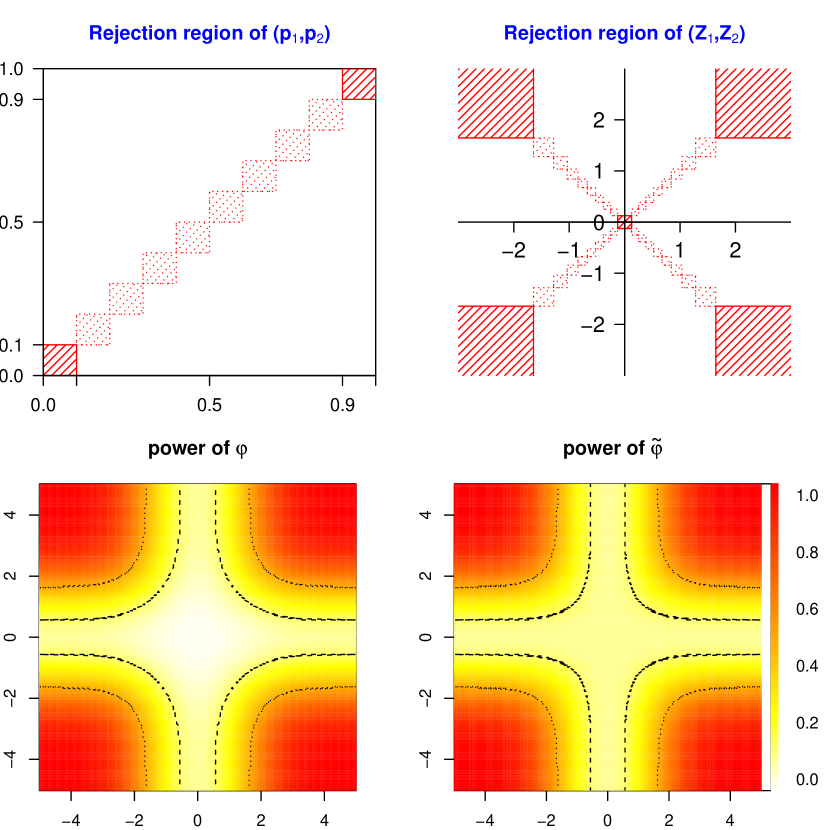
Figure 1: The top two plots: rejection regions of $\varphi^{\prime}$ and $\widetilde{\varphi}$ in the p-value space and the test statistic space, using $\alpha=0.2$. The sold shaded region is the rejection region of $\varphi^{\prime}$, while the rejection region of $\widetilde{\varphi}$ also includes in the dotted shaded squares. The Bottom two plots: power comparison of $\varphi$ and $\widetilde{\varphi}$. The dashed line is where power is at $0.15$ and the dotted line is where the power is $0.5$.

The more powerful test $\varphi^{\prime}$ increases power by strangely rejecting $H^{2/2}_{0}$ when both input p-values are large enough. We now use this same approach to show that without the monotonicity constraint, any GBHPC p-value is inadmissible for any $n$ and any $r\in 2{:}n$. The counter-examples reject $H^{r/n}_{0}$ when all p-values are large. The idea is to show that for any GBHPC test, it’s always possible to add a “box”-shaped rejection region like the square around the origin in the right panel of Figure 1 while still keeping the test valid. The point is not to advocate for such tests, but rather to reinforce the idea that admissibility is only a useful concept within a well chosen class of functions.

We need the following mild technical constraint to guarantee that the “box” we choose can really increase power at least in one alternative hypothesis.

Assumption 4.

For each $i\in 1{:}n$, there exists $\theta_{i}^{0}\in\Theta_{0i}$ that $\mathbb{P}_{\theta_{i}^{0}}(P_{i}\leq\alpha)=\sup_{\theta_{i}\in\Theta_{0i}}(P_{i}\leq\alpha)$ for $\forall\alpha\in[0,1]$. Let $\theta^{0}=(\theta_{1}^{0},\theta_{2}^{0},\cdots,\theta_{n}^{0})$. Then for any set $A$, if $\mathbb{P}_{\theta^{0}}(A)>0$, then there exists $\theta^{1}\in\Theta_{1}^{r/n}$ that $\mathbb{P}_{\theta^{1}}(A)>0$.

Theorem 3.6.

Let $P_{1},\dots,P_{n}$ be independent p-values satisfying assumptions 1, 2 and 4. Let $1<r\leq n$ and $\alpha\in(0,1)$. Then any monotone $\alpha$-admissible combined p-value for testing $H^{r/n}_{0}$ is not $\alpha$-admissible without the monotonicity constraint.

Proof.

Using 3.3, we only need to consider a GBHPC p-value $f^{\star}$ which is defined in 6. Let $\theta^{0}=(\theta_{1}^{0},\theta_{2}^{0},\cdots,\theta_{n}^{0})$ be the parameter in Assumption 4. define

$$R=\{\bm{p}\in[0,1]^{n}:f^{\star}(\bm{p})\leq\alpha\}=\bigcap_{u\subset 1{:}n\atop|u|=n-r+1}R_{u}$$

where $R_{u}=\{\bm{p}\in[0,1]^{n}:g_{u}(\bm{p}_{u})\leq\alpha\}$ and $g_{u}$ is defined in (2).

First, as $\mathbb{P}_{\theta^{0}}(f^{\star}\leq\alpha)\leq\alpha<1$ and $f^{\star}$ is non-decreasing, there exists some $p_{0}<1$ such that if $p_{j}\geq p_{0}$ for all $j\in 1{:}n$ then $f^{\star}(\bm{p})>\alpha$.

Then, we show that there must exist a set $u^{\star}$ with $\mathbb{P}_{\theta^{0}}(R_{u^{\star}}\cap R^{c})=\epsilon>0$, where $R^{c}$ is the complement set of $R$. If this doesn’t hold, then it means that for any $u\subset 1{:}n$ with $|u|=n-r+1$, the equation $1_{f^{\star}(\bm{p})\leq\alpha}(\bm{p})=1_{g_{u}(\bm{p}_{u})\leq\alpha}(\bm{p})\leavevmode\nobreak\ a.e.\leavevmode\nobreak\ \mathbb{P}_{\theta^{0}}$ holds. This implies that $1_{f^{\star}\leq\alpha}$ doesn’t depend on $\bm{p}_{-u}$ except for a zero probability set under $\mathbb{P}_{\theta^{0}}$. As $\cup_{u\subset 1{:}n\atop|u|=n-r+1}{-}u=1{:}n$, we get that $1_{f^{\star}\leq\alpha}$ doesn’t depend on any $p_{j}$ except for a zero probability set under $\mathbb{P}_{\theta^{0}}$, which implies that $1_{f^{\star}\leq\alpha}\equiv 1$ or $0\leavevmode\nobreak\ a.e.\leavevmode\nobreak\ \mathbb{P}_{\theta^{0}}$. It’s obvious that such a test is either invalid or trivially not admissible, which contradicts our assumptions.

As a consequence, we have $\mathbb{P}_{\theta^{0}}(f^{\star}\leq\alpha)=\mathbb{P}_{\theta_{0}}(R_{u^{\star}})-\epsilon\leq\alpha-\epsilon$. Notice that $\mathbb{P}_{\theta^{0}}(f^{\star}\leq\alpha)=\mathbb{E}_{\theta^{0}_{-u}}\big{(}\mathbb{P}_{\theta^{0}_{u}}[f^{\star}\leq\alpha\mid\bm{P}_{-u}]\big{)}$ for any $u$. using the fact that $f^{\star}$ is non-decreasing, $\mathbb{P}_{\theta^{0}_{u}}[f^{\star}\leq\alpha\mid\bm{P}_{-u}=\bm{p}_{-u}]$ is non-increasing in $\bm{p}_{-u}$. Thus there exists $\widetilde{p}<1$, such that for any $u$, if $\bm{p}_{-u}\in[\widetilde{p},1]^{r-1}$, then

$$\mathbb{P}_{\theta^{0}_{u}}[f^{\star}\leq\alpha\mid\bm{P}_{-u}=\bm{p}_{-u}]\leq\alpha-\epsilon.$$

Let $p^{\star}=\max(p_{0},\widetilde{p},1-\epsilon^{1/(n-r+1)})$ and $S=\cap_{i}\{\bm{p}\in[0,1]^{n}:p_{i}\geq p^{\star}\}$. Then we construct a new test with critical function $\varphi$: $\varphi=\mathbbm{1}_{f^{\star}\leq\alpha}+\mathbbm{1}_{S}$.

As $\{\bm{p}\in[0,1]^{n}:f^{\star}(\bm{p})\leq\alpha\}\cap S=\varnothing$, we know that $\varphi$ is at least as powerful as $\mathbbm{1}_{f^{\star}\leq\alpha}$. Using Assumption 4, as $\mathbb{P}_{\theta^{0}}(S)\geq(1-p^{\star})^{n}>0$, there exists $\theta^{1}\in\Theta_{1}^{r/n}$ with $\mathbb{P}_{\theta^{1}}(S)>0$. Thus, $\varphi$ strictly dominates $\mathbbm{1}_{f^{\star}\leq\alpha}$ at $\theta^{1}$. Finally, for $\forall\bm{p}\in[0,1]^{n}$ and $\forall u\subset 1{:}n$ with $|u|=n-r+1$, if $\theta_{u}\in H^{1/{n-r+1}}$, then

$$\mathbbm{E}_{\theta_{u}}[\varphi\mid\bm{P}_{-u}=\bm{p}_{-u}] \leq\mathbb{P}_{\theta_{u}}[f^{\star}\leq\alpha\mid\bm{P}_{-u}=\bm{p}_{-u}]+\epsilon\mathbbm{1}_{\bm{p}_{-u}\in[p^{\star},1]^{r-1}}$$

$$\leq\mathbb{P}_{\theta_{u}^{0}}[f^{\star}\leq\alpha\mid\bm{P}_{-u}=\bm{p}_{-u}]+\epsilon\mathbbm{1}_{\bm{p}_{-u}\in[p^{\star},1]^{r-1}}\leq\alpha.$$

The second inequality above follows from Assumption 4, independence of the individual p-values and monotonicity of $f^{\star}$. Thus $\varphi$ is still an $\alpha$-level test for $H^{r/n}$. This shows that $f^{\star}$ is not $\alpha$-admissible. ∎

4 Simulation

In this simulation example, we compare the power of several GBHPC p-values testing for the PC hypothesis $H_{0}^{r/n}$ with $n=8$ studies and $r=2$. Compared with other $r$ values, the null hypothesis $H_{0}^{2/n}$ is often of particular interest as it tests whether the significance of the effect can replicate or not across studies. It is also the case where the computational cost of non-symmetric GBHPC p-value would typically not be a concern.

We consider the alternative whose true number of non-null hypotheses is one of $r_{0}=2,4,6$. We assume that all the individual hypotheses are independent. Each p-value $P_{i}$ is a two-sided p-value of the corresponding z-value $Z_{i}\sim\mathcal{N}(\sqrt{N_{i}}\mu_{i},1)$ for $i=1,2,\dots,8$. We set three of the sample sizes $N_{i}$ of the eight individual studies to $100$, another three of them to $500$ and the last two to $1000$. for the effects $\mu_{i}$, if $H_{0i}$ is true, then $\mu_{i}=0$. Otherwise when $H_{0i}$ is false, we generate $\mu_{i}\overset{i.i.d}{\sim}\text{Gamma}(\alpha_{0},\beta_{0})$. We define $\mu_{0}=\alpha_{0}/\beta_{0}$ and $\sigma_{0}=\sqrt{\alpha_{0}/\beta_{0}^{2}}$ which are the mean and standard deviation of the non-null effect across studies. We compare the power of each GBHPC p-value as a function of $(\mu_{0},\sigma_{0})$ at the significance level of $\alpha=0.05$.

We compare three GBHPC P-values, whose meta-analysis P-values $g_{u}$ are from examples 1, 2 and 3 respectively. The results are shown in Figure 2. For each $r_{0}$ and each form of the GBHPC p-value, we plot a power map against $(\mu_{0},\sigma_{0})$. To better illustrate the difference across methods, for Simes and weighted Stouffer GBHPC p-values, we plot their powers after they are substracted by the powers of Fisher’s BHPC p-value at the corresponding location. Here are some observations from the simulation results. First, Figure 2 shows that when $r_{0}=2$, Simes BHPC p-value is the most powerful in a large region of the alternative space. The reason is that, for each subset of hypotheses with size $n-r+1=n-1$, at the worst case there is only one non-null individual hypothesis, where simes should be most powerful in detecting extreme p-values. Second, the Weighted Stouffer GBHPC p-value can have higher power than Fisher’s BHPC p-value when $r_{0}>r=2$ and when the effect heterogeneity across non-null studies ($\sigma_{0}$) is not too large to dominate the average effect ($\mu_{0}$). Notice that we are using two-sided p-values to make a fair comparison of the methods, thus taking $\sqrt{n_{i}}$ as weights in Stouffer’s method would not be optimal. However, as we have discussed in Example 3 and shown here, it can still provide a good test with two-sided p-value. If individual p-values were one-sided, then we would have seen a even higher power gain. Finally, the three methods would not have a noticeable difference in power when the power is too low or too high. Most of the difference apprear when the power is in the range of $0.4$ to $0.6$.

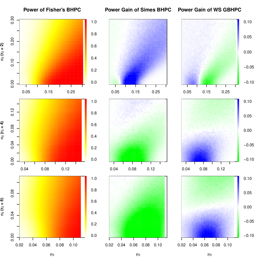
Figure 2: Power comparison of GBHPC p-values: Each row is for one $r_{0}$ value and each column is for one form of GBHPC p-value. the significance level is $\alpha=0.05$. The first column are power maps Fisher’s BHPC p-value against $(\mu_{0},\sigma_{0})$. the last two columns are the power difference of Simes and Weighted Stouffer’s GBHPC p-values against Fisher’s p-value. The green color indicates a power loss compared with Fisher’s BHPC p-value while the blue color shows a power gain.

5 Real data analysis

Compared with BHPC p-values, GBHPC p-values has the flexiblility to make use of the possibly complex dependency structure across studies, thus may achieve higher power. We use a real data example to illustrate this benefit.

The dataset (Ruff et al., 2014) is a pooled dataset from four randomized clinical trials aiming to measure the relative benefit of new anticoagulants (NOAC) compared with an old drug called warfarin for stroke prevention. One primary goal in the original paper was to assess and compare the efficiency of these new drugs in different clinical subgroups of patients. The subgroups and the data are shown in Table 2(a). The data ($m/N$) records that among $N$ samples the number of samples who suffer a stroke or systemic embolic event is $m$. Thus, to test the different between using the old and new drug, we estimate the odds ratio and compute p-values for each subgroup using Fisher’s exact test.

We can use PC tests to assess the consistency of the drug efficiency across different subgroups, which is one of the major interest of the original paper. One major difficulty for applying PC tests (and meta-analysis) to theses subgroups is that these subgroups are correlated. For example, the subgroup of age $\leq 75$ clearly overlaps with the subgroup of female. When there is unknown dependency across individual hypotheses, the only BHPC p-values available are to have the meta-analysis p-value $g$ be either the Bonferroni or Simes p-value. The left column of Table 2(b) are the values of the Bonferroni BHPC p-values $p_{r/n}^{\text{Bon}}$ for $H_{0}^{r/n}$ with $n=18$ and $r$ changing from $2$ to $18$. As $p_{r/n}^{\text{Bon}}$ is increasing in $r$ except when $r$ change from $16$ to $17$, the values of Simes BHPC p-values will agree with $p_{r/n}^{\text{Bon}}$ except when $r=16$.

The question is: is it possible to get smaller valid p-values? The answer is YES, by using a non-symmetric GBHPC p-value. Notice that the groups which represent different levels of the same grouping factor do not share samples, thus have independent p-values. For example, the three p-values for the three $\text{CHADS}_{2}$ groups are independent. Let $1{:}18=\cup_{i=1}^{8}I_{i}$ where each $I_{i}$ is the index set of subgroups using the $i$th grouping factor. Then, to build a GBHPC p-value $p_{r/n}^{\text{new}}$, we construct $g_{u}(p_{u})$ for each $u\in 1{:}n$ with $|u|=n-r+1$ as follows: for each $I_{i}\cap u\neq\varnothing$, a Fisher’s p-value (Example 2) $p_{u,i}$ is calculated on $p_{u\cap I_{i}}$, then

$$g_{u}(p_{u})=\big{|}\{i:u\cap I_{i}\neq\varnothing\}\big{|}\cdot\left(\min_{i}p_{u,i}\right)$$

which is a Bonferroni combination of p-values across the grouping factors. The above construction obviously provides a valid GBHPC p-value.

The next concern is the computation of $p_{r/n}^{\text{new}}$. We claim that for any given $r$, it can be quickly computed by checking Table 2(c). Table 2(c) are all $p_{u,i}$ values that can possibly affect the value of $p_{r/n}^{\text{new}}$ for any $r$. Notice that

$$f^{\star}(p)=\max_{u,|u|=n-r+1}\min_{i}p_{u,i}.$$

Since $p_{u,i}$ is symmetric, it can possibly influence $f^{\star}$ only when $p_{u,i}$ is the Fisher’s combination on the largest $|\mu\cap I_{i}|$ p-values in $I_{i}$. This explains the values in Table 2(c). Then, computing $p_{r/n}^{\text{new}}$ becomes easy. One nice phenomenon of the p-values in Table 2(c) is that p-values on the first row are uniformly smaller than the p-values on the second row, the latter further uniformly smaller than p-values on the third row. Such a property can greatly simplify the computation. The calculation of $g_{u}(p_{u})$ is by replacing some $p_{I_{i},i}$ (first row p-value in Table 2(c)) with some larger $p_{u,i}$ (higher row p-values) or completely removing it. For example when $r=4$, there are $n-r+1=3$ indices that are not in $u$. Thus for any $u$, at most $3$ of the $p_{I_{i},i}$ can be replaced. If we denote $p_{I_{(1)},(1)}\leq\dots p_{I_{(8)},(8)}$, then it’s easy to see that $p_{4/n}^{\text{new}}=8p_{I_{(4)},(4)}$.

It is a bit more complicated when $r\geq 9$. First, notice that for the $r-1$ indices that are not in $\mathrm{argmax}_{u}g_{u}(p_{u})$, we should have each $I_{i}\cap-u\neq\varnothing$ to avoid appearance of p-values on the first row in Table 2(c). Then the problem becomes optimizing the location of the rest $r-1-8$ indices to maximize $g_{u}(p_{u})$. For example when $r=12$, there are $4$ indices left and we now just need to examine the p-values on the second and third row in Table 2(c). If we denote the p-values on the second row as $p_{u_{i},i}$ and define $p_{u_{(1)},(1)}\leq\dots p_{u_{(8)},(8)}$, using a similar argument as $r=4$, one can check that $p_{12/n}^{\text{new}}=\max\{7p_{u_{(2)},(2)},6p_{u_{(3)},(3)},5p_{u_{(4)},(4)}\}$.

Finally, the $p_{r/n}^{\text{new}}$ values for all $r=2,\dots,18$ are shown in Table 2(b). Compared with Bonferroni BHPC p-values, the new GBHPC p-values can be much smaller especially when $r$ is small. Both methods give a $95\%$ confidence interval of the true proportion of non-null hypotheses $r_{0}/n$ as $r_{0}/n\in[0.72,1]$.

(a)

	Pooled NOAC (events)	Pooled Warfarin (events)	Estimated Odds Ratio	p value
Age(years)
$\leq 75$	496/18073	578/18004	0.85	9.26E-03
$\geq 75$	415/11188	532/11095	0.76	6.61E-05
Sex
Female	382/10941	478/10839	0.78	5.00E-04
Male	531/18371	634/18390	0.83	2.38E-03
Diabetes
No	622/20216	755/20238	0.82	2.93E-04
Yes	287/9096	356/8990	0.79	3.81E-03
Previous stroke or TIA
No	483/20699	615/20637	0.78	4.65E-05
Yes	428/8663	495/8635	0.85	2.14E-02
Creatinine clearance (mL/min)
$\leq 50$	249/5539	311/5503	0.79	6.24E-03
$50-80$	405/13055	546/13155	0.74	5.85E-06
$\geq 80$	256/10626	255/10533	1.00	9.64E-01
$\text{CHADS}_{2}$ score
$0-1$	69/5058	90/4942	0.75	7.83E-02
$2$	247/9563	290/9757	0.87	1.05E-01
$3-6$	596/14690	733/14528	0.80	5.21E-05
VKA status
Naive	386/13789	513/13834	0.75	2.19E-05
Experienced	522/15514	597/15395	0.86	1.61E-02
Centre-based TTR
$\leq 66$	509/16219	653/16297	0.78	2.49E-05
$\geq 66$	313/12742	392/12904	0.80	4.68E-03

(b)

r	$p_{r/n}^{\text{Bon}}$	$p_{r/n}^{\text{new}}$
2	3.73E-04	4.49E-05
3	3.98E-04	4.66E-05
4	6.98E-04	7.50E-05
5	7.29E-04	1.18E-04
6	8.59E-04	1.31E-04
7	3.52E-03	1.39E-04
8	5.50E-03	4.23E-04
9	2.38E-02	1.90E-02
10	3.43E-02	2.66E-02
11	3.75E-02	2.81E-02
12	4.37E-02	4.63E-02
13	5.56E-02	6.45E-02
14	8.07E-02	6.45E-02
15	8.56E-02	7.36E-02
16	2.35E-01	7.36E-02
17	2.11E-01	2.11E-01
18	9.64E-01	9.64E-01

(c)

	Age	Sex	Diabetes	Stroke or TIA	Creatinine	$\text{CHADS}_{2}$	VKA	TTR
$H_{0}^{1/k_{i}}$	9.37E-06	1.74E-05	1.64E-05	1.47E-05	5.83E-06	5.29E-05	5.61E-06	1.98E-06
$H_{0}^{2/k_{i}}$	9.26E-03	2.38E-03	3.81E-03	2.14E-02	3.68E-02	4.78E-02	1.61E-02	4.68E-03
$H_{0}^{3/k_{i}}$	–	–	–	–	9.64E-01	1.05E-01	–	–

Table 2: (a) The original data and individual p-values: the blue color highlights individual p-values that are not significant at level $\alpha=0.05$; (b) the values of Bonferroni BHPC p-value and the new GBHPC p-values when $r$ changes in $H_{0}^{r/n}$; (c) the grouping factor level combined p-values: here $k_{i}=|I_{i}|$ and each p-value is the Fisher’s BHPC p-value on $p_{I_{i}}$ testing for $H_{0}^{r_{1}/k_{i}}$ where $r_{1}=1,2,3$.

6 Conclusion and future work

Partial conjunction hypotheses are natural hypotheses to test for measuring repeated effects across settings/studies. The null is rejected only when at least $r$ hypotheses are non-null. By testing PC hypotheses at different $r$ values, one can also construct a confidence interval of $r_{0}/n$, the true proportion of non-null hypotheses.

This paper characterizes the admissible p-values for a partial conjunction test of independent hypotheses or hypotheses with positively dependent P-values, within the class of non-decreasing p-values. Any monotone admissible p-value for $H_{0}^{r/n}$ is the maximum of the non-decreasing p-values for the global null in each combination of $n-r+1$ hypotheses, which we call GBHPC p-values. We have shown that for sensitive GBHPC p-values, as long as each meta-analysis p-value of the $n-r+1$ hypotheses is admissible, the combined p-value is monotone admissible. A consequence is that among combined p-values that only depend on the order statistics of individual p-values, the original BHPC p-values are the only monotone admissible ones. We also have found inadmissibility of GBHPC p-values without the monotonicity constraint. However, the dominated tests only have a moderate power gain at low power regions in the alternative space. Since these counter-examples are not monotone, they are hard to be explained in practice thus not reasonable choices.

In summary, we illustrated the properties of tests for a PC hypothesis and characterized a class of good tests called GBHPC p-values. Compared with its symmetric form, the BHPC p-values, GBHPC p-values have more flexibility to adapt to complicated problem structure, thus can have power gain at important regions in the alternative space, as we showed in our simulations and real data examples. The computational cost of non-symmetric GBHPC p-values can be of a concern, but there are special cases where GBHPC p-values are computable. One of the future directions is to expand the applications where computable GBHPC p-values are available.

One other direction is to understand properties of the confidence interval of $r$ constructed by GBHPC p-values. In Section 5, the result showed that though the newly proposed GBHPC p-values can be much smaller than Simes or Bonferroni BHPC p-values at many $r$ values, the confidence interval that the two methods constructed are still the same. Finally, there are variations of partial conjunctions that are useful in practice. For example, the count of replicability may vary for different hypotheses. Replication of effects from two distinct classes can be of more interest than replication in two similar classes. Another variation is to require that a null hypothesis is rejected only when there are at least $r$ non-nulls with the same sign of effect. Such hypotheses can have very complex alternative and null space, and it can be the future work to understand their properties.