From the Lorentz Group to the Celestial Sphere

 

Blagoje Oblak^∗

Physique Théorique et Mathématique

Université Libre de Bruxelles and International Solvay Institutes

Campus Plaine C.P. 231, B-1050 Bruxelles, Belgium

Abstract

In these lecture notes we review the isomorphism between the (connected) Lorentz group and the set of conformal transformations of the sphere. More precisely, after establishing the main properties of the Lorentz group, we show that it is isomorphic to the group $\mathrm{SL}(2,\mathbb{C})$ of complex $2\times 2$ matrices with unit determinant. We then classify conformal transformations of the sphere, define the notion of null infinity in Minkowski space-time, and show that the action of Lorentz transformations on the celestial spheres at null infinity is precisely that of conformal transformations. In particular, we discuss the optical phenomena observed by the pilots of the Millenium Falcon during the jump to lightspeed.

This text, aimed at undergraduate students, was written for the seventh Brussels Summer School of Mathematics^† that took place at Université Libre de Bruxelles in August 2014. An abridged version has been published in the proceedings of the school, “Notes de la septième BSSM”, printed in July 2015.

^∗ Research Fellow of the Fund for Scientific Research-FNRS Belgium. E-mail: boblak@ulb.ac.be
^† Website: http://bssm.ulb.ac.be/

Introduction

The Lorentz group is essentially the symmetry group of special relativity. It is commonly defined as a set of (linear) transformations acting on a four-dimensional vector space $\mathbb{R}^{4}$, representing changes of inertial frames in Minkowski space-time. But as we will see below, one can exhibit an isomorphism between the Lorentz group and the group of conformal transformations of the sphere $S^{2}$; the latter is of course two-dimensional. This isomorphism thus relates the action of a group on a four-dimensional space to its action on a two-dimensional manifold. At first sight, such a relation seems surprising: loosely speaking, one expects to have lost some information in going from four to two dimensions. In particular, the isomorphism looks like a coincidence of the group structure: there is no obvious geometric relation between the original four-dimensional space on the one hand, and the sphere on the other hand.

The purpose of these notes is to show that such a relation actually exists, and is even quite natural. Indeed, by defining a notion of “celestial spheres”, one can derive a direct link between four-dimensional Minkowski space and the two-dimensional sphere. In short, the celestial sphere of an inertial observer in Minkowski space is the sphere of all directions towards which the observer can look, and coordinate transformations between inertial observers (i.e. Lorentz transformations) correspond to conformal transformations of this sphere [1, 2, 3, 4]. In this work we will review this construction in a self-contained way.

Keeping this motivation in mind, the text is organized as follows. In section 1, we review the basic principles of special relativity and define the natural symmetry groups that follow, namely the Poincaré group and its homogeneous subgroup, the Lorentz group [5, 6, 7]. This will also be an excuse to discuss certain elegant properties of the Lorentz group that are seldom exposed in elementary courses on special relativity, in particular regarding the physical meaning of the notion of “rapidity” [8, 9, 10]. In section 2, we then establish the isomorphism between the connected Lorentz group and the group $\mathrm{SL}(2,\mathbb{C})$ of complex, two by two matrices of unit determinant, quotiented by its center $\mathbb{Z}_{2}$. We also derive the analogue of this result in three space-time dimensions. Section 3 is devoted to the construction of conformal transformations of the sphere; it is shown, in particular, that such transformations span a group isomorphic to $\mathrm{SL}(2,\mathbb{C})/\mathbb{Z}_{2}$ $-$ a key result in the realm of two-dimensional conformal field theories [11, 12]. At that point, the stage will be set for the final link between the Lorentz group and the sphere, which is established in section 4. The conclusion, section 5, relates these observations to some recent developments in quantum gravity $-$ in particular BMS symmetry [13, 14, 15, 16, 17, 18, 19, 20] and holography [21, 22, 23, 24, 25].

The presentation voluntarily starts with fairly elementary considerations, in order to be accessible (hopefully) to undergraduate students. Though some basic knowledge of group theory and special relativity should come in handy, no prior knowledge of differential geometry, general relativity or conformal field theory is assumed. In particular, sections 1 and 2 are mostly based on the undergraduate-level lecture notes [5].

1 Special relativity and the Lorentz group

In this section, after reviewing the basic principles of special relativity (subsection 1.1), we define the associated symmetry groups (subsection 1.2) and introduce in particular the Lorentz group. In subsection 1.3, we then define certain natural subgroups of the latter. Subsection 1.4 is devoted to the notion of Lorentz boosts and to the associated additive parameter, which turns out to have the physical meaning of “rapidity”. Finally, in subsection 1.5 we show that any Lorentz transformation preserving the orientation of space and the direction of time flow can be written as the product of two rotations and a boost, and then use this result in subsection 1.6 to classify the connected components of the Lorentz group. All these results are well known; the acquainted reader may safely jump directly to section 2. The presentation of this section is mainly inspired from the lecture notes [5] and [6]; more specialized references will be cited in due time.

1.1 The principles of special relativity

1.1.1 Events and reference frames

In special relativity, natural phenomena take place in the arena of space-time. The latter consists of points, called events, which occur at some position in space, at some moment in time. Events are seen by observers who use coordinate systems, also called reference frames, to specify the location of an event in space-time. In the realm of special relativity, reference frames typically consist of three orthonormal spatial coordinates $(x^{1},x^{2},x^{3})$ and one time coordinate $t$, measured by a clock carried by the observer. For practical purposes, the speed of light in the vacuum,

$$c=299\,792\,458\;\text{m/s},$$ (1.1)

is used as a conversion factor to express time as a quantity with dimensions of distance. This is done by defining a new time coordinate $x^{0}\equiv ct$.

Thus, in a given reference frame, an event occurring in space-time is labelled by its four coordinates $(x^{0},x^{1},x^{2},x^{3})$, collectively denoted as $(x^{\mu})$. (From now one, greek indices run over the values $0$, $1$, $2$, $3$.) Of course, the event’s existence is independent of the observers who see it, but its coordinates are not: if Alice and Bob are two observers looking at the same event, Alice may use a set of four numbers $(x^{\mu})$ to describe its location, but Bob will in general use different coordinates $(x^{\prime\mu})$ to locate the same event. Besides, if we do not specify further the relation between Alice and Bob, there is no link whatsoever between the coordinates they use. What we need are restrictions on the possible reference frames used by Alice and Bob; the principles of special relativity will then apply only to those observers whose reference frames satisfy the given restrictions.

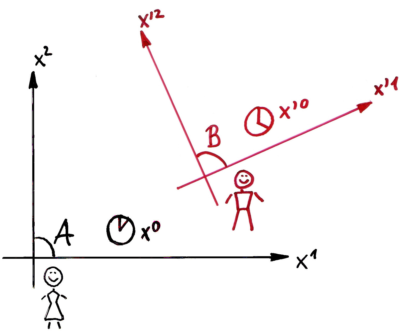
Figure 1: Alice (drawn in black) and Bob (drawn in red) in space-time, with their respective reference frames (including clocks); for simplicity, only two spatial dimensions are represented. Looking at the same event, Alice and Bob will typically associate different coordinates with it. In general, there is no way to relate the coordinates of Alice’s frame to those of Bob’s frame.

1.1.2 The principles of special relativity

We now state the defining assumptions of special relativity. The three first basic assumptions are homogeneity of space-time, isotropy of space and causality [8, 7]. The remaining principles, discussed below, lead to constraints on the relation between reference frames. To expose these principles, we first need to define the notion of inertial frames.

According to the principle of inertia, a body left to itself, without forces acting on it, should move in space in a constant direction, with a constant velocity. Obviously, this principle cannot hold in all reference frames. For example, suppose Alice observes that the principle of inertia is true in her reference frame (for example by throwing tennis balls in space and observing that they move in straight lines at constant velocity). Then, if Bob is accelerated with respect to Alice, he will naturally use a comoving frame and the straight motions seen by Alice will become curved motions in his reference frame. Therefore, if two reference frames are accelerated with respect to each other, the principle of inertia cannot hold in both frames. More generally, we call inertial frame a reference frame in which the principle of inertia holds [7]; the results of special relativity apply only to such frames. Accordingly, an observer using an inertial frame is called an inertial observer; in physical terms, it is an observer falling freely in empty space. We will see in subsection 1.2 what restrictions are imposed on the relation between coordinates of inertial frames; at present, we already know that, if two such frames move with respect to each other, then this motion must take place along a straight line, at constant velocity.

Given this definition, we are in position to state the two crucial defining principles of special relativity. The first, giving its name to the theory, is the principle of relativity (in the restricted sense [26]), which states that the laws of Nature must take the same form in all inertial frames. In other words, according to this principle, there exists no privileged inertial frame in the Universe: there is no experiment that would allow an experimenter to distinguish a given inertial frame from the others. This is a principle of special relativity in that it only applies to inertial frames; a principle of general relativity would apply to all possible reference frames, inertial or not. The latter principle leads to the theory of general relativity, which we will not discuss further here.

The second principle is Einstein’s historical “second postulate”, which states that the speed of light in the vacuum takes the same value $c$, written in (1.1), in all inertial frames. In fact, if one assumes that Maxwell’s theory of electromagnetism holds, then the second postulate is a consequence of the principle of relativity. Indeed, saying that the speed of light (in the vacuum) is the same in all inertial frames is really saying that the laws of electromagnetism are identical in all inertial frames [7].

1.2 The Poincaré group and the Lorentz group

We now work out the relation between coordinates of inertial frames; the set of all such relations will form a group, called the Poincaré group. We will see that the second postulate is crucial in determining the form of this group, through the notion of “space-time interval”.

1.2.1 Linear structure

Suppose $A$ and $B$ are two inertial frames, i.e. the principle of inertia holds in both of them. Then, a particle moving along a straight line at constant velocity, as seen from $A$, must also move at constant velocity along a straight line when seen from $B$. Thus, calling $(x^{\mu})$ the space-time coordinates of $A$ and $(x^{\prime\mu})$ those of $B$, the relation between these coordinates must be such that any straight line in the coordinates $x^{\mu}$ is mapped on a straight line in the coordinates $x^{\prime\mu}$. The most general transformation satisfying this property is a projective map [6], for which

$$x^{\prime\mu}=\frac{a^{\mu}+{\Lambda^{\mu}}_{\nu}x^{\nu}}{b+c_{\mu}x^{\mu}}\quad\forall\,\mu=0,1,2,3.$$ (1.2)

(From now on, summation over repeated indices will always be understood.) Here $a^{\mu}$, ${\Lambda^{\mu}}_{\nu}$, $b$ and $c_{\mu}$ are constant coefficients. If we insist that points having finite values of coordinates in $A$ remain with finite coordinates in $B$, we must set $c_{\mu}=0$. Then, absorbing the constant $b$ in the parameters $a^{\mu}$ and ${\Lambda^{\mu}}_{\nu}$, the transformation (1.2) reduces to

$$x^{\prime\mu}={\Lambda^{\mu}}_{\nu}x^{\nu}+a^{\mu}.$$ (1.3)

Thus, the principle of inertia endows space-time with a linear structure. In order for the transformation (1.3) to be invertible, we must also demand that the matrix $\Lambda=({\Lambda^{\mu}}_{\nu})$ be invertible. Apart from that, using only the principle of inertia, we cannot go further at this point. The principle of relativity will set additional restrictions on $\Lambda$.

1.2.2 Invariance of the interval

Let again $A$ be an inertial frame and let ${\cal P}$ and ${\cal Q}$ be two events in space-time. Call $\Delta x^{\mu}$ the components of the vector going from ${\cal P}$ to ${\cal Q}$ in the frame $A$. Then, we call the number

$$\Delta s^{2}\equiv-(\Delta x^{0})^{2}+(\Delta x^{1})^{2}+(\Delta x^{2})^{2}+(\Delta x^{3})^{2}\equiv\eta_{\mu\nu}\Delta x^{\mu}\Delta x^{\nu}$$ (1.4)

the square of the interval between ${\cal P}$ and ${\cal Q}$. The matrix

$$\eta=(\eta_{\mu\nu})=\begin{pmatrix}-1&0&0&0\\ 0&1&0&0\\ 0&0&1&0\\ 0&0&0&1\end{pmatrix}$$ (1.5)

appearing in this definition is called the Minkowski metric matrix. The terminology associated with definition (1.4) may seem inconsistent, in that we call “square of the interval between two events” a quantity that seems to depend not only on the events, but also on the coordinates chosen to locate them (in the present case, the separation $\Delta x^{\mu}$). This is not the case, however, thanks to the following important result:

Proposition.

Let $A$ and $B$ be two inertial frames, ${\cal P}$ and ${\cal Q}$ two events, the square of the interval between them being $\Delta s^{2}$ in the coordinates of $A$ and $\Delta s^{\prime\,2}$ in those of $B$. Then,

$$\Delta s^{2}=\Delta s^{\prime\,2}\quad\text{(``invariance of the interval'').}$$ (1.6)

In other words, the number (1.4) does not depend on the inertial coordinates used to define it.

Proof.

First suppose that ${\cal P}$ and ${\cal Q}$ are light-like separated, i.e. that there exists a light ray going from ${\cal P}$ to ${\cal Q}$ (or from ${\cal Q}$ to ${\cal P}$). Then, $\Delta s^{2}=0$ by construction. But, by Einstein’s second postulate, the speed of light is the same in both reference frames $A$ and $B$, so $\Delta s^{\prime\,2}=0$ as well. Thus,

$$\Delta s^{2}=0\quad\text{iff}\quad\Delta s^{\prime\,2}=0.$$

Now, since $A$ and $B$ are inertial frames, the relation between their coordinates must be of the linear form (1.3); in particular, $\Delta x^{\mu}={\Lambda^{\mu}}_{\nu}\Delta x^{\nu}$. Therefore $\Delta s^{\prime\,2}$ is a polynomial of second order in the components $\Delta x^{\mu}$. But we have just seen that $\Delta s^{2}$ and $\Delta s^{\prime\,2}$ have identical roots; since polynomials having identical roots are necessarily proportional to each other, we know that there exists some number $K$ such that

$$\Delta s^{\prime\,2}=K\Delta s^{2}.$$ (1.7)

This number $K$ depends on the matrix $\Lambda$ appearing in $\Delta x^{\mu}={\Lambda^{\mu}}_{\nu}\Delta x^{\nu}$, which itself depends on the velocity $\vec{v}$ of the frame $B$ with respect to the frame $A$. (This velocity is constant, since accelerated frames cannot be inertial.) But space is isotropic by assumption, so $K$ actually depends only on the modulus $\|\vec{v}\|$ of $\vec{v}$, and not on its direction. In particular, $K(\vec{v})=K(-\vec{v})$. Since the velocity of $A$ with respect to $B$ is $-\vec{v}$, we know that

$$\Delta s^{2}=K\Delta s^{\prime\,2}\stackrel{{\scriptstyle\text{(\ref{ds2K})}}}{{=}}K^{2}\Delta s^{2},$$

implyiing that $K^{2}=1$. Since real transformations cannot change the signature of a quadratic form, $K$ cannot be negative, so $K=1$. ∎

1.2.3 Lorentz transformations

We now know that coordinate transformations between inertial frames must preserve the square of the interval; let us work out the consequences of this statement for the matrix $\Lambda$ in (1.3). To simplify notations, we will see $(x^{\mu})$ and $(a^{\mu})$ as four-component column vectors, so that (1.3) can be written as

$$x^{\prime}=\Lambda\cdot x+a.$$ (1.8)

Similarly, seeing $(\Delta x^{\mu})$ as a vector $\Delta x$, the square of the interval (1.4) becomes $\Delta s^{2}=\Delta x^{t}\cdot\eta\cdot\Delta x$. (The superscript “$t$” denotes transposition.) Then, since $\Delta x^{\prime}=\Lambda\cdot\Delta x$, demanding invariance of the square of the interval under (1.8) amounts to the equality

$$\Delta s^{\prime\,2}=\Delta x^{t}\cdot\left(\Lambda^{t}\eta\Lambda\right)\cdot\Delta x\stackrel{{\scriptstyle!}}{{=}}\Delta x^{t}\cdot\eta\cdot\Delta x=\Delta s^{2},$$

to be satisfied for any $\Delta x$. Because $\eta$ is non-degenerate, this implies that the matrix $\Lambda$ satisfies

$$\Lambda^{t}\eta\Lambda=\eta.$$ (1.9)

Definition.

The Lorentz group (in four dimensions) is

$$\boxed{\mathrm{O}(3,1)\equiv L\equiv\left\{\Lambda\in\mathrm{M}(4,\mathbb{R})|\Lambda^{t}\eta\Lambda=\eta\right\},}$$ (1.10)

where $\mathrm{M}(4,\mathbb{R})$ denotes the set of real $4\times 4$ matrices. More generally, the Lorentz group in $d$ space-time dimensions, $\mathrm{O}(d-1,1)$, is the group of real $d\times d$ matrices $\Lambda$ satisfying property (1.9) for the $d$-dimensional Minkowski metric matrix $\eta=\text{diag}(-1,\underbrace{1,1,...,1}_{d-1\text{ times}})$.

Remark.

This definition is equivalent to saying that the rows and columns of a Lorentz matrix form a Lorentz basis of $\mathbb{R}^{d}$, that is, a basis $\{e_{0},e_{1},e_{2},...,e_{d-1}\}$ of $d$-vectors $e_{\alpha}$ such that $e_{\alpha}^{\mu}\eta_{\mu\nu}e_{\beta}^{\nu}=\eta_{\alpha\beta}$. The Lorentz group in $d$ space-time dimensions is a Lie group of real dimension $d(d-1)/2$. This is analogous to the orthogonal group $\mathrm{O}(d)$, defined as the set of $d\times d$ matrices ${\cal O}$ satisfying ${\cal O}^{t}{\cal O}=\mathbb{I}$, where $\mathbb{I}$ is the identity matrix. In particular, the rows and columns of an orthogonal matrix form an orthonormal basis of $\mathbb{R}^{d}$.

Definition.

The group consisting of inhomogeneous transformations (1.8), where $\Lambda$ belongs to the Lorentz group, is called the Poincaré group or the inhomogeneous Lorentz group. Its abstract structure is that of a semi-direct product $\mathrm{O}(3,1)\ltimes\mathbb{R}^{4}$, where $\mathbb{R}^{4}$ is the group of translations, the group operation being given by

$$(\Lambda,a)\cdot(\Lambda^{\prime},a^{\prime})=\left(\Lambda\cdot\Lambda^{\prime},a+\Lambda\cdot a^{\prime}\right).$$

Of course, this definition is readily generalized to $d$-dimensional space-times upon replacing $\mathrm{O}(3,1)$ by $\mathrm{O}(d-1,1)$ and $\mathbb{R}^{4}$ by $\mathbb{R}^{d}$. We will revisit the definition of the Lorentz and Poincaré groups at the end of subsection 3.1, with the tools of pseudo-Riemannian geometry. Apart from that, in the rest of these notes, we will mostly need only the homogeneous Lorentz group (1.10) and we will not really use the Poincaré group. We stress, though, that the latter is crucial for particle physics and quantum field theory [27, 28].

1.3 Subgroups of the Lorentz group

The defining property (1.9) implies that each matrix $\Lambda$ in the Lorentz group satisfies $\det(\Lambda)=\pm 1$. This splits the Lorentz group in two disconnected subsets, corresponding to matrices with determinant $+1$ or $-1$. In particular, Lorentz matrices with determinant $+1$ span a subgroup of the Lorentz group $\mathrm{O}(3,1)=L$, called the proper Lorentz group and denoted $\mathrm{SO}(3,1)$ or $L_{+}$. It is the set of Lorentz transformations that preserve the orientation of space.

Another natural subgroup of $L$ can be isolated using (1.9), though in a somewhat less obvious way. Namely, consider the $0-0$ component of eq. (1.9),

$${\Lambda^{\mu}}_{0}\eta_{\mu\nu}{\Lambda^{\nu}}_{0}=-\left({\Lambda^{0}}_{0}\right)^{2}+{\Lambda^{i}}_{0}{\Lambda^{i}}_{0}\stackrel{{\scriptstyle!}}{{=}}\eta_{00}=-1.$$

This implies the property

$$\left({\Lambda^{0}}_{0}\right)^{2}=1+{\Lambda^{i}}_{0}{\Lambda^{i}}_{0}\geq 1,$$ (1.11)

valid for any matrix $\Lambda$ in the Lorentz group. The inequality is saturated only if ${\Lambda^{i}}_{0}=0$ for all $i=1,2,3$. Since the inverse of relation (1.9) implies $\Lambda\eta\Lambda^{t}=\eta$ for any Lorentz matrix $\Lambda$, we also find

$$\left({\Lambda^{0}}_{0}\right)^{2}=1+{\Lambda^{0}}_{i}{\Lambda^{0}}_{i}\geq 1,$$ (1.12)

with equality iff ${\Lambda^{0}}_{i}=0$ for all $i=1,2,3$. Thus, in particular, $|{\Lambda^{0}}_{0}|=1$ iff ${\Lambda^{0}}_{i}={\Lambda^{i}}_{0}=0$ for all $i$, in which case the spatial components ${\Lambda^{i}}_{j}$ of $\Lambda$ form a matrix in $\mathrm{O}(3)$. Just as the determinant property $\det(\Lambda)=\pm 1$, the inequality in (1.11) splits the Lorentz group in two disconnected components, corresponding to matrices with positive or negative ${\Lambda^{0}}_{0}$. Note that the product of two matrices $\Lambda$, $\Lambda^{\prime}$, with positive ${\Lambda^{0}}_{0}$ and ${\Lambda^{\prime\,0}}_{0}$, is itself a matrix with positive $0-0$ component:

$${\left(\Lambda\cdot\Lambda^{\prime}\right)^{0}}_{0} = {\Lambda^{0}}_{\mu}{\Lambda^{\prime\,\mu}}_{0}={\Lambda^{0}}_{0}{\Lambda^{\prime\,0}}_{0}+{\Lambda^{0}}_{i}{\Lambda^{\prime\,i}}_{0}$$ (1.13)

$$\geq {\Lambda^{0}}_{0}{\Lambda^{\prime\,0}}_{0}-\left|{\Lambda^{0}}_{i}{\Lambda^{\prime\,i}}_{0}\right|$$

$$\stackrel{{\scriptstyle\text{(\ref{ineq}),(\ref{ineqBis})}}}{{>}} \sqrt{{\Lambda^{0}}_{i}{\Lambda^{0}}_{i}}\sqrt{{\Lambda^{\prime\,i}}_{0}{\Lambda^{\prime\,i}}_{0}}-\left|{\Lambda^{0}}_{i}{\Lambda^{\prime\,i}}_{0}\right|\geq 0.$$

(In the very last inequality we applied the Cauchy-Schwarz lemma to the spatial vectors whose components are ${\Lambda^{0}}_{i}$ and ${\Lambda^{\prime\,i}}_{0}$.) Therefore, the set of Lorentz matrices $\Lambda$ with positive ${\Lambda^{0}}_{0}$ forms a subgroup of the Lorentz group, called the orthochronous Lorentz group and denoted $\mathrm{O}(3,1)^{\uparrow}$ or $L^{\uparrow}$. As the name indicates, elements of $L^{\uparrow}$ are Lorentz transformations that preserve the direction of the arrow of time.

Given these subgroups, one defines the proper, orthochronous Lorentz group

$$\mathrm{SO}(3,1)^{\uparrow}=L_{+}^{\uparrow}\equiv L_{+}\cap L^{\uparrow},$$

which is of course a subgroup of $L$. In fact, we will see at the end of this subsection that this is the maximal connected subgroup of the Lorentz group. The rows and columns of Lorentz matrices belonging to $L_{+}^{\uparrow}$ form Lorentz bases with a future-directed time-like unit vector, and with positive orientation. The group of orientation-preserving rotations of space, $\mathrm{SO}(3)$, is a natural subgroup of $L_{+}^{\uparrow}$, consisting of matrices of the form

$$\begin{pmatrix}1&0\\ 0&R\end{pmatrix},\quad\text{with }R\in\mathrm{SO}(3).$$ (1.14)

Note that $L_{+}$ can be generated by adding to $L_{+}^{\uparrow}$ the time-reversal matrix

$$T=\begin{pmatrix}-1&0&0&0\\ 0&1&0&0\\ 0&0&1&0\\ 0&0&0&1\end{pmatrix}.$$ (1.15)

Similarly, $L^{\uparrow}$ can be obtained by adding to $L_{+}^{\uparrow}$ the parity matrix

$$P=\begin{pmatrix}1&0&0&0\\ 0&-1&0&0\\ 0&0&-1&0\\ 0&0&0&-1\end{pmatrix}.$$ (1.16)

More generally, the whole Lorentz group $L$ can be obtained by adding $T$ and $P$ to $L_{+}^{\uparrow}$. (Note that $T$ and $P$ do not commute with all matrices in $L_{+}^{\uparrow}$. This should be contrasted with the case of $\mathrm{O}(3)$ and $\mathrm{SO}(3)$, where the three-dimensional parity operator belongs to the center of $\mathrm{O}(3)$.)

1.4 Boosts and rapidity

We have just seen that any rotation, acting only on the space coordinates, is a Lorentz transformation. In the language of inertial frames, this is obvious: if the spatial axes of a frame $B$ are rotated with respect to those of an inertial frame $A$ (and provided the time coordinates in $A$ and $B$ coincide), then $B$ is certainly an inertial frame. The same would be true even in Galilean relativity [7]. In order to see effects specific to Einsteinian special relativity, we need to consider Lorentz transformations involving inertial frames in relative motion.

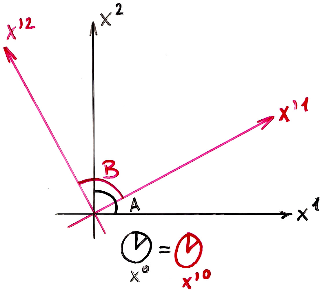
Figure 2: Two inertial frames $A$ and $B$ related by a rotation of their spatial axes (the third space direction is omitted). The clocks of $A$ and $B$ are synchronized.

1.4.1 Boosts

Call $A$ and $B$ the inertial frames used by Alice and Bob, with respective coordinates $(x^{\mu})$ and $(x^{\prime\,\mu})$. Suppose Bob moves with respect to Alice in a straight line, at constant velocity $v$. Without loss of generality, we may assume that the origins of the frames $A$ and $B$ coincide. (If they don’t, just apply a suitable space-time translation to bring them together.) By rotating the spatial axes of $A$ and $B$, we can also choose their coordinates to satisfy $x^{2}=x^{\prime 2}$ and $x^{3}=x^{\prime 3}$. Then, the only coordinates of $A$ and $B$ that are related by a non-trivial transformation are $(x^{0},x^{1})$ and $(x^{\prime 0},x^{\prime 1})$. Finally, using parity and time-reversal if necessary, we may choose the same orientation for the spatial frames of $A$ and $B$, and the same orientation for their time arrows.

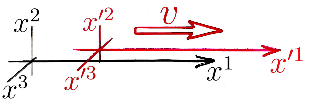
Figure 3: The frame $B$ (in red) is boosted with respect to $A$ (in black) with velocity $v$ along the $x^{1}$ axis. The coordinates $x^{2}$ and $x^{3}$ coincide with $x^{\prime 2}$ and $x^{\prime 3}$. In principle, the clocks of $A$ and $B$ (not represented in this figure) need not tick at the same rate.

Under these assumptions the relation between the coordinates of $A$ and those of $B$ takes the form

$$x^{\prime\mu}={\Lambda^{\mu}}_{\nu}x^{\nu}\quad\text{with}\quad\left({\Lambda^{\mu}}_{\nu}\right)=\begin{pmatrix}p&q&0&0\\ r&s&0&0\\ 0&0&1&0\\ 0&0&0&1\end{pmatrix},$$

where $p$, $q$, $r$ and $s$ are some real coefficients such that $\Lambda$ belongs to $L_{+}^{\uparrow}$ $-$ in particular, $p>0$. Since $B$ moves with respect to $A$ at constant velocity $v$ (along the $x^{1}$ direction), the coordinate $x^{\prime 1}$ of $B$ must vanish when $x^{1}=vt=vx^{0}/c$. By virtue of linearity, we may write

$$x^{\prime 1}=\gamma(v)\cdot\left(x^{1}-\frac{v}{c}x^{0}\right),$$

where $\gamma(v)$ is some $v$-dependent, positive coefficient (on account of the fact that the directions $x^{1}$ and $x^{\prime 1}$ coincide). Demanding that $\Lambda$ satisfies relation (1.9), with the restrictions $p>0$ and $\gamma(v)>0$, then yields

$$\Lambda=\begin{pmatrix}\gamma(v)&-\gamma(v)\cdot v/c&0&0\\ -\gamma(v)\cdot v/c&\gamma(v)&0&0\\ 0&0&1&0\\ 0&0&0&1\end{pmatrix},\quad\text{and}\quad\gamma(v)=\frac{1}{\sqrt{1-v^{2}/c^{2}}}.$$ (1.17)

A Lorentz transformations of this form is called a boost (with velocity $v$ in the direction $x^{1}$). In particular, reality of $\Lambda$ requires $|v|$ to be smaller than $c$: boosts faster than light are forbidden.

Boosts give rise to the counterintuitive phenomena of time dilation and length contraction. Let us briefly describe the former. Suppose Bob, moving at velocity $v$ with respect to Alice, carries a clock and measures a time interval $\Delta t^{\prime}$ in his reference frame; for definiteness, suppose he measures the time elapsed between two consecutive “ticks” of his clock, and let the clock be located at the origin of his reference frame. Call ${\cal P}$ the event “Bob’s clock ticks for the first time at his location at that moment”, and call ${\cal Q}$ the event “Bob’s clock ticks for the second time (at his location at that time)”. Then, in Alice’s coordinates, the time interval $\Delta t$ separating the events ${\cal P}$ and ${\cal Q}$ is not equal to $\Delta t^{\prime}$; rather, according to (1.17), one has $\Delta t=\gamma(v)\Delta t^{\prime}$. Since $\gamma(v)$ is always larger than one, this means that Alice measures a longer duration than Bob: Bob’s time is “dilated” compared to Alice’s time, and $\gamma(v)$ is precisely the dilation factor. This phenomenon is responsible, for instance, for the fact that cosmic muons falling into Earth’s atmosphere can be detected at the level of the oceans even though their time of flight (as measured by an observer standing still on Earth’s surface) is about a hundred times longer than their proper lifetime. In subsection 4.3, we will see that boosts also lead to surprising optical effects on the celestial sphere.

1.4.2 Notion of rapidity

Although the notion of velocity used above is the most intuitive one, it is not the most practical one from a mathematical viewpoint. In particular, composing two boosts with velocities $v$ and $w$ (in the same direction) does not yield a boost with velocity $v+w$. It would be convenient to find an alternative parameter to specify boosts, one that would be additive when two boosts are combined. This leads to the notion of rapidity [9, 5],

$$\chi(v)\equiv\text{argtanh}(v/c),$$ (1.18)

in terms of which the boost matrix (1.17) becomes

$$\Lambda=\begin{pmatrix}\cosh\chi&-\sinh\chi&0&0\\ -\sinh\chi&\cosh\chi&0&0\\ 0&0&1&0\\ 0&0&0&1\end{pmatrix}\equiv L(\chi).$$ (1.19)

One verifies that the composition of two such boosts with rapidities $\chi_{1}$ and $\chi_{2}$ is a boost of the same form, with rapidity $\chi_{1}+\chi_{2}$.

Rapidity is thus the additive parameter specifying Lorentz boosts. It exhibits the fact that boosts along a given axis form a non-compact, one-parameter subgroup of $L_{+}^{\uparrow}$. It also readily provides a formula for the addition of velocities: the composition of two boosts with velocities $v$ and $w$ is a boost with rapidity $\chi(v)+\chi(w)$; equivalently, according to (1.18), the velocity $V$ of the resulting boost is

$$V=c\cdot\tanh(\chi(v)+\chi(w))=c\cdot\tanh\left(\text{argtanh}(v/c)+\text{argtanh}(w/c)\right)=\frac{v+w}{1+vw/c^{2}}.$$

This is the usual formula for the addition of velocities (in the same direction) in special relativity [7].

As practical as rapidity is, its physical meaning is a bit obscure: the definition (1.18) does not seem related to any measurable quantity whatsoever. But in fact, there exist at least three different natural definitions of the notion of “speed”, and rapidity is one of them [10]. To illustrate these definitions, consider an observer, Bob, who travels by train from Brussels to Paris [29], and measures his speed during the journey. For simplicity, we will assume that the motion takes place along the $x$ axis of Alice, an inertial observer standing still on the ground.

A first notion of speed he might want to define is an “extrinsic” one: he lets Alice measure the distance between Brussels and Paris, and the two clocks of the Brussels and Paris train stations are synchronized. Then, looking at the clocks upon departure and upon arrival, he defines his velocity as the ratio of the distance measured by Alice to the duration of his trip, measured by the clocks in Brussels and Paris. The infinitesimal version of velocity is the usual expression $v=dx/dt$, where $x$ and $t$ are the space and time coordinates of an inertial frame which, in general, is not related to Bob. (In the present case, these are the coordinates that Alice, or any inertial observer standing still on the ground, would likely use.)

A second natural definition of speed is given by proper velocity. To define this notion, Bob still lets Alice measure the distance between Brussels and Paris, but now he divides this distance by the duration that he himself has measured using his wristwatch. The infinitesimal version of (the $x$ component of) proper velocity is $u=dx/d\tau$, where $\tau$ denotes Bob’s proper time, defined by

$$d\tau^{2}=dt^{2}-\frac{1}{c^{2}}dx^{2}$$ (1.20)

along Bob’s trajectory. (In (1.20), it is understood that Bob’s trajectory is written as $(t,x(t))$ in the coordinates $(t,x)$ of Alice, but the value of $d\tau$ would be the same in any inertial frame with the same direction for the arrow of time, by virtue of Lorentz-invariance of the interval, eq. (1.6).) If Bob’s motion occurs at constant speed, the relation between the $x$ component of proper velocity and standard velocity is $u=\gamma(v)\cdot v$, as follows from time dilation.

Finally, Bob may decide not to believe Alice’s measurement of distance, and that he wants to measure everything by himself. Of course, sitting in the train, he cannot measure the distance between Brussels and Paris using a measuring tape. He therefore carries an accelerometer and measures his proper acceleration at each moment during the journey. Starting from rest in Brussels (at proper time $\tau=0$ say), he can then integrate this acceleration from $\tau=0$ to $\tau=s$ to obtain a measure of his speed at proper time $s$. This notion of speed is precisely the rapidity introduced above [10], up to a conversion factor given by the speed of light. Indeed, assuming that Bob accelerates in the direction of positive $x$, his proper acceleration at proper time $\tau$ is the Lorentz-invariant quantity [6, 30]

$$a=\sqrt{\left(\frac{d^{2}x}{d\tau^{2}}\right)^{2}-c^{2}\left(\frac{d^{2}t}{d\tau^{2}}\right)^{2}}.$$

It is the value of acceleration that would be measured by a “locally inertial observer”, that is, an observer whose velocity coincides with Bob’s velocity at proper time $\tau$, but who is falling freely instead of following an accelerated trajectory. The integral of this quantity along proper time, provided Bob accelerates in the direction of positive $x$, is thus

$$I(s) = \int_{0}^{s}d\tau\sqrt{\left(\frac{d^{2}x}{d\tau^{2}}\right)^{2}-c^{2}\left(\frac{d^{2}t}{d\tau^{2}}\right)^{2}}=\int_{0}^{s}d\tau\frac{d^{2}x}{d\tau^{2}}\left[1-c^{2}\left(\frac{d^{2}t/d\tau^{2}}{d^{2}x/d\tau^{2}}\right)\right]^{1/2}$$ (1.21)

$$= \int_{0}^{s}d\tau\frac{d^{2}x}{d\tau^{2}}\left[1-\frac{1}{c^{2}}\left(\frac{dx/d\tau}{dt/d\tau}\right)\right]^{1/2},$$ (1.22)

where we used the definition (1.20) of proper time, which implies

$$\left(\frac{dx}{d\tau}\right)^{2}-c^{2}\left(\frac{dt}{d\tau}\right)^{2}=c^{2}\quad\Rightarrow\quad\frac{dx}{d\tau}\frac{d^{2}x}{d\tau^{2}}-c^{2}\frac{dt}{d\tau}\frac{d^{2}t}{d\tau^{2}}=0.$$

But $\frac{dx/d\tau}{dt/d\tau}=\frac{dx}{dt}=v$; since Bob’s proper velocity along $x$ vanishes at proper time $\tau=0$, the integral (1.22) can be written as

$$I(s) = \int_{0}^{u(s)}du\sqrt{1-v^{2}/c^{2}}=\int_{0}^{u(s)}d\left(\gamma(v)\cdot v\right)\sqrt{1-v^{2}/c^{2}}$$ (1.23)

$$= \int_{0}^{v(s)}\frac{dv}{1-v^{2}/c^{2}}=c\cdot\text{argtanh}(v(s)/c)\stackrel{{\scriptstyle\text{(\ref{rap})}}}{{=}}c\cdot\chi(v(s)),$$

where $u(s)$ and $v(s)$ are Bob’s proper velocity and velocity at proper time $s$. This is precisely the relation we wanted to prove: up to the factor $c$, the integral (1.21) of proper acceleration coincides with rapidity. In subsection 4.3, we will also see that rapidity is the simplest parameter describing the effect of Lorentz boosts on the celestial sphere.

1.5 Standard decomposition theorem

We now derive the following important result, which essentially states that any proper, orthochronous Lorentz transformation can be written as a combination of rotations together with a standard boost (1.17). We closely follow [5].

Theorem.

Any $\Lambda\in L_{+}^{\uparrow}$ can be written as a product

$$\Lambda=R_{1}L(\chi)R_{2},$$ (1.24)

where $R_{1}$ and $R_{2}$ are rotations of the form (1.14) and $L(\chi)$ is a Lorentz boost of the form (1.19). The decomposition (1.24) is called standard decomposition of a proper, orthochronous Lorentz transformation. There are many such decompositions for a given $\Lambda$.

Proof.

Let $\Lambda\in L_{+}^{\uparrow}$. Let $\vec{a}$ denote the vector in $\mathbb{R}^{3}$ whose components are the coefficients $({\Lambda^{k}}_{0})$. If $\vec{a}=0$, then ${\Lambda^{0}}_{k}=0$ and $\Lambda$ is of the form (1.14). In that case the decomposition (1.24) is trivially satisfied with $R_{1}=L(\chi)=I$ and $R_{2}=\Lambda$. If $\vec{a}\neq 0$, let ${\vec{e}}_{1}$ denote one of the two unit vectors proportional to $\vec{a}$ (${\vec{e}}_{1}=\lambda\vec{a}$, $({\vec{e}}_{1})^{2}=1$); write its components as $(\alpha_{1},\alpha_{2},\alpha_{3})$. Let also ${\vec{e}}_{2}$ and ${\vec{e}}_{3}$ be two vectors in $\mathbb{R}^{3}$ such that the set $\{{\vec{e}}_{1},{\vec{e}}_{2},{\vec{e}}_{3}\}$ be an orthonormal basis of $\mathbb{R}^{3}$ with positive orientation (i.e. the $3\times 3$ matrix whose entries are the components of ${\vec{e}}_{1}$, ${\vec{e}}_{2}$ and ${\vec{e}}_{3}$ belongs to $\mathrm{SO}(3)$); denote their respective components as $(\beta_{1},\beta_{2},\beta_{3})$ and $(\gamma_{1},\gamma_{2},\gamma_{3})$. Then consider the rotation matrix

$${\bar{R}}_{1}=\begin{pmatrix}1&0&0&0\\ 0&\alpha_{1}&\alpha_{2}&\alpha_{3}\\ 0&\beta_{1}&\beta_{2}&\beta_{3}\\ 0&\gamma_{1}&\gamma_{2}&\gamma_{3}\end{pmatrix}.$$

The product ${\bar{R}}_{1}\Lambda$ takes the form

$${\bar{R}}_{1}\Lambda=\begin{pmatrix}1&0&0&0\\ 0&\alpha_{1}&\alpha_{2}&\alpha_{3}\\ 0&\beta_{1}&\beta_{2}&\beta_{3}\\ 0&\gamma_{1}&\gamma_{2}&\gamma_{3}\end{pmatrix}\begin{pmatrix}{\Lambda^{0}}_{0}&{\Lambda^{0}}_{1}&{\Lambda^{0}}_{2}&{\Lambda^{0}}_{3}\\ {\Lambda^{1}}_{0}&{\Lambda^{1}}_{1}&{\Lambda^{1}}_{2}&{\Lambda^{1}}_{3}\\ {\Lambda^{2}}_{0}&{\Lambda^{2}}_{1}&{\Lambda^{2}}_{2}&{\Lambda^{2}}_{3}\\ {\Lambda^{3}}_{0}&{\Lambda^{3}}_{1}&{\Lambda^{3}}_{2}&{\Lambda^{3}}_{3}\end{pmatrix}=\begin{pmatrix}{\Lambda^{0}}_{0}&{\Lambda^{0}}_{1}&{\Lambda^{0}}_{2}&{\Lambda^{0}}_{3}\\ \times&\times&\times&\times\\ 0&\mu_{1}&\mu_{2}&\mu_{3}\\ 0&\nu_{1}&\nu_{2}&\nu_{3}\end{pmatrix},$$ (1.25)

where the $\times$’s are unimportant numbers and where $(\mu_{1},\mu_{2},\mu_{3})$ and $(\nu_{1},\nu_{2},\nu_{3})$ are the components of two mutually orthogonal unit vectors in $\mathbb{R}^{3}$ (because ${\bar{R}}_{1}\Lambda\in L_{+}^{\uparrow}$, so the rows and columns of this matrix form a Lorentz basis); let us denote these unit vectors by ${\vec{f}}_{2}$ and ${\vec{f}}_{3}$, respectively. Let also ${\vec{f}}_{1}$ be the (unique) vector such that $\{{\vec{f}}_{1},{\vec{f}}_{2},{\vec{f}}_{3}\}$ be an orthonormal basis of $\mathbb{R}^{3}$ with positive orientation. Define the rotation ${\bar{R}}_{2}$ by

$${\bar{R}}_{2}=\begin{pmatrix}1&0&0&0\\ 0&\lambda_{1}&\mu_{1}&\nu_{1}\\ 0&\lambda_{2}&\mu_{2}&\nu_{2}\\ 0&\lambda_{3}&\mu_{3}&\nu_{3}\end{pmatrix},$$

where $(\lambda_{1},\lambda_{2},\lambda_{3})$ are the components of $\vec{f}_{1}$. Then, the product ${\bar{R}}_{1}\Lambda{\bar{R}}_{2}$ reads

$${\bar{R}}_{1}\Lambda{\bar{R}}_{2}\stackrel{{\scriptstyle\text{(\ref{productPlacement})}}}{{=}}\begin{pmatrix}{\Lambda^{0}}_{0}&{\Lambda^{0}}_{1}&{\Lambda^{0}}_{2}&{\Lambda^{0}}_{3}\\ \times&\times&\times&\times\\ 0&\mu_{1}&\mu_{2}&\mu_{3}\\ 0&\nu_{1}&\nu_{2}&\nu_{3}\end{pmatrix}\begin{pmatrix}1&0&0&0\\ 0&\lambda_{1}&\mu_{1}&\nu_{1}\\ 0&\lambda_{2}&\mu_{2}&\nu_{2}\\ 0&\lambda_{3}&\mu_{3}&\nu_{3}\end{pmatrix}=\begin{pmatrix}{\Lambda^{0}}_{0}&\times&k&l\\ \times&\times&m&n\\ 0&0&1&0\\ 0&0&0&1\end{pmatrix}.$$

Since ${\bar{R}}_{1}\Lambda{\bar{R}}_{2}$ belongs to $L_{+}^{\uparrow}$, the two last rows of (1.5) must be orthogonal to the two first ones, so the $2\times 2$ matrix

$$\begin{pmatrix}k&l\\ m&n\end{pmatrix}$$

must vanish. Thus ${\bar{R}}_{1}\Lambda{\bar{R}}_{2}$ is block-diagonal,

$${\bar{R}}_{1}\Lambda{\bar{R}}_{2}=\begin{pmatrix}B&0\\ 0&1\end{pmatrix},$$

with $B\in\mathrm{SO}(1,1)^{\uparrow}$. This implies that

$$B=\begin{pmatrix}\cosh\chi&-\sinh\chi\\ -\sinh\chi&\cosh\chi\end{pmatrix}$$

for some $\chi$, so that ${\bar{R}}_{1}\Lambda{\bar{R}}_{2}$ is a pure boost of the form (1.19). In other words, writing $R_{1}\equiv({\bar{R}}_{1})^{-1}$ and $R_{2}\equiv({\bar{R}}_{2})^{-1}$, the decomposition (1.24) is satisfied. ∎

Remark.

The standard decomposition theorem holds in any space-time dimension $d\geq 3$. The proof is a straightforward adaptation of the argument used in the four-dimensional case. (In $d=2$ space-time dimensions, there are no spatial rotations and the proper, orthochronous Lorentz group $\mathrm{SO}(1,1)^{\uparrow}$ only contains boosts in the spatial direction. In this sense, the standard decomposition theorem is trivially staisfied also in $d=2$.)

1.6 Connected components of the Lorentz group

In a general topological group $G$ (and in particular in any Lie group), we call connected component of $g\in G$ the set of all elements in $G$ that can be reached by a continuous path starting at $g$. In particular, we denote by $G_{e}$ the connected component of the identity $e\in G$. A group is connected if it has only one connected component $-$ that of the identity $-$, in which case $G=G_{e}$.

Proposition.

$G_{e}$ is a normal subgroup of $G$. Furthermore, the set of connected components of $G$ coincides with the quotient group $G/G_{e}$.

Proof.

We first prove that $G_{e}$ is a subgroup of $G$. Let $h_{1}$ and $h_{2}$ belong to $G_{e}$, and let

$$\gamma_{1}:[0,1]\rightarrow G:t\mapsto\gamma_{1}(t)\quad\text{and}\quad\gamma_{2}:[0,1]\rightarrow G:t\mapsto\gamma_{2}(t)$$

be two continuous paths such that $\gamma_{1}(0)=\gamma_{2}(0)=e$ and $\gamma_{1}(1)=h_{1}$, $\gamma_{2}(1)=h_{2}$. Then the path

$$\gamma_{1}\cdot\gamma_{2}^{-1}:[0,1]\rightarrow G:t\mapsto\gamma_{1}(t)\gamma_{2}(t)^{-1}$$

joins $e$ to $h_{1}h_{2}^{-1}$. Therefore $h_{1}h_{2}^{-1}$ belongs to $G_{e}$, and the latter is a subgroup of $G$.

Let us now show that $G_{e}$ is a normal subgroup. Let $h\in G_{e}$ and let $g\in G$. Consider the element $ghg^{-1}$ in $G$. Since $h$ belongs to the connected component of the identity, there exists a continuous path $\gamma:[0,1]\rightarrow G:t\mapsto\gamma(t)$ such that $\gamma(0)=e$ and $\gamma(1)=h$. But then the map

$$g\gamma g^{-1}:[0,1]\rightarrow G:t\mapsto g\gamma(t)g^{-1}$$

is also a continuous path in $G$, joining $\gamma(0)=e$ to $\gamma(1)=ghg^{-1}$. Therefore $ghg^{-1}\in G_{e}$. Since this is true for any $h\in G_{e}$ and any $g\in G$, $G_{e}$ is a normal subgroup of $G$.

We now turn to the second part of the proposition. Suppose first that $g_{1}$ and $g_{2}$ belong to the same connected components in $G$; let $\gamma:[0,1]\rightarrow G:t\mapsto\gamma(t)$ be a continuous path such that $\gamma(0)=g_{1}$ and $\gamma(1)=g_{2}$. Then, $g_{1}^{-1}\gamma(t)$ is a continuous path joining the identity to $g_{1}^{-1}g_{2}$, so $g_{1}^{-1}g_{2}$ belongs to $G_{e}$. Therefore, the cosets $g_{1}G_{e}$ and $g_{2}G_{e}$, seen as elements of the quotient group $G/G_{e}$, coincide. (Since $G_{e}$ is a normal subgroup of $G$, $G/G_{e}$ is indeed a group.)

Conversely, suppose the cosets $g_{1}G_{e}$ and $g_{2}G_{e}$ coincide as elements of $G/G_{e}$. Then there exists an $h$ in $G_{e}$ such that $g_{2}=g_{1}h$, and a path $\gamma:[0,1]\rightarrow G_{e}$ such that $\gamma(0)=e$ and $\gamma(1)=h$. But then the path $g_{1}\gamma(t)$ joins $g_{1}$ to $g_{2}$, so $g_{1}$ and $g_{2}$ belong to the same connected component of $G$. ∎

Let us now apply this proposition to the Lorentz group. First observe that $L_{+}^{\uparrow}$ is connected, as follows from the standard decomposition theorem: in (1.24), each factor can be linked to the identity by a continuous path, and this remains true for the product of these factors. Thus, $L_{+}^{\uparrow}$ is the connected subgroup of the Lorentz group, and the connected components of the latter coincide with the quotient $L/L_{+}^{\uparrow}$. As noted below expression (1.16), each element of the Lorentz group $L$ can be reached by adding parity and/or time-reversal to the connected Lorentz group $L_{+}^{\uparrow}$. Thus, the quotient $L/L_{+}^{\uparrow}$ is the group $\mathbb{Z}_{2}\times\mathbb{Z}_{2}$ generated by $P$ and $T$ and the Lorentz group has exactly four connected components, denoted as follows:

$L_{+}^{\uparrow}$:	$\det(\Lambda)=1$	and	${\Lambda^{0}}_{0}\geq 1$,
$L_{+}^{\downarrow}$:	$\det(\Lambda)=1$	and	${\Lambda^{0}}_{0}\leq 1$,
$L_{-}^{\uparrow}$:	$\det(\Lambda)=-1$	and	${\Lambda^{0}}_{0}\geq 1$,
$L_{-}^{\downarrow}$:	$\det(\Lambda)=-1$	and	${\Lambda^{0}}_{0}\leq 1$.

As already mentioned, $L_{+}=L_{+}^{\uparrow}\cup L_{+}^{\downarrow}$ and $L^{\uparrow}=L_{+}^{\uparrow}\cup L_{-}^{\uparrow}$ are subgroups of the Lorentz group. Note that $L_{+}^{\uparrow}\cup L_{-}^{\downarrow}$ is also a group.

Remark.

Analogous results hold for the Lorentz group $\mathrm{O}(d-1,1)$ in any space-time dimension $d$. The properties $|\det(\Lambda)|=1$ and $|{\Lambda^{0}}_{0}|\geq 1$ remain true and the definition of the proper Lorentz group $\mathrm{SO}(d-1,1)$ and the orthochronous Lorentz group $\mathrm{O}(d-1,1)^{\uparrow}$ are straighforward generalizations of $L_{+}$ and $L^{\uparrow}$. Similarly, one defines $\mathrm{SO}(d-1,1)^{\uparrow}\equiv\mathrm{SO}(d-1,1)\cap\mathrm{O}(d-1,1)^{\uparrow}$. The standard decomposition theorem (1.24) remains true, provided $\mathrm{SO}(3)$ is replaced by $\mathrm{SO}(d-1)$. In particular, $\mathrm{SO}(d-1,1)^{\uparrow}$ is the connected subgroup of the Lorentz group and the latter splits in four connected components. The transition between different components is realised by the generalization of the time-reversal and parity matrices (1.15) and (1.16). (In odd space-time dimensions, parity is not just $\text{diag}(1,-1,...,-1)$, since that matrix belongs to the proper Lorentz group. Rather, in odd dimensions, parity is $P=\text{diag}(1,1,-1,...,-1)$.)

2 Lorentz groups and special linear groups

Having defined the Lorentz group, we now turn to its realization as the group $\mathrm{SL}(2,\mathbb{C})$ of volume-preserving linear transformations of $\mathbb{C}^{2}$. Since the method used to derive this isomorphism has a wide range of applications, we will use it repeatedly in this section, proving three different isomorphisms along the way: first, in subsection 2.1, we relate $\mathrm{SO}(3)$ to $\mathrm{SU}(2)$. Then, in subsection 2.2, we turn to the isomorphism between $\mathrm{SL}(2,\mathbb{R})$ and the Lorentz group in three space-time dimensions. Finally, in subsection 2.3, we establish the announced link between $L_{+}^{\uparrow}$ and $\mathrm{SL}(2,\mathbb{C})$. We end in subsection 2.4 by mentioning (without proving them) higher-dimensional generalizations of these results and their relation to division algebras.

Before dealing with specific constructions, let us review a general group-theoretic result. Let $G$ and $H$ be groups, $f:G\rightarrow H$ a homomorphism. Then, the kernel $\mathrm{Ker}(f)$ of $f$ is a normal subgroup of $G$ and the quotient of $G$ by $\mathrm{Ker}(f)$ is isomorphic (as a group) to the image of $f$:

$$G/\mathrm{Ker}(f)\cong\mathrm{Im}(f).$$ (2.1)

The proof is elementary, as it suffices to observe that the map

$$G/\mathrm{Ker}(f)\rightarrow\mathrm{Im}(f):g\mathrm{Ker}(f)\mapsto f(g)$$

is a bijective homomorphism, that is, the sought-for isomorphism. All isomorphisms exposed in this section will be obtained using that method: we will construct well-chosen homomorphisms that will lead us to the desired isomorphisms through relation (2.1).

2.1 A compact analogue

Here we establish the isomorphism between $\mathrm{SO}(3)$ and the quotient of $\mathrm{SU}(2)$ by its center, following [5]. This relation is important for our purposes both because of the simplicity of the example, and because of its role in the isomorphism between the Lorentz group in four dimensions and $\mathrm{SL}(2,\mathbb{C})$. We begin by reviewing briefly the main properties of the unitary group in two dimensions.

2.1.1 Properties of $\mathrm{SU}(2)$

The unitary group $\mathrm{U}(2)$ in two dimensions is the group of linear transformations of $\mathbb{C}^{2}$ that preserve the norm $\|(z,w)\|^{2}=|z|\texttwosuperior+|w|^{2}$. It consists of $2\times 2$ complex matrices $U$ that are unitary in the sense that

$$U^{\dagger}U=\mathbb{I}_{2}=2\times 2\text{ unit matrix},$$ (2.2)

where $\dagger$ denotes hermitian conjugation ($U^{\dagger}=(U^{t})^{*}$). It follows that the lines and columns of each matrix $U\in\mathrm{U}(2)$ define an orthonormal basis of $\mathbb{C}^{2}$ for the scalar product $(z,w)\cdot(z^{\prime},w^{\prime})=z^{*}z^{\prime}+w^{*}w^{\prime}$. By virtue of the defining property (2.2), each $U\in\mathrm{U}(2)$ has $|\det(U)|=1$. In particular, we define the special unitary group $\mathrm{SU}(2)$ in two dimensions as the subgroup of $\mathrm{U}(2)$ consisting of matrices $U$ with unit determinant, $\det(U)=1$.

For later purposes, we will need to know some topological properties of $\mathrm{SU}(2)$. Demanding that the matrix

$$U=\begin{pmatrix}\alpha&\beta\\ \gamma&\delta\end{pmatrix}$$

belong to $\mathrm{SU}(2)$ imposes the conditions $|\alpha|^{2}+|\beta|^{2}=|\gamma|^{2}+|\delta|^{2}=1$, $\alpha\gamma^{*}+\beta\delta^{*}=\alpha\beta^{*}+\gamma\delta^{*}=0$ and $\alpha\delta-\beta\gamma=1$. These requirements are solved by $\delta=\alpha^{*}$ and $\gamma=-\beta^{*}$, so each matrix in $\mathrm{SU}(2)$ can be written as

$$U=\begin{pmatrix}\alpha&\beta\\ -\beta^{*}&\alpha^{*}\end{pmatrix},\quad\text{with}\;\;|\alpha|^{2}+|\beta|^{2}=1.$$

Thus, each element of $\mathrm{SU}(2)$ is uniquely determined by four real numbers $\alpha_{1},\alpha_{2},\beta_{1},\beta_{2}$ such that $\alpha_{1}^{2}+\alpha_{2}^{2}+\beta_{1}^{2}+\beta_{2}^{2}=1$. These numbers define a point on the unit $3$-sphere. Furthermore, this description is not redundant (two different quadruples lead to two different elements of $\mathrm{SU}(2)$), so $\mathrm{SU}(2)$ is homeomorphic to $S^{3}$, as a topological space. In particular, $\mathrm{SU}(2)$ is connected and simply connected.

Finally, recall that the center of a group $G$ is the set of elements that commute with all elements of $G$. In particular, it is an Abelian normal subgroup of $G$. It is easy to show that the center of $\mathrm{SU}(2)$ consists of the two matrices

$$\mathbb{I}_{2}=\begin{pmatrix}1&0\\ 0&1\end{pmatrix},\quad-\mathbb{I}_{2}=\begin{pmatrix}-1&0\\ 0&-1\end{pmatrix}$$ (2.3)

and is thus isomorphic to $\mathbb{Z}_{2}$. This observation will be important in the next paragraph, and we will use it again once we turn to the Lorentz group in four dimensions.

2.1.2 The isomorphism

Theorem.

One has the following isomorphism:

$$\mathrm{SO}(3)\cong\mathrm{SU}(2)/\mathbb{Z}_{2},$$ (2.4)

where $\mathbb{Z}_{2}$ is the center of $\mathrm{SU}(2)$. In other words, $\mathrm{SU}(2)$ is the double cover of $\mathrm{SO}(3)$, and it is also its universal cover.

Proof.

Consider the space $\mathbb{V}$ of $2\times 2$ traceless Hermitian matrices. Each matrix $X\in\mathbb{V}$ can be written as $X=x^{i}\sigma_{i}$ (with implicit summation over $i=1,2,3$), where the $x^{i}$’s are real coefficients, while the $\sigma_{i}$’s are Pauli matrices

$$\sigma_{1}=\begin{pmatrix}0&1\\ 1&0\end{pmatrix},\quad\sigma_{2}=\begin{pmatrix}0&-i\\ i&0\end{pmatrix},\quad\sigma_{3}=\begin{pmatrix}1&0\\ 0&-1\end{pmatrix}.$$ (2.5)

The space $\mathbb{V}$ is obviously a three-dimensional real vector space. Note that $\det(X)=-x^{i}x^{i}=-\|x\|^{2}$, where $\|.\|$ denotes the Euclidean norm in $\mathbb{R}^{3}$. In addition, as a vector space, $\mathbb{V}$ is isomorphic to the Lie algebra $\mathfrak{su}(2)$ of $\mathrm{SU}(2)$. The group $\mathrm{SU}(2)$ naturally acts on its Lie algebra by the adjoint action, for which $U\in\mathrm{SU}(2)$ maps $X\in\mathbb{V}$ on $UXU^{\dagger}\in\mathbb{V}$. This action is a representation of $\mathrm{SU}(2)$, that is, a homomorphism from $\mathrm{SU}(2)$ into the linear group of $\mathbb{R}^{3}$. Furthermore, it preserves the norm in $\mathbb{V}\cong\mathbb{R}^{3}$ in the sense that

$$\det(UXU^{\dagger})=\det(X)=-\|x\|^{2}\quad\forall\,U\in\mathrm{SU}(2),\;\forall\,X\in H.$$

Thus, the adjoint action of $\mathrm{SU}(2)$ on $\mathbb{R}^{3}$ consists of orthogonal transformations and we can define a homomorphism

$$f:\mathrm{SU}(2)\rightarrow\mathrm{O}(3):U\mapsto f[U],$$ (2.6)

where the $3\times 3$ matrix $f[U]$ is given by the condition

$$Ux^{i}\sigma_{i}U^{\dagger}={f[U]^{i}}_{j}x^{j}\sigma_{i}\quad\forall\,x\in\mathbb{R}^{3},\quad\text{that is,}\quad U\sigma_{j}U^{\dagger}={f[U]^{i}}_{j}\sigma_{i}\quad\forall j=1,2,3.$$ (2.7)

It remains to compute the image and the kernel of the map $f$ so defined.

We begin with the image. By (2.7), the entries of the matrix $f[U]$ are quadratic combinations of the entries of $U$, so $f$ is continuous. Since $\mathrm{SU}(2)$ is connected, the image of $f$ must be contained in the connected subgroup of $\mathrm{O}(3)$, that is, $\mathrm{SO}(3)$. To prove the isomorphism (2.4), we need to show that the opposite inclusion holds as well, i.e. that any matrix in $\mathrm{SO}(3)$ can be written as $f[U]$ for some $U\in\mathrm{SU}(2)$.

The latter statement actually follows from a geometric observation [5]: any rotation $R(\vec{n},\varphi)$ of $\mathbb{R}^{3}$ (around an axis $\vec{n}$, by an angle $\varphi$) can be written as the product $R(\vec{n},\varphi)=ST$ of two reflexions $S$ and $T$ with respect to planes whose intersection is the rotation axis, the angle between the planes being half the angle of rotation. Explicitly, $S$ and $T$ can be written as

$$S:\vec{x}\mapsto\vec{x}-2(\vec{x}\cdot\vec{m})\vec{m}\quad\text{and}\quad T:\vec{x}\mapsto\vec{x}-2(\vec{x}\cdot\vec{q})\vec{q},$$ (2.8)

where $\vec{m}$ and $\vec{q}$ are unit vectors orthogonal to the planes corresponding to the reflexions $S$ and $T$, respectively. Then, define the matrices $M\equiv m^{i}\sigma_{i}$ and $Q\equiv q^{i}\sigma_{i}$. These matrices are Hermitian, traceless, have determinant $-1$ and square to unity. Defining similarly $X\equiv x^{i}\sigma_{i}$, the reflexions (2.8) can be written as

$$S:X\mapsto-MXM\quad\text{and}\quad T:X\mapsto-QXQ.$$

Therefore, the rotation $R(\vec{n},\varphi)=ST$ (with $T$ acting first) acts on $X$ according to

$$R(\vec{n},\varphi):X\mapsto MQXQM.$$ (2.9)

But now note that the product $U\equiv MQ$ is such that $U^{\dagger}=QM$ with $UU^{\dagger}=MQQM=\mathbb{I}_{2}$, and it has unit determinant. Hence $U=MQ$ belongs to $\mathrm{SU}(2)$ and the transformation (2.9) is of the form (2.7) defining the homomorphism $f$. Hence we can write the rotation $R(\vec{n},\varphi)$ as $f[U]$. This proves that $f$ is surjective on $\mathrm{SO}(3)$.

To conclude the proof of (2.4) we turn to the kernel of $f$, that is, the inverse image of the unit element in $\mathrm{SO}(3)$. Saying that $f[U]$ is the identity in $\mathrm{SO}(3)$ is just saying that $UXU^{\dagger}=X$ for any $X$ in $\mathbb{V}$, which in turn is equivalent to saying that $U$ commutes with all $X$’s. But, when this holds, $U$ also commutes with any $e^{iX}$. Since $X$ is Hermitian and traceless, this is the same as saying that $U$ commutes with all elements of $\mathrm{SU}(2)$, i.e. that $U$ belongs to the center of $\mathrm{SU}(2)$. The latter consists of the two matrices (2.3), which form a group $\mathbb{Z}_{2}$. ∎

Remark.

From the definition (2.7) of the homomorphism $f$ and the form of the Pauli matrices, one can easily read off the explicit expression of the orthogonal matrix $f[U]$, for $U$ an element of $\mathrm{SU}(2)$:

$$f\left[\begin{pmatrix}a&b\\ c&d\end{pmatrix}\right]=\begin{pmatrix}\mathrm{Re}(\bar{a}d+\bar{b}c)&\mathrm{Im}(a\bar{d}-b\bar{c})&\mathrm{Re}(\bar{a}c-\bar{b}d)\\ \mathrm{Im}(\bar{a}d+\bar{b}c)&\mathrm{Re}(a\bar{d}-b\bar{c})&\mathrm{Im}(\bar{a}c-\bar{b}d)\\ \mathrm{Re}(a\bar{b}-c\bar{d})&\mathrm{Im}(a\bar{b}-c\bar{d})&\frac{1}{2}(|a|^{2}-|b|^{2}-|c|^{2}+|d|^{2})\end{pmatrix}.$$ (2.10)

This formula exhibits the fact that $f$ is insensitive to an overall change of sign in the entries of its argument, since the right-hand side only involves quadratic combinations of those entries. In particular, it implies that the kernel of $f$ must contain the matrices (2.3).

2.2 The Lorentz group in three dimensions

The Lorentz group in three space-time dimensions is the group $\mathrm{O}(2,1)$, as defined in subsection 1.2. Its connected subgroup is $\mathrm{SO}(2,1)^{\uparrow}$. We will show here that this connected group is isomorphic to the quotient of $\mathrm{SL}(2,\mathbb{R})$ by its center. Before doing that, we review a few topological properties of $\mathrm{SL}(2,\mathbb{R})$. For the record, the results of this subsection will play a minor role in the remainder of these notes, so they may be skipped in a first reading.

2.2.1 Properties of $\mathrm{SL}(2,\mathbb{R})$

The group $\mathrm{SL}(2,\mathbb{R})$ is the group of volume-preserving linear transformations of the plane $\mathbb{R}^{2}$. It can be seen as the group of real $2\times 2$ matrices with unit determinant:

$$\mathrm{SL}(2,\mathbb{R})=\left\{\left.\begin{pmatrix}a&b\\ c&d\end{pmatrix}\in\text{M}(2,\mathbb{R})\right|ad-bc=1\right\}.$$

Lemma.

The group $\mathrm{SL}(2,\mathbb{R})$ is connected, but not simply connected. It is homotopic to a circle; in particular, the fundamental group of $\mathrm{SL}(2,\mathbb{R})$ is isomorphic to $\mathbb{Z}$.

Proof.

Let

$$S=\begin{pmatrix}a&b\\ c&d\end{pmatrix}\in\mathrm{SL}(2,\mathbb{R}).$$

Since $\det(S)\neq 0$, the vectors $(a,b)$ and $(c,d)$ in $\mathbb{R}^{2}$ are linearly independent. We can therefore find three real numbers $\bar{\alpha}$, $\bar{\beta}$ and $\bar{\gamma}$ such that the set

$$\left\{\bar{\alpha}\cdot(a,b),\bar{\beta}\cdot(a,b)+\bar{\gamma}\cdot(c,d)\right\}$$ (2.11)

be an orthonormal basis of $\mathbb{R}^{2}$. Equivalently, there exists a matrix

$$\bar{K}=\begin{pmatrix}\bar{\alpha}&0\\ \bar{\beta}&\bar{\gamma}\end{pmatrix}$$

such that the product

$${\cal O}\equiv\bar{K}S=\begin{pmatrix}\bar{\alpha}a&\bar{\alpha}b\\ \bar{\beta}a+\bar{\gamma}c&\bar{\beta}b+\bar{\beta}d\end{pmatrix}$$

be an orthogonal matrix (since the lines and columns of an orthogonal matrix form an orthonormal basis). We can choose $\bar{\alpha}^{-1}=\sqrt{a^{2}+b^{2}}$, making $\bar{\alpha}$ positive. Since $\det(\bar{K})=\bar{\alpha}\bar{\gamma}=\text{det}({\cal O})=\pm 1$, we may choose the orientation of the basis (2.11) so that $\bar{\gamma}=1/\bar{\alpha}$, i.e. ${\cal O}\in\mathrm{SO}(2)$. Thus, any matrix $S\in\mathrm{SL}(2,\mathbb{R})$ can be written as

$$S=\bar{K}^{-1}{\cal O}\equiv K{\cal O},\quad\text{with}\;{\cal O}\in\mathrm{SO}(2)\;\text{and}\;K=\begin{pmatrix}k&0\\ m&1/k\end{pmatrix}$$

for some $m\in\mathbb{R}$ and $k\in\mathbb{R}$ strictly positive. Now, the set of triangular matrices of the form

$$\begin{pmatrix}k&0\\ m&1/k\end{pmatrix}\quad\text{with }k>0\text{ and }m\in\mathbb{R}$$

is homeomorphic to $\mathbb{R}\times\mathbb{R}^{+}$, which is connected and has the homotopy type of a point. On the other hand, $\mathrm{SO}(2)$ is homeomorphic to a circle. This shows that $\mathrm{SL}(2,\mathbb{R})$ is connected and homotopic to a circle. In particular, the fundamental group of $\mathrm{SL}(2,\mathbb{R})$ is $\mathbb{Z}$. ∎

Note that the center of $\mathrm{SL}(2,\mathbb{R})$ is the same as that of $\mathrm{SU}(2)$ (see eq. (2.3)): it consists of the identity matrix and minus the identity matrix, forming a group isomorphic to $\mathbb{Z}_{2}$.

2.2.2 The isomorphism

Theorem.

There is an isomorphism

$$\mathrm{SO}(2,1)^{\uparrow}\cong\mathrm{SL}(2,\mathbb{R})/\mathbb{Z}_{2},$$ (2.12)

where $\mathbb{Z}_{2}$ is the center of $\mathrm{SL}(2,\mathbb{R})$. In other words, $\mathrm{SL}(2,\mathbb{R})$ is the double cover of the connected Lorentz group in three dimensions (but it is not its universal cover, since it is not simply connected).

Proof.

Our goal is to build a well chosen homomorphism mapping $\mathrm{SL}(2,\mathbb{R})$ on $\mathrm{SO}(2,1)^{\uparrow}$. Consider, therefore, the space $\mathbb{V}$ of real, traceless $2\times 2$ matrices, that is, the Lie algebra of $\mathrm{SL}(2,\mathbb{R})$. Each matrix $X$ in $\mathbb{V}$ can be written as

$$X=x^{\mu}t_{\mu}\quad\text{(implicit sum over $\mu=0,1,2$)},$$

where the $x^{\mu}$’s are real numbers, while the $t_{\mu}$’s are the following matrices:

$$t_{0}\equiv\begin{pmatrix}0&1\\ -1&0\end{pmatrix},\quad t_{1}\equiv\begin{pmatrix}0&1\\ 1&0\end{pmatrix},\quad t_{2}\equiv\begin{pmatrix}1&0\\ 0&-1\end{pmatrix}.$$ (2.13)

(These matrices are generators of the Lie algebra of $\mathrm{SL}(2,\mathbb{R})$.) Note that, with this convention, the determinant of $X$ is, up to a sign, the square of the Minkowskian norm of the corresponding vector $(x^{\mu})$:

$$\det(X)=-\eta_{\mu\nu}x^{\mu}x^{\nu}\equiv-x^{2}.$$ (2.14)

There is a natural action of $\mathrm{SL}(2,\mathbb{R})$ on the space $\mathbb{V}$. Namely, with each $S\in\mathrm{SL}(2,\mathbb{R})$, associate the map

$$\mathbb{V}\rightarrow\mathbb{V}:X\mapsto SXS^{-1}.$$ (2.15)

This is the adjoint action of $\mathrm{SL}(2,\mathbb{R})$. It is linear and it preserves the determinant, since $\det(SXS^{-1})=\det(X)$. In addition, thanks to (2.14), each map (2.15) can be seen as a Lorentz transformation acting on the $3$-vector $(x^{\mu})$. We can thus define a map

$$f:\mathrm{SL}(2,\mathbb{R})\rightarrow\mathrm{O}(2,1):S\mapsto f[S],$$

where the $3\times 3$ matrix $f[S]$ is given by

$$St_{\mu}x^{\mu}S^{-1}=t_{\mu}{f[S]^{\mu}}_{\nu}x^{\nu}\quad\forall\,(x^{\mu})\in\mathbb{R}^{3},$$

or equivalently,

$$St_{\mu}S^{-1}=t_{\nu}{f[S]^{\nu}}_{\mu}\quad\forall\,\mu=0,1,2.$$ (2.16)

Because $(ST)X(ST)^{-1}=S(TXT^{-1})S^{-1}$ for all matrics $S$, $T$ in $\mathrm{SL}(2,\mathbb{R})$, the map $f$ is obviously a homomorphism. Furthermore, by (2.16), the entries of $f[S]$ are quadratic combinations of the entries of $S$; therefore $f$ is continuous. In particular, since $\mathrm{SL}(2,\mathbb{R})$ is connected, the image of $f$ is certainly contained in the connected Lorentz group $\mathrm{SO}(2,1)^{\uparrow}$.

It remains to prove that $f$ is surjective on $\mathrm{SO}(2,1)^{\uparrow}$ and to compute its kernel. We begin with the former. Let therefore $\Lambda\in\mathrm{SO}(2,1)^{\uparrow}$. The standard decomposition theorem (1.24) adapted to $d=3$ states that $\Lambda$ can be written as $\Lambda=R_{1}L(\chi)R_{2}$, where $R_{1}$ and $R_{2}$ belong to the $\mathrm{SO}(2)$ subgroup of $\mathrm{O}(2,1)$, while $L(\chi)$ is a standard boost of the form (1.19) with the last line and last column suppressed. To prove surjectivity of $f$ on $\mathrm{SO}(2,1)^{\uparrow}$, we need to show that there exist matrices $S_{1}$, $S_{2}$ and $S(\chi)$ in $\mathrm{SL}(2,\mathbb{R})$ such that

$$f[S_{1}]=R_{1},\quad f[S_{2}]=R_{2}\quad\text{and}\quad f[S(\chi)]=L(\chi).$$ (2.17)

We begin with the rotations. If $S$ belongs to the $\mathrm{SO}(2)$ subgroup of $SL(2,\mathbb{R})$, i.e.

$$S=\begin{pmatrix}\cos\theta&\sin\theta\\ -\sin\theta&\cos\theta\end{pmatrix}$$ (2.18)

for some angle $\theta$, then formula (2.16) gives

$$f[S]=\begin{pmatrix}1&0&0\\ 0&\cos 2\theta&-\sin 2\theta\\ 0&\sin 2\theta&\cos 2\theta\end{pmatrix}.$$ (2.19)

This implies that any rotation $R$ in $\mathrm{SO}(2,1)^{\uparrow}$ can be realised as $R=f[S]$ for some matrix $S$ of the form (2.18) in $\mathrm{SL}(2,\mathbb{R})$. Thus, to prove surjectivity of $f$ as in (2.17), it only remains to find a matrix $S(\chi)$ such that $f[S(\chi)]=L(\chi)$ be a standard boost with rapidity $\chi$ in three space-time dimensions. Again, using (2.16), one verifies that the matrix

$$S(\chi)=\begin{pmatrix}e^{-\chi/2}&0\\ 0&e^{\chi/2}\end{pmatrix}$$

is precisely such that

$$f[S(\chi)]=\begin{pmatrix}\cosh\chi&-\sinh\chi&0\\ -\sinh\chi&\cosh\chi&0\\ 0&0&1\end{pmatrix},$$ (2.20)

which was the desired relation. We conclude that $f$ is surjective on $\mathrm{SO}(2,1)^{\uparrow}$, as expected.

Finally, to establish (2.12), we need to show that the kernel of $f$ is isomorphic to $\mathbb{Z}_{2}$. The proof is essentially the same as for $\mathrm{SU}(2)$. Indeed, saying that $S\in\mathrm{SL}(2,\mathbb{R})$ belongs to the kernel of $f$ means that $S$ commutes with any linear combination of the generators (2.13). But this implies that $S$ commutes with all elements of $\mathrm{SL}(2,\mathbb{R})$, i.e. that $S$ belongs to the center of $\mathrm{SL}(2,\mathbb{R})$, which is just $\mathbb{Z}_{2}$. ∎

Remark.

Using (2.16), one can write down explicitly the homomorphism $f$ as

$$f\left[\begin{pmatrix}a&b\\ c&d\end{pmatrix}\right]=\begin{pmatrix}\frac{1}{2}(a^{2}+b^{2}+c^{2}+d^{2})&\frac{1}{2}(a^{2}-b^{2}+c^{2}-d^{2})&-ab-cd\\ \frac{1}{2}(a^{2}+b^{2}-c^{2}-d^{2})&\frac{1}{2}(a^{2}-b^{2}-c^{2}+d^{2})&-ab+cd\\ -ac-bd&bd-ac&ad+bc\end{pmatrix},$$

where the argument of $f$ on the left-hand side is a matrix in $\mathrm{SL}(2,\mathbb{R})$. We already displayed two special cases of this relation in equations (2.19) and (2.20). As in the analogous homomorphism (2.10) for $\mathrm{SU}(2)$, the fact that the right-hand side only involves quadratic combinations of the entries of the $\mathrm{SL}(2,\mathbb{R})$ matrix implies that $f$ is insensitive to overall signs, so that its kernel necessarily contains $\mathbb{Z}_{2}$.

2.3 The Lorentz group in four dimensions

We now turn to the analogue of the previous isomorphism for the Lorentz group in four dimensions, following [5] once again. As usual, we will begin by reviewing certain topological properties of $\mathrm{SL}(2,\mathbb{C})$, turning to the isomorphism later.

2.3.1 Properties of $\mathrm{SL}(2,\mathbb{C})$

The group $\mathrm{SL}(2,\mathbb{C})$ is the set of volume-preserving linear transformations of the vector space $\mathbb{C}^{2}$. It can be seen as the group of complex $2\times 2$ matrices with unit determinant:

$$\mathrm{SL}(2,\mathbb{C})=\left\{\left.\begin{pmatrix}a&b\\ c&d\end{pmatrix}\in\text{M}(2,\mathbb{C})\right|ad-bc=1\right\}.$$

Lemma.

The group $\mathrm{SL}(2,\mathbb{C})$ is connected and simply connected.

Proof.

We use essentially the same technique as for the group $\mathrm{SL}(2,\mathbb{R})$ in subsection 2.2. Let

$$S=\begin{pmatrix}a&b\\ c&d\end{pmatrix}\in\mathrm{SL}(2,\mathbb{C}).$$

Then $\text{det}(S)=1\neq 0$, so the vectors $(a,b)$ and $(c,d)$ in $\mathbb{C}^{2}$ are linearly independent. We can then find three complex numbers $\bar{\alpha}$, $\bar{\beta}$ and $\bar{\gamma}$ such that

$$\left\{\bar{\alpha}\cdot(a,b),\bar{\beta}\cdot(a,b)+\bar{\gamma}\cdot(c,d)\right\}$$ (2.21)

be an orthonormal basis of $\mathbb{C}^{2}$. In other words, there exists a matrix

$$\bar{K}=\begin{pmatrix}\bar{\alpha}&0\\ \bar{\beta}&\bar{\gamma}\end{pmatrix}$$

such that the product

$$U\equiv\bar{K}S=\begin{pmatrix}\bar{\alpha}a&\bar{\alpha}b\\ \bar{\beta}a+\bar{\gamma}c&\bar{\beta}b+\bar{\beta}d\end{pmatrix}$$

be unitary (since the lines and columns of a unitary matrix form an orthonormal basis). We may take $\bar{\alpha}^{-1}=\sqrt{|a|^{2}+|b|^{2}}$, so that $\bar{\alpha}$ is real and strictly positive. Since $\text{det}(\bar{K})=\bar{\alpha}\bar{\gamma}=\text{det}(U)$ is a complex number with unit modulus, and since the second basis vector in the orthonormal basis (2.21) is determined up to a phase, we may choose $\text{det}(\bar{K})=1$, that is, $\bar{\gamma}=1/\bar{\alpha}$. Thus $U\in\mathrm{SU}(2)$ and $\bar{\gamma}$ is also a strictly positive real number. We conclude that any matrix in $\mathrm{SL}(2,\mathbb{C})$ can be written as

$$S=\bar{K}^{-1}U\equiv KU,\quad\text{with}\;U\in\mathrm{SU}(2)\;\text{ and }\;K=\begin{pmatrix}k&0\\ m&1/k\end{pmatrix}$$

for some $m\in\mathbb{C}$ and $k\in\mathbb{R}$ strictly positive. $\mathrm{SU}(2)$ is diffeomorphic to $S^{3}$, so it is connected and simply connected. Furthermore, the group of triangular matrices of the form

$$\begin{pmatrix}k&0\\ m&1/k\end{pmatrix}\;\text{with }k>0\text{ and }m\in\mathbb{C}$$

is homeomorphic to $\mathbb{C}\times\mathbb{R}^{+}$, which is also connected and simply connected. As a consequence, $\mathrm{SL}(2,\mathbb{C})$ itself is connected and simply connected. ∎

Note the topological difference between $\mathrm{SL}(2,\mathbb{R})$ and $\mathrm{SL}(2,\mathbb{C})$: both are connected, but only $\mathrm{SL}(2,\mathbb{C})$ is simply connected, while $\mathrm{SL}(2,\mathbb{R})$ is homotopic to a circle. This subtlety has important consequences for (projective) unitary representations of $\mathrm{SL}(2,\mathbb{R})$ and $\mathrm{SL}(2,\mathbb{C})$, and, accordingly, for those of the Lorentz groups in three and four dimensions [28, 27, 32, 33].

One can also verify that the center of $\mathrm{SL}(2,\mathbb{C})$ consists of the two matrices (2.3) and is thus isomorphic to $\mathbb{Z}_{2}$, exactly as in the case of $\mathrm{SU}(2)$ and $\mathrm{SL}(2,\mathbb{R})$.

2.3.2 The isomorphism

Theorem.

There exists an isomorphism

$$\boxed{L_{+}^{\uparrow}\cong\mathrm{SL}(2,\mathbb{C})/\mathbb{Z}_{2},}$$ (2.22)

where $\mathbb{Z}_{2}$ is the center of $\mathrm{SL}(2,\mathbb{C})$. In other words, $\mathrm{SL}(2,\mathbb{C})$ is the double cover of the connected Lorentz group in four dimensions, and it is also its universal cover.

Proof.

Proceeding as for the Lorentz group in three dimensions, we wish to build a homomorphism $f:\mathrm{SL}(2,\mathbb{C})\rightarrow\mathrm{O}(3,1)$ and compute its image and its kernel. Consider, therefore, the vector space $\mathbb{V}$ of $2\times 2$ Hermitian matrices. It is a real, four-dimensional vector space: any matrix $X\in\mathbb{V}$ can be written as

$$X=\begin{pmatrix}x^{0}+x^{3}&-x^{1}-ix^{2}\\ -x^{1}+ix^{2}&x^{0}-x^{3}\end{pmatrix},$$ (2.23)

where the $x^{\mu}$’s are real coefficients. This can also be written as $X=x^{\mu}\tau_{\mu}$, where $\tau_{0}$ denotes the $2\times 2$ identity matrix, while $\tau_{1}=-\sigma_{1}$, $\tau_{2}=\sigma_{2}$ and $\tau_{3}=\sigma_{3}$ in terms of the Pauli matrices (2.5). Then, just as in (2.14),

$$\det(X)=\det(x^{\mu}\tau_{\mu})=(x^{0})^{2}-(x^{1})^{2}-(x^{2})^{2}-(x^{3})^{2}=-\eta_{\mu\nu}x^{\mu}x^{\nu}\equiv-x^{2}.$$ (2.24)

Let us now define an action of $\mathrm{SL}(2,\mathbb{C})$ on $\mathbb{V}$: for each matrix $S\in\mathrm{SL}(2,\mathbb{C})$, we consider the linear map

$$\mathbb{V}\rightarrow\mathbb{V}:X\mapsto SXS^{\dagger}.$$ (2.25)

This action preserves the determinant because $\det(SXS^{\dagger})=\det(X)$. By (2.24), this amounts to preserving the square of the Minkoswkian norm of the four-vector $(x^{\mu})$, so the transformation (2.25) can be seen as a Lorentz transformation acting on $(x^{\mu})$. We thus define a map

$$f:\mathrm{SL}(2,\mathbb{C})\rightarrow\mathrm{O}(3,1):S\mapsto f[S],$$ (2.26)

where the $4\times 4$ matrix $f[S]$ is given by

$$S\tau_{\mu}x^{\mu}S^{\dagger}=\tau_{\mu}{f[S]^{\mu}}_{\nu}x^{\nu}\quad\forall\,(x^{\mu})\in\mathbb{R}^{4},$$ (2.27)

or equivalently,

$$S\tau_{\mu}S^{\dagger}=\tau_{\nu}{f[S]^{\nu}}_{\mu}\quad\forall\,\mu=0,1,2,3.$$ (2.28)

Since $(ST)X(ST)^{\dagger}=S(TXT^{\dagger})S^{\dagger}$, the map $f$ is obviously a homomorphism. Furthermore, by (2.28), the entries of $f[S]$ are quadratic combinations of the entries of $S$; so $f$ is continuous. In particular, since $\mathrm{SL}(2,\mathbb{C})$ is connected, the image of $f$ is contained in the connected Lorentz group $\mathrm{SO}(3,1)^{\uparrow}=L_{+}^{\uparrow}$.

It remains to prove that $f$ is surjective on $L_{+}^{\uparrow}$ and to compute its kernel. We have just seen that $\mathrm{Im}(f)\subseteq L_{+}^{\uparrow}$ by continuity, so as far as surjectivity is concerned, we need only prove the opposite inclusion. Let therefore $\Lambda$ belong to $L_{+}^{\uparrow}$. By the standard decomposition theorem (1.24), we can write $\Lambda$ as a standard boost $L(\chi)$, for some value of the rapidity $\chi$, sandwiched between two (orientation-preserving) spatial rotations: $\Lambda=R_{1}L(\chi)R_{2}$. Thus, in order to prove surjectivity of $f$ on $L_{+}^{\uparrow}$, it suffices to find three matrices $S_{1}$, $S_{2}$ and $S(\chi)$ in $\mathrm{SL}(2,\mathbb{C})$ such that

$$f[S_{1}]=R_{1},\quad f[S_{2}]=R_{2},\quad f[S(\chi)]=L(\chi)$$ (2.29)

since in that case $f[S_{1}S(\chi)S_{2}]=R_{1}L(\chi)R_{2}=\Lambda$. Now, the restriction of the homomorphism (2.26) to the $\mathrm{SU}(2)$ subgroup of $\mathrm{SL}(2,\mathbb{C})$ is precisely the homomorphism (2.6) that we used to prove the isomorphism $\mathrm{SO}(3)\cong\mathrm{SU}(2)/\mathbb{Z}_{2}$. We know, therefore, that there exist matrices $S_{1}$ and $S_{2}$ in $\mathrm{SU}(2)$ such that conditions (2.29) hold. As for the matrix $S(\chi)$, we make the educated guess

$$S(\chi)=\begin{pmatrix}\cosh(\chi/2)&\sinh(\chi/2)\\ \sinh(\chi/2)&\cosh(\chi/2)\end{pmatrix}=\cosh(\chi/2)\mathbb{I}_{2}-\sinh(\chi/2)\tau_{1}.$$

The image of $S(\chi)$ under $f$ can be read off from the property

$$S(\chi)x^{\mu}\tau_{\mu}S(\chi)^{\dagger}=\left(x^{0}\cosh\chi-x^{1}\sinh\chi\right)\tau_{0}+\left(-x^{0}\sinh\chi+x^{1}\cosh\chi\right)\tau_{1}+x^{2}\tau_{2}+x^{3}\tau_{3}.$$

Comparing with the definition (2.27) of $f$, we see that $f[S(\chi)]$ is precisely the standard Lorentz boost $L(\chi)$, as written in (1.19). In conclusion, the homomorphism $f$ is surjective on $L_{+}^{\uparrow}$.

The last missing piece of the proof is the computation of the kernel of $f$. By definition, the kernel consists of matrices $S$ such that $SXS^{\dagger}=X$ for any $X\in\mathbb{V}$. Taking $X=\mathbb{I}_{2}$, we see that $S$ must belong to $\mathrm{SU}(2)$. Then, taking $X=\sigma_{i}$, we observe that $S$ must belong to the center of $\mathrm{SU}(2)$, that is, $\mathbb{Z}_{2}$. ∎

Remark.

As usual, the definition (2.28) can be used to compute explicitly the matrix $f[S]$, when $S$ belongs to $\mathrm{SL}(2,\mathbb{C})$. The result is

$$f\left[\begin{pmatrix}a&b\\ c&d\end{pmatrix}\right]=$$ (2.30)

$$=\begin{pmatrix}\frac{1}{2}\left(|a|^{2}+|b|^{2}+|c|^{2}+|d|^{2}\right)&-\text{Re}\left\{a\bar{b}+c\bar{d}\right\}&\text{Im}\left\{a\bar{b}+c\bar{d}\right\}&\frac{1}{2}\left(|a|^{2}-|b|^{2}+|c|^{2}-|d|^{2}\right)\\ -\text{Re}\left\{\bar{a}c+\bar{b}d\right\}&\text{Re}\left\{\bar{a}d+\bar{b}c\right\}&-\text{Im}\left\{a\bar{d}-b\bar{c}\right\}&-\text{Re}\left\{\bar{a}c-\bar{b}d\right\}\\ \text{Im}\left\{\bar{a}c+\bar{b}d\right\}&-\text{Im}\left\{\bar{a}d+\bar{b}c\right\}&\text{Re}\left\{a\bar{d}-b\bar{c}\right\}&\text{Im}\left\{\bar{a}c-\bar{b}d\right\}\\ \frac{1}{2}\left(|a|^{2}+|b|^{2}-|c|^{2}-|d|^{2}\right)&-\text{Re}\left\{a\bar{b}-c\bar{d}\right\}&\text{Im}\left\{a\bar{b}-c\bar{d}\right\}&\frac{1}{2}\left(|a|^{2}-|b|^{2}-|c|^{2}+|d|^{2}\right)\end{pmatrix},$$

involving only quadratic combinations of the entries of the argument of $f$, which exhibits the fact that the kernel of $f$ must contain $\mathbb{Z}_{2}$.

2.3.3 Examples

For future reference, let us display two specific families of matrices in $\mathrm{SL}(2,\mathbb{C})$ corresponding to rotations around the $x^{3}$ axis and boosts along that axis, associated respectively with the Lorentz matrices

$$\begin{pmatrix}1&0&0&0\\ 0&\cos\theta&-\sin\theta&0\\ 0&-\sin\theta&\cos\theta&0\\ 0&0&0&1\end{pmatrix}\quad\text{and}\quad\begin{pmatrix}\cosh\chi&0&0&-\sinh\chi\\ 0&1&0&0\\ 0&0&1&0\\ -\sinh\chi&0&0&\cosh\chi\end{pmatrix}.$$

Demanding that these matrices be of the form $f[S]$ for some $S\in\mathrm{SL}(2,\mathbb{C})$ determines $S$ uniquely, up to a sign, through formula (2.30). One thus finds that rotations by $\theta$ around $x^{3}$ are represented by

$$S_{\text{rot}}=\pm\begin{pmatrix}e^{-i\theta/2}&0\\ 0&e^{i\theta/2}\end{pmatrix}$$ (2.31)

while boosts with rapidity $\chi$ along $x^{3}$ are given by

$$S_{\text{boost}}=\pm\begin{pmatrix}e^{-\chi/2}&0\\ 0&e^{\chi/2}\end{pmatrix}$$ (2.32)

We will put these formulas to use in subsection 4.3, when describing the effect of Lorentz transformations on celestial spheres.

2.4 Lorentz groups and division algebras

In the two previous subsections, we proved the two very similar isomorphisms

$$\mathrm{SO}(2,1)^{\uparrow}\cong\mathrm{SL}(2,\mathbb{R})/\mathbb{Z}_{2}\quad\text{and}\quad\mathrm{SO}(3,1)^{\uparrow}\cong\mathrm{SL}(2,\mathbb{C})/\mathbb{Z}_{2}.$$ (2.33)

From this viewpoint, going from three to four space-time dimensions amounts to changing $\mathbb{R}$ into $\mathbb{C}$. Now, from Hurwitz’s theorem it is well known that $\mathbb{R}$ and $\mathbb{C}$ are only the two first entries of a list of four normed division algebras (see e.g. [34]): the two remaining algebras are the set $\mathbb{H}$ of quaternions and the set $\mathbb{O}$ of octonions. Given this classification and the apparent coincidence (2.33), it is tempting to ask whether similar isomorphisms hold between certain higher-dimensional Lorentz groups and special linear groups of the form $\mathrm{SL}(2,\mathbb{H})$ or $\mathrm{SL}(2,\mathbb{O})$. This turns out to be the case indeed: one can prove that the connected Lorentz groups in six and ten space-time dimensions satisfy [35, 36, 37, 38, 39]

$$\mathrm{SO}(5,1)^{\uparrow}\cong\mathrm{SL}(2,\mathbb{H})/\mathbb{Z}_{2}\quad\text{and}\quad\mathrm{SO}(9,1)^{\uparrow}\cong\mathrm{SL}(2,\mathbb{O})/\mathbb{Z}_{2}.$$

We will not prove these isomorphisms here. We will not even attempt to explain the meaning of the last isomorphism in this list, given that octonions are not associative, so that what we call “$\mathrm{SL}(2,\mathbb{O})$” is not obvious. Let us simply mention, as a curiosity, that these isomorphisms are related to the fact that minimal supersymmetric gauge field theories (with minimally coupled massless spinors) can only be defined in space-time dimensions 3, 4, 6 and 10. More generally, the relation between spinors and division algebras spreads all the way up to superstring theory. We will not study these questions here and refer for instance to [38, 39] for many more details.

3 Conformal transformations of the sphere

This section is a differential-geometric interlude: setting the Lorentz group aside, we will show that the quotient $\mathrm{SL}(2,\mathbb{C})/\mathbb{Z}_{2}$ may be seen as the group of conformal transformations of the $2$-sphere. Accordingly, our battle plan will be the following. We will first define, in general terms, the notion of conformal transformations of a manifold (subsection 3.1). We will then apply this definition to the plane and the sphere (subsections 3.2 and 3.3) and classify the corresponding conformal transformations. These matters should be familiar to readers acquainted with conformal field theories in two dimensions, which we briefly mention in subsection 3.4. Although some basic knowledge of differential geometry may be useful at this point, it is not mandatory for understanding the text, as our presentation will not be cast in a mathematically rigorous language. We refer for instance to [40, 41] for an introduction to differential geometry.

3.1 Notion of conformal transformations

In short, a conformal transformation of some space is a transformation which preserves the angles. To define precisely what we mean by “angles” (and hence conformal transformations), we will now review at lightspeed the notions of manifolds and Riemannian metrics.

3.1.1 Manifolds and metrics

Roughly speaking, a (smooth) manifold is a topological space that looks locally like a Euclidean space $\mathbb{R}^{n}$, the number $n$ being called the dimension of the manifold. Here, by “locally”, we mean “upon zooming in on the manifold”: any point on the manifold admits a neighbourhood that is homeomorphic to $\mathbb{R}^{n}$. Two typical examples of $n$-dimensional manifolds are $\mathbb{R}^{n}$ itself, and the sphere $S^{n}$. Thanks to the locally Euclidean structure, we can define, at each point $p$ of a manifold ${\cal M}$, a vector space consisting of vectors tangent to ${\cal M}$ at $p$; this vector space is called the tangent space of ${\cal M}$ at $p$, denoted $T_{p}{\cal M}$. If we think of a manifold ${\cal M}$ as a smooth set of points embedded in some higher-dimensional Euclidean space $\mathbb{R}^{N}$, then the tangent space $T_{p}{\cal M}$ is literally the (affine) hyperplane in $\mathbb{R}^{N}$ that is tangent to ${\cal M}$ at $p$, endowed with the vector space structure inherited from $\mathbb{R}^{N}$.

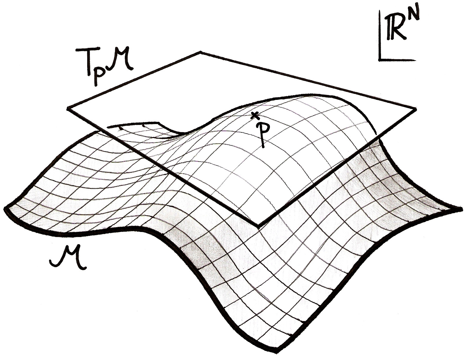
Figure 4: A manifold ${\cal M}$ embedded in $\mathbb{R}^{N}$. The point $p$ belongs to the manifold, and the plane tangent to ${\cal M}$ at $p$ is the tangent space $T_{p}{\cal M}$. In this drawing, we take $N=3$ and the manifold is two-dimensional. The grid was added to emphasize the fact that the manifold looks, locally, like a plane $\mathbb{R}^{2}$.

Given a vector space, it is natural to endow it with a scalar product, allowing one to compute norms of vectors and angles between vectors. Since a manifold ${\cal M}$ has a tangent space at each point, one would like to define a scalar product in the tangent space at each point of ${\cal M}$; a metric does precisely this job.

Definition.

A (Riemannian) metric $g$ on ${\cal M}$ is the data of a scalar product in each tangent space of ${\cal M}$, such that this scalar product varies smoothly on ${\cal M}$ [42]. More precisely, a metric is a symmetric, positive-definite, smooth tensor field

$$g:{\cal M}\rightarrow T^{2}({\cal M}):p\mapsto g_{p},$$ (3.1)

where $g_{p}$ is the aforementioned scalar product in $T_{p}{\cal M}$:

$$g_{p}:T_{p}{\cal M}\times T_{p}{\cal M}\rightarrow\mathbb{R}:(v,w)\mapsto g_{p}(v,w).$$ (3.2)

The requirements of symmetry and positive-definiteness ensure that $g_{p}$ satisfies all the standard properties of a scalar product. This definition can be extended to pseudo-Riemannian metrics, that is, symmetric tensor fields such as (3.1) that are not necessarily positive-definite. In particular, we will see below that $d$-dimensional Minkowski space-time is the manifold $\mathbb{R}^{d}$ endowed with the pseudo-Riemannian metric (3.9).

3.1.2 Examples

To illustrate concretely the above definition, let us consider a few simple examples of metrics on the manifold ${\cal M}=\mathbb{R}^{2}$. We can endow this manifold with global (Cartesian) coordinates $(x,y)$ such that any point $p\in\mathbb{R}^{2}$ is identified with its pair of coordinates. Our first example is the Euclidean metric, whose expression in Cartesian coordinates is

$$g=dx^{2}+dy^{2}.$$ (3.3)

To explain the meaning of this notation, let us pick a point $(x,y)$ in $\mathbb{R}^{2}$ and two vectors $v$ and $w$ at that point, with respective components $(v_{x},v_{y})$ and $(w_{x},w_{y})$. Their scalar product is given by (3.2), i.e.

$$g_{(x,y)}(v,w)=\left(dx^{2}+dy^{2}\right)\left[(v_{x},v_{y}),(w_{x},w_{y})\right].$$ (3.4)

By definition, upon acting on a vector, $dx$ gives the $x$-component of this vector. (In the standard language of differential geometry, $dx$ is the differential of $x$, that is, the one-form dual to the vector field $\partial/\partial x$ associated with the coordinate $x$ on $\mathbb{R}^{2}$.) The notation $dx^{2}$ is then understood as the operation which, upon acting on two vectors, gives the product of their components along $x$. A similar definition holds for $dy$ and $dy^{2}$, except that they, of course, give $y$-components of vectors. Applying these rules to (3.4), we find that the metric (3.3) defines the standard Euclidean scalar product,

$$g_{(x,y)}(v,w)=v_{x}w_{x}+v_{y}w_{y}.$$ (3.5)

Of course, one can define more generally the Euclidean metric on $\mathbb{R}^{d}$ to be $g=(dx_{1})^{2}+\cdots+(dx_{d})^{2}$ in terms of Cartesian coordinates.

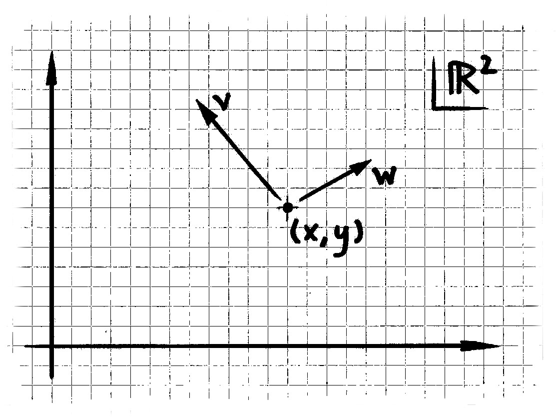
Figure 5: The plane $\mathbb{R}^{2}$ and the Cartesian coordinates used to label its points. A point with coordinates $(x,y)$ is also represented, and $v$, $w$ are two vectors at that point. Their scalar product with respect to the Euclidean metric (3.3) is given by (3.5).

A slightly less trivial example of metric on $\mathbb{R}^{2}$ is given by

$$g_{(x,y)}=\frac{dx^{2}+dy^{2}}{(1+x^{2}+y^{2})^{2}},$$ (3.6)

where $(x,y)$ is the point at which the metric is evaluated. If then $v$ and $w$ are two vectors at $(x,y)$, with the same components as before, their scalar product with respect to this new metric is

$$g_{(x,y)}(v,w)=\frac{v_{x}w_{x}+v_{y}w_{y}}{(1+x^{2}+y^{2})^{2}},$$

where we have used once more the rule saying that $dx$ (resp. $dy$), upon acting on a vector, gives the $x$-component (resp. $y$-component) of the vector. By contrast to the Euclidean scalar product (3.5), this expression depends explicitly on the point $(x,y)$. In other words, if we take two families of vectors on $\mathbb{R}^{2}$ with constant components $(v_{x},v_{y})$ and $(w_{x},w_{y})$ at each point of the plane, their scalar product will vary as we move on $\mathbb{R}^{2}$.

Of course, the metric (3.6) that we picked was chosen for illustrative purposes only: any positive function on $\mathbb{R}^{2}$ multiplying $dx^{2}+dy^{2}$ would give a (generally position-dependent) Riemannian metric on $\mathbb{R}^{2}$. More generally, any position-dependent, real quadratic combination of $dx$’s and $dy$’s,

$$A(x,y)dx^{2}+2B(x,y)dxdy+C(x,y)dy^{2},$$ (3.7)

is a Riemannian metric on $\mathbb{R}^{2}$ as long as $A$ and $AC-B^{2}$ are everywhere positive. If $v$ and $w$ are two vectors at $(x,y)$ with the same components as before, their scalar product with respect to the metric (3.7) is $A(x,y)v_{x}w_{x}+2B(x,y)v_{x}w_{y}+C(x,y)v_{y}w_{y}$. Again, the generalization of these considerations to $\mathbb{R}^{d}$ is straightforward: in terms of Cartesian coordinates $x_{1}$,…,$x_{d}$, the most general Riemannian metric on $\mathbb{R}^{d}$ takes the form $g_{ij}(x_{1},...,x_{d})dx_{i}dx_{j}$ (with implicit summation over $i,j=1,...,d$), where $(g_{ij})$ is a symmetric, positive-definite matrix at each point.

3.1.3 Angles and conformal transformations

Metrics can be used to define norms and angles on tangent spaces of a manifold. Indeed, suppose we are given a manifold ${\cal M}$ endowed with a metric $g$. Let $p$ be a point in ${\cal M}$ and let $v$ be a tangent vector of ${\cal M}$ at $p$. Then, the norm of $v$ is naturally defined to be $\|v\|\equiv\left[g_{p}(v,v)\right]^{1/2}$. Furthermore, if $v$ and $w$ are two vectors at $p$, the angle $\theta$ between them is defined (up to a sign) by

$$\cos\theta\equiv\frac{g_{p}(v,w)}{\|v\|\cdot\|w\|}.$$

Note that this definition is blind to the local normalization of the metric. Indeed, suppose we define two metrics $g$ and $g^{\prime}$ on ${\cal M}$, such that

$$\left(g^{\prime}\right)_{p}=\Omega(p)\cdot g_{p}\quad\forall\,p\in{\cal M},$$

where $\Omega$ is some smooth, positive real function on ${\cal M}$. In other words, let us assume that $g$ and $g^{\prime}$ are proportional, the proportionality factor being position-dependent. Then, these two metrics define the same angles. The proof is elementary: if $v$ and $w$ are two vectors at $p\in{\cal M}$, then the cosine of the angle between these vectors is

$$\frac{g_{p}(v,w)}{\left[g_{p}(v,v)\,g_{p}(w,w)\right]^{1/2}}=\frac{\Omega(p)g_{p}(v,w)}{\left[\Omega(p)g_{p}(v,v)\,\Omega(p)g_{p}(w,w)\right]^{1/2}}=\frac{g^{\prime}_{p}(v,w)}{\left[g^{\prime}_{p}(v,v)\,g^{\prime}_{p}(w,w)\right]^{1/2}},$$

which is obviously independent of whether we choose to use the metric $g$ or the metric $g^{\prime}$. This observation will be crucial in the following pages.

Given a manifold ${\cal M}$, it is natural to wonder what modifications ${\cal M}$ may undergo, such that these modifications “preserve the structure” of ${\cal M}$. To answer this question, we must specify precisely what is the structure we wish to preserve. Clearly, a first feature we would like to preserve when deforming ${\cal M}$ is its local Euclidean structure. This leads to the notion of diffeomorphisms: by definition, a diffeomorphism of a manifold ${\cal M}$ is a smooth, invertible map $\phi:{\cal M}\rightarrow{\cal M}$ such that the inverse map $\phi^{-1}$ be smooth as well. In this sentence, the word “smooth” means “that preserves the local Euclidean structure in a continuous and differentiable way”. In heuristic terms, a diffeomorphism of ${\cal M}$ is a smooth, invertible deformation of ${\cal M}$ when the latter is seen as a rubber space.

Figure 6: A diffeomorphism of the sphere. The arrows represent how points of the sphere move as the diffeomorphism is applied. Under the action of the diffeomorphism, points are shuffled, shapes are distorted, but the motion is smooth, preserving the local Euclidean structure of the manifold.

Suppose now we pick a manifold ${\cal M}$ endowed with a metric $g$, and consider a diffeomorphism $\phi:{\cal M}\rightarrow{\cal M}$ of that manifold. Since the diffeomorphism is a deformation of ${\cal M}$, it will in general affect distances and angles on ${\cal M}$; in other words, a general diffeomorphism does not preserve the metric on ${\cal M}$ and maps the original metric $g$ on some new metric $g^{\prime}$. (In precise terms, what we call the transformed metric is the pull-back of $g$ by $\phi$, that is, $g^{\prime}\equiv\phi^{*}g$.) This gives a motivation for defining certain subclasses of diffeomorphisms that preserve some part (or the entirety) of the metric structure, i.e. diffeomorphisms for which the new metric $g^{\prime}$ has certain properties in common with the first metric $g$.

Definition.

A conformal transformation of ${\cal M}$ is a diffeomorphism $\phi:{\cal M}\rightarrow{\cal M}$ such that the original metric $g$ and the transformed metric $g^{\prime}$ define the same angles (possibly up to signs).

Given the property, shown above, that proportional metrics define identical angles (possibly up to signs), it is easy to write down an explicit formula for what we mean by a conformal transformation: it is a diffeomorphism for which the transformed metric $g^{\prime}$ is related to the original metric $g$ as

$$g^{\prime}_{p}=\Omega(p)g_{p}\quad\forall\,p\in{\cal M},$$ (3.8)

where $\Omega$ is some smooth, positive function on ${\cal M}$. When $\Omega(p)=1$ for all $p$ in ${\cal M}$, we say that the diffeomorphism $\phi$ is an isometry: it preserves not only the angles, but also the norms defined by the metric $g$. Of course, conformal transformations and isometries can also be defined for pseudo-Riemannian metrics.

Remark.

We are now equipped with the tools needed to restate in differential-geometric terms the definition of the Lorentz and Poincaré groups, originally described in subsection 1.2. Namely, define $d$-dimensional Minkowski space to be the manifold $\mathbb{R}^{d}$ endowed with a pseudo-Riemannian metric $g$ such that there exist global coordinates $(x^{\mu})$ on $\mathbb{R}^{d}$ in which the metric takes the form

$$g=\eta_{\mu\nu}dx^{\mu}dx^{\nu}=-(dx^{0})^{2}+dx^{i}dx^{i},\quad i=1,...,d-1,$$ (3.9)

with $(\eta_{\mu\nu})$ the Minkowski metric matrix written in (1.5) for the case $d=4$. In the language of subsection 1.1, the coordinates $(x^{\mu})$ are those of an inertial frame. Then the isometry group of this manifold is precisely the Poincaré group in $d$ dimensions, acting on $\mathbb{R}^{d}$ according to (1.8), and the stabilizer for this action is the Lorentz group $\mathrm{O}(d-1,1)$. From this viewpoint, the property (1.6) of invariance of the interval is simply the defining criterion for the transformation to be an isometry.

3.2 Conformal transformations of the plane

To illustrate the definition of conformal transformations in the simplest possible case, let us consider the plane $\mathbb{R}^{2}$ endowed with the Euclidean metric (3.3). To make things technically simpler, we see $\mathbb{R}^{2}$ as the complex plane $\mathbb{C}$ and introduce a complex coordinate $z\equiv x+iy$, in terms of which the metric (3.3) becomes $g=dzd\bar{z}$ (with $\bar{z}$ the complex conjugate of $z$). Then a generic diffeomorphism is a map

$$\phi:\mathbb{C}\rightarrow\mathbb{C}:z\mapsto Z(z,\bar{z}),$$ (3.10)

where the function $Z$ generally depends on both $z$ and $\bar{z}$. Demanding that $\phi$ be a conformal transformation imposes certain restrictions on this function, which we now work out.

Since $\phi$ maps $z$ on $Z$ and since the metric $g$ is just $dzd\bar{z}$, it is natural that the transformed metric be

$$g^{\prime}_{z}=\left.dZd\bar{Z}\right|_{z},$$ (3.11)

where the subscript $z$ means that both sides are evaluated at the point $z$. (This is just the definition $g^{\prime}=\phi^{*}g$ applied to (3.10).) Here the differential of $Z$ is

$$\left.dZ\right|_{z}=\frac{\partial Z}{\partial z}dz+\frac{\partial Z}{\partial\bar{z}}d\bar{z}.$$

Plugging this expression (and its complex conjugate) in (3.11), we find

$$g^{\prime}_{z}=\frac{\partial Z}{\partial z}\frac{\partial\bar{Z}}{\partial z}dz^{2}+\frac{\partial Z}{\partial\bar{z}}\frac{\partial\bar{Z}}{\partial\bar{z}}d\bar{z}^{2}+\left[\frac{\partial Z}{\partial z}\frac{\partial\bar{Z}}{\partial\bar{z}}+\frac{\partial Z}{\partial\bar{z}}\frac{\partial\bar{Z}}{\partial z}\right]dzd\bar{z}.$$

According to the definition surrounding eq. (3.8), requiring that $\phi$ be a conformal transformation amounts to demanding that this expression be proportional to $g_{z}=dzd\bar{z}$. The terms involving $dz^{2}$ or $d\bar{z}^{2}$ must therefore vanish, which is the case if and only if

$$\frac{\partial Z}{\partial\bar{z}}=0\quad\text{or}\quad\frac{\partial Z}{\partial z}=0.$$ (3.12)

In other words, the function $Z$ must depend either only on $z$, or only on $\bar{z}$. The latter possibility represents conformal transformations that change the orientation of $\mathbb{R}^{2}$ (they map an angle $\theta$ on an angle $-\theta$), and we will discard them from now on. Thus, a diffeomorphism (3.10) is an orientation-preserving conformal transformation of $\mathbb{R}^{2}$ provided $Z$ is a function of $z$ only, that is, a meromorphic function. Furthermore, locally, any such function is admissible.

Of course, this is not the end of the story since (3.10) must be a smooth bijection. This restricts the form of $Z(z)$ even further. To begin with, $Z(z)$ must be regular, so $Z(z)$ must be an analytic function

$$Z(z)=A+Bz+Cz^{2}+Dz^{3}+\cdots.$$ (3.13)

The zeros of $Z(z)$ are the points that are mapped on the origin $Z=0$. Since $Z(z)$ must be an injective map, there can be only one such zero, say $z^{*}$. If this zero is degenerate, then the map $Z(z)$ will not be injective in a neighbourhood of that zero. (If $z$ is sufficiently close to $z^{*}$ and if $z^{*}$ is a zero of $Z(z)$ with order $n>1$, then $z$ is mapped by $Z$ on $n$ different points, and $Z(z)$ cannot be injective.) Thus, in (3.13), the coefficients of all powers of $z$ higher than one must vanish, i.e. $C=D=0$, etc. In other words, the function $Z(z)$ must be linear in $z$. Finally, requiring $Z(z)$ to be surjective imposes that the coefficient of the $z$-linear term be non-zero. We conclude that all conformal transformations of the plane are of the form

$$Z(z)=az+b,\quad\text{with }a,\,b\in\mathbb{C}\quad\text{and }a\neq 0.$$ (3.14)

These transformations naturally split in three classes:

Translations	$z\mapsto z+b$,	$b\in\mathbb{C}$;
Rotations	$z\mapsto e^{i\theta}z$,	$\theta\in\mathbb{R}$;
Dilations	$z\mapsto e^{-\chi}z$,	$\chi\in\mathbb{R}$.

We will see in the next subsection that these transformations may also be seen as (a subclass of) conformal transformations of the sphere.

Before going further, let us note one important detail: in deriving the set of conformal transformations (3.14), the fact that the metric $g$ on $\mathbb{C}$ was the Euclidean metric (3.3) played a minor role. Indeed, we would have obtained the exact same set of transformations for any metric of the form $\Omega(z,\bar{z})dzd\bar{z}$ on the plane, since conformal transformations are blind to the multiplication of metrics by (positive) functions. The only crucial point was that the metric be proportional to $dzd\bar{z}$, since it is this property that led to the condition (3.12). The further restrictions leading to (3.14), on the other hand, originated from topological (hence metric-independent) considerations. These observations will be essential in the following subsection.

3.3 Conformal transformations of the sphere

We now turn to the main goal of this section: the classification of conformal transformations of the sphere $S^{2}$. By definition, the latter is a two-dimensional manifold consisting of all points with Cartesian coordinates $(x_{1},x_{2},x_{3})$ in $\mathbb{R}^{3}$ such that $x_{1}^{2}+x_{2}^{2}+x_{3}^{2}=r^{2}$, where $r$ is some fixed (positive) radius. (The notation $S^{2}$ is usually reserved for the unit sphere, with radius $r=1$, but here we will denote any sphere by $S^{2}$, regardless of its radius.)

3.3.1 Stereographic coordinates

The standard way to locate points on a sphere of radius $r$ relies on polar coordinates $\theta\in[0,\pi]$ and $\varphi\in[0,2\pi)$ defined by

$$\left\{\begin{array}[]{ccl}x_{1}&=&r\sin\theta\cos\varphi,\\ x_{2}&=&r\sin\theta\sin\varphi,\\ x_{3}&=&r\cos\theta\end{array}\right.$$

for any point $(x_{1},x_{2},x_{3})$ belonging to the sphere.

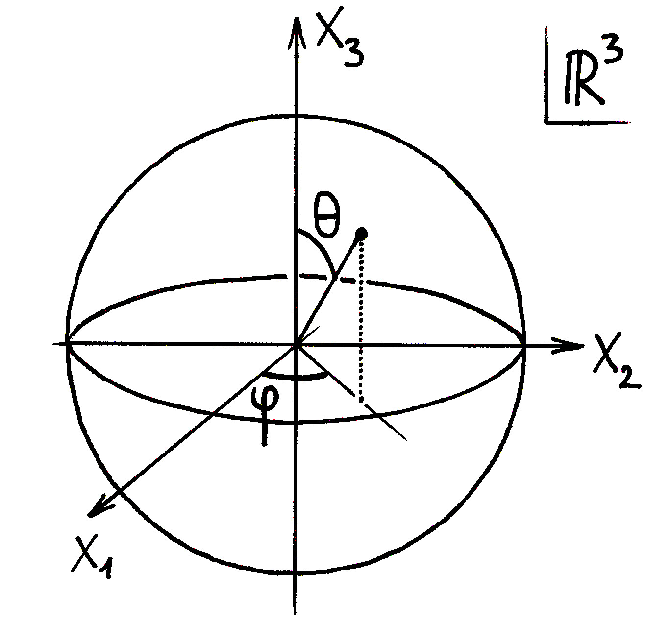
Figure 7: A sphere embedded in $\mathbb{R}^{3}$, and the polar coordinates $\theta$, $\varphi$ used to label its points.

In the present case, however, it will be more convenient to use so-called stereographic coordinates, which will simplify the treatment of conformal transformations. These coordinates are defined as follows. Consider a point $(x_{1},x_{2},x_{3})$ on the sphere, different from the south pole $(0,0,-r)$. Then, there exists a unique straight line in $\mathbb{R}^{3}$ passing through that point and the south pole. Explicitly, all points belonging to this line have coordinates $(y_{1},y_{2},y_{3})$ of the form

$$\left\{\begin{array}[]{rcl}y_{1}&=&tx_{1},\\ y_{2}&=&tx_{2},\\ y_{3}&=&t(x_{3}+r)-r\end{array}\right.$$ (3.15)

where $t$ is a parameter running over all real values. (The point corresponding to $t=0$ is the south pole, while $t=1$ corresponds to $(x_{1},x_{2},x_{3})$.) The straight line so obtained crosses the equatorial plane $\left\{(x_{1},x_{2},0)|x_{1},x_{2}\in\mathbb{R}\right\}$ at exactly one point, called the stereographic projection of $(x_{1},x_{2},x_{3})$ through the south pole. The coordinates $(x^{\prime}_{1},x^{\prime}_{2},0)$ of this projection are obtained by setting $y_{3}=0$ in eq. (3.15), that is, by taking $t=r/(r+x_{3})$, which gives

$$x^{\prime}_{1}=\frac{r\,x_{1}}{r+x_{3}},\quad x^{\prime}_{2}=\frac{r\,x_{2}}{r+x_{3}}.$$ (3.16)

We will refer to $x^{\prime}_{1}$ and $x^{\prime}_{2}$ as the stereographic coordinates on the sphere. They can be combined into a single complex coordinate

$$z\equiv\frac{x^{\prime}_{1}+ix^{\prime}_{2}}{r}=\frac{x_{1}+ix_{2}}{r+x_{3}},$$ (3.17)

which is related to polar coordinates through

$$z=e^{i\varphi}\tan(\theta/2).$$ (3.18)

For future reference, note that the inverse of relation (3.17) gives $(x_{1},x_{2},x_{3})$ in terms of $z$ and $\bar{z}$ as

$$x_{1}=r\frac{z+\bar{z}}{1+z\bar{z}},\quad x_{2}=\frac{r}{i}\frac{z-\bar{z}}{1+z\bar{z}},\quad x_{3}=r\frac{1-z\bar{z}}{1+z\bar{z}},$$ (3.19)

where we used the fact that $x_{1}^{2}+x_{2}^{2}+x_{3}^{2}=r^{2}$. Of course, we could have carried out a parallel construction by projecting points of the sphere on the equatorial plane through the north pole; this would have given formulas analogous to (3.16) and (3.17), but with $r+x_{3}$ replaced by $r-x_{3}$.

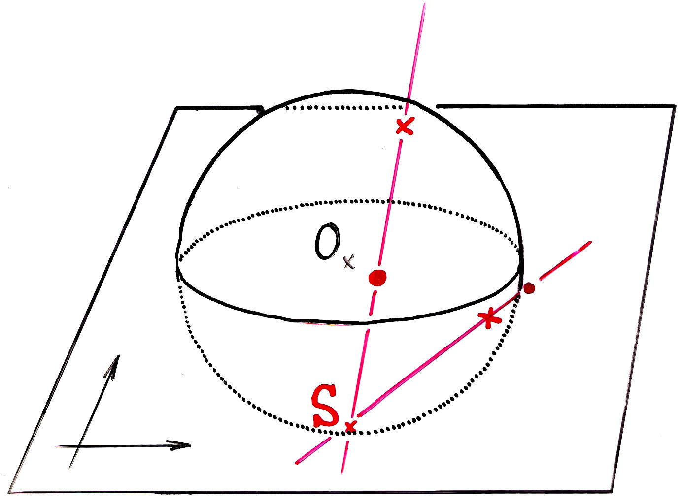
Figure 8: The stereographic projection of a sphere centered at $O$ through the south pole $S$. The two red crosses are points belonging to the sphere; the projection maps those points on the two red dots on the equatorial plane, following straight lines parametrized by eq. (3.15). The coordinates $(x^{\prime}_{1},x^{\prime}_{2},0)$ of the projection of a point $(x_{1},x_{2},x_{3})$ are given by (3.16).

The stereographic projection is a concrete illustration of the fact that a sphere is locally the same as a plane: any point on the sphere, other than the south pole, can be projected to the equatorial plane through the south pole. Points that are close to the north pole get projected near the origin $z=0$; the whole northern hemisphere is projected in the unit disc $|z|<1$, and the equator is left fixed by the projection, corresponding to the unit circle $|z|=1$. Points belonging to the southern hemisphere, on the other hand, are projected outside of the unit disc. In particular, points located near the south pole are projected far from the origin, at large values of $|z|$: as points get closer to the south pole, they get projected further and further away. In fact, one may view the infinitely remote point on the plane, the “point at infinity” $z=\infty$, as the projection of the south pole itself. (Of course, the actual projection of the south pole is ill-defined, so the point at infinity does not have a well-defined argument.) We conclude that the sphere is diffeomorphic to a plane, up to a point. More precisely,

$$S^{2}\cong\mathbb{C}\cup\{\text{point at infinity}\}=\mathbb{C}\cup\{z=\infty\}.$$ (3.20)

The representation of the sphere as a plane to which one adds the point at infinity is called the Riemann sphere [43]. This relation hints that some of the results derived above for conformal transformations of the plane should be applicable to the sphere as well. In order to see concretely if this is the case, we first need to express the metric of a sphere in terms of the coordinate $z$.

3.3.2 The metric on a sphere in stereographic coordinates

The natural metric on a sphere follows from the definition of a sphere as a submanifold of $\mathbb{R}^{3}$. Namely, endowing $\mathbb{R}^{3}$ with the Euclidean metric $dx_{1}^{2}+dx_{2}^{2}+dx_{3}^{2}$, the metric on the sphere is simply

$$g=\left.\left(dx_{1}^{2}+dx_{2}^{2}+dx_{3}^{2}\right)\right|_{x_{1}^{2}+x_{2}^{2}+x_{3}^{2}=r^{2}}.$$ (3.21)

To express this metric in terms of stereographic coordinates, we use formula (3.17), from which it follows that the differential of $z$ is

$$dz=\frac{(dx_{1}+idx_{2})(r+x_{3})-(x_{1}+ix_{2})dx_{3}}{(r+x_{3})^{2}}.$$

On the sphere defined by $x_{1}^{2}+x_{2}^{2}+x_{3}^{2}=r^{2}$, the differentials of $x_{1}$, $x_{2}$ and $x_{3}$ satisfy the relation $x_{1}dx_{1}+x_{2}dx_{2}+x_{3}dx_{3}=0$, which can then be used to show that

$$dzd\bar{z}=\frac{1}{(r+x_{3})^{2}}\left.\left(dx_{1}^{2}+dx_{2}^{2}+dx_{3}^{2}\right)\right|_{x_{1}^{2}+x_{2}^{2}+x_{3}^{2}=r^{2}}.$$

In the last term of this expression we recognize the metric (3.21) on the sphere, whose expression in terms of $z$ thus becomes

$$g_{z}=(r+x_{3})^{2}dzd\bar{z}=\frac{4r^{2}}{(1+z\bar{z})^{2}}dzd\bar{z},$$ (3.22)

where we used the third relation of (3.19) to write $x_{3}$ as a function of $z$ and $\bar{z}$. This metric is position-dependent, since it explicitly depends on $z$. In fact, up to the factor $4r^{2}$, it is precisely the metric (3.6) that we took as an example earlier on, written in terms of $z=x+iy$. The only subtlety is that, in contrast to (3.6) where $x$ and $y$ only take finite values, expression (3.22) must be understood as a metric on the Riemann sphere, where $|z|$ may be infinite.

Crucially, the metric (3.22) is proportional to the Euclidean metric $dzd\bar{z}$, which implies that, as far as conformal transformations are concerned, we can simply repeat the derivation carried out in subsection 3.2 for the plane. More precisely, if we demand that a diffeomorphism $\phi:\mathbb{C}\cup\{z=\infty\}\rightarrow\mathbb{C}\cup\{z=\infty\}:z\mapsto Z(z,\bar{z})$ be a conformal transformation, the arguments that led to (3.12) remain true and the function $Z$ must depend either only on $z$, or only on $\bar{z}$. The latter choice corresponds to transformations that do not preserve the orientation of the sphere, so we will ignore them. Thus, any orientation-preserving conformal transformation of the sphere is a meromorphic function of the form $z\mapsto Z(z)$, and locally on the sphere this is all we can say.

Globally, of course, this is not yet the end of the story, since we must further require that the function $Z(z)$ be a diffeomorphism of the sphere $-$ that is, a diffeomorphism of the plane $\mathbb{C}$ with the point at infinity added as in (3.20). This point will play a key role. Indeed, requiring that $Z(z)$ be regular on $\mathbb{C}\cup\{z=\infty\}$ no longer means that $Z(z)$ is analytic as in (3.13); rather, $Z(z)$ now may (and should) have at least one pole, at $z^{*}$ say, corresponding to the point that is mapped to the south pole $Z(z^{*})=\infty$. Thus, $Z(z)$ should now be a rational function of the general form

$$Z(z)=\frac{A+Bz+Cz^{2}+Dz^{3}+\cdots}{A^{\prime}+B^{\prime}z+C^{\prime}z^{2}+D^{\prime}z^{3}+\cdots},$$

where the roots of the numerator (resp. denominator) correspond to the points that are mapped on the origin $Z=0$ (resp. the point at infinity $Z=\infty$), i.e. on the north pole (resp. the south pole). Since $Z(z)$ must be an injective map, there must be one, and only one, point that is mapped to the north pole, and also exactly one other point that is mapped to the south pole. As in subsection 3.2, this requires that both the numerator and the denominator be linear functions of $z$. We can thus write any orientation-preserving conformal transformation of the Riemann sphere as

$$\boxed{Z(z)=\frac{az+b}{cz+d},}$$ (3.23)

where $a$, $b$, $c$ and $d$ are complex numbers. Requiring this map to be surjective finally imposes that

$$\text{det}\begin{pmatrix}a&b\\ c&d\end{pmatrix}\neq 0.$$ (3.24)

This is the classification of conformal transformations of the sphere that we were looking for. Such transformations are also called Möbius transformations. They obviously contain the set of conformal mappings (3.14) of the plane, so that translations of $z$, rotations and dilations also represent conformal transformations of the sphere. However, there is now an additional two-parameter family of transformations of the form

$$z\mapsto-b^{2}/z,\quad b\in\mathbb{C}^{*},$$

corresponding to so-called special conformal transformations [11, 12]. Such transformations map the north pole on the south pole, and vice-versa. Any conformal transformation of the sphere can be obtained as the composition of a special conformal transformation, a translation, a rotation and a dilation (possibly in a different order).

By construction, conformal transformations span a group, so it is worthwile to investigate the group structure of the set of Möbius transformations. Clearly, formula (3.23) is blind to the overall normalization of the matrix in (3.24), since multiplying all entries of the matrix by the same non-zero complex number leads to the same transformation (3.23). We can thus assume, without loss of generality, that the non-zero determinant (3.24) is actually one, i.e. that the matrix $\begin{pmatrix}a&b\\ c&d\end{pmatrix}$ belongs to $\mathrm{SL}(2,\mathbb{C})$. Furthermore, two matrices in $\mathrm{SL}(2,\mathbb{C})$ that differ only by their sign define the same conformal transformation, so the group of all non-degenerate transformations of the form (3.23) is actually isomorphic to the quotient

$$\mathrm{SL}(2,\mathbb{C})/\mathbb{Z}_{2}.$$ (3.25)

In other words, according to (2.22), the set of orientation-preserving conformal transformations of the sphere forms a group isomorphic to the connected Lorentz group in four dimensions! At this stage, this relation appears just as a coincidence of group theory: there seems to be no relation whatsoever between the Möbius transformations (3.23) and the original definition of the Lorentz group as a matrix group acting on $\mathbb{R}^{4}$. The purpose of the next section will be to show that this apparent coincidence actually has a geometric origin, rooted in the structure of light-like straight lines in Minkowski space-time.

3.4 An aside: conformal field theories in two dimensions

In the two previous subsections we have seen that any (orientation-preserving) conformal transformation of a two-dimensional manifold with a conformally flat metric $\propto dzd\bar{z}$ can be written as a meromorphic function $z\mapsto Z(z)$. Demanding that $Z(z)$ be a bijection of the manifold imposes certain restrictions on the function $Z$, leading to (3.14) in the case of the plane, and (3.23) in the case of the sphere. However, in physical applications, it is often the case that “global” requirements such as bijectivity play a minor role. This is particularly true in the case of local quantum field theories, whose properties are mostly determined by local (as opposed to global) considerations.

This feature is of central importance in the context of conformal field theories in two dimensions [11, 12]. By definition, a conformal field theory in $d$ dimensions is a quantum field theory, defined on a $d$-dimensional manifold ${\cal M}$ endowed with some metric $g$, that is invariant under conformal transformations of ${\cal M}$. In the case ${\cal M}=S^{2}$, with a metric proportional to $dzd\bar{z}$ in terms of stereographic coordinates, this leads to theories that are invariant under all Möbius transformations (3.23). However, the actual set of infinitesimal symmetries of such theories (i.e. symmetries found without taking global issues into account) turns out to be much, much larger than the finite-dimensional group (3.25). Indeed, since global requirements such as bijectivity play a secondary role, conformal field theories in two dimensions turn out to be invariant under all transformations that can be written locally as $z\mapsto Z(z)$, where $Z(z)$ is any meromorphic function. This leads to an infinite-dimensional symmetry algebra that constrains such theories in a extremely powerful way [46]. For instance, when combined with an additional symmetry property called “modular invariance”, conformal invariance of a two-dimensional field theory implies a universal formula for the entropy of that theory, known as the Cardy formula [47]. We will briefly return to conformal field theories in the conclusion of these notes.

4 Lorentz group and celestial spheres

So far we have seen that the connected Lorentz group in four dimensions, $L_{+}^{\uparrow}=\mathrm{SO}(3,1)^{\uparrow}$, is isomorphic to the quotient $\mathrm{SL}(2,\mathbb{C})/\mathbb{Z}_{2}$. We have also shown that the latter arises as the group of orientation-preserving conformal transformations of the sphere. However, at this stage, the relation between the Lorentz group and the sphere appears as a mere coincidence. In particular, since the original Lorentz group is defined by its linear action on a four-dimensional space, there is no reason for it to have anything to do with certain non-linear transformations of a two-dimensional manifold such as the sphere. The purpose of this section is to establish this missing link. This will require first defining a notion of “celestial spheres” in Minkowski space-time (subsection 4.1), and then computing the action of Lorentz transformations on such spheres (subsection 4.2). Subsection 4.3 is devoted to the analysis of the somewhat counterintuitive action of Lorentz boosts in terms of celestial spheres. Our approach is motivated by the notion of “asymptotic symmetries” in gravity [14], and will rely on a specific choice of coordinates that simplifies the description of null infinity in Minkowski space-time. The results as such are well known, and coordinate-independent $-$ see for instance [3, 4]. It should be noted that similar relations exists also in other space-time dimensions. For instance, in $d=3$ dimensions, the connected Lorentz group $\mathrm{SO}(2,1)^{\uparrow}$ acts on the celestial circles at null infinity through projective transformations spanning a group $\mathrm{SL}(2,\mathbb{R})/\mathbb{Z}_{2}$, in accordance with the isomorphism (2.12). In this section, however, we will restrict our attention to the four-dimensional case.

4.1 Notion of celestial spheres

As explained in section 1, inertial observers in special relativity live in Minkowski space-time, which may be seen as the vector space $\mathbb{R}^{4}$. Inertial coordinates consist of one time coordinate $t$ or $x^{0}=ct$, and three Cartesian space coordinates $(x^{1},x^{2},x^{3})=(x^{i})$. (Latin indices run over the values $1$, $2$, $3$.) Given such coordinates, there is a natural way to define a corresponding family of spheres. Namely, one may describe the spatial location of an event in terms of spherical, rather than Cartesian, coordinates, defined as

$$r\equiv\sqrt{(x^{1})^{2}+(x^{2})^{2}+(x^{3})^{2}}=\sqrt{x^{i}x^{i}}\quad\text{and}\quad z\equiv\frac{x^{1}+ix^{2}}{r+x^{3}},$$ (4.1)

where points on the sphere of radius $r$ are labelled by the stereographic coordinates (3.17). In particular, the spatial coordinates $x^{i}=x_{i}$ take the form (3.19) when expressed in terms of $z$ and $\bar{z}$. Note that the parity transformation defined by the matrix (1.16) acts on the coordinate $z$ according to $z\mapsto-1/\bar{z}$.

For each non-zero $r$, we thus have a spatial sphere naturally associated with the inertial coordinates $(x^{0},x^{1},x^{2},x^{3})$. Since Lorentz transformations relate different sets of inertial coordinates through linear transformations $x\mapsto x^{\prime}=\Lambda\cdot x$, one might hope that the rewriting of these transformations in terms of spherical coordinates (4.1) could give rise to a “nice” action of the Lorentz group on spatial spheres, one that would make the relation to conformal transformations more apparent. This is not quite the case, however; roughly speaking, the “celestial sphere” that we actually wish to define should be the sphere that an inertial observer looks at. This is not achieved by the sphere of radius $r$ defined by (4.1), because radial, ingoing light-rays emitted by the sphere need a non-zero time $r/c$ to get from the sphere to the origin at $r=0$ (which we take to be the position of the observer). Thus, we need to work a little more: we must somehow combine space and time coordinates so as to take into account the finite velocity of light, and define the celestial sphere seen by an observer at some moment of time as an object living in the past.

The argument just outlined hints at the right definition of what we would like to call a “celestial sphere”. Indeed, consider a radial light ray whose trajectory in space-time is described by

$$r=r_{0}\pm ct=r_{0}\pm x^{0},\quad z=\text{constant}.$$

In particular, an ingoing radial light ray satisfies $r=r_{0}-ct$ where $r_{0}$ is some strictly positive initial radius. Along the trajectory of this light ray, the quantity

$$u\equiv ct+r=x^{0}+r$$ (4.2)

is constant; it represents the time at which the observer located at $r=0$ sees the light ray. One can thus parametrize the time of emission of ingoing radial light rays by the value of $u$. Instead of using coordinates $(x^{0},r,z)$ to locate events in space-time, one may then use the Bondi coordinates $(u,r,z)$, in which case $u$ plays the role of a time coordinate and is called advanced time. The situation can be depicted as follows:

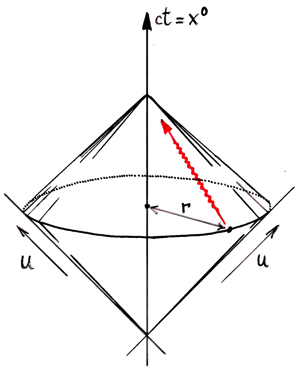
Figure 9: The Bondi coordinates $u$ and $r$ in Minkowski space-time. The time coordinate $x^{0}=ct$ points upwards. The wavy red line represents an incoming radial light ray, emitted from some non-zero distance $r$ towards the observer located at $r=0$. The light ray moves along one of the generators of the light cone defined by $u=\text{cst}$. The figure represents three-dimensional space-time, so the circle of radius $r$ in this drawing would in fact be a sphere in our actual, four-dimensional, space-time. That sphere is spanned by the stereographic coordinate $z$ in (4.1).

In terms of Bondi coordinates, a sphere at constant $r>0$ and constant $u\in\mathbb{R}$ coincides with the sphere seen by an observer sitting at the origin $r=0$ at time $u$. We can then define the celestial sphere at time $u$ as the sphere located at an infinite distance, $r\rightarrow+\infty$, and at a fixed value of $u$. It is the sphere of all directions towards which an observer at $r=0$ can look [3], the reason for the name “celestial” being obvious in that context. (Celestial spheres are also sometimes called “heavenly spheres” [37].) Less obvious is the fact that this definition is the one needed to match Lorentz transformations and Möbius transformations, which will be the purpose of the next subsection. The region $\mathbb{R}\times S^{2}$ spanned by the coordinates $u$ and $z$ at $r\rightarrow+\infty$ is called past null infinity [14]: it consists of events located at an infinite distance from the observer, and it can be reached from the line $r=0$ by following a past-directed null vector, that is, a vector whose norm squared vanishes with respect to the Minkowski metric (3.9).

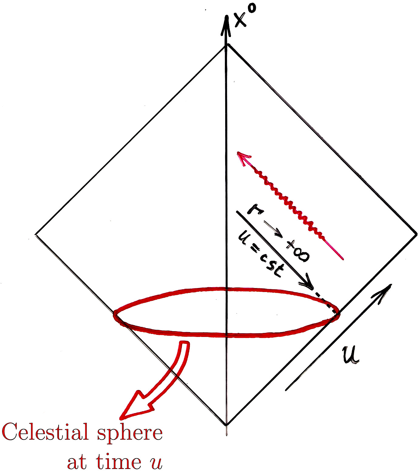
Figure 10: A schematic representation of celestial spheres. As in Fig. 9, the time coordinate $x^{0}$ points upwards and the wavy red line represents an incoming radial light ray. The picture represents three-dimensional space-time. Accordingly, the red circle at the bottom of the image would really be a sphere $-$ a celestial sphere $-$ in our four-dimensional space-time. Past null infinity is the cone on the lower half of the image; it is a manifold $\mathbb{R}\times S^{2}$ spanned by the advanced time $u$ and the stereographic coordinate $z$.

Remark.

In these notes we define celestial spheres by using a specific set of coordinates $(u,r,z)$ in Minkowski space-time. There also exists a different definition, according to which the celestial sphere associated with a point in space-time is the projective space of its (past) light-cone, that is, the set of past-directed null directions passing through that point [3]. In such terms, the celestial sphere at time $u$ that we defined above is the set of past-directed null directions through the point with Bondi coordinates $(r=0,u)$. (This could be any point in space-time since the Minkowski metric is invariant under all space-time translations.) This sphere can be thought of as the complex projective line $\mathbb{CP}^{1}\cong S^{2}$, and Lorentz transformations span the group $\mathrm{SL}(2,\mathbb{C})/\mathbb{Z}_{2}$ of its projective transformations $-$ which are nothing but Möbius transformations when seeing $\mathbb{CP}^{1}$ as a sphere $S^{2}$ [3]. The advantage of this projective viewpoint is that it is manifestly coordinate-independent, but we will not adopt this approach here. (See, however, the end of subsection 4.3.)

4.2 Lorentz transformations acting on celestial spheres

The Lorentz group is defined as the set of linear transformations $x\mapsto x^{\prime}=\Lambda\cdot x$ between coordinates of inertial observers in Minkowski space-time. In the previous subsection we have introduced new, non-inertial, Bondi coordinates $(u,r,z)$ associated with each choice of inertial coordinates $(x^{\mu})$. In order to find the action of the Lorentz group on Bondi coordinates, we must express both $x^{\prime}$ and $x$ in terms of the associated Bondi coordinates, then rewrite the relation $x^{\prime}=\Lambda\cdot x$ in Bondi coordinates and read off the Lorentz transformation properties of $(u,r,z)$. Since the relation between inertial coordinates and Bondi coordinates is non-linear, this procedure leads in general to cumbersome expressions for $(u^{\prime},r^{\prime},z^{\prime})$ in terms of $(u,r,z)$ and of the matrix elements ${\Lambda^{\mu}}_{\nu}$ of a Lorentz transformation. Fortunately, we are not actually interested in the general relation between $(u^{\prime},r^{\prime},z^{\prime})$ and $(u,r,z)$, but only in its limit $r\rightarrow+\infty$ with finite $u$. Provided Lorentz transformations preserve that limit (which is to be expected since they are linear in inertial coordinates), keeping $u^{\prime}$ finite, they correspond to well-defined transformations of past null infinity.

4.2.1 Transformation of the radial coordinate

Let us begin by computing the transformation law of the radial coordinate $r$ under Lorentz transformations. By definition, the (square of the) radial coordinate $r^{\prime}$ associated with the inertial coordinates $(x^{\prime\mu})$ is $r^{\prime 2}=(x^{\prime 1})^{2}+(x^{\prime 2})^{2}+(x^{\prime 3})^{2}$. If now we assume that the coordinates $x^{\prime\mu}$ are obtained by acting on certain coordinates $x^{\mu}$ with a Lorentz transformation $\Lambda$, we have $x^{\prime\mu}={{\Lambda}^{\mu}}_{\nu}x^{\nu}$ and

$$r^{\prime 2} = \left({\Lambda^{1}}_{0}x^{0}+{\Lambda^{1}}_{1}x^{1}+{\Lambda^{1}}_{2}x^{2}+{\Lambda^{1}}_{3}x^{3}\right)^{2}$$ (4.3)

$$+\left({\Lambda^{2}}_{0}x^{0}+{\Lambda^{2}}_{1}x^{1}+{\Lambda^{2}}_{2}x^{2}+{\Lambda^{2}}_{3}x^{3}\right)^{2}$$

$$+\left({\Lambda^{3}}_{0}x^{0}+{\Lambda^{3}}_{1}x^{1}+{\Lambda^{3}}_{2}x^{2}+{\Lambda^{3}}_{3}x^{3}\right)^{2}.$$

The next step consists in expressing the coordinates $x^{\mu}$ in terms of Bondi coordinates $(u,r,z)$ through relations (3.19) and (4.2). Taking the limit $r\rightarrow+\infty$ while keeping $u$ and $z$ fixed, the only terms that survive in the parentheses are those proportional to $r$, which gives

$$r^{\prime 2} = \left(-{\Lambda^{1}}_{0}r+{\Lambda^{1}}_{1}r\frac{z+\bar{z}}{1+z\bar{z}}+{\Lambda^{1}}_{2}\frac{r}{i}\frac{z-\bar{z}}{1+z\bar{z}}+{\Lambda^{1}}_{3}r\frac{1-z\bar{z}}{1+z\bar{z}}\right)^{2}$$

$$+\left(-{\Lambda^{2}}_{0}r+{\Lambda^{2}}_{1}r\frac{z+\bar{z}}{1+z\bar{z}}+{\Lambda^{2}}_{2}\frac{r}{i}\frac{z-\bar{z}}{1+z\bar{z}}+{\Lambda^{2}}_{3}r\frac{1-z\bar{z}}{1+z\bar{z}}\right)^{2}$$

$$+\left(-{\Lambda^{3}}_{0}r+{\Lambda^{3}}_{1}r\frac{z+\bar{z}}{1+z\bar{z}}+{\Lambda^{3}}_{2}\frac{r}{i}\frac{z-\bar{z}}{1+z\bar{z}}+{\Lambda^{3}}_{3}r\frac{1-z\bar{z}}{1+z\bar{z}}\right)^{2}+{\cal O}(r).$$

(In particular, in that limit, we may replace $x^{0}$ by $-r$.) Here the terms of order $r$ outside the parentheses are subdominant with respect to the terms of order $r^{2}$ coming from the parentheses. As the final touch, we take $\Lambda$ to be a proper, orthochronous Lorentz transformation, i.e. an element of the connected Lorentz group $L_{+}^{\uparrow}$. We can then express all entries ${\Lambda^{\mu}}_{\nu}$ of the Lorentz matrix in terms of complex numbers $a$, $b$, $c$, $d$ forming a matrix in $\mathrm{SL}(2,\mathbb{C})$, as in eq. (2.30). Taking the square root to express $r^{\prime}$ in terms of $r$, this gives the lenghty relation

$$r^{\prime} = \frac{1}{2}\frac{r}{1+z\bar{z}}\bigg{[}\Big{(}(\bar{a}c+\bar{b}d+a\bar{c}+b\bar{d})(1+z\bar{z})+(\bar{a}d+\bar{b}c+a\bar{d}+b\bar{c})(z+\bar{z})$$ (4.4)

$$+(a\bar{d}-b\bar{c}-\bar{a}d+\bar{b}c)(z-\bar{z})-(\bar{a}c-\bar{b}d+\bar{a}c-b\bar{d})(1-z\bar{z})\Big{)}^{2}$$

$$-\Big{(}(a\bar{c}+b\bar{d}-\bar{a}c-\bar{b}d)(1+z\bar{z})-(\bar{a}d+\bar{b}c-a\bar{d}-b\bar{c})(z+\bar{z})$$

$$+(a\bar{d}-b\bar{c}+\bar{a}d-\bar{b}c)(z-\bar{z})+(\bar{a}c-\bar{b}d-a\bar{c}+b\bar{d})(1-z\bar{z})\Big{)}^{2}$$

$$+\Big{(}(|a|^{2}+|b|^{2}-|c|^{2}-|d|^{2})(1+z\bar{z})+(a\bar{b}-c\bar{d}+\bar{a}b-\bar{c}d)(z+\bar{z})$$

$$+(a\bar{b}-c\bar{d}-\bar{a}b+\bar{c}d)(z-\bar{z})-(|a|^{2}-|b|^{2}-|c|^{2}+|d|^{2})(1-z\bar{z})\Big{)}^{2}\bigg{]}^{1/2}+{\cal O}(1).\quad\quad\quad\quad$$

At first sight, this expression looks terrible: if we were to expand all the products and parentheses in such a way that the argument of the square root be a sum of monomials in $z$, $\bar{z}$ and the numbers $a$, $b$, $c$, $d$ (and their complex conjugates), then the sum would contain about $3\times 32!$ terms. Fortunately, as one can check by a straighforward but tedious computation, the terms of the sum conspire to give a very simple final answer:

$$r^{\prime}=r\cdot\frac{|az+b|^{2}+|cz+d|^{2}}{1+z\bar{z}}+{\cal O}(1)\equiv r\cdot F(z,\bar{z})+{\cal O}(1).$$ (4.5)

This result shows that, as expected, Lorentz transformations do not spoil the limit $r\rightarrow+\infty$: the leading effect of Lorentz transformations on $r$ is just an angle-dependent rescaling by some function $F(z,\bar{z})$. Furthermore, the occurrence of combinations such as $az+b$ and $cz+d$ is reminiscent of conformal transformations of the sphere, eq. (3.23). The ${\cal O}(1)$ terms in (4.5) are subleading corrections that we will not write down, though they will play a role in the transformation law of advanced time.

4.2.2 Transformation of advanced time

Having derived the transformation law of the radial coordinate $r$ (in the large $r$ limit), we now turn to the transformation of the remaining coordinates $u$ and $z$. We begin with the former; using the definition (4.2), we write

$$u^{\prime}=r^{\prime}+ct^{\prime}=r^{\prime}+x^{\prime\,0}.$$ (4.6)

We are now supposed to express $r^{\prime}$ and $x^{\prime\,0}$ in terms of unprimed coordinates using their Lorentz transformation laws, then write everything in terms of $r$, $u$ and $z$, and read off the transformation law of $u$ at $r\rightarrow+\infty$. But there is a subtlety in carrying out this procedure. Namely, we have just seen that the transformation law of $r$ is $r^{\prime}=F(z,\bar{z})\cdot r+{\cal O}(1)$; when plugged into (4.6), this implies that the transformation law of $u$ should read

$$u^{\prime}=F(z,\bar{z})\cdot r+{\cal O}(1)+x^{\prime\,0}.$$

Here the leading ${\cal O}(r)$ term is dangerous: if there is nothing to cancel it, the limit $r\rightarrow+\infty$ of the transformation law of $u$ will be ill-defined. The only way to get rid of this term is to cancel it against the leading ${\cal O}(r)$ term in the transformation law of $x^{0}$, which is given by

$$x^{\prime\,0} = {\Lambda^{0}}_{0}x^{0}+{\Lambda^{0}}_{i}x^{i}$$

$$\stackrel{{\scriptstyle\text{(\ref{THEhomomorphism})}}}{{=}} \frac{1}{2}(|a|^{2}+|b|^{2}+|c|^{2}+|d|^{2})(u-r)+\frac{r}{2}\bigg{[}-(a\bar{b}+c\bar{d}+\bar{a}b+\bar{c}d)\frac{z+\bar{z}}{1+z\bar{z}}$$

$$-(a\bar{b}+c\bar{d}-\bar{a}b-\bar{c}d)\frac{z-\bar{z}}{1+z\bar{z}}+(|a|^{2}-|b|^{2}+|c|^{2}-|d|^{2})\frac{1-z\bar{z}}{1+z\bar{z}}\bigg{]}$$

Plugging this in expression (4.6) and using (4.5), one sees that the dangerous terms, proportional to $r$, cancel out! This means that the limit $r\rightarrow+\infty$ of the transformation law of $u$ is well-defined; in terms of observers, it means that if Alice and Bob are boosted with respect to each other and if Alice assigns a finite value $u$ of advanced time to some event, then Bob will assign to it a Lorentz-transformed value $u^{\prime}$ which is also finite, though in general different, even if the event is located at an infinite distance from both Alice and Bob. This cancellation of potentially divergent terms in the transformation law of $u$ is actually the very reason why celestial spheres are defined at null infinity rather than spatial infinity. (The latter would correspond to the limit $r\rightarrow+\infty$ with the coordinate $x^{0}$ being kept finite instead of $u$, and in that case the large $r$ limit of the transformation law of $x^{0}$ would be ill-defined.)

Using the fact that the transformation law of $u$ is well-defined at $r\rightarrow+\infty$ (no ${\cal O}(r)$ term), we know on dimensional grounds that

$$u^{\prime}=G(z,\bar{z})\cdot u+{\cal O}(1/r),$$ (4.7)

where $G(z,\bar{z})$ is some unknown function. (Indeed, $u$ and $r$ are the only Bondi coordinates with dimension of length, so, upon expanding the transformation law of $u$ in powers of $r$, the term of order zero in $r$ must be proportional to $u$.) In particular, the effect of Lorentz transformations on advanced time at infinity is just an angle-dependent rescaling, just as the transformation (4.5) of the radial coordinate. The question, then, is to compute the rescaling $G(z,\bar{z})$.

Just as for the radial coordinate, this calculation is straightforward but cumbersome: it requires evaluating the subleading term in the transformation law of $r$, which we did not derive in (4.5) as it was included in the ${\cal O}(1)$ terms. This subleading term can be found by Taylor-expanding the transformation law (4.3) in powers of $1/r$, keeping $u$ fixed. In practice though, the entire computation can be circumvented thanks to the following argument: the Lorentz-invariant interval $c^{2}t^{2}-r^{2}=u^{2}-2ur$ reduces to $-2ur$ in the limit $r\rightarrow+\infty$, implying that the product $u\cdot r$ is Lorentz-invariant up to ${\cal O}(1)$ corrections. This, in turn, implies that the leading coefficient in the transformation law of $u$ is the inverse of the coefficient $F(z,\bar{z})$ multiplying the radial coordinate in eq. (4.5). Accordingly, the Lorentz transformation law of advanced time is [14]

$$u^{\prime}=u\cdot\frac{1+z\bar{z}}{|az+b|^{2}+|cz+d|^{2}}+{\cal O}(1/r)=\frac{u}{F(z,\bar{z})}+{\cal O}(1/r).$$

This is of course of the announced form (4.7), with $G=F^{-1}$.

4.2.3 Transformation of stereographic coordinates

The last case to be considered $-$ and the most interesting one for our purposes $-$ is the transformation law of the $z$ coordinate under Lorentz transformations in the large $r$ limit. The computation is more or less straightforward, as it only involves the dominant piece of the transformation law of $r$, displayed in (4.5). To begin, one uses (4.1) to write the transformed $z$ coordinate as

$$z^{\prime}=\frac{x^{\prime 1}+ix^{\prime 2}}{r^{\prime}+x^{\prime 3}},$$

where the primed coordinates on the right-hand side are obtained by acting with a Lorentz transformation $\Lambda$ on unprimed coordinates:

$$z^{\prime}=\frac{{\Lambda^{1}}_{\mu}x^{\mu}+i{\Lambda^{2}}_{\mu}x^{\mu}}{F(z,\bar{z})\cdot r+{\Lambda^{3}}_{\mu}x^{\mu}}+{\cal O}(1/r).$$

(We used eq. (4.5) in writing this.) Expressing the $x^{\mu}$’s in terms of Bondi coordinates through relations (3.19) and (4.2) and keeping $u$ finite, one finds

$$\begin{array}[]{l}z^{\prime}=\\ \displaystyle{\frac{({\Lambda^{1}}_{0}+i{\Lambda^{2}}_{0})(1+z\bar{z})-({\Lambda^{1}}_{1}+i{\Lambda^{2}}_{1})(z+\bar{z})+i({\Lambda^{1}}_{2}+i{\Lambda^{2}}_{2})(z-\bar{z})-({\Lambda^{1}}_{3}+i{\Lambda^{2}}_{3})(1-z\bar{z})}{-|az+b|^{2}-|cz+d|^{2}+{\Lambda^{3}}_{0}(1+z\bar{z})-{\Lambda^{3}}_{1}(z+\bar{z})+i{\Lambda^{3}}_{2}(z-\bar{z})-{\Lambda^{3}}_{3}(1-z\bar{z})}}\end{array}$$

up to $1/r$ corrections. Finally, writing the entries ${\Lambda^{\mu}}_{\nu}$ of the Lorentz matrix as in eq. (2.30), both the numerator and the denominator of the last expression become certain complicated polynomials in $a$, $b$, $c$, $d$, $z$, and their complex conjugates. Fortunately, many terms in these polynomials cancel against each other, leading to a simple expression of $z^{\prime}$ in terms of $z$:

$$\boxed{z^{\prime}=\frac{az+b}{cz+d}+{\cal O}(1/r).}$$ (4.8)

This is precisely the standard expression of Möbius transformations, eq. (3.23): Lorentz transformations coincide with conformal transformations of the celestial sphere. This is the result we wanted to prove.

Remark.

In deriving (4.8), our choices of conventions played an important role. Indeed, we could have defined the homomorphism $f:\mathrm{SL}(2,\mathbb{C})\rightarrow L_{+}^{\uparrow}$ of subsection 2.3 by acting on Hermitian matrices of the form (2.23), but with different signs in front of the components $x^{\mu}$. (The standard choice [5] would correspond to changing the sign in front of $x^{1}$.) This would have led to a different expression of the homomorphism (2.30), which in turn would have given a different formula for the action of Lorentz transformations on celestial spheres. For instance, the terms $az+b$ and $cz+d$ would then be replaced by combinations such as $az-b$ and $-cz+d$, or $\bar{a}z+\bar{b}$ and $\bar{c}z+\bar{d}$, or other variations on the same theme. But the statement that Lorentz transformations act as conformal transformations on celestial spheres remains true regardless of one’s choices of conventions. Furthermore, the physical effect of such conformal transformations is also convention-independent; we will see an illustration of such a physical (actually, optical) effect in the next subsection.

4.3 Boosts and optics

It is worthwile to analyse the transformation law (4.8) for certain specific examples of Lorentz transformations. Namely, recall that the homomorphism (2.30) allowed us to represent rotations and boosts by the $\mathrm{SL}(2,\mathbb{C})$ matrices (2.31) and (2.32), respectively. We can then plug these matrices in eq. (4.8) and interpret the resulting formula as the conformal transformation of the celestial sphere that corresponds to a change of frames between two inertial observers, say Alice and Bob. For instance, a rotation by $\theta$ along Alice’s $x^{3}$ axis corresponds to a rotation of the sphere represented by $z\mapsto e^{-i\theta}z$. This is not surprising: if the frames of Alice and Bob are rotated with respect to each other, it is obvious that their respective celestial spheres will be identical, up to a rotation.

4.3.1 Boosts, optics and the Millenium Falcon

A more interesting phenomenon occurs when Bob is boosted with respect to Alice, with rapidity $\chi$ say. The stereographic coordinate $z^{\prime}$ of the celestial sphere seen by Bob is then related to the coordinate $z$ of the sphere seen by Alice according to

$$z^{\prime}=e^{-\chi}z.$$ (4.9)

Let us take $\chi>0$ for definiteness, i.e. let us assume that Bob moves in the direction of positive $x^{3}$, towards the north pole of the sphere, located at $z=0$. Then eq. (4.9) tells us that, although Alice and Bob are looking at the same celestial sphere, the points of Bob’s sphere are all pulled closer to the north pole than the points of Alice’s sphere. If we imagine that shining stars are glued to the celestial sphere, then the stars seen by Bob are grouped closer to the north pole (i.e. closer to the direction of Bob’s motion) than those seen by Alice.

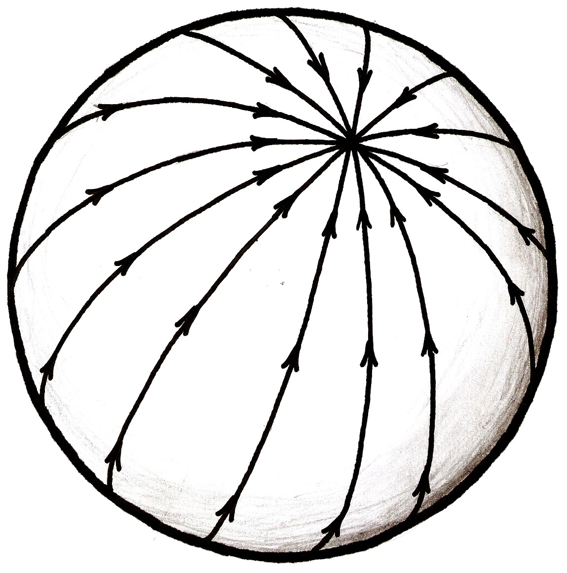
Figure 11: The conformal transformation of the celestial sphere corresponding to a boost towards the north pole: all points of the sphere are dragged along the arrows, towards the north pole. Equivalently, all points are dragged away from the south pole (which is not visible in this picture). In terms of stereographic coordinates obtained by projection through the south pole, this transformation corresponds to a contraction of the Riemann sphere, $z\mapsto e^{-\chi}z$ with $\chi>0$.

This result is somewhat counterintuitive, if we base our intuition on our habit of objects flowing past us when driving on the highway. Roughly speaking, one would expect that boosting in a given direction should make objects spread away from that direction. This intuition is well illustrated in the movie Star Wars Episode IV: A New Hope [48]. In the screenshot reproduced below, Han Solo and Chewbacca are sitting in the cockpit of the Millenium Falcon spaceship and have just switched on the “hyperspace” mode $-$ they are accelerating straight ahead. This acceleration corresponds to a continuous family of boosts in the direction of the acceleration. In the picture, these boosts are represented by stars flowing away from the direction of the motion, exactly as dictated by the naive, intuitive expectation just described:

Formula (4.9) tells us that this representation of the “jump to lightspeed” is wrong: what Han Solo and Chewbacca should really see is a contraction of the sphere at which they are looking, towards the direction of their acceleration. In other words, as long as the stars are far enough from the observer undergoing a boost, they should cluster close to the direction of the boost rather than flow away from it.

There is of course a subtlety in this argument: our intuition of objects flowing past us when we drive on the highway is obviously correct, so how come it contradicts the result (4.9)? The answer is that formula (4.9) holds only in the limit $r\rightarrow+\infty$, when the sphere we are talking about is located at an infinite distance from the observer. In that limit, the observer’s motion does not affect its distance to a point on the celestial sphere; in particular, all points on the sphere remain at an infinite distance from the observer, and there is no way they could flow past him. In real-world applications, however, all objects are necessarily located at some finite distance, in which case the corrections of order $1/r$ neglected in (4.8) become relevant. In particular, when Bob is moving with respect to Alice, the relation between his Bondi coordinates and those of Alice involves some time-dependent factors in the $1/r$ corrections. These corrections imply that the objects seen by Bob (be it stars, or cows on the side of the highway) do indeed flow past him when he gets close enough to them. In this sense the picture of the Millenium Falcon cockpit shown above is not completely wrong. Still, for stars located sufficiently far from Han Solo and Chewbacca, the $1/r$ corrections in (4.8) are negligible and the optical effect described by the contraction (4.9) is valid.

4.3.2 Subtleties

While $1/r$ corrections are the most obvious source of modifications to the result (4.9), there are several other caveats in trying to apply Lorentz transformations to realistic situations such as the jump to lightspeed in the Millenium Falcon. The first is the fact that the motion of the spaceship during the jump is actually accelerated, so that Han Solo and Chewbacca are definitely not inertial observers! This does not prevent us from guessing what should happen: roughly speaking, accelerated motion may be seen as an infinite sequence of infinitesimal boosts, so if (4.9) remains valid for each infinitesimal boost, one expects the celestial sphere seen by an accelerated observer to undergo a time-dependent contraction (in the direction of acceleration), with a scaling factor that gets smaller and smaller as time goes by. More precisely, since rapidity is the integral (1.23) of proper acceleration, the naive application of (4.9) to accelerated motion predicts that an accelerated observer, looking at the celestial sphere in the direction of his acceleration, should see a proper-time-dependent contraction with a scaling factor $\exp[-I(s)/c]$, where $I(s)$ is the integral (1.21) of proper acceleration over proper time.

The potential problem with this expectation is that special relativity was established for inertial observers from the very beginning, so one might fear that acceleration invalidates the application of special-relativistic techniques to the Millenium Falcon. Fortunately, there is in principle no obstacle in describing accelerated observers in special relativity [30]. For example, Thomas precession is a well known special-relativistic effect that applies to such observers [30, 49], and it is precisely derived by thinking of accelerated motion as a sequence of infinitesimal boosts. The only issue is that the reference frames associated with accelerated observers are not global coordinate systems $-$ they do not cover the whole of space-time. This is related to the existence of horizons: for instance, a uniformly accelerated observer in Minkowski space-time $-$ a Rindler observer $-$ cannot receive light rays coming from behind his future horizon [30]. Thus, since our definition of celestial spheres relied on the limit $r\rightarrow+\infty$ in Bondi coordinates, one may wonder whether acceleration invalidates our approach, as the limit may be ill-defined. We will not attempt to address this issue here, but we will rederive formula (4.9) in a local way at the end of this section. This will confirm that the optical effects of boosts on the celestial sphere do not actually rely on a large $r$ limit, as already mentioned at the end of subsection 4.1. In particular, the local nature of the derivation implies that it remains valid for an accelerated observer in the sense that acceleration deforms the shape of light-cones centered on the observer $-$ as is of course well-known in general relativity. Whether this deformation can be seen by an “asymptotic” computation analogous to the one explained above is another matter, which we will not discuss.

A second subtlety to be considered is the fact that the light seen by Han Solo and Chewbacca during the jump to lightspeed is blue-shifted due to the Doppler effect. As the velocity of the Millenium Falcon increases, the frequency of the light rays hitting the observers inside the cockpit increases as well. Eventually, the increase in frequency should become so high that the stars actually become invisible $-$ the starlight seen by the pilots of the spaceship has reached the ultraviolet region. Thus, the stars seen by Han Solo and Chewbacca not only move in the direction of acceleration, but they also change colour, becoming blue, then purple, then invisible.

This blue shift applies of course to any electromagnetic radiation reaching the observers inside the cockpit. In particular, it applies to the cosmic microwave background radiation. Thus, at sufficiently high velocities, the background radiation should reach the visible spectrum and the actual picture seen from the cockpit of the Millenium Falcon should include a fuzzy disc of light centered around the direction of the motion [50, 51]. Upon taking this effect into account and recalling that most stars become invisible because of the blue shift, one concludes that the actual landscape seen by Han Solo and his hairy companion is indeed far, far away from the image shown in the movie.

4.3.3 A local derivation

We have just seen that boosting an observer in a given direction affects his celestial sphere by contracting all points of the sphere towards that direction. Given the counterintuitive nature of this optical phenomenon, it is worthwile to rederive it using a different technique. Namely, consider two inertial observers, Alice and Bob, using inertial coordinates $(x^{\mu})$ and $(x^{\prime\mu})$ respectively. We take Bob’s coordinates to be boosted, with rapidity $\chi$, with respect to those of Alice. For definiteness, we will assume that the boost takes place along the $x^{1}$ direction, so that the relation between Bob’s coordinates and Alice’s coordinates is $x^{\prime\mu}={\Lambda^{\mu}}_{\nu}x^{\nu}$, with $\Lambda$ the matrix (1.19). Now suppose Alice and Bob both see one incoming photon, whose energy-momentum vector is $p=(E,-E\cos\theta,-E\sin\theta,0)$ in Alice’s coordinates, and $p^{\prime}=(E^{\prime},-E^{\prime}\cos\theta^{\prime},-E^{\prime}\sin\theta^{\prime},0)$ in Bob’s coordinates. (Here $E$ and $E^{\prime}$ are the photon’s energy in Alice’s and Bob’s frames, respectively.) The angle $\theta$ (resp. $\theta^{\prime}$) is the angle between the photon’s direction and the axis $x^{3}=x^{\prime 3}$ in Alice’s (resp. Bob’s) frame. The question is: what is the relation between $\theta^{\prime}$ and $\theta$?

Since 4-momentum transforms under boosts just as standard inertial coordinates do (the energy-momentum vector is a “four-vector”), we know that the photon’s 4-momentum in Bob’s and Alice’s coordinate systems are related by $p^{\prime}=\Lambda\cdot p$. Explicitly, this means that

$$\begin{pmatrix}E^{\prime}\\ -E^{\prime}\cos\theta^{\prime}\\ -E^{\prime}\sin\theta^{\prime}\\ 0\end{pmatrix}=\begin{pmatrix}\cosh\chi&-\sinh\chi&0&0\\ -\sinh\chi&\cosh\chi&0&0\\ 0&0&1&0\\ 0&0&0&1\end{pmatrix}\cdot\begin{pmatrix}E\\ -E\cos\theta\\ -E\sin\theta\\ 0\end{pmatrix}.$$

From this we read off $\tan\theta^{\prime}=\sin\theta/(\sinh\chi+\cosh\chi\,\cos\theta)$, which can be rewritten in terms of half angles as

$$\tan(\theta^{\prime}/2)-\frac{1}{\tan(\theta^{\prime}/2)}=e^{-\chi}\tan(\theta/2)-\frac{1}{e^{-\chi}\tan(\theta/2)}.$$

This is a quadratic equation for $\tan(\theta^{\prime}/2)$ as a function of $\tan(\theta/2)$. The solution that ensures $\theta^{\prime}=\theta$ when $\chi=0$ is the simplest one,

$$\tan(\theta^{\prime}/2)=e^{-\chi}\tan(\theta/2).$$ (4.10)

Since here $\theta$ and $\theta^{\prime}$ should be thought of as standard azimuthal coordinates on the sphere in unprimed and primed coordinate systems, we can relate them to the stereographic coordinate $z$ through relation (3.18). The result (4.10) thus coincides with the contraction (4.9), as it should. In particular, provided $\theta$ is in the first quadrant (between $0$ and $\pi/2$), $\theta^{\prime}$ is smaller than $\theta$ when the rapidity $\chi$ is positive. (Conversely, when $\theta$ is larger than $\pi/2$, then $\theta^{\prime}$ is larger than $\theta$, corresponding to the fact that points of the celestial sphere located in the direction opposite to the boost undergo a dilation.)

The important difference between this computation and the one based on Bondi coordinates is the fact that here we never needed to take a “large $r$” limit. The result (4.10) is valid locally, for any boosted observer detecting a light ray. This implies in particular that an accelerated observer looking in the direction of his/her acceleration should see a time-dependent contraction of the celestial sphere, just as mentioned above for the case of Han Solo and Chewbacca.

5 Conclusion

Let us take a look back at what we have done. We have seen how the Lorentz group arises as the set of homogeneous coordinate transformations between inertial observers in Minkowski space-time. Since it consists of linear transformations, it can be represented in terms of matrices. We have then shown that (the maximal connected subgroup of) this matrix group is isomorphic to $\mathrm{SL}(2,\mathbb{C})/\mathbb{Z}_{2}$ $-$ a type of relation that also occurs in other space-time dimensions. As observed in section 3, the group $\mathrm{SL}(2,\mathbb{C})/\mathbb{Z}_{2}$ also arises, somewhat coincidentally, as the group of conformal transformations of the sphere. The question, then, was whether there exists a relation between the action of Lorentz transformations on space-time and that of Möbius transformations on a sphere. We answered this question positively, by showing that the difference between the celestial spheres seen by two inertial observers whose coordinates are related by a Lorentz transformation is precisely a conformal transformation. Finally, we used this relation to discuss the slightly unexpected optical phenomenon associated with boosts: we saw that an observer boosted in a given direction sees the stars of his/her celestial sphere being dragged towards that direction. This result is applicable, in particular, to the jump to lightspeed as seen from the cockpit of the Millenium Falcon.

As emphasized in the introduction, the surprising aspect of the relation between Lorentz and conformal transformations is the fact that it links the action of a group on a four-dimensional space to its action on a two-dimensional manifold. Of course, from a mathematical viewpoint there is nothing wrong with that, but from an intuitive viewpoint it is not a priori obvious that such a connection has any physical meaning $-$ i.e. that this relation can actually be seen in a concrete experiment, such as accelerating in a spaceship. The purpose of these notes was to unveil that meaning, which is well known in the literature but perhaps less well known to undergraduate students following a course in special relativity, group theory, or even general relativity.

In fact, part of the motivation for these lectures was that the idea of relating some space to a lower-dimensional subspace is closely connected to certain recent developments in the study of (quantum) gravity, all encompassed under the general name of holography. Recall that a hologram is a two-dimensional surface that produces a three-dimensional image $-$ such an optical device is typically found on credit cards or banknotes. The idea of holography in quantum gravity [21, 22, 23, 24, 25] roughly states that there exists a correspondence (and in certain regimes an actual equivalence) between a gravitational system in $d$ space-time dimensions and some quantum theory living on a lower-dimensional subspace of the gravitational system $-$ one says that the two theories are “dual” to each other. In particular, according to this idea, the four-dimensional world that we see around us might be a “hologram” of some lower-dimensional theory. This correspondence is motivated by countless computations matching quantities evaluated on the high-dimensional, gravitational side, to some other quantities evaluated on the low-dimensional side; the interested reader may consult the abundant literature on the subject.

The modest result derived in these notes may be seen as a remnant of the holographic principle: we have shown that Lorentz invariance in four dimensions becomes conformal invariance in two dimensions upon focusing on celestial spheres. In fact, this feature is only part of a much larger construction, that is still under study today. Indeed, it was shown in the sixties by Bondi, van der Burg, Metzner and Sachs [13, 14] that the natural symmetry group of four-dimensional “asymptotically Minkowskian” space-times is an infinite-dimensional extension of the Poincaré group, known nowadays as the Bondi-Metzner-Sachs (BMS) group. The transformations of space-time generated by this group precisely act on “null infinity”, the region $r\rightarrow+\infty$ that we used in section 4 to define celestial spheres, and extend the natural action of Poincaré transformations on that region. In the holographic context, the BMS group is to be interpreted as the symmetry group of the would-be (as yet conjectural) dual field theory; the latter, if it exists, is expected to be some version of a conformal field theory (recall the brief discussion of subsection 3.4), since Lorentz transformations are part of the symmetry group and act as conformal transformations on celestial spheres. BMS symmetry has recently been the focus of renewed interest, as it was shown that it can be extended to include arbitrary, local conformal transformations of the celestial spheres [15, 16, 17], and also that it is related to standard quantum field theory in Minkowski space through certain “soft theorems” that were known in a completely different language ever since the sixties [52] (see e.g. [18, 19, 20], references therein, and their follow-ups). Many more open problems remain to be settled, both regarding holography in general, and BMS symmetry in particular; the hope of the author is that addressing such questions may open the door to a deeper understanding of quantum gravity.

References

References

- [1] J. Terrell, “Invisibility of the Lorentz Contraction,” Phys. Rev. 116 (Nov, 1959) 1041–1045.
- [2] R. Penrose, “The Apparent shape of a relativistically moving sphere,” Proc.Cambridge Phil.Soc. 55 (1959) 137–139.
- [3] R. Penrose and W. Rindler, Spinors and Space-Time: Volume 1, Two-Spinor Calculus and Relativistic Fields. Cambridge Monographs on Mathematical Physics. Cambridge University Press, 1987.
- [4] A. Held, E. T. Newman, and R. Posadas, “The Lorentz Group and the Sphere,” Journal of Mathematical Physics 11 (1970), no. 11, 3145–3154.
- [5] M. Henneaux, “Groupes et représentations: I. Groupe des rotations à 3 dimensions, groupe de Lorentz et groupe de Poincaré.” ULB, 2009. Available at http://www.ulb.ac.be/sciences/ptm/pmif/membres/notescours.html.
- [6] M. Henneaux, “Cours de relativité générale.” ULB, 2011.
- [7] J. Hladik and M. Chrysos, Introduction à la relativité restreinte: cours et exercices corrigés. Dunod, 2001.
- [8] J.-M. Lévy-Leblond, “One more derivation of the Lorentz transformation,” American Journal of Physics 44 (Mar., 1976) 271–277.
- [9] J.-M. Lévy-Leblond and J.-P. Provost, “Additivity, rapidity, relativity,” American Journal of Physics 47 (Dec., 1979) 1045–1049.
- [10] J.-M. Lévy-Leblond, “Speed(s),” American Journal of Physics 48 (May, 1980) 345–347.
- [11] P. Di Francesco, P. Mathieu, and D. Sénéchal, Conformal Field Theory. Springer, 1997.
- [12] R. Blumenhagen and E. Plauschinn, Introduction to Conformal Field Theory: With Applications to String Theory. Lecture notes in physics. Springer, 2009.
- [13] H. Bondi, M. G. J. van der Burg, and A. W. K. Metzner, “Gravitational waves in general relativity. vii. waves from axi-symmetric isolated systems,” Proceedings of the Royal Society of London A: Mathematical, Physical and Engineering Sciences 269 (1962), no. 1336, 21–52.
- [14] R. Sachs, “Asymptotic symmetries in gravitational theory,” Phys. Rev. 128 (Dec, 1962) 2851–2864.
- [15] G. Barnich and C. Troessaert, “Symmetries of asymptotically flat 4 dimensional spacetimes at null infinity revisited,” Phys.Rev.Lett. 105 (2010) 111103, 0909.2617.
- [16] G. Barnich and C. Troessaert, “Aspects of the BMS/CFT correspondence,” JHEP 1005 (2010) 062, 1001.1541.
- [17] T. Banks, “A Critique of pure string theory: Heterodox opinions of diverse dimensions,” hep-th/0306074. (see footnote 17).
- [18] A. Strominger, “On BMS Invariance of Gravitational Scattering,” JHEP 1407 (2014) 152, 1312.2229.
- [19] T. He, V. Lysov, P. Mitra, and A. Strominger, “BMS supertranslations and Weinberg’s soft graviton theorem,” 1401.7026.
- [20] D. Kapec, V. Lysov, S. Pasterski, and A. Strominger, “Semiclassical Virasoro symmetry of the quantum gravity -matrix,” JHEP 1408 (2014) 058, 1406.3312.
- [21] G. ’t Hooft, “Dimensional reduction in quantum gravity,” gr-qc/9310026.
- [22] L. Susskind, “The World as a hologram,” J.Math.Phys. 36 (1995) 6377–6396, hep-th/9409089.
- [23] J. M. Maldacena, “The Large N limit of superconformal field theories and supergravity,” Int.J.Theor.Phys. 38 (1999) 1113–1133, hep-th/9711200.
- [24] E. Witten, “Anti-de Sitter space and holography,” Adv.Theor.Math.Phys. 2 (1998) 253–291, hep-th/9802150.
- [25] S. Gubser, I. R. Klebanov, and A. M. Polyakov, “Gauge theory correlators from noncritical string theory,” Phys.Lett. B428 (1998) 105–114, hep-th/9802109.
- [26] A. Einstein, Relativity: the special and general theory. Henri Holt and Company, New York, 1920. Digital reprint available at http://www.ibiblio.org/ebooks/Einstein/Einstein_Relativity.pdf.
- [27] E. P. Wigner, “On Unitary Representations of the Inhomogeneous Lorentz Group,” Annals Math. 40 (1939) 149–204.
- [28] S. Weinberg, The Quantum Theory of Fields (Volume 1). Cambridge University Press, 1 ed., 1995.
- [29] F. Ferrari, “Cours de relativité générale.” ULB, 2010.
- [30] C. Misner, K. Thorne, and J. Wheeler, Gravitation. W. H. Freeman, 1973.
- [31] J. Cornwell, Group theory in physics. Techniques of physics. Academic Press, 1984.
- [32] B. Binegar, “Relativistic Field Theories in Three-Dimensions,” J.Math.Phys. 23 (1982) 1511.
- [33] D. Grigore, “The Projective unitary irreducible representations of the Poincare group in (1+2)-dimensions,” Journal of Mathematical Physics 34 (1993), no. 9, 4172–4189.
- [34] L. La Fuente-Gravy, “Le théorème de Hurwitz,” in Notes de la quatrième BSSM. Brussels, 2011. Available at https://bssm.ulb.ac.be/en/notes_2011.html.
- [35] T. Kugo and P. Townsend, “Supersymmetry and the division algebras,” Nuclear Physics B 221 (July, 1983) 357–380.
- [36] A. Sudbery, “Division algebras, (pseudo)orthogonal groups and spinors,” Journal of Physics A Mathematical General 17 (Apr., 1984) 939–955.
- [37] J. C. Baez, “The octonions,” Bull. Amer. Math. Soc 39 (2002) 145–205.
- [38] J. C. Baez and J. Huerta, “Division Algebras and Supersymmetry I,” 0909.0551.
- [39] J. C. Baez and J. Huerta, “Division Algebras and Supersymmetry II,” Adv.Theor.Math.Phys. 15 (2011) 1373–1410, 1003.3436.
- [40] J. Lee, Manifolds and Differential Geometry. Graduate studies in mathematics. American Mathematical Society, 2009.
- [41] F. Bourgeois, “Géométrie différentielle.” ULB, 2009. Available at http://homepages.ulb.ac.be/~nrichard/#MATH-F-310.
- [42] M. Bertelson, “Géométrie riemannienne.” ULB, 2011.
- [43] J. Brown and R. Churchill, Complex Variables and Applications. Brown-Churchill series. McGraw-Hill Higher Education, 2004.
- [44] M. Peskin and D. Schroeder, An Introduction to Quantum Field Theory. Advanced book classics. Addison-Wesley Publishing Company, 1995.
- [45] M. Duff, “Twenty years of the Weyl anomaly,” Class.Quant.Grav. 11 (1994) 1387–1404, hep-th/9308075.
- [46] A. A. Belavin, A. M. Polyakov, and A. B. Zamolodchikov, “Infinite conformal symmetry in two-dimensional quantum field theory,” Nuclear Physics B 241 (July, 1984) 333–380.
- [47] J. L. Cardy, “Operator Content of Two-Dimensional Conformally Invariant Theories,” Nucl.Phys. B270 (1986) 186–204.
- [48] “Star Wars Episode IV: A New Hope.” Dir. G. Lucas. Perf. M. Hamill, H. Ford, C. Fisher, P. Cushing, A. Guinness. 20th Century Fox, 1977.
- [49] W. Rindler, Relativity: Special, General, and Cosmological. Oxford University Press, 2001.
- [50] J. Argyle, R. Connors, K. Dexter, and C. Scoular, “P1_3 Relativistic Optics,” Journal of Physics Special Topics 11 (2012), no. 1,.
- [51] R. Connors, J. Argyle, K. Dexter, and C. Scoular, “P1_5 Relativistic Optics Strikes Back,” Journal of Physics Special Topics 11 (2012), no. 1,.
- [52] S. Weinberg, “Infrared photons and gravitons,” Phys.Rev. 140 (1965) B516–B524.