Four-loop Standard Model effective potential at leading order in QCD

Abstract

The leading QCD part of the four-loop contribution to the effective potential for the Standard Model Higgs field is found. As a byproduct, I also find the corresponding contribution to the four-loop beta function of the Higgs self-interaction coupling.

I Introduction

The effective potential Coleman:1973jx ; Jackiw:1974cv ; Sher:1988mj is an important tool for analyzing spontaneous symmetry breaking associated with scalar field vacuum expectation values (VEVs). In the Standard Model, it provides a quantitative link between the Lagrangian parameters and the VEV of the Higgs field. The fact that the Higgs boson mass is near 125 GeV implies that the electroweak vacuum is close to metastable, motivating a program of precise study of the stability criteria Sher:1988mj ; Lindner:1988ww ; Arnold:1991cv ; Ford:1992mv ; Casas:1994qy ; Espinosa:1995se ; Casas:1996aq ; Isidori:2001bm ; Espinosa:2007qp ; ArkaniHamed:2008ym ; Bezrukov:2009db ; Ellis:2009tp ; EliasMiro:2011aa ; Alekhin:2012py ; Bezrukov:2012sa ; Degrassi:2012ry ; Buttazzo:2013uya ; Jegerlehner:2013dpa ; Bednyakov:2013cpa . Of more general importance is the fact that the effective potential minimization condition allows one to determine and eliminate one of the Lagrangian parameters of the theory, typically the negative Higgs squared mass parameter, in favor of the radiatively corrected VEV.

The effective potential $V_{\rm eff}(\phi)$ can be obtained as the sum of one-particle irreducible vacuum Feynman graphs, computed in terms of particle masses and couplings that depend on a constant background scalar field $\phi$. In the normalization conventions of the present paper, the canonically normalized Standard Model Higgs complex doublet field $\Phi$ has a tree-level potential

$$V = m^{2}\Phi^{\dagger}\Phi+\lambda(\Phi^{\dagger}\Phi)^{2},$$ (1.1)

where $\lambda$ is the Higgs self-interaction coupling, and the negative Higgs squared mass parameter is $m^{2}$. The real neutral part of $\Phi$ is given by $(\phi+h)/\sqrt{2}$, where $\phi$ is the constant background field and $h$ is the physical Higgs real scalar boson field. The complete set of 1-loop and 2-loop contributions to the effective potential in Landau gauge are known for the Standard Model Ford:1992pn and for a general renormalizable field theory Martin:2001vx . Also known Martin:2013gka are the 3-loop contributions that only involve the strong coupling $g_{3}$ and the top-quark Yukawa coupling $y_{t}$. Contributions from Goldstone bosons can be resummed Martin:2014bca ; Elias-Miro:2014pca in order to avoid potential infrared singularities and spurious imaginary parts. The value of the background field at the minimum of the effective potential is the radiatively corrected VEV of the Higgs field.

The purpose of this paper is to extend the existing calculations of the effective potential $V_{\rm eff}(\phi)$ by obtaining the 4-loop contributions that are leading in the strong coupling $g_{3}$, using dimensional regularization Bollini:1972ui ; Ashmore:1972uj ; Cicuta:1972jf ; tHooft:1972fi ; tHooft:1973mm and the $\overline{\rm MS}$ renormalization scheme Bardeen:1978yd ; Braaten:1981dv . These contributions come from those diagrams that involve only quarks, gluons, and QCD ghost fields. I will work in the approximation that all quarks are massless except the top quark. This is an excellent approximation beyond 1-loop order, due to the small magnitudes of the Yukawa couplings of the bottom and other quarks. Then, in dimensional regularization, at least one top-quark loop must be present in a diagram in order for the contribution not to vanish. At loop order $\ell$, the resulting leading QCD contribution is proportional to $g_{3}^{2(\ell-1)}t^{2}$ multiplied by a polynomial of order $\ell$ in $\overline{\ln}(t)$, where

$$t \equiv y_{t}^{2}\phi^{2}/2,$$ (1.2)

is the field-dependent $\overline{\rm MS}$ top-quark squared mass, and

$$\overline{\ln}(t) \equiv \ln(t/Q^{2}),$$ (1.3)

where $Q$ is the $\overline{\rm MS}$ renormalization scale.

The organization of the remainder of this paper is as follows. In section II, I review the basis of scalar integrals used in the calculation. The effective potential in

$$d=4-2\epsilon,$$ (1.4)

spacetime dimensions is given in section III in terms of bare quantities and the basis integrals. In section IV, the bare parameters are re-expressed in terms of $\overline{\rm MS}$ quantities to obtain the effective potential in that renormalization scheme, after expanding in $\epsilon$. (This is more efficient than doing a separate calculation of counterterm diagrams.) In the process, I obtain the leading QCD contribution to the 4-loop beta function for $\lambda$, from the requirement that poles in $\epsilon$ do not appear in the effective potential when written in terms of the renormalized parameters. Some of the results, when given in general form in terms of group theory invariants, are rather lengthy and therefore are provided in ancillary electronic files rather than in print. Section V concludes with some brief comments on the numerical impact of the new results.

II Three-loop and four-loop integral basis

In the approximation of this paper, the only mass scale (other than the renormalization scale) is the top-quark mass. Therefore, it is convenient to write results in terms of Euclidean momentum integrals with each propagator having dimensionless mass 0 or 1. The dependence on the bare top-quark mass is then restored by dimensional analysis. Only integrals having an even number of massive propagators meeting at each vertex are needed in this paper. Momentum integrations in $d$ dimensions are normalized by

$$\int_{p} \equiv \int\frac{d^{d}p}{(2\pi)^{d}},$$ (2.1)

so that the 1-loop vacuum master integral is defined by

$$A \equiv \int_{p}\frac{1}{p^{2}+1}\>=\>\frac{\Gamma(1-d/2)}{(4\pi)^{d/2}}.$$ (2.2)

At 2-loop order, no new master integral appears. The necessary 3-loop and 4-loop integrals have been studied and used in refs. Broadhurst:1991fi ; Avdeev:1995eu ; Broadhurst:1998rz ; MATAD ; Laporta:2002pg ; Schroder:2002re ; Schroder:2005va ; Schroder:2005db ; Kniehl:2005yc ; Schroder:2005hy ; Chetyrkin:2006dh ; Chetyrkin:2006bj ; Boughezal:2006xk ; Bejdakic:2006vg ; Faisst:2006sr ; Bejdakic:2009zz ; Lee:2010hs ; Liu:2015fxa . Important applications include the calculations of the 4-loop QCD corrections Schroder:2005db ; Chetyrkin:2006bj ; Boughezal:2006xk to the $\rho$ parameter and decoupling rules for $\alpha_{S}$ and light quark masses across heavy quark thresholds Schroder:2005hy ; Liu:2015fxa . Figure 2.1 shows a basis for the master integrals needed Schroder:2002re for single-scale gauge theories at 3-loop order and 4-loop order. Each solid line represents a massive propagator denominator, and each dashed line represents a massless propagator denominator, and the Euclidean loop integrations are normalized according to eq. (2.1). So, for example,

$$I_{42} \equiv \int_{p}\int_{q}\int_{k}\frac{1}{p^{2}q^{2}(k^{2}+1)[(p+q+k)^{2}+1]}.$$ (2.3)

Also needed in the basis are products $A^{2}$, $A^{3}$, $A^{4}$, $AI_{40}$, and $AI_{42}$. All of the integrals used in this paper are reduced to the basis by repeated application of the integration by parts method IBP , using a strategy similar to that described in ref. Schroder:2002re .

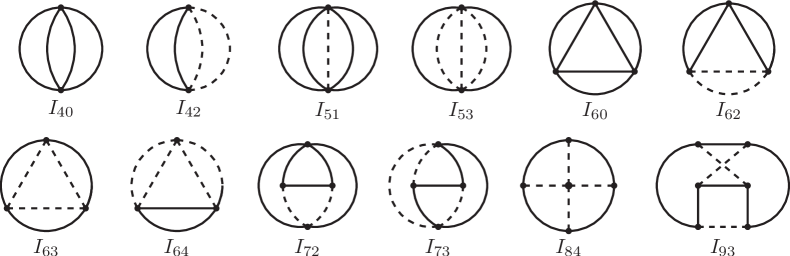
Figure 2.1: The 3-loop and 4-loop scalar basis integrals with one mass scale and an even number of massive propagators at each vertex. Massive propagator lines are solid, and massless propagator lines are dashed. The first subscript is the total number of propagators, and the second is the number of massless propagators.

The integrals $I_{42}$, $I_{53}$, and $I_{64}$ have non-zero masses confined to a single 1-loop self-energy subdiagram, and are therefore known analytically in terms of $\Gamma$ functions. In general, it is sufficient to have results for the basis integrals as expansions in $\epsilon$. However, with the basis chosen here, the coefficients of the basis integrals have poles in $1/\epsilon$ in addition to the poles inherent in the basis integrals. This means that it is necessary to have the expansions to certain positive powers of $\epsilon$ in most of the cases. The coefficients of expansions in $\epsilon$ of the other integrals have been given numerically with high precision and to sufficiently high order in $\epsilon$ in Schroder:2005va , using the Laporta difference equation method Laporta:2001dd . In principle this is enough for practical purposes, but it is nice to have analytical versions as well. These have been provided in refs. Schroder:2005va ; Bejdakic:2006vg ; Bejdakic:2009zz ; Lee:2010hs . Table 2.1 shows the order in $\epsilon$ to which each basis integral is needed in the present paper, as well as the highest order to which it is known analytically in terms of simple $\epsilon$-independent sums, and the source reference that provides that expansion.

Table 2.1: Summary of present analytical knowledge of 3-loop and 4-loop basis integrals needed in this paper and depicted in Figure 2.1. The second row shows the order in the expansion in $\epsilon$ needed here. The third row shows the highest order in the $\epsilon$ expansion to which the integral is presently known analytically in terms of simple $\epsilon$-independent sums, while the fourth row gives the source reference for that expansion. All integrals were also previously evaluated numerically to the necessary orders and beyond in ref. Schroder:2005va .

integral	$I_{40}$	$I_{42}$	$I_{51}$	$I_{53}$	$I_{60}$	$I_{62}$	$I_{63}$	$I_{64}$	$I_{72}$	$I_{73}$	$I_{84}$	$I_{93}$
needed	$\epsilon^{3}$	$\epsilon^{4}$	$\epsilon^{4}$	$\epsilon^{3}$	$\epsilon^{2}$	$\epsilon^{3}$	$\epsilon^{2}$	$\epsilon^{1}$	$\epsilon^{1}$	$\epsilon^{1}$	$\epsilon^{0}$	$\epsilon^{1}$
known	$\epsilon^{5}$	$\epsilon^{\infty}$	$\epsilon^{4}$	$\epsilon^{\infty}$	$\epsilon^{2}$	$\epsilon^{3}$	$\epsilon^{5}$	$\epsilon^{\infty}$	$\epsilon^{3}$	$\epsilon^{1}$	$\epsilon^{0}$	$\epsilon^{1}$
source	Bejdakic:2009zz	Schroder:2005va	Lee:2010hs	Schroder:2005va	Lee:2010hs	Bejdakic:2009zz	Bejdakic:2006vg	Schroder:2005va	Bejdakic:2009zz	Lee:2010hs	Lee:2010hs	Lee:2010hs

The (probably) transcendental numbers appearing in these coefficients up to the orders needed in this paper are $\pi$, $\ln(2)$, and

$$\zeta_{n} = \sum_{k=1}^{\infty}\frac{1}{k^{n}},$$ (2.4)

$$a_{n} = {\rm Li}_{n}(1/2)\>=\>\sum_{k=1}^{\infty}\frac{1}{2^{k}k^{n}},$$ (2.5)

$$s_{6} = \sum_{n=1}^{\infty}\sum_{k=1}^{n}\frac{(-1)^{n+k}}{n^{5}k},$$ (2.6)

although the last quantity cancels out of the results below. (The absence of this quantity could presumably have been made manifest by using the alternative basis of Chetyrkin:2006dh ; Faisst:2006sr .)

III Effective potential in terms of bare quantities

In this section, I find the 4-loop effective potential in terms of the bare quantities in $d=4-2\epsilon$ dimensions. These include the external scalar field $\phi_{B}$ and the bare Yukawa coupling $y_{tB}$ and QCD coupling $g_{3B}$. In the next section, the results will be converted to $\overline{\rm MS}$ parameters. The loop expansion for the effective potential is written as

$$V_{\rm eff}=\sum_{\ell=0}^{\infty}V^{(\ell)}_{B}.$$ (3.1)

The tree-level potential is

$$V^{(0)}_{B}=\frac{m^{2}_{B}}{2}\phi_{B}^{2}+\frac{\lambda_{B}}{4}\phi_{B}^{4},$$ (3.2)

where $\lambda_{B}$ and $m^{2}_{B}$ are the bare Higgs self-coupling and squared mass parameter, respectively. The latter will play no role in the following.

At each loop order, the contribution to the effective potential is given by the sum of 1-particle irreducible Feynman diagrams with no external legs and containing only quarks, gluons, and QCD ghosts. The pertinent contributions at loop order $\ell\geq 1$ are proportional to $g_{3B}^{2\ell-2}t_{B}^{2+\ell(d-4)/2}$, where

$$t_{B} = y_{tB}^{2}\phi_{B}^{2}/2$$ (3.3)

is the bare field-dependent top-quark mass. Results below will be given in terms of group theory invariants: the dimension of the fundamental representation $N_{c}$, the Casimir invariants of the adjoint and fundamental representations $C_{G}$ and $C_{F}$, the Dynkin index of the fundamental representation $T_{F}$, and the number of quark flavors $n_{q}$. In the Standard Model, these are given by

$$C_{G} = N_{c}=3,$$ (3.4)

$$C_{F} = \frac{N_{c}^{2}-1}{2N_{c}}=4/3,$$ (3.5)

$$T_{F} = 1/2,$$ (3.6)

$$n_{q} = 6,$$ (3.7)

but leaving them general provides more information for comparisons and checks. Diagrams at 2-loop order and higher are calculated with a gluon propagator

$$-i[g^{\mu\nu}/p^{2}-(1-\xi)p^{\mu}p^{\nu}/(p^{2})^{2}],$$ (3.8)

where $\xi=1$ for Feynman gauge and $\xi=0$ for Landau gauge. The dependence on the (bare) QCD gauge-fixing parameter $\xi$ cancels at the level of the basis integrals, providing a stringent check.

The contributions involving only quarks, gluons, and QCD ghosts, up to 3-loop order, are Martin:2013gka :

$$V^{(1)}_{B} = -4N_{c}t_{B}^{d/2}A/d,$$ (3.9)

$$V^{(2)}_{B} = N_{c}C_{F}g_{3B}^{2}t_{B}^{d-2}A^{2}{(d-1)(d-2)}/{(d-3)},$$ (3.10)

$$V^{(3)}_{B} = g_{3B}^{4}t^{3d/2-4}N_{c}C_{F}\Bigl{\{}C_{G}\Bigl{[}\frac{(2-d)^{3}}{2(d-4)^{2}(d-3)}A^{3}+\frac{(3-d)(d^{3}-13d^{2}+50d-48)}{4(d-4)^{2}}I_{40}$$ (3.11)

$$+\frac{(d-2)^{2}(2d^{2}-17d+32)}{2(d-4)(2d-7)}I_{42}\Bigr{]}+C_{F}\Bigl{[}\frac{(d-6)(d-3)(d^{2}-7d+8)}{2(d-4)^{2}}I_{40}$$

$$+\frac{(d-2)^{2}(-d^{5}+13d^{4}-67d^{3}+181d^{2}-274d+188)}{2(d-4)^{2}(d-3)^{2}}A^{3}$$

$$+\frac{(2-d)(2d^{3}-21d^{2}+67d-68)}{(d-4)(d-3)}I_{42}\Bigr{]}+T_{F}\Bigl{[}\frac{2(5-d)(d-2)^{3}}{(d-6)(d-4)(d-3)}A^{3}$$

$$+\frac{d^{3}-7d^{2}+6d+16}{(d-6)(4-d)}I_{40}+(n_{q}-1)\frac{4(d-3)(d-2)}{7-2d}I_{42}\Bigr{]}\Bigr{\}}.$$

For the 4-loop order contributions involving quarks, gluons, and QCD ghosts, there are 51 Feynman diagrams, which are reduced to linear combinations of the 13 integrals from the set

$${\cal I}=\{A^{4},\>AI_{40},\>AI_{42},\>I_{51},\>I_{53},\>I_{60},\>I_{62},\>I_{63},\>I_{64},\>I_{72},\>I_{73},\>I_{84},\>I_{93}\},$$ (3.12)

using integration by parts identities. The four-loop effective potential contribution is then organized in terms of the group theory invariants from the set

$${\cal{G}}=\{C_{G}^{2},\>C_{G}T_{F},\>C_{G}T_{F}n_{q},\>C_{G}C_{F},\>C_{F}^{2},\>C_{F}T_{F},\>C_{F}T_{F}n_{q},\>T_{F}^{2},\>T_{F}^{2}n_{q},\>T_{F}^{2}n_{q}^{2}\},$$ (3.13)

so that the result is written as:

$$V_{B}^{(4)}=g_{3B}^{6}t_{B}^{2d-6}C_{F}N_{c}\sum_{\cal{G}}\sum_{{\cal I}}\,{\cal{G}}\,{\cal I}\,V^{(4)}_{B}({\cal{G}},{\cal{I}}).$$ (3.14)

The 130 coefficients $V^{(4)}_{B}({\cal{G}},{\cal{I}})$ are rational functions of the spacetime dimension $d$. Although 58 of them vanish, this list of coefficients is still rather lengthy, so they are not shown in print here. Instead, they are provided in an ancillary electronic file called V4bare.txt included with the arXiv submission for this article.

IV Effective potential in terms of renormalized quantities

In this section, I obtain the effective potential in the $\overline{\rm MS}$ renormalization scheme by translating the bare quantities into $\overline{\rm MS}$ quantities. Because $\int d^{d}xV$ must be dimensionless in order to be exponentiated in the path integral, one must introduce an arbitrary regularization scale $\mu$, which is related to the $\overline{\rm MS}$ renormalization scale $Q$ by Bardeen:1978yd ; Braaten:1981dv :

$$Q^{2}=4\pi e^{-\gamma_{E}}\mu^{2}.$$ (4.1)

Then, in the $\overline{\rm MS}$ scheme, one writes:

$$\phi_{B} = \mu^{-\epsilon}\phi\sqrt{Z_{\phi}},$$ (4.2)

$$Z_{\phi} = 1+\sum_{\ell=1}^{\infty}\sum_{n=1}^{\ell}\frac{z^{\phi}_{\ell,n}}{(16\pi^{2})^{\ell}\epsilon^{n}},$$ (4.3)

$$x_{kB} = \mu^{\rho_{x_{k}}\epsilon}\Bigl{(}x_{k}+\sum_{\ell=1}^{\infty}\sum_{n=1}^{\ell}\frac{z^{x_{k}}_{\ell,n}}{(16\pi^{2})^{\ell}\epsilon^{n}}\Bigr{)}.$$ (4.4)

The subscript $B$ labels bare quantities, while the absence of a subscript $B$ indicates the corresponding $\overline{\rm MS}$ renormalized quantity. The exponent $\ell$ is the loop order, while $k$ is an index that runs over the list of Lagrangian parameters, including $x_{k}=\lambda,y_{t},g_{3}$. The mass dimensions of the bare parameters determine that $\rho_{\lambda}=2$ and $\rho_{g_{3}}=\rho_{y_{t}}=1$, in order that the renormalized couplings $\lambda,g_{3}$, and $y_{t}$ are dimensionless and $\phi$ has mass dimension 1. The counter-term quantities $z^{\phi}_{\ell,n}$ and $z^{x_{k}}_{\ell,n}$ are polynomials in the $\overline{\rm MS}$ renormalized parameters $x_{j}$, and do not depend on $\epsilon$ or $\phi$. They are determined by the requirement that the full effective potential (and all physical observables) are free of ultraviolet poles in $\epsilon$ when expressed in terms of the $\overline{\rm MS}$ quantities.

The anomalous dimension for $\phi$ and the $\overline{\rm MS}$ beta functions for the parameters $x_{k}$ are defined by

$$\gamma \equiv -Q\frac{d\ln\phi}{dQ}\Bigl{|}_{\epsilon=0}\>=\>-Q\frac{d\ln\phi}{dQ}+\epsilon\>=\>\frac{1}{2}Q\frac{d}{dQ}\ln(Z_{\phi}),$$ (4.5)

$$\beta_{x_{k}} \equiv Q\frac{dx_{k}}{dQ}\Bigl{|}_{\epsilon=0}\>=\>Q\frac{dx_{k}}{dQ}+\epsilon\rho_{x_{k}}x_{k}.$$ (4.6)

Because the bare quantities $\phi_{B}$ and $x_{kB}$ do not depend on $Q$, the anomalous dimension and beta functions are determined by the simple pole counterterms, so that:

$$\gamma = \sum_{\ell=1}^{\infty}\frac{1}{(16\pi^{2})^{\ell}}\gamma^{(\ell)},$$ (4.7)

$$\beta_{x_{k}} = \sum_{\ell=1}^{\infty}\frac{1}{(16\pi^{2})^{\ell}}\beta_{x_{k}}^{(\ell)},$$ (4.8)

where the $\ell$-loop contributions are:

$$\gamma^{(\ell)} = -\ell z^{\phi}_{\ell,1},$$ (4.9)

$$\beta_{x_{k}}^{(\ell)} = 2\ell z^{x_{k}}_{\ell,1}.$$ (4.10)

The higher pole counterterms are also fixed by consistency conditions

$$\ell z^{\phi}_{\ell,n} = \sum_{\ell^{\prime}=1}^{\ell-n+1}\Bigl{(}-\gamma^{(\ell^{\prime})}+\frac{1}{2}\sum_{j}\beta_{x_{j}}^{(\ell^{\prime})}\frac{\partial}{\partial x_{j}}\Bigr{)}z^{\phi}_{\ell-\ell^{\prime},n-1},$$ (4.11)

$$2\ell z^{x_{k}}_{\ell,n} = \sum_{\ell^{\prime}=1}^{\ell-n+1}\sum_{j}\beta_{x_{j}}^{(\ell^{\prime})}\frac{\partial}{\partial x_{j}}z^{x_{k}}_{\ell-\ell^{\prime},n-1}.$$ (4.12)

for $\ell\geq n\geq 2$.

The coefficients $z^{\phi}_{\ell,n}$ and $z^{x_{k}}_{\ell,n}$ for $\ell\leq 3$ are thus determined by the known results for the Standard Model beta functions and Higgs scalar anomalous dimension given in MVI ; MVII ; Jack:1984vj ; MVIII ; Chetyrkin:2012rz ; Chetyrkin:2013wya ; Bednyakov:2013eba . (Extensions to QCD 4-loop and 5-loop order can be found in vanRitbergen:1997va ; Czakon:2004bu ; Chetyrkin:1997dh ; Vermaseren:1997fq ; Baikov:2014qja ; Marquard:2015qpa .) Keeping only the contributions needed for the approximation of the present paper, they are:

$$z^{\lambda}_{1,1} = -N_{c}y_{t}^{4}+\ldots,$$ (4.13)

$$z^{\lambda}_{2,1} = g_{3}^{2}y_{t}^{4}(-2N_{c}C_{F})+\ldots,$$ (4.14)

$$z^{\lambda}_{2,2} = g_{3}^{2}y_{t}^{4}(6N_{c}C_{F})+\ldots,$$ (4.15)

$$z^{\lambda}_{3,1} = g_{3}^{4}y_{t}^{4}N_{c}C_{F}\left[\left(8\zeta_{3}-\frac{109}{6}\right)C_{G}+\left(\frac{131}{6}-16\zeta_{3}\right)C_{F}+\left(16+\frac{10}{3}n_{q}\right)T_{F}\right]+\ldots,$$ (4.16)

$$z^{\lambda}_{3,2} = g_{3}^{4}y_{t}^{4}N_{c}C_{F}\left(24C_{G}+10C_{F}-16T_{F}n_{q}/3\right)+\ldots,$$ (4.17)

$$z^{\lambda}_{3,3} = g_{3}^{4}y_{t}^{4}N_{c}C_{F}\left(-22C_{G}/3-24C_{F}+8T_{F}n_{q}/3\right)+\ldots,$$ (4.18)

$$z^{y_{t}}_{1,1} = g_{3}^{2}y_{t}(-3C_{F})+\ldots,$$ (4.19)

$$z^{y_{t}}_{2,1} = g_{3}^{4}y_{t}C_{F}\Bigl{(}-\frac{97}{12}C_{G}-\frac{3}{4}C_{F}+\frac{5}{3}T_{F}n_{q}\Bigr{)}+\ldots,\phantom{xxx}$$ (4.20)

$$z^{y_{t}}_{2,2} = g_{3}^{4}y_{t}C_{F}\Bigl{(}\frac{11}{2}C_{G}+\frac{9}{2}C_{F}-2T_{F}n_{q}\Bigr{)}+\ldots,$$ (4.21)

$$z^{y_{t}}_{3,1} = g_{3}^{6}y_{t}C_{F}\biggl{[}-\frac{11413}{324}C_{G}^{2}+\frac{43}{4}C_{G}C_{F}-\frac{43}{2}C_{F}^{2}+\left(\frac{556}{81}+16\zeta_{3}\right)C_{G}T_{F}n_{q}$$ (4.22)

$$+\left(\frac{46}{3}-16\zeta_{3}\right)C_{F}T_{F}n_{q}+\frac{140}{81}T_{F}^{2}n_{q}^{2}\biggr{)}+\ldots,$$

$$z^{y_{t}}_{3,2} = g_{3}^{6}y_{t}C_{F}\Bigl{(}\frac{1679}{54}C_{G}^{2}+\frac{313}{12}C_{F}C_{G}+\frac{9}{4}C_{F}^{2}-\frac{484}{27}C_{G}T_{F}n_{q}$$ (4.23)

$$-\frac{29}{3}C_{F}T_{F}n_{q}+\frac{40}{27}T_{F}^{2}n_{q}^{2}\Bigr{)}+\ldots,$$

$$z^{y_{t}}_{3,3} = g_{3}^{6}y_{t}C_{F}\Bigl{(}-\frac{121}{9}C_{G}^{2}+\frac{88}{9}C_{G}T_{F}n_{q}-\frac{33}{2}C_{G}C_{F}-\frac{9}{2}C_{F}^{2}+6C_{F}T_{F}n_{q}-\frac{16}{9}T_{F}^{2}n_{q}^{2}\Bigr{)}+\ldots,\phantom{xxxx}$$ (4.24)

$$z^{g_{3}}_{1,1} = g_{3}^{3}\Bigl{(}-\frac{11}{6}C_{G}+\frac{2}{3}T_{F}n_{q}\Bigr{)},$$ (4.25)

$$z^{g_{3}}_{2,1} = g_{3}^{5}\Bigl{(}-\frac{17}{6}C_{G}^{2}+\frac{5}{3}C_{G}T_{F}n_{q}+C_{F}T_{F}n_{q}\Bigr{)}+\ldots,$$ (4.26)

$$z^{g_{3}}_{2,2} = g_{3}^{5}\Bigl{(}\frac{121}{24}C_{G}^{2}-\frac{11}{3}C_{G}T_{F}n_{q}+\frac{2}{3}T_{F}^{2}n_{q}^{2}\Bigr{)}+\ldots,$$ (4.27)

while the $z^{\phi}_{\ell,n}$ do not contribute at all at leading order in QCD. Now, expanding eq. (3.1) with eqs. (3.2), (3.9), (3.10), (3.11), and (3.14) to order $1/\epsilon$, and requiring the 4-loop simple pole terms to cancel, I find:

$$z^{\lambda}_{4,1} = y_{t}^{4}g_{3}^{6}N_{c}C_{F}\Biggl{[}C_{G}^{2}\left(\frac{470}{3}\zeta_{3}-130\zeta_{5}-\frac{121547}{972}-\frac{11\pi^{4}}{45}\right)+C_{G}T_{F}\left(\frac{1472}{9}+88\zeta_{3}-40\zeta_{5}\right)$$ (4.28)

$$+C_{G}T_{F}n_{q}\left(4\zeta_{3}-\frac{661}{243}+\frac{16\pi^{4}}{45}\right)+C_{G}C_{F}\left(\frac{896}{3}-\frac{826}{3}\zeta_{3}+180\zeta_{5}+\frac{4\pi^{4}}{45}\right)$$

$$+C_{F}^{2}\left(12\zeta_{3}+40\zeta_{5}-\frac{1471}{6}+\frac{4\pi^{4}}{5}\right)-16C_{F}T_{F}+C_{F}T_{F}n_{q}\left(\frac{281}{6}+\frac{8}{3}\zeta_{3}-\frac{4\pi^{4}}{9}\right)$$

$$-T_{F}^{2}n_{q}\frac{64}{9}+T_{F}^{2}n_{q}^{2}\left(\frac{2728}{243}-\frac{32}{3}\zeta_{3}\right)\Biggr{]}+\ldots,$$

$$z^{\lambda}_{4,2} = y_{t}^{4}g_{3}^{6}N_{c}C_{F}\biggl{[}\left(\frac{7811}{54}-\frac{44\zeta_{3}}{3}\right)C_{G}^{2}-\frac{88}{3}C_{G}T_{F}+\left(-\frac{128\zeta_{3}}{3}-\frac{1138}{27}\right)C_{G}T_{F}n_{q}$$ (4.29)

$$+\left(\frac{131}{9}+\frac{16}{3}\zeta_{3}\right)C_{G}C_{F}+\left(2+48\zeta_{3}\right)C_{F}^{2}-48C_{F}T_{F}$$

$$+\left(-\frac{451}{9}+\frac{112}{3}\zeta_{3}\right)C_{F}T_{F}n_{q}+\frac{32}{3}T_{F}^{2}n_{q}-\frac{80}{27}T_{F}^{2}n_{q}^{2}\biggr{]}+\ldots,$$

$$z^{\lambda}_{4,3} = y_{t}^{4}g_{3}^{6}N_{c}C_{F}\biggl{[}-61C_{G}^{2}+\frac{322}{9}C_{G}T_{F}n_{q}-\frac{562}{3}C_{G}C_{F}-39C_{F}^{2}+\frac{146}{3}C_{F}T_{F}n_{q}$$ (4.30)

$$-\frac{32}{9}T_{F}^{2}n_{q}^{2}\biggr{]}+\ldots,$$

$$z^{\lambda}_{4,4} = y_{t}^{4}g_{3}^{6}N_{c}C_{F}\biggl{[}\frac{121}{9}C_{G}^{2}-\frac{88}{9}C_{G}T_{F}n_{q}+66C_{G}C_{F}+72C_{F}^{2}-24C_{F}T_{F}n_{q}$$ (4.31)

$$+\frac{16}{9}T_{F}^{2}n_{q}^{2}\biggr{]}+\ldots,$$

where the ellipses refer to contributions that are lower order in $g_{3}$. From eqs (4.10) and (4.28), I find the leading QCD 4-loop contribution to $\beta_{\lambda}$:

$$\beta^{(4)}_{\lambda} = y_{t}^{4}g_{3}^{6}N_{c}C_{F}\Biggl{[}C_{G}^{2}\left(\frac{3760}{3}\zeta_{3}-1040\zeta_{5}-\frac{243094}{243}-\frac{88\pi^{4}}{45}\right)+C_{G}T_{F}\left(\frac{11776}{9}+704\zeta_{3}-320\zeta_{5}\right)$$ (4.32)

$$+C_{G}T_{F}n_{q}\left(32\zeta_{3}-\frac{5288}{243}+\frac{128\pi^{4}}{45}\right)+C_{G}C_{F}\left(\frac{7168}{3}-\frac{6608}{3}\zeta_{3}+1440\zeta_{5}+\frac{32\pi^{4}}{45}\right)$$

$$+C_{F}^{2}\left(96\zeta_{3}+320\zeta_{5}-\frac{5884}{3}+\frac{32\pi^{4}}{5}\right)-128C_{F}T_{F}+C_{F}T_{F}n_{q}\left(\frac{1124}{3}+\frac{64}{3}\zeta_{3}-\frac{32\pi^{4}}{9}\right)$$

$$-T_{F}^{2}n_{q}\frac{512}{9}+T_{F}^{2}n_{q}^{2}\left(\frac{21824}{243}-\frac{256}{3}\zeta_{3}\right)\Biggr{]}+\ldots.$$

Now taking the limit $\epsilon\rightarrow 0$, the effective potential is obtained in a loop expansion as

$$V_{\rm eff}=\sum_{\ell=0}^{\infty}\frac{1}{(16\pi^{2})^{\ell}}V^{(\ell)}.$$ (4.33)

Note that unlike the loop expansion with bare parameters, eq. (3.1), here loop factors $1/(16\pi^{2})^{\ell}$ have been extracted, similarly to eqs. (4.7) and (4.8). In terms of $t$ and $\overline{\ln}(t)$ defined in eqs. (1.2) and (1.3), the previously known results for the leading QCD effective potential contributions are:

$$V^{(0)} = \frac{m^{2}}{2}\phi^{2}+\frac{\lambda}{4}\phi^{4},$$ (4.34)

$$V^{(1)} = -N_{c}t^{2}\bigl{[}\overline{\ln}(t)-3/2\bigr{]},$$ (4.35)

$$V^{(2)} = g_{3}^{2}N_{c}C_{F}t^{2}\bigl{[}6\overline{\ln}^{2}(t)-16\overline{\ln}(t)+18\bigr{]},\phantom{xxx}$$ (4.36)

from ref. Ford:1992pn , and the three-loop result Martin:2013gka :

$$V^{(3)} = g_{3}^{4}N_{c}C_{F}t^{2}\Bigl{\{}C_{G}\Bigr{[}-\frac{22}{3}\overline{\ln}^{3}(t)+\frac{185}{3}\overline{\ln}^{2}(t)+(24\zeta_{3}-\frac{1111}{6})\overline{\ln}(t)$$ (4.37)

$$+\frac{2609}{12}+\frac{44}{45}\pi^{4}-\frac{232}{3}\zeta_{3}+\frac{16}{3}\ln^{2}(2)[\pi^{2}-\ln^{2}(2)]-128a_{4}\Bigl{]}$$

$$+C_{F}\Bigr{[}-24\overline{\ln}^{3}(t)+63\overline{\ln}^{2}(t)-(48\zeta_{3}+\frac{121}{2})\overline{\ln}(t)+\frac{85}{12}-\frac{88}{45}\pi^{4}$$

$$+192\zeta_{3}-\frac{32}{3}\ln^{2}(2)[\pi^{2}-\ln^{2}(2)]+256a_{4}\Bigl{]}+T_{F}\Bigr{[}48\overline{\ln}(t)-\frac{232}{3}+96\zeta_{3}\Bigl{]}$$

$$+T_{F}n_{q}\Bigr{[}\frac{8}{3}\overline{\ln}^{3}(t)-\frac{52}{3}\overline{\ln}^{2}(t)+\frac{142}{3}\overline{\ln}(t)-\frac{161}{3}-\frac{64}{3}\zeta_{3}\Bigl{]}\Bigr{\}}.$$

The new 4-loop result (with group-theory quantities left general) takes the form:

$$V^{(4)}=g_{3}^{6}C_{F}N_{c}t^{2}\sum_{\cal{G}}\sum_{n=0}^{4}\,{\cal{G}}\,\overline{\ln}^{n}(t)\,V^{(4)}({\cal{G}},n),$$ (4.38)

in terms of the group theory invariants in the set ${\cal G}$ from eq. (3.13). The list of 50 coefficients $V^{(4)}({\cal{G}},n)$ is again rather lengthy, and so is provided in another ancillary electronic file V4MSbar.txt. After substituting in the Standard Model values for the group theory constants, the result combines and simplifies to:

$$V^{(4)} = g_{3}^{6}t^{2}\Biggl{[}\frac{13820381}{270}+\frac{1747112\zeta_{3}}{45}+\frac{1984\zeta_{5}}{9}-\frac{40288\zeta_{3}^{2}}{9}-\frac{298894\pi^{4}}{1215}-\frac{1780\pi^{6}}{243}+\frac{5888\ln^{5}(2)}{135}$$ (4.39)

$$-\frac{5888}{81}\pi^{2}\ln^{3}(2)-\frac{36064}{405}\pi^{4}\ln(2)+\frac{78464}{81}\ln^{2}(2)[\ln^{2}(2)-\pi^{2}]+\frac{627712a_{4}}{27}-\frac{47104a_{5}}{9}$$

$$+\overline{\ln}(t)\left(\frac{27680\zeta_{3}}{3}-\frac{63200\zeta_{5}}{9}-\frac{1547146}{27}-\frac{208\pi^{4}}{9}+\frac{640}{3}\ln^{2}(2)[\ln^{2}(2)-\pi^{2}]+5120a_{4}\right)$$

$$+(30584-2400\zeta_{3})\overline{\ln}^{2}(t)-9144\overline{\ln}^{3}(t)+1380\overline{\ln}^{4}(t)\Biggr{]}.$$

Equation (4.39) can be consistently added to the 3-loop effective potential as given in refs. Ford:1992pn and Martin:2013gka . Also, the condition for the minimum $v=\phi_{\rm min}$ of the Landau gauge effective potential of the Standard Model (including the effects of resummation of the Goldstone boson contributions from the terms up to 3-loop order) is obtained by subtracting

$$\frac{1}{(16\pi^{2})^{4}}\widehat{\Delta}_{4} = \frac{1}{(16\pi^{2})^{4}}\frac{1}{v}\left.\frac{\partial V^{(4)}}{\partial\phi}\right|_{\phi=v}$$ (4.40)

computed using eq. (1.2) and (1.3) above, from the right-hand side of eq. (4.18) of ref. Martin:2014bca .

V Discussion

The main results of this paper are the leading QCD 4-loop contributions to the Higgs self-coupling beta function $\beta_{\lambda}$ and to the effective potential and its minimization condition. In each case, it is certainly possible that other contributions at 4-loop order, and the presently unknown 3-loop effects involving electroweak couplings in the case of the effective potential, could be numerically comparable to or even larger than the ones found here. The same is certainly true of parametric uncertainties from the top-quark Yukawa coupling (or mass) and the strong coupling. Therefore the results found here are perhaps most useful, for the present, as ways of formalizing estimates of purely theoretical error.

The 4-loop leading QCD contribution of eq. (4.32) to the $\lambda$ beta function can be expressed in numerical form as

$$\Delta\beta_{\lambda} = \,\frac{1}{(16\pi^{2})^{4}}\>8308.17g_{3}^{6}y_{t}^{4}.$$ (5.1)

This can be compared to the leading QCD 1, 2, and 3-loop contributions:

$$\beta^{\rm{leading~{}QCD}}_{\lambda} = \frac{1}{16\pi^{2}}(-6y_{t}^{4})+\frac{1}{(16\pi^{2})^{2}}(-32g_{3}^{2}y_{t}^{4})+\frac{1}{(16\pi^{2})^{3}}(-100.402g_{3}^{4}y_{t}^{4}).$$ (5.2)

We see that the 4-loop contribution has a sign opposite to that of the other terms, and is larger in magnitude than one might have expected from a simple geometric progression. However, its magnitude is still only half as big as the 3-loop term in eq. (5.2) even at $Q=M_{t}$, and in absolute terms it makes only a tiny difference in extrapolating $\lambda$ to high energy scales.

The effective potential contribution of eq. (4.39) can similarly be expressed in numerical form as:

$$V^{(4)} = g_{3}^{6}t^{2}\Bigl{[}59366.97-54056.36\,\overline{\ln}(t)+27699.06\,\overline{\ln}^{2}(t)-9144\,\overline{\ln}^{3}(t)+1380\,\overline{\ln}^{4}(t)\Bigr{]}.$$ (5.3)

It follows that the corresponding contribution to the effective potential minimization condition

$$m^{2}+\lambda v^{2} = -\frac{1}{16\pi^{2}}\widehat{\Delta}_{1}-\frac{1}{(16\pi^{2})^{2}}\widehat{\Delta}_{2}-\frac{1}{(16\pi^{2})^{3}}\widehat{\Delta}_{3}-\frac{1}{(16\pi^{2})^{4}}\widehat{\Delta}_{4}+\ldots$$ (5.4)

is, numerically:

$$\widehat{\Delta}_{4} = g_{3}^{6}y_{t}^{2}t\left[64677.58-52714.59\,\overline{\ln}(t)+27966.13\,\overline{\ln}^{2}(t)-12768\,\overline{\ln}^{3}(t)+2760\,\overline{\ln}^{4}(t)\right],$$ (5.5)

where $\widehat{\Delta}_{\ell}$ for $\ell=1,2,3$ were given in ref. Martin:2014bca . Consider the VEV and other $\overline{\rm MS}$ parameters of the Standard Model at benchmark values

$$v(M_{t}) = \mbox{246.647 GeV},$$ (5.6)

$$\lambda(M_{t}) = 0.12597,$$ (5.7)

$$y_{t}(M_{t}) = 0.93690,$$ (5.8)

$$g_{3}(M_{t}) = 1.1666,$$ (5.9)

$$g(M_{t}) = 0.647550,$$ (5.10)

$$g^{\prime}(M_{t}) = 0.358521,$$ (5.11)

at $Q=M_{t}=173.34$ GeV. These choices provide agreement with the measured values of the $h$, $W$, and $Z$ boson masses in the pure $\overline{\rm MS}$ scheme Martin:2014cxa ; Martin:2015lxa ; Martin:2015rea . Using only the previously known 3-loop contributions in eq. (5.4), the resulting Higgs squared mass parameter is: $m^{2}(M_{t})=-(92.890\>{\rm GeV})^{2}$. Now including the new contribution of eq. (5.5) gives instead $m^{2}(M_{t})=-(92.926\>{\rm GeV})^{2}$. Thus I find

$$\Delta\left(\sqrt{-m^{2}}\right) = 36\>{\rm MeV}$$ (5.12)

from the leading QCD 4-loop contribution, at the scale $Q=M_{t}$. The parameter $m^{2}$ is not directly constrained by experiment, but it can be connected to ultraviolet completions that may predict it in terms of other underlying parameters that can be measured, eventually. This could occur in models of supersymmetry breaking, for example.

Acknowledgments: This work was supported in part by the National Science Foundation grant number PHY-1417028.

References

• (1) S. R. Coleman and E. J. Weinberg, “Radiative Corrections as the Origin of Spontaneous Symmetry Breaking,” Phys. Rev. D 7, 1888 (1973).
• (2) R. Jackiw, “Functional evaluation of the effective potential,” Phys. Rev. D 9, 1686 (1974).
• (3) M. Sher, “Electroweak Higgs Potentials and Vacuum Stability,” Phys. Rept.  179, 273 (1989), and references therein.
• (4) M. Lindner, M. Sher and H. W. Zaglauer, “Probing Vacuum Stability Bounds at the Fermilab Collider,” Phys. Lett. B 228, 139 (1989).
• (5) P. B. Arnold and S. Vokos, “Instability of hot electroweak theory: bounds on m(H) and M(t),” Phys. Rev. D 44, 3620 (1991).
• (6) C. Ford, D. R. T. Jones, P. W. Stephenson and M. B. Einhorn, “The Effective potential and the renormalization group,” Nucl. Phys. B 395, 17 (1993) [hep-lat/9210033].
• (7) J. A. Casas, J. R. Espinosa and M. Quirós, “Improved Higgs mass stability bound in the standard model and implications for supersymmetry,” Phys. Lett. B 342, 171 (1995) [hep-ph/9409458].
• (8) J. R. Espinosa and M. Quiros, “Improved metastability bounds on the standard model Higgs mass,” Phys. Lett. B 353, 257 (1995) [hep-ph/9504241].
• (9) J. A. Casas, J. R. Espinosa and M. Quiros, “Standard model stability bounds for new physics within LHC reach,” Phys. Lett. B 382 (1996) 374 [hep-ph/9603227].
• (10) G. Isidori, G. Ridolfi and A. Strumia, “On the metastability of the standard model vacuum,” Nucl. Phys. B 609, 387 (2001) [hep-ph/0104016].
• (11) J. R. Espinosa, G. F. Giudice and A. Riotto, “Cosmological implications of the Higgs mass measurement,” JCAP 0805, 002 (2008) [0710.2484].
• (12) N. Arkani-Hamed, S. Dubovsky, L. Senatore and G. Villadoro, “(No) Eternal Inflation and Precision Higgs Physics,” JHEP 0803, 075 (2008) [0801.2399].
• (13) F. Bezrukov and M. Shaposhnikov, “Standard Model Higgs boson mass from inflation: Two loop analysis,” JHEP 0907, 089 (2009) [0904.1537].
• (14) J. Ellis, J. R. Espinosa, G. F. Giudice, A. Hoecker and A. Riotto, “The Probable Fate of the Standard Model,” Phys. Lett. B 679, 369 (2009) [0906.0954].
• (15) J. Elias-Miro, J. R. Espinosa, G. F. Giudice, G. Isidori, A. Riotto and A. Strumia, “Higgs mass implications on the stability of the electroweak vacuum,” Phys. Lett. B 709, 222 (2012) [1112.3022].
• (16) S. Alekhin, A. Djouadi and S. Moch, “The top quark and Higgs boson masses and the stability of the electroweak vacuum,” Phys. Lett. B 716, 214 (2012) [1207.0980].
• (17) F. Bezrukov, M. Y. Kalmykov, B. A. Kniehl and M. Shaposhnikov, “Higgs Boson Mass and New Physics,” JHEP 1210, 140 (2012) [1205.2893].
• (18) G. Degrassi, S. Di Vita, J. Elias-Miro, J. R. Espinosa, G. F. Giudice, G. Isidori and A. Strumia, “Higgs mass and vacuum stability in the Standard Model at NNLO,” JHEP 1208, 098 (2012) [1205.6497].
• (19) D. Buttazzo, G. Degrassi, P. P. Giardino, G. F. Giudice, F. Sala, A. Salvio and A. Strumia, “Investigating the near-criticality of the Higgs boson,” [1307.3536].
• (20) F. Jegerlehner, M. Y. Kalmykov and B. A. Kniehl, “About the EW contribution to the relation between pole and MS-masses of the top-quark in the Standard Model,” [1307.4226].
• (21) A. V. Bednyakov, A. F. Pikelner and V. N. Velizhanin, “Three-loop Higgs self-coupling beta-function in the Standard Model with complex Yukawa matrices,” [1310.3806].
• (22) C. Ford, I. Jack and D.R.T. Jones, “The Standard model effective potential at two loops,” Nucl. Phys. B 387, 373 (1992) [Erratum-ibid. B 504, 551 (1997)] [hep-ph/0111190]. See also C. Ford and D. R. T. Jones, “The Effective potential and the differential equations method for Feynman integrals,” Phys. Lett. B 274, 409 (1992) [Erratum-ibid. B 285, 399 (1992)].
• (23) S.P. Martin, “Two loop effective potential for a general renormalizable theory and softly broken supersymmetry,” Phys. Rev. D 65, 116003 (2002) [hep-ph/0111209].
• (24) S. P. Martin, “Three-loop Standard Model effective potential at leading order in strong and top Yukawa couplings,” Phys. Rev. D 89, no. 1, 013003 (2014) [1310.7553].
• (25) S. P. Martin, “Taming the Goldstone contributions to the effective potential,” Phys. Rev. D 90, no. 1, 016013 (2014) [1406.2355].
• (26) J. Elias-Miro, J. R. Espinosa and T. Konstandin, “Taming Infrared Divergences in the Effective Potential,” JHEP 1408, 034 (2014) [1406.2652].
• (27) C. G. Bollini and J. J. Giambiagi, “Dimensional Renormalization: The Number of Dimensions as a Regularizing Parameter,” Nuovo Cim. B 12, 20 (1972). C. G. Bollini and J. J. Giambiagi, “Lowest order divergent graphs in nu-dimensional space,” Phys. Lett. B 40, 566 (1972).
• (28) J. F. Ashmore, “A Method of Gauge Invariant Regularization,” Lett. Nuovo Cim.  4, 289 (1972).
• (29) G. M. Cicuta and E. Montaldi, “Analytic renormalization via continuous space dimension,” Lett. Nuovo Cim.  4, 329 (1972).
• (30) G. ’t Hooft and M. J. G. Veltman, “Regularization and Renormalization of Gauge Fields,” Nucl. Phys. B 44, 189 (1972).
• (31) G. ’t Hooft, “Dimensional regularization and the renormalization group,” Nucl. Phys. B 61, 455 (1973).
• (32) W. A. Bardeen, A. J. Buras, D. W. Duke and T. Muta, “Deep Inelastic Scattering Beyond the Leading Order in Asymptotically Free Gauge Theories,” Phys. Rev. D 18, 3998 (1978).
• (33) E. Braaten and J. P. Leveille, “Minimal Subtraction and Momentum Subtraction in QCD at Two Loop Order,” Phys. Rev. D 24, 1369 (1981).
• (34) D. J. Broadhurst, “Three loop on-shell charge renormalization without integration: Lambda-MS (QED) to four loops,” Z. Phys. C 54, 599 (1992).
• (35) L. V. Avdeev, “Recurrence relations for three loop prototypes of bubble diagrams with a mass,” Comput. Phys. Commun.  98, 15 (1996) [hep-ph/9512442].
• (36) D. J. Broadhurst, “Massive three-loop Feynman diagrams reducible to SC* primitives of algebras of the sixth root of unity,” Eur. Phys. J. C 8, 311 (1999) [hep-th/9803091].
• (37) M. Steinhauser, “MATAD: A Program package for the computation of MAssive TADpoles,” Comput. Phys. Commun.  134, 335 (2001) [hep-ph/0009029].
• (38) S. Laporta, “High precision epsilon expansions of massive four loop vacuum bubbles,” Phys. Lett. B 549, 115 (2002) [hep-ph/0210336].
• (39) Y. Schroder, “Automatic reduction of four loop bubbles,” Nucl. Phys. Proc. Suppl.  116, 402 (2003) [hep-ph/0211288].
• (40) Y. Schroder and A. Vuorinen, “High-precision epsilon expansions of single-mass-scale four-loop vacuum bubbles,” JHEP 0506, 051 (2005) [hep-ph/0503209].
• (41) Y. Schroder and M. Steinhauser, “Four-loop singlet contribution to the rho parameter,” Phys. Lett. B 622, 124 (2005) [hep-ph/0504055].
• (42) B. A. Kniehl and A. V. Kotikov, “Calculating four-loop tadpoles with one non-zero mass,” Phys. Lett. B 638, 531 (2006) [hep-ph/0508238].
• (43) Y. Schroder and M. Steinhauser, “Four-loop decoupling relations for the strong coupling,” JHEP 0601, 051 (2006) [hep-ph/0512058].
• (44) K. G. Chetyrkin, M. Faisst, C. Sturm and M. Tentyukov, “epsilon-finite basis of master integrals for the integration-by-parts method,” Nucl. Phys. B 742, 208 (2006) [hep-ph/0601165].
• (45) K. G. Chetyrkin, M. Faisst, J. H. Kuhn, P. Maierhofer and C. Sturm, “Four-Loop QCD Corrections to the Rho Parameter,” Phys. Rev. Lett.  97, 102003 (2006) [hep-ph/0605201].
• (46) R. Boughezal and M. Czakon, “Single scale tadpoles and O(G(F m(t)**2 alpha(s)**3)) corrections to the rho parameter,” Nucl. Phys. B 755, 221 (2006) [hep-ph/0606232].
• (47) E. Bejdakic and Y. Schroder, “Hypergeometric representation of a four-loop vacuum bubble,” Nucl. Phys. Proc. Suppl.  160, 155 (2006) [hep-ph/0607006].
• (48) M. Faisst, P. Maierhoefer and C. Sturm, “Standard and epsilon-finite Master Integrals for the rho-Parameter,” Nucl. Phys. B 766, 246 (2007) [hep-ph/0611244].
• (49) E. Bejdakic, “Feynman integrals, hypergeometric functions and nested sums,” Doctoral thesis, Bielefeld Univ. October 2009.
http://pub.uni-bielefeld.de/publication/2304683
• (50) R. N. Lee and I. S. Terekhov, “Application of the DRA method to the calculation of the four-loop QED-type tadpoles,” JHEP 1101, 068 (2011) [1010.6117].
• (51) T. Liu and M. Steinhauser, “Decoupling of heavy quarks at four loops and effective Higgs-fermion coupling,” Phys. Lett. B 746, 330 (2015) [1502.04719].
• (52) K. G. Chetyrkin and F. V. Tkachov, “Integration by Parts: The Algorithm to Calculate beta Functions in 4 Loops,” Nucl. Phys. B 192, 159 (1981), F. V. Tkachov, “A Theorem on Analytical Calculability of Four Loop Renormalization Group Functions,” Phys. Lett. B 100, 65 (1981).
• (53) S. Laporta, “High precision calculation of multiloop Feynman integrals by difference equations,” Int. J. Mod. Phys. A 15, 5087 (2000) [hep-ph/0102033].
• (54) M. E. Machacek and M. T. Vaughn, “Two Loop Renormalization Group Equations in a General Quantum Field Theory. 1. Wave Function Renormalization,” Nucl. Phys. B 222, 83 (1983).
• (55) M. E. Machacek and M. T. Vaughn, “Two Loop Renormalization Group Equations in a General Quantum Field Theory. 2. Yukawa Couplings,” Nucl. Phys. B 236, 221 (1984).
• (56) I. Jack and H. Osborn, “General Background Field Calculations With Fermion Fields,” Nucl. Phys. B 249, 472 (1985).
• (57) M. E. Machacek and M. T. Vaughn, “Two Loop Renormalization Group Equations in a General Quantum Field Theory. 3. Scalar Quartic Couplings,” Nucl. Phys. B 249, 70 (1985).
• (58) K. G. Chetyrkin and M. F. Zoller, “Three-loop $\beta$-functions for top-Yukawa and the Higgs self-interaction in the Standard Model,” JHEP 1206, 033 (2012) [1205.2892].
• (59) K. G. Chetyrkin and M. F. Zoller, “$\beta$-function for the Higgs self-interaction in the Standard Model at three-loop level,” JHEP 1304, 091 (2013) [1303.2890].
• (60) A. V. Bednyakov, A. F. Pikelner and V. N. Velizhanin, “Higgs self-coupling beta-function in the Standard Model at three loops,” Nucl. Phys. B 875, 552 (2013) [1303.4364].
• (61) T. van Ritbergen, J. A. M. Vermaseren and S. A. Larin, “The Four loop beta function in quantum chromodynamics,” Phys. Lett. B 400, 379 (1997) [hep-ph/9701390].
• (62) M. Czakon, “The Four-loop QCD beta-function and anomalous dimensions,” Nucl. Phys. B 710, 485 (2005) [hep-ph/0411261].
• (63) K. G. Chetyrkin, “Quark mass anomalous dimension to O (alpha-s**4),” Phys. Lett. B 404, 161 (1997) [hep-ph/9703278].
• (64) J. A. M. Vermaseren, S. A. Larin and T. van Ritbergen, “The four loop quark mass anomalous dimension and the invariant quark mass,” Phys. Lett. B 405, 327 (1997) [hep-ph/9703284].
• (65) P. A. Baikov, K. G. Chetyrkin and J. H. K hn, “Quark Mass and Field Anomalous Dimensions to ${\cal O}(\alpha_{s}^{5})$,” JHEP 1410, 76 (2014) [1402.6611].
• (66) P. Marquard, A. V. Smirnov, V. A. Smirnov and M. Steinhauser, “Quark Mass Relations to Four-Loop Order in Perturbative QCD,” Phys. Rev. Lett.  114, no. 14, 142002 (2015) [1502.01030].
• (67) S. P. Martin and D. G. Robertson, “Higgs boson mass in the Standard Model at two-loop order and beyond,” Phys. Rev. D 90, no. 7, 073010 (2014) [1407.4336].
• (68) S. P. Martin, “Pole mass of the W boson at two-loop order in the pure $\overline{MS}$ scheme,” Phys. Rev. D 91, no. 11, 114003 (2015) [1503.03782].
• (69) S. P. Martin, “Z boson pole mass at two-loop order in the pure MS-bar scheme,” Phys. Rev. D 92, 014026 (2015) [1505.04833].