DESY 15-133, TTP15-025
Light-by-light-type corrections to the muon anomalous magnetic moment at four-loop order

Abstract

The numerically dominant QED contributions to the anomalous magnetic moment of the muon stem from Feynman diagrams with internal electron loops. We consider such corrections and present a calculation of the four-loop light-by-light-type corrections where the external photon couples to a closed electron or muon loop. We perform an asymptotic expansion in the ratio of electron and muon mass and reduce the resulting integrals to master integrals which we evaluate using analytical and numerical methods. We confirm the results present in the literature which are based on different computational methods.

PACS numbers: 12.20.-m 12.38.Bx 14.60.Ef

1 Introduction

The anomalous magnetic moment of the muon provides an important test of the Standard Model of particle physics. It has been measured to an impressive accuracy at the Brookhaven National Laboratory [1, 2] and two new experiments at Fermilab [3] and J-PARC [4] are planned to further improve the measured value.

On the theory side much effort has been made to provide a precise prediction for the muon magnetic moment, see e.g. Refs. [5, 6, 7] for detailed reviews. The comparison of the precise measurements and calculations shows a deviation of about three standard deviations, which already persists for several years. This fact makes the anomalous magnetic moment of the muon, $a_{\mu}$, an interesting quantity for further investigations.

Several ingredients are needed to obtain the theory prediction for $a_{\mu}$. The numerically most important one origins from QED radiative corrections which are analytically known up to three loops [8, 9, 10] and numerically up to five-loop order [11]. Also the electroweak correction, which are known at the two-loop level, are under control [12, 13, 14, 15]. The dominant contribution to the uncertainty comes from the hadronic contribution which can be split into a vacuum polarization and light-by-light contribution. The vacuum polarization contribution is obtained with the help of a dispersion integral over the experimentally measured cross section $e^{+}e^{-}\to\mbox{hadrons}$ where the dominant contribution comes from low energies. The corresponding analysis has been performed at leading order [16, 17, 18, 19], next-to-leading order [20, 21, 22, 17] and next-to-next-to-leading order [23]. The least known contribution origins from the hadronic light-by-light part which has been considered by several groups at leading order [24, 25, 26]. The corresponding next-to-leading order effects have been estimated to be small [27].

In this paper we focus on the QED contribution to the muon anomalous magnetic moment which can be cast in the form

$$a_{\mu} = \sum_{n=1}^{\infty}a_{\mu}^{(2n)}\left(\frac{\alpha}{\pi}\right)^{n}\,,$$ (1)

where $\alpha$ is the fine structure constant. The first three coefficients on the right-hand-side, which correspond to the one-, two- and three-loop corrections, are known analytically [28, 29, 30, 31, 32, 8, 9, 10, 33, 34]. For the four- and five-loop contributions only numerical results are available [35, 36, 11]. Note, that even for the four-loop coefficient $a_{\mu}^{(8)}$ there is no systematic cross check by an independent calculation; only a few special cases have been computed analytically (see, e.g., Refs. [37, 38, 39, 40]). An independent calculation of $a_{\mu}^{(8)}$ is important since the four-loop contribution in Eq. (1) amounts to

$$\left(-1.910\ldots+132.685\ldots|_{e}+\ldots\right)\left(\frac{\alpha}{\pi}\right)^{4}\approx 381\times 10^{-11}\,,$$ (2)

which is comparable to the deviation between the experimentally measured and theoretically predicted result for $a_{\mu}$ given by [11]

$$a_{\mu}({\rm exp})-a_{\mu}({\rm SM}) \approx 249(87)\times 10^{-11}\,.$$ (3)

In Eq. (2) we have separated the contributions containing at least one closed electron loop (second term on left-hand-side) from the pure photonic part. The former are numerically dominant which provides the motivation to concentrate in a first step on these contributions. Note that about 95% of the electron loop contribution originates from the so-called light-by-light-type Feynman diagrams where the external photon couples to a closed fermion loop. Such contributions arise for the first time at three loops; see Fig. 1 for sample diagrams. In this paper we perform an independent calculation of the four-loop corrections.

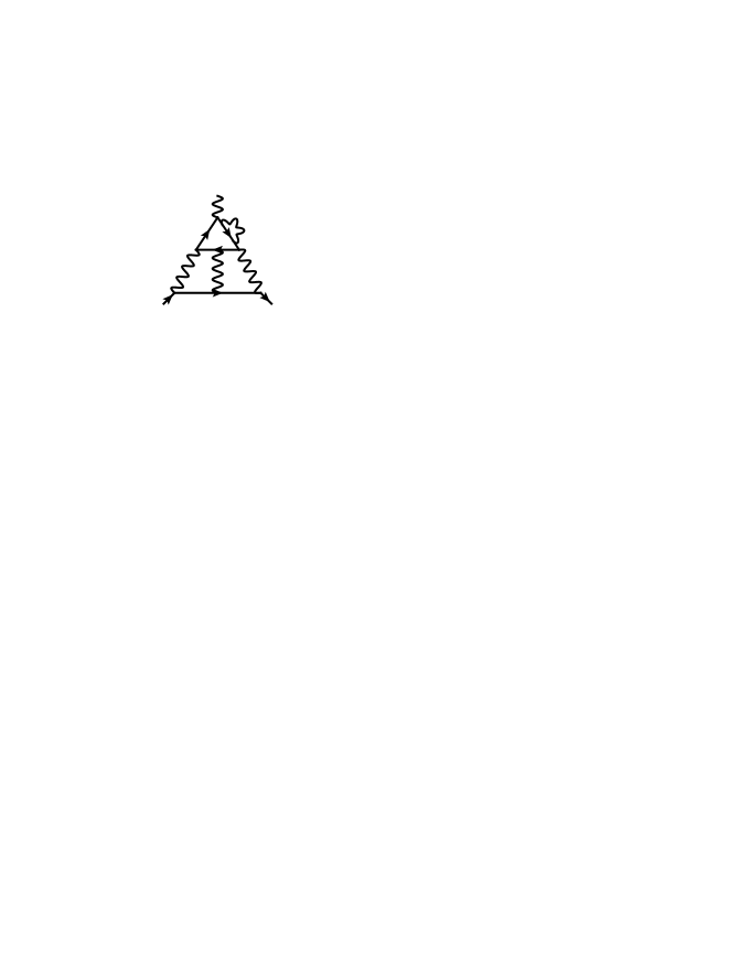
             3 loops IV(a) IV(b) IV(c)             

Figure 1: Sample light-by-light-type Feynman diagrams contributing to $a_{\mu}$. The external solid line represents the muon and at least one of the internal solid loops denotes electrons. In the case of IV(a) the second fermion loop can either be an electron or muon loop. Wavy lines represent photons.

It is convenient to decompose the four-loop term $a_{\mu}^{(8)}$ into a purely photonic piece and contributions involving electron and/or $\tau$ loops. Following Ref. [11] we write

$$a_{\mu}^{(8)} = A_{1}^{(8)}+A_{2}^{(8)}(m_{\mu}/m_{e})+A_{2}^{(8)}(m_{\mu}/m_{\tau})+A_{3}^{(8)}(m_{\mu}/m_{e},m_{\mu}/m_{\tau})\,.$$ (4)

$A_{2}^{(8)}(m_{\mu}/m_{\tau})$ has been computed in Ref. [41] using an asymptotic expansion for $m_{\mu}^{2}\ll m_{\tau}^{2}$. Analytic results have been obtained for several expansion terms which show a rapid convergence. $A_{2}^{(8)}(m_{\mu}/m_{\tau})$ and $A_{3}^{(8)}(m_{\mu}/m_{e},m_{\mu}/m_{\tau})$ are suppressed by $m_{\mu}^{2}/m_{\tau}^{2}$ and thus they are numerically small.

$A_{2}^{(8)}(m_{\mu}/m_{e})$ can be split into light-by-light-type contributions (cf. Fig. 1) and contributions where the external photon couples to the external muon line. The leading term of the latter can be obtained from calculations where in a first step the electron mass is set to zero and the fine structure constant is renormalized in the $\overline{\rm MS}$ scheme. Afterwards $\alpha$ is transformed to the on-shell scheme which introduces $\log(m_{e}/m_{\mu})$ terms in the final result. Using this approach, the non-light-by-light contributions with two closed electron loops have been computed analytically in Ref. [39].

In this paper we compute the four-loop light-by-light contributions to $A_{2}^{(8)}(m_{\mu}/m_{e})$ which are exemplified by three Feynman diagrams in Fig. 1. In case the external photon couples to a closed electron loop it is not possible to set $m_{e}=0$ since this generates infrared singularities. To circumvent this problem we perform an asymptotic expansion for $m_{e}\ll m_{\mu}$ which is described in some detail in Section 2. Results for contribution IV(a) with two closed electron loops have already been considered 40 years ago in Refs. [42, 43]. In Section 3 we will discuss in detail our results and compare to their findings and also to the ones in Ref. [11]. Section 4 contains our conclusions.

2 Technical details

The Feynman integrals which contribute to the light-by-light part of $A_{2}^{(8)}(m_{\mu}/m_{e})$ contain two widely separated scales, which provides a small expansion parameter

$$x = \frac{m_{e}}{m_{\mu}}\,\,\approx\,\,1/206.7682843\,.$$ (5)

Thus, it can be expected that already a few expansion terms provide a good approximation to the exact result. We compute four terms and show that the one of order $x^{3}$ leads to negligible contributions. The linear and quadratic term, however, can still lead to sizable contributions since the coefficients of $x^{n}$ contain $\log(x)\approx-5.3$ terms which at four-loop order are raised up to forth power.

We have implemented the asymptotic expansion using two different programs. In the first approach we use the Mathematica package asy [44, 45] which is based on expansion by regions [46, 47] formulated at the level of the alpha representation [48]. It provides the possibility to obtain the asymptotic behaviour of a Feynman diagram in a given limit. In fact, the output of asy are scaling rules for the alpha parameters. To exploit this information one has to find a distribution of the external momentum and the loop momenta obeying certain scaling rules which we obtain by trying out all possible combinations.

The second approach is based on an in-house program which generates all possible combinations of loop momenta and external momentum and assigns for each combination all possible scalings of the loop momenta (i.e. each loop momentum can either be soft or hard). In this way one obtains by construction all contributing regions. However, a double counting is introduced since the routing of the loop momenta is not unique. The double counting is eliminated with the help of the unique alpha representation which is generated for each momentum distribution.

We have applied both methods to each Feynman diagram and have obtained identical final results. Note, however, that asy requires significantly more CPU time than our in-house program which is tailored for the problem at hand.

The output of the asymptotic expansion is manipulated with FORM [49, 50] and TFORM [51] (see also Ref. [52]) which are used to perform traces and to deal with tensor structures. Afterwards only scalar integrals are left which are reduced to master integrals with the help of FIRE [53] and crusher [54]. For the classification of the master integrals we introduce the following set of propagators

$$P_{i}=\left\{\frac{1}{k^{2}},\frac{1}{k^{2}-M^{2}},\frac{1}{k^{2}-2k\cdot q},\frac{1}{2k\cdot q}\right\}\,,\qquad M\in\{m_{e},m_{\mu}\}\,,$$ (6)

where $k$ is a linear combination of loop momenta and $q$, the external momentum, with $q^{2}=m_{\mu}^{2}$. Using these propagators we can build the required three integral classes

Vacuum integrals

$$V(i_{1},...,i_{n})=\int\left(\prod_{j=1}^{L}d^{D}k_{j}\right)D_{1}^{i_{1}}\cdots D_{n}^{i_{n}},\,\qquad D_{i}\in\{P_{1},P_{2}\}\,,$$ (7)

On-shell integrals

$$O(i_{1},...,i_{n})=\int\left(\prod_{j=1}^{L}d^{D}k_{j}\right)D_{1}^{i_{1}}\cdots D_{n}^{i_{n}},\,\qquad D_{i}\in\{P_{1},P_{2},P_{3}\}\,,$$ (8)

Linear integrals

$$L(i_{1},...,i_{n})=\int\left(\prod_{j=1}^{L}d^{D}k_{j}\right)D_{1}^{i_{1}}\cdots D_{n}^{i_{n}},\,\qquad D_{i}\in\{P_{1},P_{2},P_{4}\}\,,$$ (9)

which are exemplified in Fig. 2.

Figure 2: Sample Feynman diagrams for the three appearing integral classes introduced in Eqs. (7) (left), (8) (middle) and (9) (right). Solid and dashed lines denote massive and massless propagators. Double lines stand for denominators of the form $1/(2k\cdot q)$.

To get an impression how the individual types of integrals arise after asymptotic expansion we discuss in some detail the three-loop case (cf. left diagram in Fig. 1). The valid regions are obtained by considering appropriate routings of the loop and external momenta, allowing each loop momentum to be either soft ($k\sim m_{e}$) or hard ($k\sim m_{\mu}$). In total we obtain eight possible regions. In case all loop momenta are hard the electron propagators are expanded in $m_{e}$ and one ends up with three-loop on-shell integrals. On the other hand, in case all loop momenta are soft the muon propagators are expanded for $k^{2}\ll 2k\cdot q$ and one has

$$\frac{1}{m_{\mu}^{2}-(k-q)^{2}} = \frac{1}{2k\cdot q-k^{2}}\,\,=\,\,\frac{1}{2k\cdot q}\left(1+\frac{k^{2}}{2k\cdot q}+\ldots\right)\,,$$ (10)

which leads to linear integrals where $m_{e}$ sets the mass scale. If two loop momenta are hard and one is soft one obtains two-loop on-shell (with mass scale $m_{\mu}$) and one-loop vacuum integrals (with mass scale $m_{e}$). The remaining three regions, i.e. two soft and one hard loop momentum, leads to one-loop on-shell integrals and either vacuum or linear integrals where the massive scale is given by the electron mass. It is interesting to note that on-shell and vacuum integrals only occur for the even powers of $x$ whereas linear integrals are present both for even and odd powers. Note, however, that the corresponding master integrals differ: the $x^{0}$ and $x^{2}$ terms involve master integrals with even number of linear propagators whereas for the $x^{1}$ and $x^{3}$ terms their number is odd.

The pattern observed at three loops repeats itself at four loops. For some diagrams one obtains more than 20 regions leading to single-scale integrals of the type

• four-loop on-shell,

• four-loop linear,

• products of three-loop on-shell and one-loop vacuum,

• products of two-loop on-shell and two-loop vacuum or linear,

• products of one-loop on-shell and three-loop vacuum or linear,

• and products two one-loop and one two-loop integrals involving vacuum, on-shell and/or linear integrals.

The mass scale of the on-shell integrals is given by $m_{\mu}$ and the one of the vacuum and linear integrals by $m_{e}$, with the following exception: one-loop vacuum integrals with mass scale $m_{\mu}$ occur in IV(a) in case a closed muon loop is present.

Massive vacuum integrals, which are only needed up to three loops, are well documented in the literature [55, 56]. All one-, two- and three-loop on-shell integrals entering our calculation are known analytically [57]. There are about 70 four-loop on-shell integral which are needed for IV(a), IV(b) and IV(c), about 40 are known analytically or to high numerical precision. All of them are taken from the calculation of the four-loop $\overline{\rm MS}$-on-shell quark mass relation performed in Ref. [58]. We furthermore require about 70 four-loop linear master integrals where about 20 have been computed analytically or to high numerical precision using Mellin-Barnes techniques [59]. The remaining ones have been computed using the package FIESTA [60]. We propagate the uncertainty from each $\epsilon$ coefficient of each master integral to the final result. To obtain the final error estimate we add the uncertainties in quadrature.

The renormalization of the light-by-light contribution only involves one-loop on-shell counterterms for the fine structure constant, the muon and electron masses and the wave function which are well established in the literature (see, e.g., the textbook [61]).

3 Discussion of results

We start with looking at the three-loop light-by-light contribution to $A_{2}^{(6)}(m_{\mu}/m_{e})$ which is known analytically [8]. Using the method described in the previous section we obtain in numerical form ($x=m_{e}/m_{\mu}$)

$$A_{2,\rm lbl}^{(6)}(m_{\mu}/m_{e}) = -14.5525-6.5797\ell_{x}$$ (11)

$$\mbox{}+x\left[18.0169-13.1595\ell_{x}\right]$$

$$\mbox{}+x^{2}\left[-12.4582+1.5944\ell_{x}-5.5700\ell_{x}^{2}+0.6667\ell_{x}^{3}\right]$$

$$\mbox{}+x^{3}\left[-12.0628-10.9662\ell_{x}\right]$$

$$\mbox{}+x^{4}\left[14.4529-19.0431\ell_{x}+2.2778\ell_{x}^{2}-0.7778\ell_{x}^{3}\right]$$

$$= -14.5525+35.0805$$

$$\mbox{}+\left[0.08714+0.3393\right]$$

$$\mbox{}+\left[-0.0002914-0.0001988-0.003703-0.002363\right]$$

$$\mbox{}+\left[-0.0000014+0.0000066\right]$$

$$\mbox{}+\left[0.0000000079+0.000000056+0.000000035+0.000000064\right]$$

$$= 20.5280+0.4265-0.006557+0.0000052+0.0000002$$

$$= 20.9479\,,$$

where terms of order $x^{5}$ are neglected and $\ell_{x}=\log(x)\approx-5.3$. For completeness we provide analytic results in the Appendix. One observes that odd powers in $x$ contain at most linear terms in $\ell_{x}$ whereas even powers contain terms up to $\ell_{x}^{3}$. After the second equality sign the numerical value for $x$ is inserted, however, the contribution from the various powers of $x$ and $\ell_{x}$ are kept separately. At order $x^{0}$ and $x^{1}$ the logarithmic contribution dominates over the constant. At order $x^{2}$ the constant and linear logarithmic term is of the same order of magnitude and about a factor ten smaller than the quadratic and cubic contribution. After the third equality sign all contributions to $x^{n}$ are added. One observes that the overall contribution of the $x^{2}$ term is already quite small and amounts to only 0.03% of the leading term. The linear term provides a 2% contribution and is still important. Let us mention that the cubic and quartic terms are below 0.00003% and are thus negligible. For completeness we present the final result for $A_{2,\rm lbl}^{(6)}(m_{\mu}/m_{e})$ after the last equality sign.

We now turn to the four-loop results. For convenience we split IV(a) into three contributions: IV(a0) contains two closed electron loops, in IV(a1) only the fermion loop with the coupling to the external photon contains electrons, and in IV(a2) electrons are running only in the two-point polarization function and muons in the other fermion loop. Let us mention that the coefficients of the logarithmic contributions in the case of IV(a0) are known analytically since the contributing four-loop on-shell integrals are available in the literature [39] and only the four-loop linear integrals have to be evaluated numerically. As a consequence, it is possible to reconstruct the pole terms of the IV(a0) contribution, which are in one-to-one correspondence to the coefficients of the logarithms, analytically. Similar arguments can be used to obtain the logarithmic contributions of IV(a1) and IV(a2), for the $x^{1}$ and $x^{3}$ terms of IV(b) and for the $x^{0}$, $x^{1}$ and $x^{3}$ terms of IV(c). They are given in the Appendix. In the main part of the paper we restrict ourselves to numerical results.

Using the same scheme for presenting the results as in Eq. (11) we obtain for the five four-loop light-by-light-type contributions

$$A_{2}^{(8),\rm IV(a0)} = 7.5018\pm 0.0026+14.8808\ell_{x}+6.5797\ell_{x}^{2}$$ (12)

$$\mbox{}+x\left[6.29\pm 0.46-14.6216\ell_{x}+8.7729\ell_{x}^{2}\right]$$

$$\mbox{}+x^{2}\left[-16.81\pm 0.43+30.0172\ell_{x}-6.5069\ell_{x}^{2}+7.6489\ell_{x}^{3}-0.8889\ell_{x}^{4}\right]$$

$$\mbox{}+x^{3}\left[-48.31\pm 0.24-4.8739\ell_{x}+13.1595\ell_{x}^{2}\right]$$

$$= 7.5018\pm 0.0026-79.3384+187.0352$$

$$\mbox{}+\left[0.0304\pm 0.0022+0.3770+1.2061\right]$$

$$\mbox{}+\left[-0.000393\pm 0.000010-0.003743-0.004326-0.02711-0.01680\right]$$

$$\mbox{}+\left[-0.0000055+0.0000029+0.0000423\right]$$

$$= \left[115.1986\pm 0.0026\right]+\left[1.6135\pm 0.0022\right]+\left[-0.052378\pm 0.000010\right]$$

$$\mbox{}\qquad\qquad+\left[0.000040\right]$$

$$= 116.7598\pm 0.0034\,,$$

$$A_{2}^{(8),\rm IV(a1)} = 2.734\pm 0.028$$ (13)

$$\mbox{}+x\left[-9.5571\right]$$

$$\mbox{}+x^{2}\left[-7.494\pm 0.033-14.2010\ell_{x}+0.3559\ell_{x}^{2}\right]$$

$$\mbox{}+x^{3}\left[6.1668-9.0654\ell_{x}\right]$$

$$= 2.734\pm 0.028$$

$$\mbox{}+\left[-0.04622\right]$$

$$\mbox{}+\left[-0.000175\pm 0.000001+0.001771+0.0002366\right]$$

$$\mbox{}+\left[0.000001+0.000005\right]$$

$$= \left[2.734\pm 0.028\right]+\left[-0.04622\right]+\left[0.001832\pm 0.000001\right]+\left[0.000006\right]$$

$$= 2.690\pm 0.028\,,$$

$$A_{2}^{(8),\rm IV(a2)} = 0.370\pm 0.033-0.7420\ell_{x}$$ (14)

$$\mbox{}+x\left[0\right]$$

$$\mbox{}+x^{2}\left[0.8628\pm 0.002618\right]$$

$$\mbox{}+x^{3}\left[-2.6844\right]$$

$$= +\left[0.370\pm 0.033+3.9561\right]$$

$$\mbox{}+\left[0\right]$$

$$\mbox{}+\left[0.00002018\pm 0.00000006\right]$$

$$\mbox{}+\left[-0.0000003\right]$$

$$= +\left[4.326\pm 0.03288\right]+\left[0\right]+\left[0.00002018\pm 0.00000006\right]+\left[-0.0000003\right]$$

$$= 4.326\pm 0.033\,,$$

$$A_{2}^{(8),\rm IV(b)} = 27.395\pm 0.014+(4.93482\pm 0.00003)\ell_{x}$$ (15)

$$\mbox{}+x\left[-0.81\pm 1.22+59.0235\ell_{x}\right]$$

$$\mbox{}+x^{2}\left[142.5\pm 7.6+40.6546\ell_{x}+20.5582\ell_{x}^{2}-9.6167\ell_{x}^{3}+0.8333\ell_{x}^{4}\right]$$

$$\mbox{}+x^{3}\left[62.11\pm 2.89+132.7421\ell_{x}-40.9406\ell_{x}^{2}\right]$$

$$= 27.395\pm 0.014+(-26.3105\pm 0.0002)$$

$$\mbox{}+\left[-0.0039\pm 0.0059-1.5219\right]$$

$$\mbox{}+\left[0.003334\pm 0.0001769-0.005070+0.01367+0.03409+0.01575\right]$$

$$\mbox{}+\left[0.000007\pm 0.-0.000080-0.000132\right]$$

$$= \left[1.084\pm 0.014\right]+\left[-1.5259\pm 0.0059\right]+\left[0.06177\pm 0.00018\right]+\left[-0.0002047\right]$$

$$= -0.380\pm 0.016\,,$$

$$A_{2}^{(8),\rm IV(c)} = -14.900\pm 0.059-3.2899\ell_{x}$$ (16)

$$\mbox{}+x\left[65.4209\right]$$

$$\mbox{}+x^{2}\left[33.61\pm 9.96+(56.76\pm 0.78)\ell_{x}+(-24.66\pm 0.27)\ell_{x}^{2}\right.$$

$$\left.\qquad\qquad+(-1.935\pm 0.091)\ell_{x}^{3}\right]$$

$$\mbox{}+x^{3}\left[25.11\pm 0.60+107.4325\ell_{x}-19.8610\ell_{x}^{2}\right]$$

$$= -14.9\pm 0.05945+17.54$$

$$\mbox{}+\left[0.3164\right]$$

$$\mbox{}+\left[0.00079\pm 0.00023+(-0.007078\pm 0.000097)\right.$$

$$\left.\qquad\qquad+(-0.01640\pm 0.00018)+(0.00686\pm 0.00032)\right]$$

$$\mbox{}+\left[0.00000284\pm 0.00000007-0.00006479-0.00006387\right]$$

$$= \left[2.641\pm 0.059\right]+\left[0.3164\right]+\left[-0.01583\pm 0.00045\right]$$

$$\qquad\qquad+\left[-0.00012582\pm 0.00000007\right]$$

$$= 2.941\pm 0.059\,,$$

where the uncertainties origin from the numerical integration using FIESTA. It is common to all five cases that the $x^{3}$ term only provides a negligible contribution of at most 0.05% [in the case of IV(b)] which is much smaller than the uncertainty estimate of the leading $x^{0}$ term. In most cases the $x^{2}$ terms lead to contributions comparable to the numerical uncertainty of the leading term. Together with the $x^{3}$ terms they confirm the good convergence property of the asymptotic expansion. It is nevertheless interesting to note that in general the cubic and quartic logarithms of the $x^{2}$ term lead to the largest numerical contributions, however, also the quadratic $\log(x)$ terms are not negligible.

In the linear mass correction terms we observe logarithmic contributions up to second order. They lead to significantly larger numerical contributions than the linear logarithms which are in turn much larger than the constant.

In the leading term only IV(a0) has a quadratic logarithm, one from each electron loop. The $\log^{2}(x)$ term provides the numerical dominant contribution, however, more than 40% are canceled by the linear logarithm; the constant term is an order of magnitude smaller. Linear logarithmic terms are also present for IV(a2), IV(b) and IV(c). In the latter two cases strong cancellations between the $\log(x)$ and the constant are observed, which leads to an interesting effect for IV(b): the leading term is smaller than the $m_{e}/m_{\mu}$-suppressed term. As a consequence the final numerical result for IV(b) is quite small and has a big relative uncertainty.

$A_{2}^{(8)}(m_{\mu}/m_{e})$	this work	[35, 11]	[42]	[43]
IV(a0)	$116.76\pm 0.02$	$116.759183\pm 0.000292$	$111.1\pm 8.1$	$117.4\pm 0.5$
IV(a1)	$2.69\pm 0.14$	$2.697443\pm 0.000142$
IV(a2)	$4.33\pm 0.17$	$4.328885\pm 0.000293$
IV(a)	$123.78\pm 0.22$	$123.78551\hphantom{2}\pm 0.00044\hphantom{2}$
IV(b)	$-0.38\pm 0.08$	$-0.4170\hphantom{22}\pm 0.0037\hphantom{22}$
IV(c)	$2.94\pm 0.30$	$2.9072\hphantom{22}\pm 0.0044\hphantom{22}$

Table 1: Summary of the final results for the individual four-loop light-by-light-type contributions and their comparison with results from the literature. Note that the uncertainties given in the second column are obtained from Eqs. (12) to (16) after multiplication by five.

In Table 1 we summarize our findings for IV(a0), IV(a1), IV(a2), IV(b) and IV(c) and compare with the literature. To be on the conservative side we multiply the Monte-Carlo uncertainty from Eqs. (12) to (16) by a factor of five. For all classes under consideration we find good agreement with previous results. For the dominant contribution IV(a) we find excellent agreement.

Although our numerical precision can not compete with the one of Ref. [11], let us note that our computation procedure is completely different from the numerical method used in [11]. As our calculation is a second evaluation of the complete light-by-light contribution to $A_{2}^{(8)}(m_{\mu}/m_{e})$, our result is an important check of the existing value. Furthermore, since the asymptotic expansion and the reduction to master integrals were done analytically, it is possible to systematically improve the precision by evaluating more and more master integrals analytically.

4 Conclusions

We have computed the four-loop QED corrections to the muon magnetic moment induced by the light-by-light-type Feynman diagrams involving a closed electron loop. This is a finite and gauge invariant subset, which provides about 95% of the total four-loop contribution. Our results for the individual sub-classes IV(a), IV(b) and IV(c) agree with the literature [11].

We want to stress that our approach is completely different from the one of Ref. [11] and thus should be considered as an independent cross check. We perform an analytic reduction of all occurring integrals to a small set of master integrals which are then computed using analytical or numerical methods. In particular all counterterm contributions are available analytically. On the other hand, in Ref. [11] infrared and ultraviolet finite multi-dimensional integrands for the individual sub-classes of $a_{\mu}^{(8)}$ are constructed which are then integrated numerically.

Our final results can be found in Table 1. Although our numerical uncertainty, which amounts to approximately $0.4\times(\alpha/\pi)^{4}\approx 1.2\times 10^{-11}$, is larger than the one of Ref. [11], it is still much smaller than the difference between the theory prediction and experimental result of $a_{\mu}$ [cf. Eq. (3)]. We also want to note that our result can be systematically improved by evaluating more and more master integrals analytically.

Appendix: Selected analytic three- and four-loop results for $a_{\mu}$

In this appendix we provide analytic results for the three-loop light-by-light contribution $A_{2,\rm lbl}^{(6)}(m_{\mu}/m_{e})$ and for some of the four-loop contributions.

The analytic version of Eq. (11) reads

$$A_{2,\rm lbl}^{(6)}(m_{\mu}/m_{e})=\ x^{0}\ \left(\frac{2}{3}-\frac{10\pi^{2}}{3}+\frac{59\pi^{4}}{270}-3\zeta_{3}-\frac{2\pi^{2}}{3}\ \ell_{x}\right)$$

$$+x\left(\frac{424\pi^{2}}{9}-\frac{196\ln(2)\pi^{2}}{3}-\frac{4\pi^{2}}{3}\ \ell_{x}\right)$$

$$+x^{2}\ \Bigg{[}-\frac{283}{12}+\frac{25\pi^{2}}{18}-\frac{61\pi^{4}}{270}+3\zeta_{3}+\frac{4\pi^{2}\zeta_{3}}{3}$$

$$+\left(\frac{61}{3}-\frac{32\pi^{2}}{9}+\frac{16\pi^{4}}{135}+4\zeta_{3}\right)\ \ell_{x}+\left(\frac{\pi^{2}}{9}-\frac{20}{3}\right)\ \ell_{x}^{2}+\frac{2}{3}\ \ell_{x}^{3}\Bigg{]}$$

$$+x^{3}\ \left(-\frac{11\pi^{2}}{9}-\frac{10\pi^{2}}{9}\ \ell_{x}\right)$$

$$+x^{4}\ \left[\frac{13283}{2592}+\frac{191\pi^{2}}{216}+\frac{\zeta_{3}}{2}+\left(-\frac{517}{108}-\frac{13\pi^{2}}{9}\right)\ \ell_{x}+\frac{41}{18}\ \ell_{x}^{2}-\frac{7}{9}\ \ell_{x}^{3}\right]\,.$$ (17)

where $\zeta_{n}$ is Riemann’s zeta function evaluated at $n$.

At four-loop order one can obtain analytic results for the coefficients of $\ell_{x}^{n}$ ($n\geq 1$) for IV(a0), IV(a1) and IV(a2), for the $x^{1}$ and $x^{3}$ terms of IV(b) and for the $x^{0}$, $x^{1}$ and $x^{3}$ terms of IV(c). These contributions are given by

$$A_{2}^{\text{(8),IV(a0)}}|_{\ell_{x}}=\ \left(-\frac{4}{3}+\frac{8\pi^{2}}{3}-\frac{8\pi^{4}}{45}+6\zeta_{3}\right)\ \ell_{x}+\frac{2\pi^{2}}{3}\ \ell_{x}^{2}$$

$$+x\left(\frac{-40\pi^{2}}{27}\ \ell_{x}+\frac{8\pi^{2}}{9}\ \ell_{x}^{2}\right)$$

$$+x^{2}\ \Bigg{[}\left(\frac{47}{3}+6\pi^{2}-\frac{98\pi^{4}}{405}-10\zeta_{3}-\frac{8\pi^{2}\zeta_{3}}{27}-\frac{50\zeta_{5}}{9}\right)\ \ell_{x}$$

$$+\left(-\frac{220}{9}+\frac{32\pi^{2}}{9}-\frac{16\pi^{4}}{135}-\frac{14\zeta_{3}}{3}\right)\ \ell_{x}^{2}+\left(\frac{82}{9}-\frac{4\pi^{2}}{27}\right)\ \ell_{x}^{3}-\frac{8}{9}\ \ell_{x}^{4}\Bigg{]}$$

$$+x^{3}\ \left(\frac{-40\pi^{2}}{81}\ \ell_{x}+\frac{4\pi^{2}}{3}\ \ell_{x}^{2}\right)\,,$$ (18)

$$A_{2}^{\text{(8),IV(a1)}}|_{\ell_{x}}=\ x^{2}\ \left(\frac{137}{27}-\frac{12629\pi^{2}}{9720}-\frac{2\ln(2)\pi^{2}}{3}-\frac{31\pi^{4}}{405}+\frac{125\zeta_{3}}{27}\right)\ \ell_{x}$$

$$+x^{2}\ \left(\frac{\pi^{2}}{9}-\frac{20}{27}\right)\ \ell_{x}^{2}-x^{3}\ \frac{124\pi^{2}}{135}\ \ell_{x}\,,$$ (19)

$$A_{2}^{\text{(8),IV(a2)}}|_{\ell_{x}}=\ \bigg{(}-\frac{10}{9}-32a_{4}-\frac{4\ln^{4}(2)}{3}-\frac{931\pi^{2}}{27}+48\ln(2)\pi^{2}$$

$$+\frac{4\ln^{2}(2)\pi^{2}}{3}+\frac{41\pi^{4}}{270}+\frac{8\zeta_{3}}{3}+\frac{5\pi^{2}\zeta_{3}}{9}-\frac{5\zeta_{5}}{3}\bigg{)}\ \ell_{x}\,,$$ (20)

$$A_{2}^{\text{(8),IV(b)}}|_{x^{1},\ell_{x}}=\ x\left(3\pi^{3}-\frac{31\pi^{2}}{9}\right)\ \ell_{x}\,,$$ (21)

$$A_{2}^{\text{(8),IV(b)}}|_{x^{3},\ell_{x}}=\ x^{3}\left[\left(\frac{137\pi^{2}}{4050}+\frac{1153\pi^{3}}{270}\right)\ \ell_{x}-\frac{112\pi^{2}}{27}\ \ell_{x}^{2}\right]\,,$$ (22)

$$A_{2}^{\text{(8),IV(c)}}|_{x^{0},\ell_{x}}=\ -\frac{\pi^{2}}{3}\ \ell_{x}\,,$$ (23)

$$A_{2}^{\text{(8),IV(c)}}|_{x^{1},\ell_{x}}=\ 0\,,$$ (24)

$$A_{2}^{\text{(8),IV(c)}}|_{x^{3},\ell_{x}}=\ x^{3}\left[\frac{2939\pi^{2}}{270}\ \ell_{x}-\frac{163\pi^{2}}{81}\ \ell_{x}^{2}\right]\,,$$ (25)

with $a_{4}=\mbox{Li}_{4}(1/2)$.

References

- [1] G. W. Bennett et al. [Muon G-2 Collaboration], Phys. Rev. D 73 (2006) 072003 [hep-ex/0602035].
- [2] B. L. Roberts, Chin. Phys. C 34 (2010) 741 [arXiv:1001.2898 [hep-ex]].
- [3] R. M. Carey, K. R. Lynch, J. P. Miller, B. L. Roberts, W. M. Morse, Y. K. Semertzides, V. P. Druzhinin and B. I. Khazin et al., FERMILAB-PROPOSAL-0989.
- [4] T. Mibe [J-PARC g-2 Collaboration], Chin. Phys. C 34 (2010) 745.
- [5] K. Melnikov and A. Vainshtein, Springer Tracts Mod. Phys. 216 (2006) 1.
- [6] F. Jegerlehner and A. Nyffeler, Phys. Rept. 477 (2009) 1 [arXiv:0902.3360 [hep-ph]].
- [7] J. P. Miller, E. d. Rafael, B. L. Roberts and D. Stöckinger, Ann. Rev. Nucl. Part. Sci. 62 (2012) 237.
- [8] S. Laporta and E. Remiddi, Phys. Lett. B 301 (1993) 440.
- [9] S. Laporta, Nuovo Cim. A 106 (1993) 675.
- [10] S. Laporta and E. Remiddi, Phys. Lett. B 379 (1996) 283 [hep-ph/9602417].
- [11] T. Aoyama, M. Hayakawa, T. Kinoshita and M. Nio, Phys. Rev. Lett. 109 (2012) 111808 [arXiv:1205.5370 [hep-ph]].
- [12] A. Czarnecki, B. Krause and W. J. Marciano, Phys. Rev. Lett. 76 (1996) 3267 [hep-ph/9512369].
- [13] M. Knecht, S. Peris, M. Perrottet and E. De Rafael, JHEP 0211 (2002) 003 [hep-ph/0205102].
- [14] A. Czarnecki, W. J. Marciano and A. Vainshtein, Phys. Rev. D 67 (2003) 073006 [Phys. Rev. D 73 (2006) 119901] [hep-ph/0212229].
- [15] C. Gnendiger, D. Stöckinger and H. Stöckinger-Kim, Phys. Rev. D 88 (2013) 053005 [arXiv:1306.5546 [hep-ph]].
- [16] M. Davier, A. Hoecker, B. Malaescu and Z. Zhang, Eur. Phys. J. C 71 (2011) 1515 [Erratum-ibid. C 72 (2012) 1874] [arXiv:1010.4180 [hep-ph]].
- [17] K. Hagiwara, R. Liao, A. D. Martin, D. Nomura and T. Teubner, J. Phys. G 38 (2011) 085003 [arXiv:1105.3149 [hep-ph]].
- [18] F. Jegerlehner and R. Szafron, Eur. Phys. J. C 71 (2011) 1632 [arXiv:1101.2872 [hep-ph]].
- [19] M. Benayoun, P. David, L. DelBuono and F. Jegerlehner, Eur. Phys. J. C 73 (2013) 2453 [arXiv:1210.7184 [hep-ph]].
- [20] B. Krause, Phys. Lett. B 390 (1997) 392 [hep-ph/9607259].
- [21] D. Greynat and E. de Rafael, JHEP 1207 (2012) 020 [arXiv:1204.3029 [hep-ph]].
- [22] K. Hagiwara, A. D. Martin, D. Nomura and T. Teubner, Phys. Rev. D 69 (2004) 093003 [hep-ph/0312250].
- [23] A. Kurz, T. Liu, P. Marquard and M. Steinhauser, Phys. Lett. B 734 (2014) 144 [arXiv:1403.6400 [hep-ph]].
- [24] A. Nyffeler, Phys. Rev. D 79 (2009) 073012 [arXiv:0901.1172 [hep-ph]].
- [25] K. Melnikov and A. Vainshtein, Phys. Rev. D 70 (2004) 113006 [hep-ph/0312226].
- [26] J. Bijnens and J. Prades, Mod. Phys. Lett. A 22 (2007) 767 [hep-ph/0702170 [HEP-PH]].
- [27] G. Colangelo, M. Hoferichter, A. Nyffeler, M. Passera and P. Stoffer, Phys. Lett. B 735 (2014) 90 [arXiv:1403.7512 [hep-ph]].
- [28] J. S. Schwinger, Phys. Rev. 73 (1948) 416.
- [29] A. Petermann, Helv. Phys. Acta 30 (1957) 407.
- [30] C. M. Sommerfield, Phys. Rev. 107 (1957) 328.
- [31] H.H. Elend, Phys. Lett. 20 (1966) 682; 21 (1966) 720(E).
- [32] M. A. Samuel and G. -w. Li, Phys. Rev. D 44 (1991) 3935 [Erratum-ibid. D 48 (1993) 1879].
- [33] A. Czarnecki and M. Skrzypek, Phys. Lett. B 449 (1999) 354 [hep-ph/9812394].
- [34] M. Passera, Phys. Rev. D 75 (2007) 013002 [hep-ph/0606174].
- [35] T. Kinoshita and M. Nio, Phys. Rev. D 70 (2004) 113001 [hep-ph/0402206].
- [36] T. Aoyama, M. Hayakawa, T. Kinoshita and M. Nio, Phys. Rev. D 77 (2008) 053012 [arXiv:0712.2607 [hep-ph]].
- [37] S. Laporta, Phys. Lett. B 312 (1993) 495 [hep-ph/9306324].
- [38] J. -P. Aguilar, D. Greynat and E. De Rafael, Phys. Rev. D 77 (2008) 093010 [arXiv:0802.2618 [hep-ph]].
- [39] R. Lee, P. Marquard, A. V. Smirnov, V. A. Smirnov and M. Steinhauser, JHEP 1303 (2013) 162 [arXiv:1301.6481 [hep-ph]].
- [40] P. A. Baikov, K. G. Chetyrkin, J. H. Kuhn, C. Sturm, Nucl. Phys. B 867 (2013) 182 [arXiv:1207.2199 [hep-ph]].
- [41] A. Kurz, T. Liu, P. Marquard and M. Steinhauser, Nucl. Phys. B 879 (2014) 1 [arXiv:1311.2471 [hep-ph]].
- [42] J. Calmet and A. Peterman, Phys. Lett. B 56 (1975) 383.
- [43] C. Chlouber and M. A. Samuel, Phys. Rev. D 16 (1977) 3596.
- [44] A. Pak and A. Smirnov, Eur. Phys. J. C 71 (2011) 1626 [arXiv:1011.4863 [hep-ph]].
- [45] B. Jantzen, A. V. Smirnov and V. A. Smirnov, Eur. Phys. J. C 72 (2012) 2139 [arXiv:1206.0546 [hep-ph]].
- [46] M. Beneke and V. A. Smirnov, Nucl. Phys. B 522 (1998) 321 [hep-ph/9711391].
- [47] V. A. Smirnov, Springer Tracts Mod. Phys. 177 (2002) 1.
- [48] V. A. Smirnov, Phys. Lett. B 465 (1999) 226 [hep-ph/9907471].
- [49] J. A. M. Vermaseren, arXiv:math-ph/0010025.
- [50] J. Kuipers, T. Ueda, J. A. M. Vermaseren and J. Vollinga, Comput. Phys. Commun. 184 (2013) 1453 [arXiv:1203.6543 [cs.SC]].
- [51] M. Tentyukov and J. A. M. Vermaseren, Comput. Phys. Commun. 181 (2010) 1419 [hep-ph/0702279].
- [52] M. Steinhauser, T. Ueda and J. A. M. Vermaseren, Nucl. Part. Phys. Proc. 261-262 45 [arXiv:1501.07119 [hep-ph]].
- [53] A. V. Smirnov, Comput. Phys. Commun. 189 (2014) 182 [arXiv:1408.2372 [hep-ph]].
- [54] P. Marquard, D. Seidel, unpublished.
- [55] L. V. Avdeev, Comput. Phys. Commun. 98 (1996) 15 [hep-ph/9512442].
- [56] M. Steinhauser, Comput. Phys. Commun. 134 (2001) 335 [hep-ph/0009029].
- [57] R. N. Lee and V. A. Smirnov, JHEP 1102 (2011) 102 [arXiv:1010.1334 [hep-ph]].
- [58] P. Marquard, A. V. Smirnov, V. A. Smirnov and M. Steinhauser, Phys. Rev. Lett. 114 (2015) 14, 142002 [arXiv:1502.01030 [hep-ph]].
- [59] M. Czakon, Comput. Phys. Commun. 175 (2006) 559 [hep-ph/0511200].
- [60] A. V. Smirnov, Comput. Phys. Commun. 185 (2014) 2090 [arXiv:1312.3186 [hep-ph]].
- [61] L. H. Ryder, Cambridge, Uk: Univ. Pr. ( 1985) 443p
- [62] V. Sadovnichy, A. Tikhonravov, V. Voevodin, and V. Opanasenko, “‘Lomonosov’: Supercomputing at Moscow State University.” In Contemporary High Performance Computing: From Petascale toward Exascale (Chapman & Hall/CRC Computational Science), pp.283-307, Boca Raton, USA, CRC Press, 2013.