Synchronization of qubit ensemble under optimized $\pi$-pulse driving

Abstract

We propose technique of simultaneous excitation of disordered qubits providing an effective suppression of inhomogeneous broadening in their spectral density. The technique is based on applying of optimally chosen $\pi$-pulse with non-rectangular smooth shape. We study excitation dynamics of an off-resonant qubit subjected to strong classical electromagnetic driving field with the fast reference frequency and slow envelope. Within this solution we optimize the envelope to achieve a preassigned accuracy in qubit synchronization.

I Introduction

The investigation of qubit ensembles reveals analogies with quantum optics effects Blais ; YouNori ; Astafiev and possibilities for construction of quantum computers and simulators DiCarlo ; MSS ; Nation ; Clarke . Solid state realizations of qubit ensembles are superconducting Josephson circuits MSS ; Orlando ; mooij , nitrogen-vacancy (NV) centers in diamond samples nv-centers-0 ; nv-centers ; nv-centers-1 , or nuclear and electron spins realized as ³¹P donors in ²⁸Si crystals Morton and Cr³⁺ spins in Al₂O₃ Schuster . The coupling of qubit ensembles with a superconducting microwave resonators results in the formation of sub-wavelength quantum metamaterials Macha ; Rakhmanov ; Fistul ; ZKF ; SMRU . The long-range interaction through a photon mode results in the formation of collective qubit states in such metamaterials Brandes ; Zou , as Dicke model describes. One of crucial distinctions of artificial qubits from natural atoms is that their excitation energies are in many cases tunable in situ by external magnetic fields. Beside of the tunability, another property is a disorder in excitation frequencies and, as a consequence, inhomogeneous broadening of the density of states in qubit ensembles. This is related to fundamental mechanisms such as exponential dependence of excitation energy on Josephson and charging energies in superconducting qubits or spatial fluctuations of background magnetic moments Stanwix in systems with NV-centers.

Disordered spectrum of collective modes offers multimode quantum memory, where information about photon state is encoded as a tunable collective qubit mode Wesenberg0 ; Wesenberg . The storage and retrieval protocols were proposed in Refs. Moelmer ; Grezes ; Wu and based on spin-refocusing techniques spinref-1 ; spinref-2 or successive magnetic field gradients. In the context of quantum memory the unavoidable spectral broadening in qubit excitation frequencies provides multimode performance from one side, but from the other side this is one of limiting factors affecting coherence times. Therefore, the development of techniques of effective suppression of the disorder in qubit frequencies and synchronization of their dynamics is an important problem. For instance, one of the options is atomic frequency comb (AFC) technique which could be applied to rare-earth-metal-ion qubit ensembles ASRG . This method is based on frequency-selective optical pumping and subsequent transitions to metastable auxiliary hyperfine states. Another way of solution of this problem was demonstrated in Ref. nv-centers as ’cavity protection’ effect in NV-centers. The effect is related to a decreasing of a relaxation rate of collective qubit modes which is proportional to the spectral broadening.

Our research is inspired by one of the key ideas of Ref. nv-centers : the succession of microwave rectangular pulses can serve as efficient method for excitation of disordered NV-centers from the ground to the excited state. In our paper we study the possibility of simultaneous qubit excitation by a single non-rectangular $\pi$-pulse, rather than the sequence mentioned above. We observe that the optimized non-rectangular shape of $\pi$-pulse provides an efficient tool for suppression of the disorder effects as well. It allows to excite qubits within a wide detuning range with almost 100% probability. In contrast to AFC methods, this technique does not require using of auxiliary levels transitions.

We assume that the $\pi$-pulse is realized as electromagnetic signal $f(t)e^{-i\omega t}$ of a carrying frequency $\omega$ being almost in resonance with the qubit excitation frequency. In our solution we perform the optimization of the envelope shape $f(t)$ in an experimentally relevant class of smooth functions, which guarantees that higher energy levels of a qubit are not affected. We expect that this technique can be applied to disordered systems with strong qubit-cavity couplings like NV-centers or superconducting metamaterials, as well as to the atomic clock devices Hodges as a tool for the preparation of a particular atomic state.

II Definitions

We address to the possibility of simultaneous excitation of disordered qubit ensemble coupled to photon transmission line being the source of the driving. Qubits are assumed to be non-interacting with each other and long lived in comparison to $\pi$-pulse duration time $\tau\ll\tau_{\varphi}$. The absence of qubit-qubit interactions means that we can study dynamics of a single off-resonant driven qubit. We fix carrying frequency $\omega$ and assume that the qubit energy $\epsilon$ can be varied reflecting the spectral broadening. Neglecting the qubit decoherence we solve the Schrödinger equation only $i\partial_{t}|\psi\rangle=(H_{q}+H_{ext})|\psi\rangle$, where unperturbed qubit Hamiltonian is $H_{q}=\epsilon(\sigma_{0}+\sigma_{z})/2$ and the external driving is $H_{ext}=(f(t)e^{-i\omega t}\sigma_{+}+f^{*}(t)e^{i\omega t}\sigma_{-})/2$. We define wave function of the qubit state in $\omega$-rotating frame as

$$|\psi(t)\rangle=\begin{pmatrix}\alpha(t)e^{-i(\omega+\delta/2)t}\\[5.0pt] \beta(t)e^{-i\delta t/2}\end{pmatrix},$$

where the detuning frequency is $\delta=\epsilon-\omega$. The Hamiltonian $H$ of the driven qubit in this rotating frame reads

$$H=\frac{1}{2}\begin{pmatrix}\delta&&f(t)\\[5.0pt] f^{*}(t)&&-\delta\end{pmatrix}$$ (1)

We assume that the qubit is close to cavity resonance $\epsilon\approx\omega$ and consider the evolution of the qubit wave function within the time interval $0<t<\tau$ starting from the ground state $|\psi(0)\rangle=|g\rangle$ at the initial moment of time $t=0$. The $\pi$-pulse time $\tau$ is considered as a fixed value. At this point we define frequency

$$\Omega=\frac{\pi}{\tau},$$

which is the main scale in our consideration along with the detuning $\delta$. The frequency $\Omega$ has the transparent physical meaning: this is frequency of Rabi oscillations of the resonant qubit with $\delta=0$ under the constant driving amplitude given by $F_{0}(t)=\Omega e^{-i\omega t}$. Hence, time $\tau$ is the half of the Rabi period associated with rectangular $\pi$-pulse $F_{0}(0<t<\tau)$ exciting the system from $|g\rangle$ to $|e\rangle$. Non-zero detuning, related to inhomogeneous broadening or spread in qubit frequencies, does not allow to achieve full qubit excitation if envelope shape $f(t)$ is constant. In the following consideration we modify $f(t)$ at the time interval $0<t<\tau$ to more complicated non-rectangular shape $f(t)\neq\rm const$ to achieve higher efficiency in near-to-resonance qubit excitation.

Schrödinger equation with the Hamiltonian (1) allows analytical solutions only in several particular cases. The basic one is the constant driving amplitude $f(t)=f=\rm const$ and arbitrary detuning $\delta$ which corresponds to damped Rabi oscillations of the frequency $\Omega_{R}=\sqrt{f^{2}+\delta^{2}}$. In this case the evolution of the wave function being in the ground state at $t=0$ reads

$$|\psi(t)\rangle=\begin{pmatrix}-\frac{if}{\Omega_{R}}\sin\Omega_{R}t/2\\ \\ \cos\Omega_{R}t/2+\frac{i\delta}{\Omega_{R}}\sin\Omega_{R}t/2\end{pmatrix}.$$ (2)

One can see that detuning reduces the maximum of excitation probability. This effect results in impossibility of synchronization of qubit ensemble by the rectangular shape of the driving envelope.

Our further consideration is based on another exact solution, which holds for on-resonance driving regime $\delta=0$ and arbitrary real valued $f(t)$. The time evolution of the ground state within this solution reads

$$|\psi(t)\rangle=\begin{pmatrix}\displaystyle-i\sin\frac{\varphi(t)}{2}\\[10.00002pt] \displaystyle\cos\frac{\varphi(t)}{2}\end{pmatrix},$$ (3)

where the phase $\varphi(t)$ is given by the time integral

$$\varphi(t)=\int\limits_{0}^{t}f(t_{1})dt_{1}.$$

The $\pi$-pulse condition, which is the inversion of a qubit occupation number, for this resonant case holds for

$$\varphi(\tau)=\pi.$$ (4)

The last constraint (4) provides the class of real valued functions $f(t)$ we are addressed to in the optimization procedures below.

III Perturbative solution

As it was mentioned above, the exact solution is not known for arbitrary $f(t)$ and non-zero detuning $\delta\neq 0$. Hence, we develop a perturbation theory based on treating the $\delta\sigma_{z}/2$-terms in the Hamiltonian (1) as small perturbation and considering the exact solution (3) at $\delta=0$ as the zero order approximation. We end up with the following recursive equations forming the perturbation theory by $\delta$

$$i\dot{\alpha}^{(n)}(t)- \,\frac{f(t)}{2}\beta^{(n)}(t)=\frac{\delta}{2}\alpha^{(n-1)}(t)$$ (5)

$$i\dot{\beta}^{(n)}(t)- \,\frac{f(t)}{2}\alpha^{(n)}(t)=-\frac{\delta}{2}\beta^{(n-1)}(t).$$ (6)

The full solution reads

$$\begin{pmatrix}\alpha(t)\\[10.00002pt] \beta(t)\end{pmatrix}=\begin{pmatrix}\displaystyle x(t)\cos\frac{\varphi(t)}{2}-iy(t)\sin\frac{\varphi(t)}{2}\\[10.00002pt] \displaystyle y(t)\cos\frac{\varphi(t)}{2}-ix(t)\sin\frac{\varphi(t)}{2}\end{pmatrix}.$$ (7)

Assuming that the qubit was in the ground state at the initial moment of time $|\psi(0)\rangle=|g\rangle$, the solution for $x(t)$ and $y(t)$ is given by $\delta^{n}$ series with nested integrals as the coefficients

$$x(t)= \,-\frac{\delta}{2}\int\limits_{0}^{t}dt_{1}\sin\varphi(t_{1})$$ (8)

$$\,+\frac{\delta^{2}i}{4}\int\limits_{0}^{t}dt_{1}\int\limits_{0}^{t_{1}}dt_{2}\,\sin\left[\varphi(t_{2})-\varphi(t_{1})\right]+\dots$$

$$y(t)= \,1+\frac{\delta i}{2}\int\limits_{0}^{t}dt_{1}\cos\varphi(t_{1})$$ (9)

$$\,-\frac{\delta^{2}}{4}\int\limits_{0}^{t}dt_{1}\int\limits_{0}^{t_{1}}dt_{2}\,\cos\left[\varphi(t_{2})-\varphi(t_{1})\right]+\dots$$

These are general equations of the perturbation theory we use to find optimal shape of a $\pi$-pulse $f(t)$ providing simultaneous qubit excitations. Assuming envelope of the driving as smooth function at $t=0$ and $t=\tau$ we model $f(t)$ as superposition of finite number of $N$ sine functions, where $\Omega$ comes as a factor both in sine arguments and the driving amplitude

$$f(t)=\Omega\sum\limits_{n=1}^{N}k_{2n-1}\sin(n-1/2)\Omega t.$$ (10)

According to (7) the wave function after the $\pi$-pulse takes the following form

$$\begin{pmatrix}\alpha(\tau)\\[10.00002pt] \beta(\tau)\end{pmatrix}=\begin{pmatrix}-iy(\tau)\\[10.00002pt] -ix(\tau)\end{pmatrix}.$$ (11)

We optimize numerically a finite set of coefficients $k_{2n-1}$ and require that ground state amplitude at $t=\tau$ is zero up to $\delta^{N}$ in $\delta$-expansion, i.e. $\beta(\tau)=O(\delta^{N})$. It is possible if two conditions are fulfilled: (i) resonant qubit is excited, i.e. $\varphi(\tau)=\pi$, expressed in terms of $k_{2n-1}$ as

$$4\sum\limits_{n=1}^{N}\frac{k_{2n-1}}{2n-1}=\pi,$$ (12)

and (ii) off-resonant qubit excitation almost does not depend on detuning, i.e. $x(\tau)=O(\delta^{N})$ in (11). The requirement $x(\tau)=O(\delta^{N})$ can be reduced to the set of $N-1$ equations corresponding to vanishing of $\delta^{n}$ terms at $n\leq N-1$ in the expansion (8), if we represent it as $x(\tau,\delta)=\sum\limits_{n=1}c_{n}\delta^{n}$, where

$$c_{1}=\int\limits_{0}^{\tau}dt_{1}\sin\varphi(t_{1})=0$$ (13)

$$c_{2}=\int\limits_{0}^{\tau}dt_{1}\int\limits_{0}^{t_{1}}dt_{2}\,\sin\left[\varphi(t_{2})-\varphi(t_{1})\right]=0$$ (14)

$$\dots$$

To summarize, our perturbative solution consists of finite system of $N$ equations (12, 13, 14, …) providing smooth solution for $f(t)$. The precision order of the technique is given by $N$ and ensures that the excitation probability $n_{\uparrow}(\tau,\delta)$ of an off-resonant qubit is close to unity up to small correction, namely $n_{\uparrow}(\tau,\delta)=1-|x(\tau,\delta)|^{2}$. This correction is nothing but the precision of the technique and is given by the probability of the ground state qubit occupation $n_{0}(\tau,\delta)\equiv|x(\tau,\delta)|^{2}$.

IV Results

IV.1 $\pi$-pulse optimization scheme at $N=3$

In this subsection we provide numerical results for the optimization of $\pi$-pulse constructed from $N=3$ terms

$$f(t)=\Omega(k_{1}\sin t\Omega/2+k_{3}\sin 3t\Omega/2+k_{5}\sin 5t\Omega/2).$$

We start from the numerical solution for $k_{3}$ and $k_{5}$ using (13,14) and after that we choose $k_{1}$ according to $\pi$-pulse condition constraint (12). In the fig.1 we plot two sets of curves in coordinates $(k_{3},k_{5})$: (i) red curves correspond to vanishing of the linear in $\delta$ term in $x(\tau)$, i.e. $c_{1}=0$, according to Eq. (13), hence, in this case the residual part for the ground state amplitude is $x(\tau)=O(\delta^{2})$; (ii) blue curves correspond to vanishing of the quadratic term $c_{2}=0$ in $x(\tau)$, given by Eq. (14). Note, that under the last condition $c_{2}=0$ the linear in $\delta$ term may survive ($c_{1}\neq 0$). Crossing points of these blue and red set of curves satisfy both of the conditions (i, ii). These points correspond to synchronization of qubits excitations with the precision $n_{0}(\tau,\delta)\propto(\delta/\Omega)^{6}$. The third parameter $k_{1}$ is found from (12) where we set $N=3$ and take $k_{3},k_{5}$ in accordance with blue and red curves crossing points, e.g. that one is marked as greed dot. This green point corresponds to envelope $f(t)$ having smallest maximum value which provides the effective suppression of the disorder.

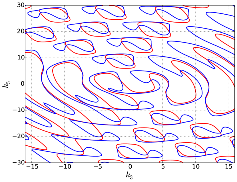
Figure 1: Curves in $(k_{3},k_{5})$ plane formed by optimal values of sine amplitudes. Red curve corresponds to quadratic dependence of ground state amplitude on detuning. Crossing points of red and blue curves correspond to cubic dependence of ground state amplitude on detuning. Such a point nearest to zero is marked by green circle and studied in details. The value of $k_{1}$ is selected so that $\pi$-pulse is formed.

IV.2 Synchronization of the qubits excitation vs detuning

The higher order schemes are build straightforward around the above solution at $N=3$. In this section we collect all the results for $N=1,2,3,4$ order schemes in the driving envelope function (10). In the left column of the fig.2 we plot the optimized shapes of $\pi$-pulses found within the above perturbative approach for a given truncation number $N$. In the right column we show plots illustrating time evolution of qubit excitation dynamics $n_{\uparrow}(t)$ within $\pi$-pulse duration time $0<t<\tau$. Solid curves in the right column in fig.2 correspond to resonant driving $\delta=0$, while dashed ones are related to the detuning $\delta=\Omega$ and $2\Omega$. The dynamics starts from the ground state at $t=0$ and grows significantly at the half of the $\pi$-pulse duration time $\tau/2$. The increase of the $n_{\uparrow}(t)$ resemble the response to singular driving at $t=\tau/2$, because the limit of $f(t)$ at $N\to\infty$ corresponds to ideal $\pi$-pulse with $f_{N\to\infty}(t)=\pi\delta(t-\tau/2)$, which is obviously not achievable experimentally. We stress that we work in the regime of finite $N$ and amplitudes and treat the efficiency of this approach by means of deviation of the resulted $n_{\uparrow}(\tau)$ from unity with respect to non-zero detuning $\delta$. The last two plots in fig.2 illustrate good efficiency of the corresponding $\pi$-pulse shapes: at $N=3$ and $4$ we observe that the dashed curves are very close to the solid ones at $t=\tau$. This means that the inhomogeneous broadening is effectively suppressed in a Rabi frequency range $\propto\Omega$ and this technique offer the synchronization of qubit ensemble starting even from $N=3$.

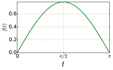
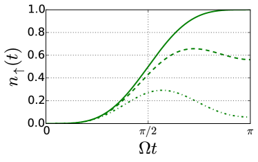
(a)

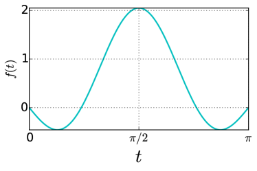
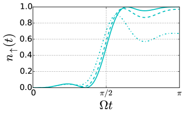
(b)

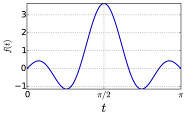
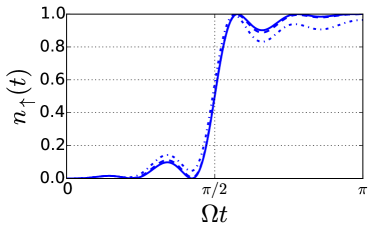
(c)

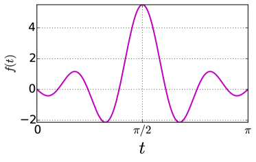
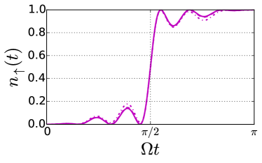
(d)

Figure 2: The shapes of driving amplitudes (on the left) and time dependence of excited level occupation number $n_{\uparrow}(t)$ (on the right) plotted for schemes of a different orders. The driving envelope $f(t)$ shown in fig.2a corresponds to non-optimized $\pi$-pulse and is plotted as a reference.

In the fig.3 we plot numerical results for the dependencies of ground state amplitude absolute values $\sqrt{n_{0}(\tau)}$ after $\pi$-pulse as a function of detuning $\delta$ associated with a spectral broadening. It can be seen that the increase of the scheme order $N$ results in flattening of the curves for $\sqrt{n_{0}(\tau)}$ around point $\delta=0$. This flattening is quantitative demonstration of the inhomogeneous broadening suppression.

The fig.4 is plotted in double logarithmic scale illustrates the precision $n_{0}(\tau)$ of the $\pi$-pulse technique proposed. This figure allows one to estimate the residual value of ground state amplitude for the given scheme order. For instance, for $N=3$ the optimized $\pi$-pulse allows us to achieve the probability of qubit ensemble excitation up to $n_{\uparrow}\approx 1-10^{-3}$ at detuning values up to $\Omega$.

The driving amplitude is limited in real experiment. To illustrate the effect of this limitation we plot the residual ground state amplitude $x(\tau)$ for the pulse of the same shape as mentioned above, but at different $\tau$ so that maximum value of the corresponding envelope does not exceed $\Omega$. These curves are plotted as dashed lines in fig.4.

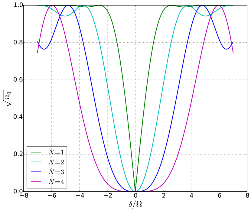
Figure 3: Dependence of ground state amplitude after optimized $\pi$-pulse as a function of detuning in schemes of different orders $N$.

From the curves for $\sqrt{n_{0}(\tau)}$ shown in fig.4 we extract the coefficients of power-law dependencies of residual ground state amplitude for a given $N$. As one can see, the dimensionless combination $n_{0}(\delta)(\delta/\Omega)^{-N}$ does not depend on $\delta$. Dependence on $N$ of logarithmically scaled value of this combination can be fitted by a straight line, as shown in fig.5

$$n_{0}(\delta)=1-n_{\uparrow}\approx 34\left(0.16\frac{\delta}{\Omega}\right)^{2N}$$ (15)

Eq. (15) is one of central results which show quantitative dependence of the precision on the order $N$ and detuning. The small scaling factor $0.16$ for $\delta/\Omega$ shows that this technique based on sine representation (10) could provide the synchronization of ensemble even if the driving signal amplitude is less than a broadening by one order of the magnitude.

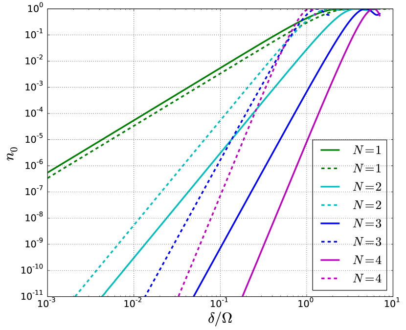
Figure 4: Dependence of residual ground state occupation number after optimized $\pi$-pulse on detuning value plotted in double logarithmic scale. Solid lines correspond to optimized $\pi$-pulses of the same duration $\tau=\pi/\Omega$. Dashed lines correspond to normalized envelopes having maximum absolute value equals to unity. In the latter case the $\pi$-pulse time is not fixed and increases with the increase of scheme order.

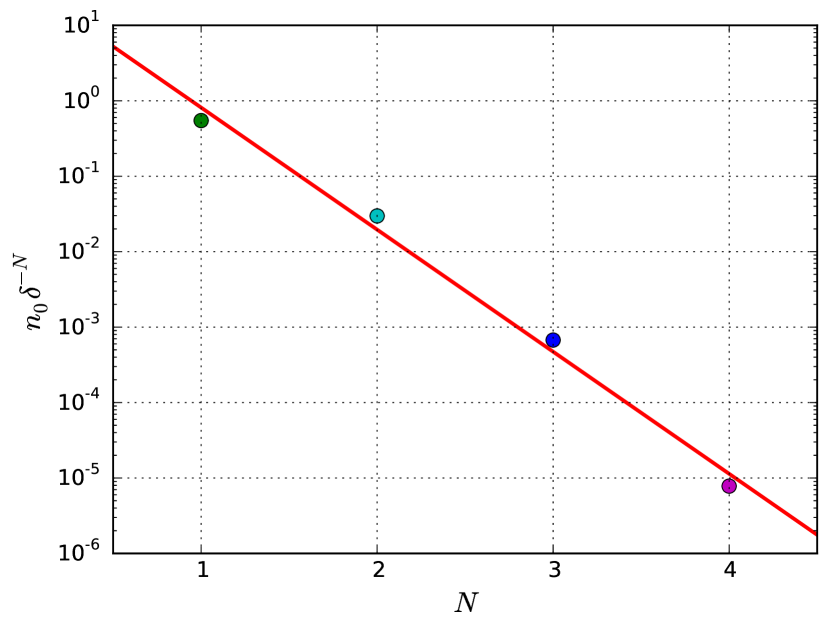
Figure 5: Ground state occupation normalized by appropriate power of detuning after optimized $\pi$-pulse as function of scheme order $N$ involved in $f(t)$.

V Discussion

The efficient excitation of NV-centers in diamond reported in Ref. nv-centers were achieved through the sequences of rectangular pulses with periodical switching of the amplitude sign. This technique demonstrates possibility of excitation of strongly off-resonant qubits by a weak driving signal. We studied an opposite regime when the single non-rectangular $\pi$-pulse effectively suppresses the disorder. The mechanism we are addressed to is related to synchronous excitation dynamics of two level system under a particular non-rectangular envelope shape $f(t)$ of the $\pi$-pulse. We considered non-rectangular smooth shape of the $\pi$-pulse given by external electromagnetic driving $F(0<t<\tau)=f(t)e^{-i\omega t}$ with the envelope representable as the sum of $N$ sine functions $f(t)=\Omega\sum^{N}k_{2n+1}\sin(2n+1)\pi t/(2\tau)$ where the amplitude and pulse duration are locked with each other $\tau=\pi/\Omega$. The off-resonant response of a qubit to a non-rectangular signal can not be calculated exactly and we found the perturbative solution. Within this solution we proposed the method based on optimization of the set of $N$ parameters $k_{2n+1}$ which provide synchronous excitation of the off-resonant qubits. Note, that this optimization is not direct expansion in sine basis of ideal $\pi$-pulse in delta-functional form. The precision of this method, expressed in terms of qubit excitation number $n_{\uparrow}$, is controlled by the order of the scheme and proportional to $(\delta/\Omega)^{2N}$. This scheme is efficient for the qubit energies falling into tunable spectral range estimated as the driving amplitude strength $\Omega$. Within our solution we demonstrated that the $\pi$-pulse formed by $N=4$ sine functions shows simultaneous excitation of qubits with the probability up to $n_{\uparrow}\approx 1-10^{-5}$ for qubit frequencies ranging in $\approx\omega\pm\Omega$.

The sine expansion we used in this approach was based on the experimental requirement of continuity of $f(t)$ at initial and finite moments of time. Optimal envelope shape $f(t)$ can also be found in another basis, say cosine series or rectangular-based blocks. Our calculations shows that in these cases the results will be qualitatively the same as described above. Thus, the proposed method is quite general and can be tuned to meet requirement and restrictions of a particular experiment.

To conclude, we propose the model of smooth shaped single $\pi$-pulse which can be applied to realistic disordered qubit ensembles coupled to a transmission line. Such a $\pi$-pulse provides an effective suppression of the inhomogeneous broadening and can be used as qubit synchronization technique. We expect that our findings could serve as a complementary methods to those reported in Ref.nv-centers , where the sequences of rectangular pulses were used to increase the efficiency in the excitation of qubits within certain frequency range. We also mention that similar technique can be effectively applied to create, say, $\pi/2$-pulse to prepare entangled states of the inhomogeneously broadened qubits.

VI Acknowledgments

Authors thank Alexey V. Ustinov and Walter V. Pogosov for discussions.

References

- (1) A. Blais, R.-S. Huang, A. Wallraff, S. M. Girvin, and R. J. Schoelkopf, Phys. Rev. A 69, 062320 (2004).
- (2) J. Q. You and F. Nori, Nature 474, 589-597 (2011).
- (3) O. Astafiev et al., Science 327, 840 (2010).
- (4) Y. Makhlin, G. Schön, and A. Shnirman, Rev. Mod. Phys. 73, 357-400 (2001).
- (5) J. Clarke and F. K. Wilhelm, Nature 453, 1031-1042 (2008).
- (6) L. DiCarlo et al., Nature 460, 240 (2009).
- (7) P. D. Nation, J. R. Johansson, M. P. Blencowe, and F. Nori, Rev. Mod. Phys. 84, 1 (2012).
- (8) T. P. Orlando, J. E. Mooij, L. Tian, C. H. van der Wal, L. S. Levitov, S. Lloyd, and J. J. Mazo, Phys. Rev. B 60, 15398 (1999).
- (9) J. E. Mooij, T. P. Orlando, L. Levitov, L. Tian, C. H. van der Wal, and S. Lloyd, Science 285, 1036 (1999).
- (10) S. Putz, D. O. Krimer, R. Amsüss, A. Valookaran, T. Nöbauer, J. Schmiedmayer, S. Rotter and J. Majer, Nature Physics 10, 720-724 (2014).
- (11) K. Sandner et al., Phys. Rev. A 85, 053806 (2012).
- (12) M. V. G. Dutt et al., Science 316, 1312 (2007).
- (13) J. J. L. Morton et al., Nature 455, 1085-1088 (2008).
- (14) D. I. Schuster et al., Phys. Rev. Lett. 105, 140501 (2010)
- (15) P. Macha, G. Oelsner, J.-M. Reiner, M. Marthaler, S. André, G. Schön, U. Hübner, H.-G. Meyer, E. Il’ichev, and A.V. Ustinov, Nature Commun. 5, 5146 (2014).
- (16) A. L. Rakhmanov, A. M. Zagoskin, S. Savel’ev, and F. Nori, Phys. Rev. B 77, 144507 (2008).
- (17) P. Volkov and M. V. Fistul, Phys. Rev. B 89, 054507 (2014).
- (18) N. I. Zheludev and Y. S. Kivshar, Nat. Mater. 11, 917-924 (2012).
- (19) D. S. Shapiro, P. Macha, A. N. Rubtsov, and A. V. Ustinov, Photonics 2, 449 (2015).
- (20) T. Brandes, Physics Reports 408, 315 (2005)
- (21) L. J. Zou, D. Marcos, S. Diehl, S. Putz, J. Schmiedmayer, J. Majer, and P. Rabl, Phys. Rev. Lett. 113, 023603 (2014)
- (22) P. L. Stanwix, et al., Phys. Rev. B 82, 201201 (2010).
- (23) J. H. Wesenberg, A. Ardavan, G. A. D. Briggs, J. J. L. Morton, R. J. Schoelkopf, D. I. Schuster, and K. Mølmer, Phys. Rev. Lett. 103, 070502 (2009).
- (24) J. H. Wesenberg, Z. Kurucz, and K. Mølmer, Phys. Rev. A 83, 023826 (2011)
- (25) C. Grezes et al., Phys. Rev. X 4, 021049 (2014).
- (26) H. Wu et al., Phys. Rev. Lett. 105, 140503 (2010).
- (27) B. Julsgaard and K. Mølmer Phys. Rev. A 88, 062324 (2013).
- (28) N. W. Carlson, L. J. Rothberg, A. G. Yodh, W. R. Babbitt, and T. W. Mossberg, Opt. Lett. 8, 483 (1983).
- (29) H. Lin, T. Wang, and T. W. Mossberg, Opt. Lett. 20, 1658 (1995).
- (30) M. Afzelius, C. Simon, H. de Riedmatten, and N. Gisin, Phys. Rev. A 79, 052329 (2009).
- (31) J. S. Hodges et al., Phys. Rev. A 87, 032118 (2013).