Transport across a system with three $p$-wave superconducting wires: effects of Majorana modes and interactions

Abstract

We study the effects of Majorana modes and interactions between electrons on transport in a one-dimensional system with a junction of three $p$-wave superconductors (SCs) which are connected to normal metal leads. For sufficiently long SCs, there are zero energy Majorana modes at the junctions between the SCs and the leads, and, depending on the signs of the $p$-wave pairings in the three SCs, there can also be one or three Majorana modes at the junction of the three SCs. We show that the various sub-gap conductances have peaks occurring at the energies of all these modes; we therefore get a rich pattern of conductance peaks. Next, we use a renormalization group approach to study the scattering matrix of the system at energies far from the SC gap. The fixed points of the renormalization group flows and their stabilities are studied; we find that the scattering matrix at the stable fixed point is highly symmetric even when the microscopic scattering matrix and the interaction strengths are not symmetric. We discuss the implications of this for the conductances. Finally we propose an experimental realization of this system which can produce different signs of the $p$-wave pairings in the different SCs.

1  Introduction

The subject of Majorana fermions has been extensively studied in recent years, both from the fundamental physics point of view beenakker as well as for possible applications in topological quantum computation nayak . A well-studied example of a system which hosts Majorana modes is the Kitaev chain, which is a spin-polarized $p$-wave superconductor (SC) in one dimension. This system is known to have topological phases in which there is a zero energy Majorana mode at each end of a long chain kitaev1 . This system and others similar to it have been theoretically studied in a number of papers beenakker ; lutchyn1 ; fu ; potter ; shivamoggi ; vish ; fidkowski1 ; brouwer ; alicea1 ; fulga ; stanescu1 ; ganga ; stoud ; fidkowski2 ; chung ; sela ; jiang ; dirks ; tewari1 ; beri ; gibertini ; lobos ; hutzen ; pientka1 ; roy ; cook ; sticlet1 ; jose ; klino1 ; alicea2 ; hassler ; sau1 ; liu ; lang ; niu ; degottardi1 ; leijnse ; nadj ; degottardi2 ; cai ; kesel ; klino2 ; adagideli ; mano ; lobos2 ; kashuba ; ghaza ; guigou ; klino3 ; door ; kao ; hegde ; thakurathi ; spanslatt ; dasmandal . Several experiments inspired by these models have looked for Majorana modes, either through a zero bias conductance peak kouwenhoven ; deng ; das1 ; finck ; lee ; nadj2 ; pawlak or through the fractional Josephson effect rokhinson . The zero bias peak occurs because the Majorana mode (which lies at zero energy for a long enough system) allows an electron to tunnel from a normal metal lead into the superconductor where it turns into a Cooper pair; this gives rise to a perfect Andreev reflection back into the lead.

The Kitaev chain has been generalized in a number of ways; some of these generalizations give rise to more than one Majorana mode at each end of the SC region fidkowski1 ; potter ; beri ; niu ; degottardi2 . The case of additional Majorana modes appearing inside the bulk of the SC region (rather than at the ends) is less well studied. Strictly speaking, the term Majorana modes is used to refer to states with exactly zero energy. In this paper, we will discuss various sub-gap modes which lie within the SC gap but may or may not lie at zero energy. All these modes originate from the zero energy Majorana modes which occur if the SC wires are very long, but they hybridize and thereby move away from zero energy when the wire lengths are finite. It is interesting to study the effect of all such sub-gap modes on the electronic transport across the system.

The effect of interactions between the electrons is also of interest. In one dimension, interactions are known to have a dramatic effect, turning the system into a Tomonaga-Luttinger liquid. The fate of the Majorana modes in the presence of interactions has been studied extensively ganga ; sela ; lobos ; hutzen ; hassler ; stoud ; fidkowski2 ; mano ; kashuba ; ghaza . We will examine a different aspect of our system, namely, the fixed points of the conductances which arise from the renormalization group flows induced by interactions.

In this paper, we will study the conductances of a one-dimensional system consisting of a junction of three finite-sized $p$-wave superconductors, each of which is in turn connected to a semi-infinite normal metal (NM) lead. We will study transport in two different regimes of the energy, namely, inside the SC gap and far outside the gap.

In the first part of this paper, we will study the Majorana and related sub-gap modes and their effect on the sub-gap conductances. A motivation for studying a junction of three $p$-wave superconductors is that a topological quantum computation using Majorana modes in quasi-one-dimensional systems would involve braiding of two Majorana modes without the two modes ever coming close to each other. In order to achieve this we must consider junctions of three or more wires, so that a Majorana mode can be moved from the first wire to the second without disturbing a Majorana mode lying on the third wire. (A single superconducting wire does not allow braiding of Majorana modes). We will show that there are two interesting possibilities for a junction of three superconducting wires which have rather different properties: the $p$-wave pairing amplitude $\Delta$ can have the same sign in all three SCs, or $\Delta$ can have the same sign in two of the SCs and the opposite sign in the third SC. We will see that the number of zero energy Majorana modes is different in the two cases when the SC wires are very long (namely, much longer than the decay length which will be discussed below). In the first case, there are six Majorana modes (three at the NM-SC junctions, and three more at the junction of the three SCs), while in the second case, there are four Majorana modes (three at the NM-SC junctions and only one at the junction of the SCs). The fact that there can be three Majorana modes at a junction of three $p$-wave superconducting wires has not been pointed out earlier as far as we know.

We would like to note that many kinds of junctions have been studied before, such as junctions of three wires or three spin-1/2 chains (which can be mapped to fermionic chains) alicea1 ; zhou ; tsvelik , a superconducting junction of non-superconducting wires erik ; alt , and a junction of multiple non-superconducting wires with a superconducting wire affleck . In this paper, we will not consider the effect of interactions at the junction (i.e., charging energy) which leads to the Kondo-Majorana physics studied in Refs. erik, and alt, . However we will discuss the effect of interactions in the wires away from the junction as mentioned below.

Electronic transport across a NM-SC-NM system has been studied for many years blonder ; kasta ; ks01 ; yoko ; hayat . The presence of a SC means that there will be both normal reflection and transmission and Andreev reflection and transmission blonder ; andreev . Hence there are two kinds of differential conductances which can be measured in this NSN system: a conductance from one NM lead to the other NM lead which we will call $G_{N}$, and a Cooper pair conductance from a NM lead to the SC which we will call $G_{C}$. In our system with three SCs and three NM leads, we will consider an electron incident from one of the leads (called NM1); we can then have a conductance $G_{C}$ from that lead to the SC, and conductances $G_{N2}$ and $G_{N3}$ from that lead to the other two leads called NM2 and NM3 respectively. We will use a continuum model for this system, rather than the Kitaev model which is defined on a lattice. We will first present the boundary conditions at the three NM-SC junctions which follow from the conservation of both the probability and charge currents. We will then discuss the boundary conditions at the junction of the three SCs; this will turn out to involve a $3\times 3$ Hermitian matrix $\bf M$ which determines how a current incident on the junction from one of the SCs either gets reflected back to that SC or gets transmitted to the other two SCs. Using all these boundary conditions, we will numerically calculate $G_{C},~{}G_{N2}$ and $G_{N3}$ as functions of the energy $E$ of the electron incident from the lead NM1 and the lengths $L_{j}$ of the three SCs. We will see that $G_{C}$ has a rich structure of peaks when $E$ lies in the superconducting gap. The conductance calculation will be followed by the discussion of a box made of only the SCs with hard wall boundary conditions (namely, with no NM leads). We will numerically calculate the energies of the sub-gap modes in this system and show that this explains the locations of the peaks in the conductance $G_{C}$ of the system with NM leads.

In the second part of the paper, we will study the effect of interactions between the electrons on the conductances of the system at energies which are far from the SC gap, namely, when $|E|\gg|\Delta|$. (The Majorana and other sub-gap modes play no role in this part; this is therefore complementary to the first part of the paper where we look at the sub-gap conductances). It is common to use the technique of bosonization to study one-dimensional systems with interacting electrons gogolin . However, for reasons that will be discussed below, it turns out to be difficult to use bosonization when there is a junction of three or more wires and superconductivity is present. (Three-wire junctions without superconductivity have been studied in Refs. nayak2, ; trau, ; chamon, ; bella, ; agar, using bosonization and in Ref. meden, using functional renormalization group methods. Junctions between a superconducting wire and multiple non-superconducting wires with interactions have been studied using bosonization affleck ). We will therefore use a different method which is valid when the strength of the interactions is weak yue ; lal ; das2 ; saha . Using this method we will find that the scattering matrix $S$ which characterizes the junction of three wires effectively becomes a function of the length scale, and we will find a renormalization group (RG) equation for $S$. Using the RG equation, we will study how $S$ varies with the length scale; we will find the fixed points of the RG equation and study their stabilities. We will then discuss the implications of this for the conductances of the system when the wire lengths are large or the temperature is low.

The plan of the paper is as follows. In Sect. 2, we introduce the model for the NSN system and derive the boundary conditions at the junctions between the SCs and the NM leads and at the junction of three SCs. We show how this can be used to derive the various differential conductances $G_{Nj}$ and $G_{C}$ at energies lying inside the SC gap. In Sect. 3, we numerically calculate $G_{Nj}$ and $G_{C}$ for two cases: when the $p$-wave pairings $\Delta_{j}$ have the same sign in all the three wires and when one of them has a different sign from the other two. We discuss three different regimes of the lengths of the SC wires: these lengths can be less than, a little larger than, and much larger than the decay length of the sub-gap modes which appear near the different junctions. The locations of the peaks in the conductances are quite different in the three length regimes and also in the two cases of the relative signs of the $\Delta_{j}$. To understand these differences, we have numerically found the energies of the sub-gap modes and shown that they precisely match the locations of the conductance peaks. In Sect. 4, we provide analytical arguments to show that the number of zero energy Majorana modes at the junction of three long $p$-wave SCs is three if the $\Delta_{j}$’s have the same sign but is one if one of the $\Delta_{j}$’s has a different sign. In Sect. 5, we study the effect of interactions between the electrons on the conductance at energies far from the SC gap (but much smaller than the band width of the system). To this end we consider a junction of three NM wires which meet in a SC region, and we derive the RG equations for the scattering matrix of this system for the case where the electrons interact weakly with each other. In Sect. 6, we study the fixed points and stabilities of the RG equations and show that this can lead to power-law dependences of the conductances on the wire lengths or temperature. In Sect. 7 we show how a system of three $p$-wave SCs can be experimentally realized and how the two cases of all the $\Delta_{j}$’s having the same sign or one of them having a different sign can be fabricated. We end in Sect. 8 with a summary of our results.

2  Model for a system of three SC wires making a $Y$-junction

We begin with a continuum model for a $Y$-junction of three $p$-wave SC wires in one dimension as shown in Fig. 1. A NM lead is attached to the end of each SC where there is a barrier modeled by a $\delta$-function potential. Each NM-SC system has a coordinate system $x_{j}$, with $j=1,2,3$; we define the point where the three SCs meet as the origin $x_{j}=0$ for all $j$. As we move away from this junction, $x_{j}$ will be taken to increase. The different SCs may have different lengths and lie in the regions $0\leq x_{j}\leq L_{j}$; the leads lie in the region $L_{j}\leq x_{j}<\infty$.

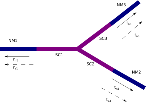
Figure 1: Schematic picture of a $Y$-junction of three wires labeled as 1-3. The inner (lighter) regions of the wires are $p$-wave SCs while the outer (darker) regions are NM leads. For an electron incident from NM1, six amplitudes are shown in the leads: $r_{n1},~{}r_{a1}$ are normal and Andreev reflections in NM1, $t_{n2},~{}t_{a2}$ are normal and Andreev transmissions in NM2, and $t_{n3},~{}t_{a3}$ are normal and Andreev transmissions in NM3.

Let us denote the wave function in wire $j$ as $\psi=(c,~{}d)^{T}$, where $c(x_{j},t),~{}d(x_{j},t)$ are the electron and hole components respectively (we assume that the electrons are spin-polarized and will therefore ignore the spin label). The Hamiltonian in each wire can be written as

$$H = \int_{0}^{\infty}dx_{j}~{}[c^{\dagger}(-\frac{\hbar^{2}\partial_{x_{j}}^{2}}{2m}-\mu)c~{}-~{}d^{\dagger}(-\frac{\hbar^{2}\partial_{x_{j}}^{2}}{2m}-\mu)d$$ (1)

$$~{}~{}~{}~{}~{}~{}~{}~{}~{}-\frac{i\Delta_{j}}{k_{F}}~{}(c^{\dagger}\partial_{x_{j}}d+d^{\dagger}\partial_{x_{j}}c)],$$

where $\mu$ is the chemical potential, $k_{F}=\sqrt{2m\mu}/\hbar$ is the Fermi wave number, and $\Delta_{j}$ is the $p$-wave superconducting pairing amplitude which will be assumed to be real everywhere; we will set $\Delta_{j}=0$ in the NM leads. (We will generally set $\hbar=1$ in this paper, except in places where it is required for clarity). The Heisenberg equations of motion $i\partial_{t}c=-[H,c]$ and $i\partial_{t}d=-[H,d]$ imply that

$$i\partial_{t}c = -\left(\frac{\partial_{x_{j}}^{2}}{2m}+\mu\right)~{}c~{}-~{}\frac{i\Delta_{j}}{k_{F}}~{}\partial_{x_{j}}d,$$

$$i\partial_{t}d = \left(\frac{\partial_{x_{j}}^{2}}{2m}+\mu\right)~{}d~{}-~{}\frac{i\Delta_{j}}{k_{F}}~{}\partial_{x_{j}}c.$$ (2)

For a wave function which varies in space as $e^{\pm ikx_{j}}$, the energy is given by $\pm[k^{2}/(2m)-\mu]$ if $\Delta_{j}=0$, and by $\pm\sqrt{[k^{2}/(2m)-\mu]^{2}+\Delta_{j}^{2}(k/k_{F})^{2}}$ if $\Delta_{j}\neq 0$. The corresponding wave functions will be presented below. We see that the energy spectrum in the $j$-th SC has a gap equal to $2\Delta_{j}$ at $k=\pm k_{F}$.

Let us define the particle density $\rho_{p}=c^{\dagger}c+d^{\dagger}d$ (this counts electrons and holes with the same sign) and the charge density $\rho_{c}=c^{\dagger}c-d^{\dagger}d$ (which counts electrons and holes with opposite signs; we are ignoring a factor of electron charge here). Using Eqs. (2) and the equations of continuity $\partial_{t}{\rho_{p}}+\partial_{x}J_{p}=0$ and $\partial_{t}{\rho_{c}}+\partial_{x}J_{c}=0$, we find the particle and charge currents to be blonder ; soori

$$J_{p} = \frac{i}{2m}~{}[-~{}c^{\dagger}\partial_{x}c~{}+~{}\partial_{x}c^{\dagger}c~{}+~{}d^{\dagger}\partial_{x}d~{}-~{}\partial_{x}d^{\dagger}d]$$

$$+~{}\frac{\Delta}{k_{F}}~{}(c^{\dagger}d+d^{\dagger}c),$$

$$J_{c} = J_{1}~{}+~{}\int_{0}^{x}dx^{\prime}~{}J_{2}(x^{\prime}),$$

$$J_{1} = \frac{i}{2m}~{}[-~{}c^{\dagger}\partial_{x}c~{}+~{}\partial_{x}c^{\dagger}c~{}-~{}d^{\dagger}\partial_{x}d~{}+~{}\partial_{x}d^{\dagger}d],$$

$$J_{2} = -~{}\frac{2\Delta}{k_{F}}~{}(\partial_{x}c^{\dagger}d+d^{\dagger}\partial_{x}c).$$ (3)

The last term, $J_{2}$, can be interpreted as the contribution of Cooper pairs to the charge current; note that it vanishes in the NM where $\Delta=0$.

The boundary conditions at the NM-SC junctions at $x_{j}=L_{j}$ can be found by demanding that the currents $J_{p}$ and $J_{c}$ be conserved at those points. At the junction $x_{1}=L_{1}$, let us consider the wave functions $\psi_{nm1}=(c_{nm1},~{}d_{nm1})^{T}$ and $\psi_{sc1}=(c_{sc1},~{}d_{sc1})^{T}$ at the points $x_{1}=L_{1}+\epsilon$ and $x_{1}=L_{1}-\epsilon$, i.e., in the NM and SC regions respectively. The condition $J_{p}(L_{1}+\epsilon)=J_{p}(L_{1}-\epsilon)$ implies that

$$\frac{i}{2m}~{}[-~{}c_{nm1}^{\dagger}\partial_{x_{1}}c_{nm1}~{}+~{}\partial_{x_{1}}c_{nm1}^{\dagger}c_{nm1}$$ (4)

$$~{}~{}~{}~{}~{}~{}+~{}d_{nm1}^{\dagger}\partial_{x_{1}}d_{nm1}~{}-~{}\partial_{x_{1}}d_{nm1}^{\dagger}d_{nm1}]$$

$$= \frac{i}{2m}~{}[-~{}c_{sc1}^{\dagger}\partial_{x_{1}}c_{sc1}~{}+~{}\partial_{x_{1}}c_{sc1}^{\dagger}c_{sc1}$$

$$~{}~{}~{}~{}~{}~{}+~{}d_{sc1}^{\dagger}\partial_{x_{1}}d_{sc1}~{}-~{}\partial_{x_{1}}d_{sc1}^{\dagger}d_{sc1}]$$

$$~{}+~{}\frac{\Delta_{1}}{k_{F}}~{}(c_{sc1}^{\dagger}d_{sc1}~{}+~{}d_{sc1}^{\dagger}c_{sc1}).$$

The simplest way of satisfying this condition is to set

$$c_{sc1} = c_{nm1},$$

$$d_{sc1} = d_{nm1},$$

$$\partial_{x_{1}}c_{sc1}~{}+~{}\frac{i\Delta_{1}}{v_{F}}~{}d_{sc1} = \partial_{x_{1}}c_{nm1},$$

$$\partial_{x_{1}}d_{sc1}~{}-~{}\frac{i\Delta_{1}}{v_{F}}~{}c_{sc1} = \partial_{x_{1}}d_{nm1},$$ (5)

where $v_{F}=k_{F}/m$ is the Fermi velocity. The first two equations above mean that the wave function is continuous while the last two equations imply that the first derivative is discontinuous in a particular way. We now find that Eqs. (5) imply that the charge current is conserved, namely, $J_{c}(L_{1}-\epsilon)=J_{c}(L_{1}+\epsilon)$. Next, let us consider what happens if a $\delta$-function potential of strength $\lambda$ is present at the junction at $x_{1}=L_{1}$; note that the dimension of $\lambda$ is energy times length. (This potential is physically motivated by the fact that in many experiments, the NM leads are weakly coupled, by a tunnel barrier, to the SC. This can be modeled by placing a $\delta$-function potential with a large strength at the junction). Now there will be an additional discontinuity in the first derivative at $x_{1}=L_{1}$; this is found by integrating over the $\delta$-function which gives

$$\partial_{x_{1}}\psi_{nm1}(L_{1}+\epsilon)~{}-~{}\partial_{x_{1}}\psi_{sc1}(L_{1}-\epsilon)~{}=~{}2m\lambda~{}\psi_{nm1}(0).$$ (6)

Hence Eqs. (5) must be modified to

$$c_{sc1} = c_{nm1},$$

$$d_{sc1} = d_{nm1},$$

$$\partial_{x_{1}}c_{sc1}~{}+~{}\frac{i\Delta_{1}}{v_{F}}~{}d_{sc1}~{}+~{}2m\lambda~{}c_{sc1} = \partial_{x_{1}}c_{nm1},$$

$$\partial_{x_{1}}d_{sc1}~{}-~{}\frac{i\Delta_{1}}{v_{F}}~{}c_{sc1}~{}+~{}2m\lambda~{}d_{sc1} = \partial_{x_{1}}d_{nm1}.$$ (7)

For the other two NM-SC junctions at $x_{2}=L_{2}$ and $x_{3}=L_{3}$, we will get boundary conditions similar to Eqs. (7).

We have found the boundary conditions at the NM-SC junctions. Now we look at the junction $x_{j}=0$ where the three SCs meet. We can find the boundary conditions at this junction using the conservation of the particle current $J_{p}$; this implies that

$$\sum_{j}{J_{p_{j}}} = \frac{i}{2m}~{}\sum_{j}{[-~{}c_{scj}^{\dagger}\partial_{x_{j}}c_{scj}~{}+~{}\partial_{x_{j}}c_{scj}^{\dagger}c_{scj}]}$$ (8)

$$+~{}\frac{i}{2m}~{}\sum_{j}{[d_{scj}^{\dagger}\partial_{x_{j}}d_{scj}~{}-~{}\partial_{x_{j}}d_{scj}^{\dagger}d_{scj}]}$$

$$+~{}\sum_{j}{\frac{\Delta_{j}}{k_{F}}~{}(c_{scj}^{\dagger}d_{scj}+d_{scj}^{\dagger}c_{scj})}$$

$$= 0.$$

The simplest way of satisfying this condition is to set

$$\partial_{x}c_{sc} = {\bf M}\cdot c_{sc}~{}+~{}{\bf N}\cdot d_{sc},$$

$$\partial_{x}d_{sc} = {\bf M^{*}}\cdot d_{sc}~{}+~{}{\bf N^{*}}\cdot c_{sc},$$ (9)

where $c_{sc}\equiv(c_{sc1},c_{sc2},c_{sc3})^{T}$, $d_{sc}\equiv(d_{sc1},d_{sc2},d_{sc3})^{T}$, and ${\bf M},~{}{\bf N}$ are $3\times 3$ matrices. Substituting the above conditions in Eq. (8), we find that we must have

$${\bf M}^{\dagger} = {\bf M},$$

$${\bf N}~{}+~{}{\bf N^{T}} = -\frac{i2m}{k_{F}}~{}{\bf\Delta},$$ (10)

where ${\bf\Delta}=\left(\begin{array}[]{ccc}\Delta_{1}&0&0\\ 0&\Delta_{2}&0\\ 0&0&\Delta_{3}\end{array}\right)$. In our calculations we will assume that the magnitudes of all the $\Delta_{j}$’s are the same but the signs of $\Delta_{j}$ may vary with $j$. Now we will use the conservation of the charge current $J_{c}$ at the junction $x_{j}=0$. The second term in the expression in Eq. (3) for the charge current, namely, $\int_{0}^{x_{j}}dx^{\prime}~{}J_{2}(x^{\prime})$ goes to zero as $x_{j}\to 0$. So the conservation of $J_{c}$ implies that

$$\sum_{j}{J_{c_{j}}} = \frac{i}{2m}~{}\sum_{j}{[-~{}c_{scj}^{\dagger}\partial_{x_{j}}c_{scj}~{}+~{}\partial_{x_{j}}c_{scj}^{\dagger}c_{scj}]}$$ (11)

$$~{}+~{}\frac{i}{2m}~{}\sum_{j}{[-d_{scj}^{\dagger}\partial_{x_{j}}d_{scj}+\partial_{x_{j}}d_{scj}^{\dagger}d_{scj}]}$$

$$= 0.$$

Using Eq. (9) in the above expression we find that

$${\bf N}~{}=~{}-~{}\frac{im}{k_{F}}~{}{\bf\Delta}.$$ (12)

Hence Eq. (9) becomes

$$\partial_{x}c_{sc} = {\bf M}\cdot c_{sc}~{}-~{}\frac{im}{k_{F}}~{}{\bf\Delta}\cdot d_{sc},$$

$$\partial_{x}d_{sc} = {\bf M^{*}}\cdot d_{sc}~{}+~{}\frac{im}{k_{F}}~{}{\bf\Delta}\cdot c_{sc}.$$ (13)

It is useful to note some symmetries of our system.

(i) Eqs. (2) are symmetric under time reversal (which changes $t\to-t$ and complex conjugates all numbers) if we transform $c\to c^{*}$ and $d\to-d^{*}$. This will also be a symmetry of Eqs. (13) if ${\bf M^{*}}={\bf M}$. Eq. (10) then implies that ${\bf M}$ must be both real and symmetric. We will assume this henceforth.

(ii) Eqs. (2), (7) and (13) remain invariant under the transformation

$$c(x_{j}) \to i~{}c(x_{j}),~{}~{}~{}~{}d(x_{j})~{}\to~{}-i~{}d(x_{j}),$$

$$\Delta_{j} \to -~{}\Delta_{j},$$ (14)

for all value of $j$ and $x_{j}$. This implies that the conductances discussed below remain invariant if $\Delta_{j}\to-\Delta_{j}$ on all the wires.

We now use the boundary conditions discussed above to find the various reflection and transmission amplitudes when an electron is incident from, say, the NM1 lead with unit amplitude. In the presence of the SCs, the various scattering processes that may occur are as follows blonder .

(i) an electron can be reflected back to the NM1 lead with amplitude $r_{n1}$.

(ii) a hole can be reflected back to the NM1 lead with amplitude $r_{a1}$. Charge conservation then implies that a Cooper pair must be produced inside the region SC1.

(iii) an electron can be transmitted to the NM2 lead with amplitude $t_{n2}$.

(iv) a hole can be transmitted to the NM2 lead with amplitude $t_{a2}$. (This is usually called crossed Andreev reflection law2 ). Then charge conservation implies that a Cooper pair must be produced inside SC2.

(v) an electron can be transmitted to the NM3 lead with amplitude $t_{n3}$.

(vi) a hole can be transmitted to the NM3 lead with amplitude $t_{a3}$ which implies that a Cooper pair must be produced inside SC3.

If the energy $E$ of the electron (incident from the lead NM1) lies in the superconducting gap, i.e., $-\Delta\leq E\leq\Delta$ ($E$ can be interpreted as the bias between the chemical potentials of NM1 and the SCs), Eqs. (2) imply that the wave functions in the different regions must be of the form

$$\psi_{nm1} = e^{-i(k_{F}+k)x_{1}}~{}\left(\begin{array}[]{c}1\\ 0\end{array}\right)+~{}r_{n1}~{}e^{i(k_{F}+k)x_{1}}~{}\left(\begin{array}[]{c}1\\ 0\end{array}\right)$$ (22)

$$+~{}r_{a1}~{}e^{i(-k_{F}+k)x_{1}}~{}\left(\begin{array}[]{c}0\\ 1\end{array}\right),$$

$$\psi_{nm2} = t_{n2}~{}e^{i(k_{F}+k)x_{2}}~{}\left(\begin{array}[]{c}1\\ 0\end{array}\right)+~{}t_{a2}~{}e^{i(-k_{F}+k)x_{2}}~{}\left(\begin{array}[]{c}0\\ 1\end{array}\right),$$ (27)

$$\psi_{nm3} = t_{n3}~{}e^{i(k_{F}+k)x_{3}}~{}\left(\begin{array}[]{c}1\\ 0\end{array}\right)+~{}t_{a3}~{}e^{i(-k_{F}+k)x_{3}}~{}\left(\begin{array}[]{c}0\\ 1\end{array}\right),$$ (32)

$$\psi_{scj} = t_{1j}~{}e^{ik_{1}x_{j}}~{}\left(\begin{array}[]{c}1\\ sgn(\Delta_{j})~{}e^{i\phi}\end{array}\right)$$ (44)

$$+~{}t_{2j}~{}e^{-ik_{2}x_{j}}~{}\left(\begin{array}[]{c}1\\ -sgn(\Delta_{j})~{}e^{-i\phi}\end{array}\right)$$

$$+~{}t_{3j}~{}e^{ik_{3}x_{j}}~{}\left(\begin{array}[]{c}1\\ sgn(\Delta_{j})~{}e^{-i\phi}\end{array}\right)$$

$$+~{}t_{4j}~{}e^{-ik_{4}x_{j}}~{}\left(\begin{array}[]{c}1\\ -sgn(\Delta_{j})~{}e^{i\phi}\end{array}\right),$$

where $e^{i\phi}=(E-i\sqrt{\Delta^{2}-E^{2}})/\Delta$, and $sgn$ denotes the sign function. (We have assumed that the magnitudes of the $\Delta_{j}$ are the same; hence $e^{i\phi}$ is the same for the three SCs). The top and bottom entries in the wave functions denote the particle and hole components. The wave functions in the NM leads are proportional to $e^{i(\pm k_{F}+k)x_{j}}$, where $k\ll k_{F}$, namely, we are working close to the Fermi energy. In each SC, we have four modes; two of these decay exponentially while the other two grow as we move away from the junction of the three SCs. We denote the wave numbers of these modes by $k_{1},~{}-k_{2},~{}k_{3}$ and $-k_{4}$. Defining the decay length

$$\xi~{}=~{}\frac{v_{F}}{\Delta\sqrt{1-(E/\Delta)^{2}}},$$ (45)

we find that the decaying modes have

$$k_{1} = k_{F}+i/\xi,$$

$$-k_{2} = -k_{F}+i/\xi,$$ (46)

while the growing modes have

$$k_{3} = k_{F}-i/\xi,$$

$$\ -k_{4} = -k_{F}-i/\xi.$$ (47)

From Eqs. (7) we get the relation between the wave functions on the NM and SC sides at each of the NM-SC junctions. Similarly, from Eqs. (10) and (12) we get the relation among the wave functions of the three SCs at the junction where they meet. We thus have eighteen equations for the eighteen unknowns $r_{n1},~{}r_{a1},~{}t_{n2},~{}t_{a2},~{}t_{n3},~{}t_{a3},~{}t_{1j},~{}t_{2j},~{}t_{3j}$ and $t_{4j}$, where $j=1,2,3$. After solving these equations we can calculate the reflection and transmission probabilities. The conservation law for the probability current implies that

$$|r_{n1}|^{2}~{}+~{}|r_{a1}|^{2}~{}+~{}|t_{n2}|^{2}~{}+~{}|t_{a2}|^{2}~{}+~{}|t_{n3}|^{2}~{}+~{}|t_{a3}|^{2}~{}=~{}1.$$ (48)

The net probabilities for an electron to be transmitted from the NM1 lead to the NM2 and NM3 leads gives the differential conductances $G_{N2}$ and $G_{N3}$ respectively, where

$$G_{N2} = |t_{n2}|^{2}~{}-~{}|t_{a2}|^{2},$$

$$G_{N3} = |t_{n3}|^{2}~{}-~{}|t_{a3}|^{2}.$$ (49)

The net probability for the electron to be reflected back to the NM1 lead is

$$G_{B}~{}=~{}|r_{n1}|^{2}~{}-~{}|r_{a1}|^{2}.$$ (50)

The remainder, denoted by the differential conductance $G_{C}$, is the probability for the electron to be transmitted into the SCs in the form of Cooper pairs. The conservation of charge current implies that

$$G_{C} = 1~{}-~{}G_{N2}~{}-~{}G_{N3}~{}-~{}G_{B}$$ (51)

$$= 2~{}(|r_{a1}|^{2}~{}+~{}|t_{a2}|^{2}~{}+~{}|t_{a3}|^{2}),$$

where we have used Eqs. (48-50) to derive the last line in Eq. (51). [Actually, the differential conductances into the NM leads 2 and 3 and into the SCs are given by $e^{2}/(2\pi\hbar)$ times $G_{N2}$, $G_{N3}$ and $G_{C}$ respectively, where $e$ is the charge of an electron. However, we will ignore the factors of $e^{2}/(2\pi\hbar)$ in this paper and simply refer to $G_{Nj}$ and $G_{C}$ as the differential conductances.]

We note that a differential conductance denotes $G=dI/dV$. To measure $G_{N2}$, $G_{N3}$ and $G_{C}$ in our system, we have to assume that there is a voltage bias $V$ between the NM1 lead on the one hand and the SCs and the NM leads on the other (the SCs, NM2 and NM3 are taken to be at the same potential). Namely, we choose the mid-gap energy in the SCs as zero, and the Fermi energies in the NM1 lead as $E=eV$ and in NM2 and NM3 as zero. The differential conductances $G_{Nj}=dI_{Nj}/dV$ and $G_{C}=dI_{C}/dV$ are then the derivatives with respect to $V$ of the currents measured in the NM leads and in the SCs.

3  Numerical results

3.1  All $\Delta_{j}$’s with the same sign

In this section we present numerical results for $G_{C}$ and $G_{N2}$ as functions of the length $L_{1}$ of SC1 and the ratio $E/\Delta$ lying in the range $[-1,1]$. The length scale associated with the SC gap is $\eta=v_{F}/\Delta=k_{F}/{m\Delta}$. (This is different from the length $\xi$ introduced in Eq. (45) which depends on the energy $E$. Note that $\xi=\eta$ if $E=0$). We study three cases, namely, $L<\eta$, $L\sim\eta$ and $L>\eta$.

The values of the parameters that we have used to numerically calculate the conductances are as follows: $k_{F}=1$, $m=0.5$, $\lambda=5$, and $\Delta_{1}=\Delta_{2}=\Delta_{3}=\Delta=0.1$. Throughout this section and in the next, we will take the matrix at the junction of the three SC wires to be of a form which is completely symmetric under any permutation of the three wires,
${\bf M}=\left(\begin{array}[]{ccc}1&1&1\\ 1&1&1\\ 1&1&1\end{array}\right)$.
The diagonal terms of ${\bf M}$ connect $\partial_{x}c~{}(\partial_{x}d)$ and $c~{}(d)$ in the same wire, while the off-diagonal terms connect $\partial_{x}c~{}(\partial_{x}d)$ and $c~{}(d)$ in different wires. If we choose the off-diagonal and diagonal elements of ${\bf M}$ to be different, some of the results for the conductances may differ from what we will discuss below.

In the first row of Fig. 2, we have shown top views of $G_{C}$. In the third row we show surface plots of $G_{N2}$ which is the conductance in NM2. In our calculations we have chosen $L_{2}$ and $L_{3}$ not to differ much from each other, so that $G_{N2}$ and $G_{N3}$ are similar. Hence we have presented $G_{N2}$ only.

To understand the conductance plots better we consider another system which is made of three SC wires but is not connected to any NM leads; namely, there is an infinite barrier at the ends of the SC wires. Thus this system is similar to a particle in a box but the box is made of three SC wires. The wave function is zero at the ends of the wires because of the infinite barriers present there. At the junction of the three wires we use the same boundary condition that we derived in Eqs. (13). Using the boundary conditions we get a set of twelve linear homogeneous equations for the amplitudes $t_{1j},~{}t_{2j},~{}t_{3j}$ and $t_{4j}$ in the SC wires. These equations have a non-trivial solution if the determinant $D$ of the matrix constructed from these equations is zero. We plot the determinant $D$ as a function of $L_{1}$ and $E/\Delta$. The points where $D=0$ give the parameter values where sub-gap modes appear in the system. In the second row of Fig. 2, we have shown the top views of $D$; the lightest regions correspond to the points closest to $D=0$. We expect that the positions of the peaks of $G_{C}$ will match the positions of the zeros of $D$ as $L_{1}$ and $E/\Delta$ are varied.

For the parameter values we have chosen, we find that $\eta=20$. In the first column of Fig. 2, we take $L_{1}=3.5\pi$ to $7.5\pi$ (so that $L_{1}<\eta$), $L_{2}=6.7\pi$ and $L_{3}=6.3\pi$. In this regime we find that there are six sub-gap modes inside the SCs which is evident from the top view of $G_{C}$ in Fig. 2 (a). If we look at a particular value of $L_{1}$ in that figure, we see six different modes at different energies. (Some of the modes look fainter than the others). Three of the sub-gap modes lie near the NM-SC junctions as we know from earlier papers (see, for example, Ref. thakurathi, ). The other three modes must lie near the three-wire junction. To explain the presence of modes at non-zero energies, we recall that the momenta in the SC have an imaginary part, giving rise to factors of $\pm x_{j}/\xi$ as we can see from the expression for $\psi_{scj}$ in Eq. (44). On wire $j$, the sub-gap wave functions of the form $e^{x_{j}/\xi}$ decay exponentially as we go away from the NM-SC junction, while the wave functions of the form $e^{-x_{j}/\xi}$ decay as we go away from the junction of three SC wires. When the lengths of the SCs are small compared to the decay length $\xi$ of the sub-gap modes, the amount of decay of the modes inside the SC will be small. Hence, the sub-gap modes at the NM-SC junctions and at the junction of three SC wires will hybridize and their energies will split from zero. So the mixing of the sub-gap modes for SC wires with small lengths is responsible for the appearance of states at non-zero energies. These energies oscillate with $L_{1}$ and vanish at certain values of $L_{1}$.

As there are states inside the SCs and the lengths of the SCs are smaller than the decay length $\xi$, there are two possibilities for an electron coming from the lead NM1.

(i) It can enter the SC1 by coupling to the Majorana mode sitting there and then turn into a Cooper pair; a hole goes back into NM1 to conserve charge. In this process we get a finite $r_{a1}$ and hence a finite $G_{C}$.

(ii) It can enter the SC1 similarly as described above and can then get transmitted to the other two NMs as the wave functions of the sub-gap modes decay very little inside the SCs. So we get finite transmission probabilities and hence a finite $G_{N2}$ and $G_{N3}$. From the figures in the first column of Fig. 2, it is clear that both $G_{C}$ and $G_{N2}$ are appreciable when $L_{1}<\eta$.

In the third column of Fig. 2, we choose $L_{1}=70.5\pi$ to $74.5\pi$, $L_{2}=68.3\pi$ and $L_{3}=68.7\pi$, so that all the lengths are much larger than the decay length $\xi$ of the sub-gap modes. In this regime the sub-gap modes are mostly localized at the ends of the SCs and at the junction of the three SC wires. So the coupling between the different sub-gap modes are small, and their energies remain almost at zero. In Figs. 2 (c) and (i), we see that instead of six sub-gap modes at different energies, we now have all the sub-gap modes near zero energy (namely, they are almost Majorana modes). There is a small splitting in the energy around $E=0$ because of a small non-zero coupling between the different modes. If we increase the various lengths more, we expect to see no splitting at all and all the modes should stay exactly at $E=0$.

In the large length regime we find that $G_{C}$ almost approaches its highest value of 2 (in units of $e^{2}/h$) while $G_{N2}$ is very small. The reason for this is that the sub-gap modes are now almost decoupled from each other; due to the exponential decay of their wave functions, the probability of an electron to travel through the SCs and get transmitted to the two NMs on the other side is very small. So the electron mostly transmits into the SCs and turns into a Cooper pair inside the SC1, so that $|r_{a}|^{2}\simeq 1$.

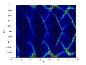
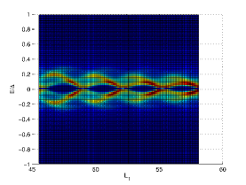
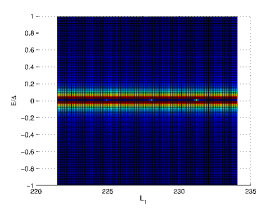
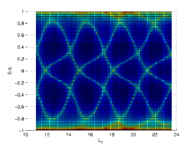
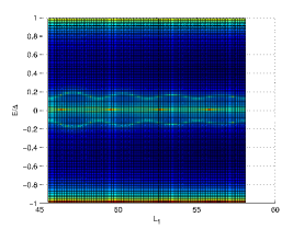
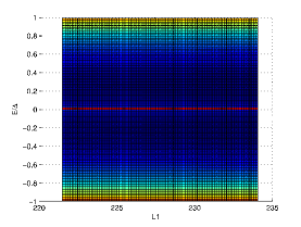
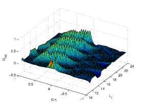
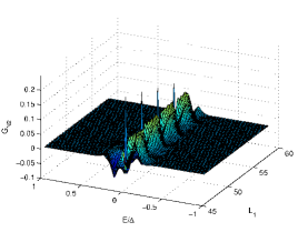
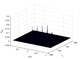
Figure 2: Plots of conductances and energies of sub-gap modes when $\Delta_{j}$ has the same sign in the three SC wires: the parameters chosen are $k_{F}=1,~{}m=0.5$ and $\Delta_{1}=\Delta_{2}=\Delta_{3}=\Delta=0.1$, so that the length scale $\eta=20$. In figures (a-c) and (g-i), the strength of the NM-SC barriers is $\lambda=5$, while in figures (d-f), we have $\lambda=\infty$ so that the NM leads do not play any role. In the first column, the length $L_{1}$ of the first SC wire varies from $3.5\pi$ to $7.5\pi$, while $L_{2}=6.7\pi$ and $L_{3}=6.3\pi$ are held fixed; $L_{j}\simeq\eta$ in all cases. In the second column, $L_{1}$ varies from $14.5\pi$ to $18.5\pi$, while $L_{2}=12.3\pi$ and $L_{3}=12.7\pi$; hence $L_{j}\simeq 2\eta$. In the third column, $L_{1}$ varies from $70.5\pi$ to $74.5\pi$, while $L_{2}=68.3\pi$ and $L_{3}=68.7\pi$; hence $L_{j}\gg\eta$. The first row shows top views of surface plots of $G_{C}$ as a function of $L_{1}$ and $E/\Delta$ lying in the gap $-\Delta<E<\Delta$. The second row shows the energies $E/\Delta$ of the sub-gap modes as a function of $L_{1}$ for a system with just three SC wires; the energies are found by the vanishing of the determinant of a matrix as explained in the text. The peaks in $G_{C}$ shown in figures (a-c) match well with the sub-gap energies shown in figures (d-f). The third row shows surface plots of $G_{N2}$ as a function of $L_{1}$ and $E/\Delta$.

In the regime of large wire lengths, the normal conductance $G_{N2}$ shows some interesting properties. From the discussion above, we would conclude that $G_{N2}$ should be very small at this length regime. But in Fig. 2 (i) we can see that $G_{N2}$ has discrete conductance peaks exactly at $E=0$ at some particular values of $L_{1}$, and $G_{N2}$ is quite high at those points. If we increase $L_{1}$ more, the value of $G_{N2}$ decreases but the peaks still remain. This shows that the peaks are robust and are solely due to the three-wire geometry of the system as these kinds of peaks do not appear in a simple NM-SC-NM system thakurathi . We find that at the locations of these conductance peaks, the amplitudes $t_{1j}$, $t_{2j}$, $t_{3j}$ and $t_{4j}$ take such values that $t_{1j}e^{-L_{j}/\xi}$, $t_{2j}e^{-L_{j}/\xi}$, $t_{3j}e^{L_{j}/\xi}$ and $t_{4j}e^{L_{j}/\xi}$ are significantly larger compared to their values when there is no conductance peak. Hence for these values of the amplitudes, the wave functions inside the SCs of the sub-gap modes are not negligible near the NM-SC junctions. So at these special points, an incoming electron from NM1 can easily enter the SC and then get transmitted to the NMs on the other sides by coupling to these sub-gap modes.

In the second column in Fig. 2, we have taken $L_{1}=14.5\pi$ to $18.5\pi$, $L_{2}=12.3\pi$ and $L_{3}=12.7\pi$. In this intermediate length regime, $L_{1}$ is of the order of the decay length $\xi$. Hence, the sub-gap modes will now hybridize with each other and their energy will split from zero. But the hybridization will be less than that in the $L_{1}<\eta$ regime. Hence the energy splitting will also be less which is evident from the top view of $G_{C}$ in Fig. 2 (b). In that plot we cannot see the six sub-gap modes separately. But there are states at non-zero energy due to the splitting, and the energy gap oscillates with $L_{1}$. The highest value of $G_{C}$ is lower than that in the $L_{1}\gg\eta$ regime as the incoming electron now has a finite probability of transmitting to the other NM leads.

The peaks in $G_{N2}$, as discussed in the large length regime, are present in this intermediate case also. But now $G_{N2}$ is non-zero at almost all values of $L_{1}$ because of the appreciable hybridization among the sub-gap modes.

Let us now compare our results with the energy plots we get for a SC box made of three SC wires. In these plots we use the same length regimes to compare it directly with our results. In Fig. 2 (d), namely, when $L_{1}<\eta$, we see that for a fixed $L_{1}$ there are four points at different energies where $D=0$. These four points correspond to the four sub-gap modes in Fig. 2 (a). We cannot see the other two modes because they are very close to $E/\Delta=\pm 1$ and are therefore beyond our resolution. This difference between the numerical results for the conductances and for the determinant occurs because in the conductance calculation the barriers at the NM-SC junctions have a finite strength while the determinant is calculated for a SC box with infinitely large barriers to the NM leads.

As we move to the intermediate length regime, Fig. 2 (e) shows that the $D=0$ lines approach zero energy; this occurs because the coupling between the sub-gap modes inside the SC box and therefore the splitting decreases. This is exactly what we see in the top view of $G_{C}$ in Fig. 2 (b).

In the large length regime all the $D=0$ lines stay almost exactly at $E=0$ for all values of $L_{1}$ as we can see from Fig. 2 (f). Now the sub-gap modes in the SC box are almost decoupled. This matches with the top view of $G_{C}$ for large length, i.e., Fig. 2 (c). We conclude that our numerical results for $G_{C}$ match well with the results we get for a SC box with infinite barriers at the three ends.

3.2  One of the $\Delta_{j}$’s with a different sign

In this section we consider the case $\Delta_{1}<0$ and $\Delta_{2},~{}\Delta_{3}>0$, but we take the magnitudes of all the $\Delta_{j}$’s to be the same. As the electron is coming from the NM1 side, the results for $\Delta_{1}<0$ are different from the cases with $\Delta_{2}<0$ or $\Delta_{3}<0$. We will again calculate the conductances for three different length regimes and the determinant for a SC box. We then analyze the numerical results to see the differences in the conductances compared to the case when all the $\Delta_{j}$’s have the same sign. We will take the same values of the parameters as before, so that the length scale $\eta=20$.

In the first column of Fig. 3, we take $L_{1}=2.5\pi$ to $6.5\pi$, $L_{2}=5.7\pi$ and $L_{3}=5.3\pi$. In this regime, from the top view of $G_{C}$ in Fig. 3 (a), we can clearly see that there are four sub-gap modes in the system. The sub-gap modes have non-zero energies as the decay length $\xi$ is greater than the length of the SCs. Instead of three sub-gap modes at the junction of three wires, there is now only one sub-gap mode. In this length regime both $G_{C}$ and $G_{N2}$ are finite as we can see from the plots. We have already discussed the reason behind this earlier when all the $\Delta_{j}$’s have the same sign.

In the third column, we choose $L_{1}=70.5\pi$ to $74.5\pi$, $L_{2}=68.3\pi$ and $L_{3}=68.7\pi$; hence $L_{1}\gg\eta$ and is therefore much larger than the decay length. Similar to the earlier case when all the $\Delta_{j}$’s are positive, here we again get $G_{C}$ almost equal to 2 (in units of $e^{2}/h$) and $G_{N2}$ close to zero as the sub-gap modes are almost decoupled. The energy splitting of the sub-gap modes is also close to zero. Instead of having different energies, now all the four sub-gap modes lie close to zero energy as we can see from Fig. 3 (c). Near the ends of the gap, i.e., $E/\Delta=\pm 1$, $G_{N2}$ rises which is due to the single particle density of states which is non-zero at those energies.

Unlike the case of all $\Delta_{j}$’s positive, $G_{N2}$ now does not show any conductance peaks at $E=0$ at any particular values of $L_{1}$. We have looked at the numerical values of $t_{1j}$, $t_{2j}$, $t_{3j}$ and $t_{4j}$ at $E=0$ and at the values of $L_{1}$ where $G_{N2}$ had peaks for the case of all $\Delta_{j}$’s positive. We find that $t_{1j}e^{-L_{j}/\xi}$, $t_{2j}e^{-L_{j}/\xi}$, $t_{3j}e^{L_{j}/\xi}$ and $t_{4j}e^{L_{j}/\xi}$ are quite large in this case also. However $t_{n3}$ and $t_{a3}$ are almost equal; hence $G_{N2}=|t_{n3}|^{2}-|t_{a3}|^{2}$ is almost equal to zero. This is an interesting difference between the cases of all $\Delta_{j}$’s having the same sign versus one of them having a different sign.

For the intermediate regime we have chosen $L_{1}=14.5\pi$ to $18.5\pi$, $L_{2}=12.7\pi$ and $L_{3}=12.7\pi$, so that $L_{1}\simeq\eta$. In Fig. 3 (b) we see the that the sub-gap modes lie very close to $E=0$. There is a small energy splitting; this splitting is due to the finite coupling of the sub-gap modes as the decay length is of the order of $L_{1}$. We find that $G_{N2}$ is almost zero and very small compared to $G_{C}$.

Next we consider a SC box and plot the determinant $D$ of the matrix of amplitudes as a function of $E/\Delta$ and $L_{1}$ as we did earlier, taking $\Delta_{1}<0$, and $\Delta_{2},~{}\Delta_{3}>0$. From the second row of Fig. 3, we can see that the $D=0$ lines match well with our numerical results for the conductance peaks in the different regimes of length.

We have checked that instead of taking $\Delta_{1}<0$, if we choose $\Delta_{2}<0$ or $\Delta_{3}<0$ all the numerical results are qualitatively similar.

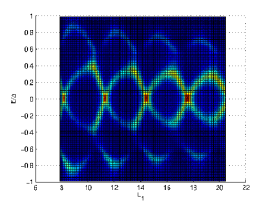
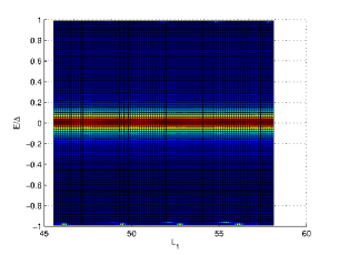
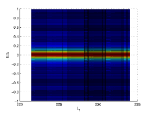
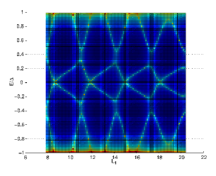
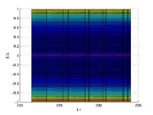
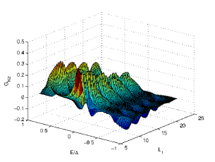
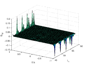
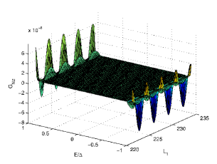
Figure 3: Plots of conductances and energies of the sub-gap modes when $\Delta_{1}<0$, while $\Delta_{2},~{}\Delta_{3}>0$: the parameters chosen are $k_{F}=1,~{}m=0.5$ and $-\Delta_{1}=\Delta_{2}=\Delta_{3}=\Delta=0.1$, so that $\eta=20$. In figures (a-c) and (g-i), the strength of the NM-SC barriers is $\lambda=5$, while in figures (d-f), we have $\lambda=\infty$ so that the NM leads do not play any role. In the first column, the length $L_{1}$ of the first SC wire varies from $3.5\pi$ to $7.5\pi$, while $L_{2}=6.7\pi$ and $L_{3}=6.3\pi$ are held fixed; $L_{j}\simeq\eta$ in all cases. In the second column, $L_{1}$ varies from $14.5\pi$ to $18.5\pi$, while $L_{2}=12.3\pi$ and $L_{3}=12.7\pi$; hence $L_{j}\simeq 2\eta$. In the third column, $L_{1}$ varies from $70.5\pi$ to $74.5\pi$, while $L_{2}=68.3\pi$ and $L_{3}=68.7\pi$; hence $L_{j}\gg\eta$. The first row shows top views of surface plots of $G_{C}$ as a function of $L_{1}$ and $E/\Delta$ lying in the gap $-\Delta<E<\Delta$. The second row shows the energies $E/\Delta$ of the sub-gap modes as a function of $L_{1}$ for a system with just three SC wires; the energies are found by the vanishing of the determinant of a matrix as explained in the text. The peaks in $G_{C}$ shown in figures (a-c) match well with the sub-gap energies shown in figures (d-f). The third row shows surface plots of $G_{N2}$ as a function of $L_{1}$ and $E/\Delta$.

We would like to point out that our results differ in many significant ways from those in earlier papers (such as Ref. thakurathi, ) which considered a single SC wire lying between two NM leads. In a single SC wire, there are only two sub-gap modes lying at the ends of the wire; they give rise to two peaks in the conductance. If the $p$-wave pairing $\Delta$ changes sign somewhere inside the wire, two more sub-gap modes appear there; however these do not have an appreciable effect on the conductances. In contrast to this, our system has several sub-gap modes, three at the NM-SC junctions and one or three at the junction of three SC wires depending on the relative signs of the $\Delta_{j}$’s. All these sub-gap modes give rise to peaks in the conductance. To the best of our knowledge, this is the first model to be studied in which there are such a large number of conductance peaks whose locations precisely match the energies of all the sub-gap modes.

4  Analytical understanding of Majorana modes at a junction of three SC wires

In this section we will study how many zero energy Majorana modes appear near a junction of three SC wires if the SC wires are semi-infinite and the NM leads are absent. Namely, the system only consists of three semi-infinite SC wires which meet at $x_{j}=0$. Therefore out of the four scattering amplitudes $t_{1j}$, $t_{2j}$,$t_{3j}$ and $t_{4j}$, only those two will be non-zero for which the SC wave function $\psi_{scj}\to 0$ as $x_{j}\to\infty$. From Eqs. (46) and (47), we know that $\psi_{scj}$ is normalizable when only $t_{1j}$ and $t_{2j}$ are non-zero. Keeping this in mind we can write down the wave functions for the semi-infinite wires.

$$\psi_{scj}~{} = ~{}t_{1j}~{}e^{ik_{1}x_{j}}~{}\left(\begin{array}[]{c}1\\ sgn(\Delta_{j})~{}e^{i\phi}\end{array}\right)$$ (57)

$$+~{}t_{2j}~{}e^{-ik_{2}x_{j}}~{}\left(\begin{array}[]{c}1\\ -sgn(\Delta_{j})~{}e^{-i\phi}\end{array}\right).$$

We want to find Majorana modes which are at zero energy and are localized near the junction. For $E=0$, $e^{i\phi}=(E-i\sqrt{\Delta^{2}-E^{2}})/\Delta$ reduces to $e^{i\phi}=-i$. Substituting this in Eq. (57), we get

$$\psi_{scj}~{} = ~{}t_{1j}e^{ik_{1}x_{j}}\left(\begin{array}[]{c}1\\ -i~{}sgn(\Delta_{j})\end{array}\right)$$ (63)

$$+t_{2j}e^{-ik_{2}x_{j}}\left(\begin{array}[]{c}1\\ -i~{}sgn(\Delta_{j})\end{array}\right).$$

Now we use the boundary conditions in Eqs. (13) to find the Majorana modes. Using (13), for the $c_{j}$’s we get

$$ik_{1}~{}t_{1j}~{}-~{}ik_{2}~{}t_{2j}$$

$$=~{}M_{j1}~{}(t_{11}+t_{21})~{}+~{}M_{j2}~{}(t_{12}+t_{22})$$

$$~{}~{}+~{}M_{j3}~{}(t_{13}+t_{23})$$

$$~{}~{}-~{}\frac{m|\Delta_{j}|}{k_{F}}(t_{1j}+t_{2j}),$$ (64)

while for the $d_{j}$’s we get,

$$sgn(\Delta_{j})~{}[ik_{1}~{}t_{1j}-ik_{2}~{}t_{2j}]$$

$$=~{}M_{j1}~{}sgn(\Delta_{1})~{}(t_{11}+t_{21})$$

$$~{}~{}+~{}M_{j2}~{}sgn(\Delta_{2})~{}(t_{12}+t_{22})$$

$$~{}~{}+~{}M_{j3}~{}sgn(\Delta_{3})~{}(t_{13}+t_{23})$$

$$~{}~{}-~{}\frac{m|\Delta_{j}|~{}sgn(\Delta_{j})}{k_{F}}~{}(t_{1j}+t_{2j}).$$ (65)

So we have a total of six equations, three for the $c_{j}$’s and three for the $d_{j}$’s. From Eqs. (64) and (65) it can be shown that if all the $\Delta_{j}$’s have the same sign, the equations for the $c$’s and $d$’s are exactly the same. So instead of six equations we get only three independent equations. But we have six variables in this problem since we have three wires and each of the wires has two different scattering amplitudes corresponding to $k_{1}$ and $k_{2}$. Hence we have three equations for six variables. Hence, there are three independent solutions and therefore three Majorana modes at the junction.

Now we consider the case when one of the $\Delta_{j}$’s has a different sign from the other two; let us assume that $\Delta_{2}$ and $\Delta_{3}$ have the same sign while $\Delta_{1}$ has the opposite sign. In this case, it is straightforward to show that $t_{11}+t_{21}=0$. So we now have five independent variables instead of six. Using the above relation it can be shown that the equations for $c_{2}$ and $c_{3}$ are the same as the equations for $d_{2}$ and $d_{3}$ respectively. But the equations for $c_{1}$ and $d_{1}$ are different. So we have four independent equations and five variables which implies that we have only one independent solution and hence only one Majorana mode.

These are the only two combinations of the signs of $\Delta_{j}$’s which will give different results. Eq. (14) implies that any other combination will be similar to either the first case or the second case. To summarize, the two cases are as follows.

(i) If all three $\Delta_{j}$’s have the same sign then there are three Majorana modes at the junction.

(ii) If one of the $\Delta_{j}$’s has the opposite sign to the other two then there is only one Majorana mode at the junction.

The existence of one or three zero energy Majorana modes can also be understood as follows. A well known lattice model of a $p$-wave superconducting wire is the Kitaev chain kitaev1 . We first consider a single Kitaev chain. The electron operators $c_{n}$ and $c_{n}^{\dagger}$ at site $n$ can be written in terms of two Hermitian operators, called $a_{n}$ and $b_{n}$, as $c_{n}=(1/2)(a_{n}+ib_{n})$ and $c_{n}^{\dagger}=(1/2)(a_{n}-ib_{n})$. (These operators satisfy the anticommutation relations $\{a_{m},a_{n}\}=\{b_{m},b_{n}\}=2\delta_{mn}$). The Hamiltonian of the Kitaev chain only has terms of the form $ia_{m}b_{n}$, not $ia_{m}a_{n}$ or $ib_{m}b_{n}$. Such a Hamiltonian has an “effective time reversal symmetry”, namely, it is invariant under complex conjugation of all complex numbers along with $a_{n}\to a_{n}$ and $b_{n}\to-b_{n}$ degottardi2 . This symmetry implies that if we look at eigenstates with zero energy, their wave functions involve only the $a_{n}$ or only the $b_{n}$, not both. A long Kitaev chain has zero energy Majorana modes at the two ends. Depending on the sign of the $p$-wave pairing, positive or negative, it turns out that the Majorana mode at the left end is of type $a$ and at the right end is of type $b$ or vice versa degottardi2 . We now consider three semi-infinite Kitaev chains which meet at one site; the three Kitaev chains could have the same or different signs of the $\Delta_{j}$’s. If all the $\Delta_{j}$’s have the same sign, the three Majorana modes at the junction will all be of the same type, say, $a$. Then they will not mix with each other since the Hamiltonian has no terms of the form $ia_{m}a_{n}$; hence they will remain at zero energy. On the other hand, if one of $\Delta_{j}$’s has a different sign from the other two, two of the Majorana modes will be of one type, say $a$, and the other will be of type $b$. Now the $b$ mode can mix with the two $a$’s; as a result the energies of two of the Majorana modes will become non-zero, namely $\pm E$, while one Majorana mode will stay at zero energy. (Written in terms of the $a$ and $b$ operators, the Hamiltonian of the system can be seen to have an $E\to-E$ symmetry; hence states can mix and move away from zero energy only in pairs).

Having seen that a Kitaev chain has two kinds of Majorana end modes, called $a$ and $b$, we can write down an effective Hamiltonian which describes the sub-gap physics of our three-wire system. This Hamiltonian will only contain the operators for the Majorana end modes (the operators in the rest of the SC wires are not required) and the electron operators in the NM wires fu ; fidkowski2 ; hutzen ; affleck . The Hamiltonian will have three kinds of terms. First, the Hamiltonian at the junction of the three SC wires can be written as follows. If all three Majorana modes are of the same type, then no coupling between them is allowed due to the effective time reversal symmetry. But if two of the modes are of one type (say, type $a$ on wires 1 and 2) and the third mode is of the other type ($b$ on wire 3), then this part of the Hamiltonian will take the form $H_{1}=i(w_{1}a_{1}+w_{2}a_{2})b_{3}$, where $w_{1}$ and $w_{2}$ are two couplings (assumed to be real). Next, on each wire $j$, the Majorana mode near the junction with the NM wire is of the opposite type to the mode near the junction of the three SC wires; namely, at the junctions with NM wires, the modes will be given by $b_{1}$, $b_{2}$ and $a_{3}$. The hybridization between the two modes at the ends of each wire will give rise to three more couplings given by $H_{2}=i(w_{3}a_{1}b_{1}+w_{4}a_{2}b_{2}+w_{5}a_{3}b_{3})$. (The couplings $w_{3}$, $w_{4}$ and $w_{5}$ go to zero exponentially as the lengths of the SC wires become large). Finally, we have couplings at the junctions of the SC and NM wires between the Majorana modes at $x_{j}=L_{j}-\epsilon$ and the electron operators in the NM wires at $x_{j}=L_{j}+\epsilon$ (following the notation in Eq. (1)). We can think of this coupling as arising from a hopping between the operator $c_{sc}=(1/2)(a+ib)$ at $x_{j}=L_{j}-\epsilon$ in the SC wire and the operator $c_{nm}$ at $x_{j}=L_{j}+\epsilon$ in the NM wire, namely, a term of the form $c_{sc}^{\dagger}c_{nm}+c_{nm}^{\dagger}c_{sc}$. If the Majorana mode is of type $a$, we set $b=0$ and get $c_{sc}^{\dagger}c_{nm}+c_{nm}^{\dagger}c_{sc}=(1/2)a(c_{nm}-c_{nm}^{\dagger})$, while if the Majorana is of type $b$, we set $a=0$ and get $c_{sc}^{\dagger}c_{nm}+c_{nm}^{\dagger}c_{sc}=-(i/2)b(c_{nm}+c_{nm}^{\dagger})$. We thus get a coupling of the form

$$H_{3} = iw_{6}~{}b_{1}~{}[c_{nm}(L_{1}+\epsilon)+c_{nm}^{\dagger}(L_{1}+\epsilon)]$$ (66)

$$+~{}iw_{7}~{}b_{2}[c_{nm}(L_{2}+\epsilon)+c_{nm}^{\dagger}(L_{2}+\epsilon)]$$

$$+~{}w_{8}~{}a_{3}[c_{nm}(L_{3}+\epsilon)-c_{nm}^{\dagger}(L_{3}+\epsilon)].$$

The complete effective Hamiltonian is given by the sum of $H_{1}$, $H_{2}$ and $H_{3}$ and has eight parameters $w_{i}$.

The parameters $w_{i}$ can be determined as follows. We first use the microscopic Hamiltonian in Eq. (1), the $\delta$-function potentials $\lambda$ at the NM-SC junctions and the matrix $\bf M$ at the junction of three SCs to compute the energies and wave functions of all the sub-gap modes. We then fit the values of these quantities with those calculated from the effective Hamiltonian described above in order to find the values of $w_{i}$. We will not carry out this exercise here. The effective Hamiltonian can then be used to compute the various conductances of the system fidkowski2 .

5  Renormalization group equations for a junction of several wires

In this section, we will consider the effect of electron-electron interactions on the conductances of a system of two or more NM wires which meet at a junction where there is a SC region (we can consider this region to be a SC dot). This system differs from the one studied in the earlier sections in two major ways. First, the region of three SC wires considered in Sects. 2 - 4 will now be taken to be a single region. Further, the only role played by this region will be to give rise to a scattering matrix $S$ for the NM wires. Due to the superconductivity, we have to consider the cases of both incident electrons and incident holes, and both normal and Andreev reflection and transmission processes; $S$ will therefore be a $2N\times 2N$ matrix for the case of $N$ NM wires meeting at the junction with the SC region. Second, we will only study the conductances at energies much larger than $\Delta$, in contrast to the earlier sections where we only looked at the sub-gap conductances. The reason for considering energies much larger than $\Delta$ (but much smaller than the band width of the system) is that the analysis given below only works when the conductances are slowly varying functions of the energy; this will become clearer as we proceed. We will take the interactions to be present only in the NM wires and derive RG equations which will tell us how the $S$-matrix evolves when we start at the length scale of the SC region and then increase the length scale to expand from that region into the NM wires.

In one dimension, the technique of bosonization is often used to study systems with short-range density-density interactions gogolin ; in this method a system of interacting fermions is mapped to a system of non-interacting bosons. This method has the advantage that interactions of any strength can be dealt with. However this method runs into difficulties in the presence of junctions of three or more wires and superconductivity for the following reasons. As we have seen, a junction is characterized by a matrix $\bf M$ which relates the electron fields on different wires in a linear way. Since bosonization relates electron operators to exponentials of bosonic operators, a linear relation between fermionic fields in different wires translates, in general, to a non-linear relation between the bosonic fields; this makes it difficult to use bosonization. (However, there are some special forms of the junction matrix when bosonization can be applied. These special cases correspond to the magnitudes of all the reflection or transmission amplitudes being equal to either zero or 1, namely, either perfect reflection and no transmission, or no reflection and perfect transmission lal ). Next, bosonization works best if the system is gapless and the energy-momentum dispersion is linear for both the fermionic and the bosonic theories which are related to each other. However superconductivity produces a gap proportional to the SC pairing $\Delta$, and the dispersion is not linear for energies of the same order as $\Delta$. So bosonization works only if we treat $\Delta$ as a perturbation (as was done in Ref. ganga, for example).

We will therefore use a different approach which directly uses the fermionic language yue ; lal ; das2 ; saha . Unlike bosonization, this approach is useful only if the interaction strengths are weak in all the wires. However it has the advantage that it works for any form of the scattering matrix which characterizes the junction. The results obtained by this method and those obtained by bosonization will of course match in the parameter regimes where both methods work, namely, when the interactions are weak and the junction scattering matrix has some special forms. We will now describe this method in detail.

We begin with a second quantized fermionic field $c(x)$ and the corresponding hole field $d(x)$, where $d(x)=c^{\dagger}(x)$, for a single semi-infinite NM wire which goes from $x=0$ to $\infty$ and is connected to a SC region at $x=0$. At low temperatures, only low-energy processes are of interest and these only involve modes near the Fermi momenta $\pm k_{F}$; we will therefore consider only these modes. We therefore write the second-quantized field $c(x)$ as

$$c(x)~{}=~{}c_{I}(x)e^{-ik_{F}x}~{}+~{}c_{O}(x)e^{ik_{F}x},$$ (67)

where $c_{I}$ and $c_{O}$ denote the fields of incoming and outgoing electrons respectively. We take these fields to be slowly varying on the length scale of $1/k_{F}$ as we have separated out the rapidly varying factors $e^{\pm ik_{F}x}$. Namely, the fields $c_{I},~{}c_{O}$ have momentum components $k$ such that $|k|\ll k_{F}$. We can then use a linear approximation for the dispersion relations of these fields so that $E=\pm v_{F}k$ for $c_{I}$ and $c_{O}$ respectively, with $v_{F}$ being the Fermi velocity.

Similarly, for the second-quantized field $d(x)$ we write

$$d(x)~{}=~{}d_{I}(x)e^{ik_{F}x}~{}+~{}d_{O}(x)e^{-ik_{F}x}.$$ (68)

Note that the rapidly varying exponential terms multiplying $d_{I}$ and $d_{O}$ are the opposite of those multiplying $c_{I}$ and $c_{O}$. This is because destroying an electron is equivalent to creating a hole, so that $E_{h}=-E_{e}$ where $E_{h}$ and $E_{e}$ are the energies of the electron and hole respectively.

Let us now introduce a short-ranged density-density interaction between the electrons of the form

$$H_{int}~{}=~{}\frac{1}{2}~{}\int\int dxdy~{}\rho(x)V(x-y)\rho(y).$$ (69)

We assume that $V(x)$ is a real and even function of $x$. The density $\rho$ is a function of the second quantized fields given by $\rho(x)=c^{\dagger}(x)c(x)=d(x)d^{\dagger}(x)=-d^{\dagger}(x)d(x)$ (using the anticommutation property of the fermionic fields). Using Eq. (67), we obtain the expectation values

$$<\rho(x)> = <c^{\dagger}_{I}c_{I}>~{}+~{}<c^{\dagger}_{O}c_{O}>$$

$$+~{}<c^{\dagger}_{I}c_{O}>e^{2ik_{F}x}~{}+~{}<c^{\dagger}_{O}c_{I}>e^{-2ik_{F}x}.$$

Next, we will assume that $V(x)$ is so short-ranged that $x$ and $y$, which appear as arguments of the density fields, can be set equal to each other except when the corresponding term in $H_{int}$ becomes zero. Using this assumption and the anticommutation relation between the fermionic fields, we get

$$H_{int}~{}=~{}g~{}\int dx~{}c^{\dagger}_{I}c_{I}c^{\dagger}_{O}c_{O},$$ (71)

where $g$ is related to the Fourier transform of $V(x)$ as $g=\tilde{V}(0)-\tilde{V}(2k_{F})$. From this expression it is clear that $g=0$ if $V(x)$ is a $\delta$-function. Hence $V(x)$ must have a finite range for the interaction to have an effect. For each NM wire, the interaction is described by the single parameter $g$. The value of this parameter may be different for different wires which we will denote by $g_{j}$ on wire $j$. We define a dimensionless quantity $\alpha_{j}$ as

$$\alpha_{j}=\frac{g_{j}}{2\pi v_{F}},$$ (72)

where we assume $v_{F}$ to be the same in all the NM wires.

Let us briefly discuss how the interaction parameter appears in the formalism of bosonization. For spinless fermions, which is relevant here as we are studying $p$-wave SCs, the bosonic theory is characterized by two quantities, the velocity $v$ of the excitations and a dimensionless parameter $K$ (called the Luttinger parameter) which is a measure of the strength of the interactions between the fermions. These are related to $v_{F}$ and $\alpha$ as

$$v = v_{F}(1-\alpha^{2})^{1/2},$$

$$K = \left(\frac{1-\alpha}{1+\alpha}\right)^{1/2}.$$ (73)

Note that $K=1$ if $\alpha=0$ (non-interacting fermions), while $K<1$ ($K>1$) for $\alpha>0$ ($\alpha<0$), namely, repulsive (attractive) interactions. For weak interactions we get $v=v_{F}$ and $K=1-\alpha$ to first order in $\alpha$. We will do our RG analysis in the limit that $\alpha$ is small and positive in each wire.

As we have discussed earlier, it is generally difficult to bosonize a system with junctions. We will therefore use a different method which will enable us to derive RG equations directly for the scattering matrix of the junction. As we will see, this method only works up to first order in the interaction parameters $\alpha_{j}$. The basic idea of this method is the following. In the presence of non-zero reflection amplitudes $r_{jj}$ at the junction, the density of non-interacting fermions in the NM wire $j$ will have Friedel oscillations with wave number $2k_{F}$. When an interaction is turned on, an electron can scatter to an electron or a hole (Andreev reflection) from these oscillations with an amplitude which is proportional to the parameter $\alpha_{j}$. Ref. yue, used this idea to derive RG equations for an arbitrary $S$-matrix describing the junction of two semi-infinite wires. An RG analysis was then done for junctions of more than two wires, without superconductivity in Refs. lal, and das2, and with a $s$-wave superconducting junction in Ref. saha, . We will carry out an RG analysis for our system where several NM wires meet at a junction with a $p$-wave SC region. We expect the results to be much richer than those for a junction of NM wires when no superconductivity is present.

We will begin our analysis by deriving the form of the density oscillations in one particular NM wire close to the junction with the SC region. We will consider separately the cases of an electron and a hole coming in from a NM lead.

5.1  Processes related to an incoming electron

An incoming electron can be either

(i) normally reflected with amplitude $r_{ee}$, or

(ii) Andreev reflected to a hole with amplitude $r_{he}$.

For momenta near $k_{F}$ we can write the wave functions for electrons and holes as

$$c_{k}(x) = c_{I}e^{-ik_{F}x}~{}+~{}c_{O}e^{ik_{F}x}$$

$$= e^{-i(k_{F}+k)x}~{}+~{}r_{ee}e^{i(k_{F}+k)x},$$

$$d_{k}(x) = d_{O}e^{-ik_{F}x}~{}=~{}r_{he}e^{-i(k_{F}-k)x},$$ (74)

where $|k|\ll k_{F}$. In the ground state of a non-interacting system, all the energy states below the Fermi energy $E_{F}$ are filled for electrons; this corresponds to negative values of $k$ in Eq. (74). Although we are only interested in values of $k$ close to zero, it is mathematically convenient to take the range of $k$ to be $-\infty$ to $\infty$ even though the range is finite and given by the band width in real systems. The expectation value of $\rho(x)$ in terms of $c_{k}(x)$ is given by

$$<\rho(x)>~{}=~{}\int_{-\infty}^{0}\frac{dk}{2\pi}~{}c^{*}_{k}c_{k},$$ (75)

where we have taken the lower limit of $k$ to be $-\infty$. We see that $<\rho>$ has a constant piece $\rho_{0}$ which can be eliminated by normal ordering. We are then left with

$$<\rho(x)>~{}-~{}\rho_{0}~{}=~{}\frac{i}{4\pi x}(r^{*}_{ee}e^{-2ik_{F}x}~{}-~{}r_{ee}e^{2ik_{F}x}).$$ (76)

It is clear that these terms arise entirely due to the interference between the incoming and reflected waves. Substituting Eq. (76) in Eq. (LABEL:int2) we see that $<c^{\dagger}_{I}c_{I}+c^{\dagger}_{O}c_{O}>=\rho_{0}$ is a constant, while

$$<c^{\dagger}_{O}c_{I}> = \frac{ir^{*}_{ee}}{4\pi x},$$

$$<c^{\dagger}_{I}c_{O}> = <c^{\dagger}_{O}c_{I}>^{*}~{}=~{}-~{}\frac{ir_{ee}}{4\pi x}.$$ (77)

An important point to note here is that there will also be a contribution to $c(x)$ and therefore to $<\rho(x)>$ from the waves which are transmitted from the other wires. As a wave transmitted to one wire from any other wire is incoherent with the incident and reflected waves of the first wire (we are assuming that waves incident from different NM leads are phase incoherent with respect to each other), there is no interference between these waves. Since the waves transmitted from the other wires only contribute to an outgoing wave in this wire, there is no interference and their contribution to $<\rho(x)>$ is independent of $x$. Hence, it can be absorbed in $\rho_{0}$. We conclude that the Friedel oscillations in Eq. (76) in a given wire arises only from the reflections within that wire.

Now, in our system we have both normal and Andreev reflections. So there will be some non-zero expectation values for the operators which connect electrons and holes such as $c^{\dagger}_{I}d_{O}$ and $d^{\dagger}_{O}c_{I}$. Using Eq. (74), we find that the expectation values of these operators are given by

$$<c^{\dagger}_{I}d_{O}> = \int_{-\infty}^{0}\frac{dk}{2\pi}~{}r_{he}e^{i2kx}~{}=~{}-~{}\frac{ir_{he}}{4\pi x},$$

$$<d^{\dagger}_{O}c_{I}>~{} = ~{}\frac{ir^{*}_{he}}{4\pi x}.$$ (78)

To evaluate the integral in the first equation in (78), we must introduce a factor like $e^{\epsilon k}$ which cuts off the contribution from the lower limit $k\to-\infty$, and we then take the limit $\epsilon\to 0$. Further, we have assumed that $r_{he}$ varies slowly with $k$ so that it is a reasonable approximation to take it outside the integral over $k$ in the first equation. This is the reason why our analysis only works at energies which lie far from the SC gap; for those energies the reflection and transmission amplitudes are slowly varying functions of the energy. In contrast to this, the sub-gap conductances have sharp peaks due to various sub-gap modes; hence the reflection and transmission amplitudes are not slowly varying functions of the energy if it lies inside the SC gap. We note that a renormalization group study at energies within or close to the SC gap, where the reflection and transmission amplitudes vary rapidly, has been carried out in Ref. titov, .

Next, we derive the reflections of the electrons and holes from the Friedel oscillation by using the Hartree-Fock decomposition of the Hamiltonian in Eq. (71). We have

$$H_{int} = -g~{}\int_{0}^{\infty}dx~{}[<c^{\dagger}_{I}c_{O}>c^{\dagger}_{O}c_{I}~{}+<c^{\dagger}_{O}c_{I}>c^{\dagger}_{I}c_{O}$$ (79)

$$~{}~{}~{}~{}~{}~{}+<c^{\dagger}_{I}c^{\dagger}_{O}>c_{I}c_{O}~{}+<c_{I}c_{O}>c^{\dagger}_{I}c^{\dagger}_{O}].$$

Using the expectation values of the various operators derived earlier and the identities $c_{I}c_{O}=c_{I}d_{O}^{\dagger}=-d_{O}^{\dagger}c_{I}$ and $c_{I}^{\dagger}c_{O}^{\dagger}=c_{I}^{\dagger}d_{O}$, we obtain

$$H_{int} = \frac{g}{4\pi}~{}\int_{0}^{\infty}\frac{dx}{x}~{}[ir_{ee}c^{\dagger}_{O}c_{I}~{}-~{}ir^{*}_{ee}c^{\dagger}_{I}c_{O}$$ (80)

$$~{}~{}~{}~{}~{}~{}~{}~{}~{}~{}-~{}ir_{he}d^{\dagger}_{O}c_{I}~{}+~{}ir^{*}_{he}c^{\dagger}_{I}d_{O}].$$

We can now derive the amplitude to go from an incoming wave to an outgoing wave under the action of $\exp(-iH_{int}t)$. We begin with an incoming electron with momentum $k$. Various processes can now occur.

(i) An incoming electron with momentum $k$ can go to an outgoing electron with momentum $k^{\prime}$ under the action of $H_{int}$. The corresponding amplitude is

$$-i~{}\int\frac{dk^{\prime}}{2\pi}~{}2\pi\delta(E_{k}-E_{k^{\prime}})$$

$$\times~{}<outgoing,e,k^{\prime}|H_{int}|incoming,e,k>$$

$$=~{}\frac{g}{4\pi v_{F}}~{}\int_{0}^{\infty}\frac{dx}{x}~{}r_{ee}~{}e^{-2ikx}.$$ (81)

To obtain the above expression we have used Eq. (79), the dispersion relation $E=v_{F}k$ (which implies $\delta(E_{k}-E_{k^{\prime}})=(1/v_{F})\delta(k-k^{\prime})$), and the wave functions $e^{\pm{i(k_{F}+k)x}}$ of the outgoing and incoming electrons respectively.

To derive RG equations for quantities like $r_{ee}$ from Eq. (81), we will integrate $x$ over a small interval going from $L$ to $L+dL=Le^{dl}$. Here $l$ is the logarithm of the length scale, and we can write $l=ln(L/a)$, where $a$ is a short distance scale (which is the size of the superconducting region forming the junction) from which we will begin to integrate the RG equations. Eq. (81) then gives

$$\frac{gr_{ee}}{4\pi v_{F}}~{}dl~{}=~{}\frac{\alpha r_{ee}}{2}~{}dl,$$ (82)

where we have used Eq. (72).

(ii) Similarly we find that the amplitude to go from an outgoing electron to an incoming electron is given by

$$-~{}\frac{\alpha r^{*}_{ee}}{2}~{}dl.$$ (83)

(iii) Due to the presence of the SC region, Andreev reflection can also occur, namely, an incoming electron can go to an outgoing hole under the action of $H_{int}$ as given in Eq. (79). We can calculate the amplitude of this process in the same way as we did for normal reflection above. The amplitude to go from an incoming electron with momentum $k$ to an outgoing hole with momentum $k^{\prime}$ is found to be

$$-~{}\frac{\alpha r_{he}}{2}~{}dl.$$ (84)

(iv) The amplitude to go from an outgoing hole to an incoming electron is given by

$$\frac{\alpha r^{*}_{he}}{2}~{}dl.$$ (85)

This completes the list of processes which can occur if we start with an incoming electron.

5.2  Processes related to an incoming hole

All the processes we discussed in the previous section can be studied if we start with an incoming hole. An incoming hole can be either

(i) normally reflected to another hole with amplitude $r_{hh}$, or

(ii) Andreev reflected to an electron with amplitude $r_{eh}$.

For momenta near $k_{F}$ we can write the hole and electron wave functions as

$$d_{k}(x) = d_{I}e^{ik_{F}x}~{}+~{}d_{O}e^{-ik_{F}x}$$

$$= e^{i(k_{F}-k)x}~{}+~{}r_{hh}e^{-i(k_{F}-k)x},$$

$$c_{k}(x) = c_{O}e^{ik_{F}x}~{}=~{}r_{eh}e^{i(k_{F}+k)x}.$$ (86)

For holes, we can use Eq. (75) and the fact that $c^{\dagger}c=dd^{\dagger}=-d^{\dagger}d$ (plus a constant) to write the ground state expectation value of $\rho(x)$ as

$$<\rho(x)>~{}=~{}-~{}\int_{-\infty}^{0}\frac{dk}{2\pi}~{}d^{*}_{k}d_{k}.$$ (87)

We can then find expectation values of various operators following a procedure similar to the previous section. We obtain

$$<d^{\dagger}_{I}d_{O}> = -\frac{ir_{hh}}{4\pi x},$$

$$<d^{\dagger}_{O}d_{I}> = \frac{ir^{*}_{hh}}{4\pi x},$$

$$<c^{\dagger}_{O}d_{I}> = \frac{ir^{*}_{eh}}{4\pi x},$$

$$<d^{\dagger}_{I}c_{O}> = -\frac{ir_{eh}}{4\pi x}.$$ (88)

Using these expectation values we find the amplitudes of various processes.

(i) Under the action of $H_{int}$, an incoming hole goes to an outgoing hole with an amplitude

$$\frac{\alpha r_{hh}}{2}~{}dl.$$ (89)

(ii) An outgoing hole goes to an incoming hole with an amplitude

$$-~{}\frac{\alpha r^{*}_{hh}}{2}~{}dl.$$ (90)

(iii) An incoming hole goes to an outgoing electron with an amplitude

$$-~{}\frac{\alpha r_{eh}}{2}dl.$$ (91)

(iv) An outgoing electron goes to an incoming hole with an amplitude

$$\frac{\alpha r^{*}_{eh}}{2}dl.$$ (92)

5.3  RG equations for the reflection and transmission amplitudes

The amplitudes of all the processes that we derived earlier can now be combined along with the $S$-matrix at a junction of several NM wires with a SC region to calculate corrections to the $S$-matrix. We will calculate all the corrections to first order in the interaction parameters $\alpha_{j}$.

We first consider corrections to the reflection amplitude $r_{ee,jj}$ on wire $j$. To first order in $\alpha_{j}$, this gets contributions from the following processes. An incoming electron on wire $j$ can

(i) become an outgoing electron on the same wire by scattering from the Friedel oscillations in the density with the amplitude given in Eq. (82).

(ii) reflect from the junction with amplitude $r_{ee,jj}$ to become an outgoing electron, then become an incoming electron due to the Friedel oscillations according to (83), and finally reflect from the junction as an electron with amplitude $r_{ee,jj}$.

(iii) reflect from the junction with amplitude $r_{ee,jj}$ to become an outgoing electron, become an incoming hole due to Friedel oscillations according to (92), and then Andreev reflect from the junction as an electron with amplitude $r_{eh,jj}$.

(iv) Andreev reflect from the junction with amplitude $r_{he,jj}$ to become an outgoing hole, become an incoming electron due to Friedel oscillations according to (85), and then reflect from the junction as an electron with amplitude $r_{ee,jj}$.

(v) become an outgoing hole by Andreev reflection from the junction with amplitude $r_{he,jj}$, become an incoming hole due to Friedel oscillations according to (90), and then Andreev reflect from the junction as an electron with amplitude $r_{eh,jj}$.

(vi) transmit through the junction to wire $i$ (with $i\neq j$) as an electron with amplitude $t_{ee,ij}$, turn from an outgoing electron to an incoming electron on wire $i$ due to Friedel oscillations according to (83), and then transmit through the junction to wire $j$ as an electron with amplitude $t_{ee,ji}$.

(vii) transmit through the junction into wire $i$ as an electron with amplitude $t_{ee,ij}$, turn from an outgoing electron to an incoming hole on wire $i$ according to (92), and then transmit to wire $j$ as an electron with amplitude $t_{eh,ji}$.

(viii) transmit through the junction into wire $i$ as a hole with amplitude $t_{he,ij}$, turn from an outgoing hole to an incoming electron on wire $j$ according to (85), and then transmit to wire $i$ as an electron with amplitude $t_{ee,ji}$.

(ix) transmit through the junction into wire $i$ as a hole with amplitude $t_{he,ij}$, turn from an outgoing hole to an incoming hole on wire $j$ according to (90), and then transmit to wire $j$ as an electron with amplitude $t_{eh,ji}$.

Collecting all these terms, we find that the correction to $r_{ee,jj}$ is given by

$$dr_{ee,jj} = B_{ee,jj}~{}dl,$$

$$B_{ee,jj} = \frac{1}{2}[\alpha_{j}r_{ee,jj}-\alpha_{j}|r_{ee,jj}|^{2}r_{ee,jj}+\alpha_{j}|r_{eh,jj}|^{2}r_{ee,jj}$$

$$+\alpha_{j}|r_{he,jj}|^{2}r_{ee,jj}-\alpha_{j}r_{he,jj}r_{hh,jj}^{*}r_{eh,jj}$$

$$+\sum_{i\neq j}(-\alpha_{i}t_{ee,ji}r_{ee,ii}^{*}t_{ee,ij}+\alpha_{i}t_{ee,ji}r_{eh,ii}^{*}t_{eh,ij}$$

$$~{}~{}~{}~{}+\alpha_{i}t_{he,ji}r_{he,ii}^{*}t_{ee,ij}-\alpha_{i}t_{he,ji}r_{hh,ii}^{*}t_{eh,ij})].$$

Similarly, the transmission amplitude $t_{ee,ji}$ from wire $i$ to wire $j$ can get corrections from the following processes. The incoming electron on wire $i$ can

(i) get reflected from the junction as an electron with amplitude $r_{ee,ii}$, then become an incoming electron according to (83), and finally transmit to wire $j$ as an electron with amplitude $t_{ee,ji}$.

(ii) reflect from the junction as an electron with amplitude $r_{ee,ii}$, become an incoming hole according to (92), and then transmit to wire $j$ as an electron with amplitude $t_{eh,ji}$.

(iii) Andreev reflect from the junction as a hole with amplitude $r_{he,ii}$, become an incoming electron according to (85), and then transmit to wire $j$ as an electron with amplitude $t_{ee,ji}$.

(iv) Andreev reflect from the junction as a hole with amplitude $r_{he,ii}$, become an incoming hole according to (90), and then transmit to wire $j$ as an electron with amplitude $t_{eh,ji}$.

(v) transmit to wire $j$ as an electron with amplitude $t_{ee,ji}$, become an incoming electron on wire $j$ according to (83), and then reflect from the junction as an electron with amplitude $r_{ee,jj}$.

(vi) transmit to wire $j$ as an electron with amplitude $t_{ee,ji}$, become an incoming hole on wire $j$ according to (92), and then reflect from the junction as an electron with amplitude $r_{eh,jj}$.

(vii) transmit to wire $j$ as a hole with amplitude $t_{he,ji}$, become an incoming electron on wire $j$ according to (85), and then reflect from the junction as an electron with amplitude $r_{ee,jj}$.

(viii) transmit to wire $j$ as a hole with amplitude $t_{he,ji}$, become an incoming hole on wire $j$ according to (90), and then reflect from the junction as an electron with amplitude $r_{eh,jj}$.

(ix) transmit to wire $k$ (with $k\neq i,~{}j$) as an electron with amplitude $t_{ee,ki}$, become an incoming electron according to (83), and then transmit to wire $j$ as an electron with amplitude $t_{ee,jk}$.

(x) transmit to wire $k$ as an electron with amplitude $t_{ee,ki}$, become an incoming hole according to (92), and then transmit to wire $j$ with amplitude $t_{eh,jk}$.

(xi) transmit to wire $k$ as a hole with amplitude $t_{he,ki}$, become an incoming electron according to (85), and then transmit to wire $j$ with amplitude $t_{ee,jk}$.

(xii) transmit to wire $k$ as a hole with amplitude $t_{he,ki}$, become an incoming hole according to (90), and then transmit to wire $j$ with amplitude $t_{eh,jk}$.

Hence the total correction to $t_{ee,ji}$ is given by

$$dt_{ee,ji} = B_{ee,ji}~{}dl,$$

$$B_{ee,ji} = \frac{1}{2}[-\alpha_{i}t_{ee,ji}|r_{ee,ii}|^{2}+\alpha_{i}t_{eh,ji}r_{ee,ii}r_{eh,ii}^{*}$$ (94)

$$+\alpha_{i}t_{ee,ji}|r_{he,ii}|^{2}-\alpha_{i}t_{eh,ji}r_{he,ii}r_{hh,ii}^{*}$$

$$-\alpha_{j}|r_{ee,jj}|^{2}t_{ee,ji}+\alpha_{j}|r_{eh,jj}|^{2}t_{ee,ji}$$

$$+\alpha_{j}r_{ee,jj}r_{he,jj}^{*}t_{he,ji}-\alpha_{j}r_{eh,jj}r_{hh,jj}^{*}t_{he,ji}$$

$$+\sum_{k\neq i,j}(-\alpha_{k}t_{ee,jk}r_{ee,kk}^{*}t_{ee,ki}$$

$$+\alpha_{k}t_{eh,jk}r_{eh,kk}^{*}t_{ee,ki}+\alpha_{k}t_{ee,jk}r_{he,kk}^{*}t_{he,ki}$$

$$-\alpha_{k}t_{eh,jk}r_{hh,kk}^{*}t_{he,ki})].$$

Similarly, we can find the corrections to all the other entries of the $S$-matrix, namely, $r_{hh,jj},~{}r_{he,jj},~{}r_{eh,jj},~{}t_{hh,ji},~{}t_{he,ji}$ and $t_{eh,ji}$. We now consider all these components of $S$ to be functions of a length scale $L$, where $L$ can vary all the way from a short distance scale $a$ to a large distance scale which may be either the length of the NM wires or the thermal coherence length as discussed in Sect. 6.2. $L$ and $l$ are related as $l=ln(L/a)$, so that $l=0$ when $L=a$. Eqs.(LABEL:r1-94) then give us the RG equations

$$\frac{dr_{ee,jj}}{dl} = B_{ee,jj},$$

$$\frac{dt_{ee,ji}}{dl} = B_{ee,ji}.$$ (95)

Eqs. (95) can be written in a more compact way. Given the matrix $S$ and the parameters $\alpha_{j}$, we define a matrix $F$ whose non-zero elements are

$$F_{ee,jj} = \frac{1}{2}\alpha_{j}r_{ee,jj},$$

$$F_{eh,jj} = -~{}\frac{1}{2}\alpha_{j}r_{eh,jj},$$

$$F_{he,jj} = -~{}\frac{1}{2}\alpha_{j}r_{he,jj},$$

$$F_{hh,jj} = \frac{1}{2}\alpha_{j}r_{hh,jj}.$$ (96)

We can then show that the RG equations for the different elements of $S$ (such as $r_{ee,jj}$ and $t_{ee,ji}$ given in Eq. (95)) can be written compactly in the form of a matrix equation

$$\frac{dS}{dl}~{}=~{}F-SF^{\dagger}S.$$ (97)

This is the central result of this section. Note that these equations are first order in the interaction parameters $\alpha_{j}$ since we have only considered processes with one scattering from the Friedel oscillations; hence the equations are valid only for weak interactions. (The interaction parameters $\alpha_{j}$ do not themselves flow under RG since we are considering a spinless system solyom ).

We can verify from Eq. (97) that $S$ continues to remain unitary under the RG flows; it also remains symmetric if it begins with a symmetric form since $F$ is always symmetric. We also note that the form of Eq. (97) remains unchanged if $S$ is multiplied either from the left or from the right by a diagonal unitary matrix with entries of the form

$$U_{jj}=e^{i\phi_{j}},$$ (98)

where the real numbers $\phi_{j}$ are independent of the length parameter $l$. Hence the fixed points discussed below will also remain unchanged under such phase transformations. We will not distinguish between $S$-matrices which differ only by such phase transformations since experimentally we generally measure scattering probabilities rather than amplitudes.

6  RG fixed points, stability analysis and conductance

6.1  RG fixed points

We will now study the RG flows and find the fixed points and their stabilities. For a system with a junction of $N$ wires, $S$ is a $2N\times 2N$ matrix which relates the $2N$-dimensional incoming and outgoing fields as $(c_{O},~{}d_{O})^{T}=S(c_{I},~{}d_{I})^{T}$. $S$ satisfies the following properties.

(i) Unitarity: conservation of the particle current implies that $S^{\dagger}S=I_{2N}$ where $I_{2N}$ is the $2N\times 2N$ identity matrix.

(ii) Time reversal symmetry: under time reversal, we complex conjugate all numbers, change $t\to-t$, $c\to c^{*}$, and $d\to-d^{*}$. From Eqs. (74) and (86), we see that this transforms $c_{I}\to c_{O}^{*}$, $c_{O}\to c_{I}^{*}$, $d_{I}\to-d_{O}^{*}$, $d_{O}\to-d_{I}^{*}$. This implies that $S$ satisfies $S^{\dagger}=\tau^{z}S^{*}\tau^{z}$, where
$\tau^{z}=\left(\begin{array}[]{cc}I_{N}&0\\ 0&-I_{N}\end{array}\right)$, and $I_{N}$ is the $N\times N$ identity matrix. We therefore get $S^{T}=\tau^{z}S\tau^{z}$.

If we want to find the fixed points analytically, we can use Eq. (97), $dS/dl=F-SF^{\dagger}S=0$, which implies that

$$SF^{\dagger}~{}=~{}FS^{\dagger}.$$ (99)

We can use this condition along with the two properties of $S$ mentioned above. After finding the fixed points of the RG equations, we can study their stabilities. To do this, we write a fixed point of the $S$-matrix as $S_{0}$, and a small deviation from this as $\epsilon S_{1}$, where $\epsilon$ is a small real parameter and $S_{1}$ is a matrix, namely,

$$S~{}=~{}S_{0}~{}+~{}\epsilon S_{1}.$$ (100)

For a given $S_{0}$, we can find the various flow ‘directions’ $S_{1}$ such that Eq. (97) takes the form

$$\frac{d\epsilon}{dl}=\beta\epsilon,$$ (101)

where $\beta$ is a real number. The solution of this equation is $\epsilon(l)=\exp(\beta l)\epsilon(0)$ where $\epsilon(0)$ is given by the deviation of $S$ from $S_{0}$ at the short distance scale $a$. We see that $\beta<0$ indicates that $S$ is stable against a perturbation in the direction of the corresponding $S_{1}$, while $\beta>0$ indicates an instability in the direction of $S_{1}$. The case $\beta=0$ describes a marginal direction; for instance, this arises if we perturb a fixed point by a phase transformation as in Eq. (98) which maintains it as a fixed point.

It turns out to be difficult to find all the fixed points and their stabilities analytically, particularly for the three-wire case. We will therefore study this problem numerically by starting with some randomly chosen matrix $S$, evolve it according to Eq. (97), and see where it flows. However, we would like to begin with a matrix which satisfies the conditions $S^{\dagger}S=I_{2N}$ (which implies non-linear constraints on the elements of $S$) and $S^{T}=\tau^{z}S\tau^{z}$. To generate such a matrix, let us write $S$ as $S=\exp(iA)$, where $A$ is also a $2N\times 2N$ matrix. Then the unitarity of $S$ implies $A^{\dagger}=A$, and $S^{T}=\tau^{z}S\tau^{z}$ then implies that $A^{T}=\tau^{z}A\tau^{z}$. These provide linear relations between the elements of $A$ and are therefore easier to implement. (One can show that $N(2N+1)$ real parameters are required to specify such a matrix $A$). After randomly generating a matrix $A$ which satisfies these conditions, we take $S=\exp(iA)$ as the starting matrix for the RG flows and see where it flows at large distance scales.

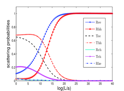
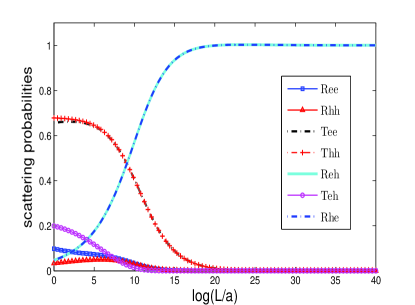
Figure 4: Typical RG flows of various scattering probabilities for two wires meeting at a junction with a $p$-wave superconducting region. Figure (a) shows the case with all $\alpha_{j}=0.2$, while (b) shows the case with all $\alpha_{j}=-0.2$.

We first discuss a two-wire problem as a guide to the more complicated three-wire problem. Here we have two NM wires with a SC region present at their junction. Then $S$ is a $4\times 4$ matrix of the form

$$S=\left(\begin{array}[]{cccc}r_{ee}&t_{ee}&r_{eh}&t_{eh}\\ t_{ee}&r_{ee}&t_{eh}&r_{eh}\\ r_{he}&t_{he}&r_{hh}&t_{hh}\\ t_{he}&r_{he}&t_{hh}&r_{hh}\end{array}\right).$$ (102)

(The condition $S^{T}=\tau^{z}S\tau^{z}$ implies that $r_{he}=-r_{eh}$ and $t_{he}=-t_{eh}$). Here we have assumed for simplicity that all the scattering amplitudes are the same for wires 1 and 2, for instance, $r_{ee,11}=r_{ee,22}$ and so on; these amplitudes can be complex in general. We will also assume that the interactions parameters are equal on the two wires, $\alpha_{1}=\alpha_{2}$.

We will first list the fixed points that we have found analytically for $S$-matrices of the form in Eq. (102). We will present the values of all the reflection and transmission amplitudes, with the understanding that two fixed points in which the amplitudes only differ by some phases as discussed in Eq. (98) will not be considered as different fixed points. We have found the following fixed points which are similar to the ones found for a junction with a $s$-wave superconductor in Ref. saha, .

(i) $r_{ee}=r_{hh}=1$, and all the other amplitudes are zero.

(ii) $r_{eh}=-r_{he}=1$, and all the other amplitudes are zero.

(iii) $t_{ee}=t_{hh}=1$, and all the other amplitudes are zero.

(iv) $t_{eh}=-t_{he}=1$, and all the other amplitudes are zero.

(v) $r_{ee}=t_{hh}=r_{he}=t_{he}=1/2$, and $t_{ee}=r_{hh}=r_{eh}=t_{eh}=-1/2$.

(vi) $t_{ee}=t_{hh}=\cos\theta$, $t_{eh}=-t_{he}=\sin\theta$, and all the other amplitudes are zero. Here $\theta$ can be any real number from 0 to $2\pi$. We thus have a continuous family of fixed points labeled by $\theta$. This is in contrast to the fixed points (i), (ii) and (v) given above which are all discrete fixed points. We note that the fixed points in (iii) and (iv) are special cases of (vi) corresponding to $\theta=0$ and $\pi/2$ respectively.

A simple way of finding fixed points analytically is to set all the reflection amplitudes equal to zero, $r_{ee,jj}=r_{hh,jj}=r_{eh,jj}=r_{he,jj}=0$. Then the matrix $F$ in Eq. (96) vanishes, and Eq. (97) straightaway gives $dS/dl=0$. All the other amplitudes in $S$ are then constrained by unitarity. This is how the family of fixed points in (vi) was found.

We will now numerically study the fixed points and their stabilities for Eq. (102). We begin by randomly generating a matrix $A$ satisfying the conditions $A^{\dagger}=A$ and $A^{T}=\tau^{z}A\tau^{z}$. Given an $A$, we construct $S=\exp(iA)$, and then use Eq. (97) to evolve $S$. In Figs. 4 (a) and (b), we show the typical RG flows of a number of reflection and transmission probabilities, such as $R_{ee}=|r_{ee}|^{2}$, $R_{hh}=|r_{hh}|^{2}$, etc. We find numerically that for a general starting point, $S$ always flows to the same fixed point which is described below. (By a general starting point, we mean that we do not start precisely at a special set of matrices which constitute some other fixed points which are not completely stable). For the case where $\alpha_{1}=\alpha_{2}=0.2$ (i.e., the interactions are repulsive), the plots in Fig. 4 (a) show that $S$ flows to a fixed point where $R_{ee}=R_{hh}=1$, and all the other probabilities are zero. If we start the RG evolution exactly at this point, $S$ does not flow at all and remains at that point. Hence this is the fixed point in the case of repulsive interactions. This is a completely stable fixed point because the RG flows always approach this fixed point independent of the $S$ that we start from; further, if we deviate a little bit in any direction from this fixed point, the RG flows take us back to the fixed point.

Interestingly, we find even if none of the symmetries are present, namely, $\alpha_{1}\neq\alpha_{2}$ (but both are positive), there is no time reversal symmetry ($S^{T}\neq\tau^{z}S\tau^{z}$), and the starting $S$-matrix is not symmetric between the two wires, $S$ always flows to a completely stable fixed point which is symmetric. More carefully speaking, one finds at the fixed point that although the phases of $r_{ee,jj}$ and $r_{hh,jj}$ are generally not equal to each other (the phases depend on the starting value of $S$ and the values of $\alpha_{j}$), all their magnitudes are equal to 1. We thus have a symmetry restoration at the fixed point.

For the opposite case in which $\alpha_{1}=\alpha_{2}=-0.2$ (i.e., attractive interactions), the plots in Fig. 4 (b) show that $S$ generally flows to a different fixed point where $R_{eh}=R_{he}=1$, and all the other probabilities are zero. This is the completely stable fixed point in this case as we always reach this point no matter where we start (unless again we start precisely at some special set of matrices which are fixed points which are not completely stable), and small deviations from this fixed point in any direction also flow to zero. Once again, we find that the phases of $r_{eh,jj}$ and $r_{he,jj}$ are generally not equal to each other but all their magnitudes are equal to 1 at the fixed point, even if there is no symmetry in the starting value of $S$ and of the $\alpha_{j}$ (provided that they are both negative).

We now observe that since Eq. (97) is linear in the $\alpha_{j}$, the equation depends only on the combination $\alpha_{j}l$. Hence the direction of the RG flows for $\alpha_{j}>0$ and $l\to\infty$ is just the opposite of the flows for $\alpha_{j}<0$ and $l\to\infty$. We therefore conclude that the stable fixed points for attractive interactions are exactly the same as the unstable fixed points for repulsive interactions. So the fixed point with $R_{eh}=R_{he}=1$ is the completely unstable fixed point for repulsive interactions, i.e., if we start slightly away from this point in any direction, the RG flows will always take us further away from the point.

We note that this numerical way of finding fixed points cannot detect fixed points which are partially stable and partially unstable, namely, stable in some directions and unstable in other directions. If we start near such a fixed point, we will generally always flow away from it regardless of whether we take all the $\alpha_{j}$ to be positive or negative.

Finally, let us discuss the RG fixed points and their stabilities for the three-wire problem. We again assume for simplicity that there is complete symmetry between the three wires, both in the $S$-matrix and the interactions strengths. $S$ is therefore a $6\times 6$ matrix of the form

$$S=\left(\begin{array}[]{cccccc}r_{ee}&t_{ee}&t_{ee}&r_{eh}&t_{eh}&t_{eh}\\ t_{ee}&r_{ee}&t_{ee}&t_{eh}&r_{eh}&t_{eh}\\ t_{ee}&t_{ee}&r_{ee}&t_{eh}&t_{eh}&r_{eh}\\ r_{he}&t_{he}&t_{he}&r_{hh}&t_{hh}&t_{hh}\\ t_{he}&r_{he}&t_{he}&t_{hh}&r_{hh}&t_{hh}\\ t_{he}&t_{he}&r_{he}&t_{hh}&t_{hh}&r_{hh}\end{array}\right).$$ (103)

We now present the results we find numerically, by starting with a randomly chosen matrix $S=\exp(iA)$ which has all the desired symmetries and then evolving it using Eq. (97). The typical RG flows of the various scattering probabilities are very similar to the ones shown for a two-wire system in Figs. 4 (a) and (b) for all the $\alpha_{j}$ equal to $0.2$ (repulsive) and $-0.2$ (attractive interactions) respectively. We see that the completely stable fixed point for repulsive interactions is again given by $R_{ee}=R_{hh}=1$, and all the other probabilities are zero. As we discussed above, the stable fixed points for attractive interactions, i.e., $\alpha_{j}<0$, are the unstable fixed points for repulsive interactions. Using this property we find that the completely stable fixed point for attractive interactions, and therefore the completely unstable fixed point for repulsive interactions, is given by $R_{eh}=R_{he}=1$, and all the other probabilities are zero. All these statements remain true even if the $\alpha_{j}$ are not equal to each other (although they must all have the same sign) and even if the starting value of $S$ has no symmetries. Thus the completely stable and completely unstable fixed points are similar for the two-wire and three-wire systems.

Before ending this section, we would like to mention the work done in Ref. affleck, on a junction of a superconducting wire and two non-superconducting wires where there are interactions. A non-trivial stable fixed point was found there which has perfect normal reflection for one linear combination of the electron fields in the two wires and perfect Andreev reflection for the other linear combination. This fixed point occurs because Ref. affleck, considers an interaction between the wires which mixes the two electron fields. We have not considered such inter-wire interactions in our model and therefore do not find such a non-trivial fixed point.

6.2  Conductances under RG flows

We will now use our understanding of the RG flows to study the conductances of a three-wire system as functions of physical parameters such as the wire lengths and the temperature, for the case of repulsive interactions. In particular, we will study how the conductances scale with various lengths when we approach the completely stable fixed point.

Using the procedure described in Eqs. (100) and (101), we first find the values of $\beta$ for different flow directions given by the perturbation $S_{1}$ around a fixed point $S_{0}$. The stable fixed point that we are interested in has only the $r_{ee,jj}$’s and $r_{hh,jj}$’s (namely, the diagonal elements of $S_{0}$) being unimodular numbers and all the other elements being zero. For a flow direction $S_{1}$ in which only the phases of the diagonal elements are changed, we find that $d\epsilon/dl=0$. This implies that $\beta=0$ and the RG flow is marginal. This is expected since the RG fixed points are invariant under multiplication by a diagonal unitary matrix as discussed in Eq. (98); hence there is no RG flow in those directions. Next, we look at the RG flows when only the $r_{eh,jj}$’s and $r_{he,jj}$’s are perturbed from zero. For this perturbation, we find that $d\epsilon/dl=-2\alpha\epsilon$; hence $\beta=-2\alpha$, and the RG flow in this direction is irrelevant. We choose $S_{1}$ where either (i) only the $t_{ee,ij}$’s and $t_{hh,ij}$’s are non-zero, or (ii) only the $t_{eh,ij}$’s and $t_{he,ji}$’s are non-zero. For both these cases we find that $d\epsilon/dl=-\alpha\epsilon$, which means that $\beta=-\alpha$ and the RG flows in these directions is also irrelevant. The RG flows near the fixed point $S_{0}$ are therefore either marginal or irrelevant in all directions.

Now we will discuss how the Cooper conductance $G_{C}$ and the normal conductances $G_{N2}$ and $G_{N3}$ scale under the RG flows (we are assuming that an electron is incident from the NM lead 1). Physically there are three length scales in the problem and we have to stop the RG flows when we reach the smallest of the three scales. One length scale is $\eta=\hbar v_{F}/\Delta$ which is associated with the SC gap, another is the wire length $L_{w}$ (we will take the lengths of all the three wires to be of the order of $L_{w}$), and the third scale is the thermal coherence length $L_{T}=\hbar v_{F}/(k_{B}T)$ if the system is at a temperature $T$ lal ; das2 . (We assume that all these length scales are much larger than the short distance scale $a$). We will now consider different regimes of these length scales.

(i) We first consider the case in which $L_{w}$ is finite and smaller than $\eta$, while $T\longrightarrow 0$ so that $L_{T}\longrightarrow\infty$. Then the length scale where the RG flows must be stopped is $L_{w}$. For a general perturbation around the stable fixed point, we have $|r_{he}|^{2}\sim e^{-4\alpha l}$, $|t_{he}|^{2}\sim e^{-2\alpha l}$, and $|t_{ee}|^{2}\sim e^{-2\alpha l}$, where $l=ln(L_{w}/a)$. We then find that $G_{C}=2(|r_{he}|^{2}+2|t_{he}|^{2})$ scales as

$$G_{C} \sim c_{1}e^{-4\alpha l}~{}+~{}c_{2}e^{-2\alpha l}$$ (104)

$$\sim \frac{c_{1}}{(L_{w}/a)^{4\alpha}}~{}+~{}\frac{c_{2}}{(L_{w}/a)^{2\alpha}},$$

where $c_{1},~{}c_{2}$ are some constants which depend on how far from the stable fixed point we are at the length scale $a$ where the RG flows begin. If $L_{w}\gg a$, the second term in Eq. (104) dominates over the first term. We therefore obtain

$$G_{C}~{}\sim~{}\frac{1}{(L_{w}/a)^{2\alpha}}.$$ (105)

Similarly we find that $G_{N2},~{}G_{N3}\sim|t_{ee}|^{2}-|t_{he}|^{2}$ scale as

$$G_{N2},~{}G_{N3}~{}\sim~{}\frac{1}{(L_{w}/a)^{2\alpha}}.$$ (106)

(ii) Next we consider the case in which $T$ is finite such that $L_{T}=\hbar v_{F}/(k_{B}T)$ is smaller than $\eta$, and $L_{w}\longrightarrow\infty$. Then the RG flows stop at the length scale $L_{T}$. Hence the elements of $S$ must be evaluated at $l=ln(L_{T}/a)=ln(v_{F}/(k_{B}Ta))$. Hence

$$G_{C}~{}\sim~{}c_{1}(k_{B}Ta/\hbar v_{F})^{4\alpha}~{}+~{}c_{2}(k_{B}Ta/\hbar v_{F})^{2\alpha}.$$ (107)

In the limit $k_{B}Ta/\hbar v_{F}\ll 1$, the second term dominates over the first and we get

$$G_{C}~{}\sim~{}(k_{B}Ta/\hbar v_{F})^{2\alpha}.$$ (108)

Similarly, we find

$$G_{N2},~{}G_{N3}~{}\sim~{}(k_{B}Ta/\hbar v_{F})^{2\alpha}.$$ (109)

(iii) Finally we consider the case where $\eta=\hbar v_{F}/\Delta$ is smaller than both $L_{w}$ and $L_{T}$. Then the RG flows must be stopped at the length scale $\eta$ since our RG equations were derived under the condition that the energy scale is much larger then $\Delta$. We then obtain expressions for the conductances which are similar to Eqs. (105) and (106) but with $L_{W}$ replaced by $\eta$.

To conclude, we see that the conductances $G_{C}$ and $G_{Nj}$ approach zero as powers of the smallest length of the system which may be $L_{w}$, $L_{T}$ or $\eta$. The exponents of the power laws can give an estimate of the strength of the interactions in the wires.

7  Experimental realization of systems with different signs of $\Delta_{j}$

We will now discuss how it may be possible to experimentally realize a system of three SC wires with the same or different signs of the $p$-wave pairings $\Delta_{j}$. We consider the system studied in Ref. ganga, . This consists of a wire with a Rashba spin-orbit coupling of the form $\pm\alpha_{R}p_{r}\sigma^{x}$, where $p_{r}$ is the momentum along the wire and $\sigma^{x}$ is a Pauli spin matrix. This form can arise as follows. Let us take the coordinate in the wire to increase along an arbitrary direction $\hat{r}$ lying in the $x-y$ plane. If the Rashba term is $\alpha_{R}{\hat{n}}\cdot{\vec{\sigma}}\times{\vec{p}}$, and $\hat{n}$ points in the $\hat{z}$ direction, then the Rashba term will be $\alpha_{R}p_{r}\sigma^{x}$ if ${\hat{r}}={\hat{y}}$ and $-\alpha_{R}p_{r}\sigma^{x}$ if ${\hat{r}}=-{\hat{y}}$.

Next, we place the wire in a magnetic field in the $\hat{z}$ direction which is perpendicular to the Rashba term (and has a Zeeman coupling $\Delta_{Z}$ to the spin of the electrons) and in proximity to a bulk $s$-wave SC with pairing $\Delta_{S}$. The complete Hamiltonian is ganga

$$H = \int dr~{}\Psi^{\dagger}_{\alpha}\left[(\frac{p_{r}^{2}}{2m}-\mu)\delta_{\alpha\beta}\pm\alpha_{R}p_{r}\sigma^{x}_{\alpha\beta}-\Delta_{Z}\sigma^{z}_{\alpha\beta}\right]\Psi_{\beta}$$ (110)

$$+\frac{i}{2}\int dr~{}[\Delta_{S}\Psi^{\dagger}_{\alpha}\sigma^{y}_{\alpha\beta}\Psi^{\dagger}_{\beta}+H.c.],$$

where $\Psi_{\alpha}$ is the annihilation operator for an electron with spin $\alpha$, and the $\pm$ sign of the Rashba term depends on whether ${\hat{r}}=\pm{\hat{y}}$. Ref.  ganga, then shows that for a certain range of the parameters, this system is equivalent to a spinless $p$-wave SC of the form that we have studied in this paper, with the $p$-wave pairing term being given by $-i(\Delta/k_{F})(c^{\dagger}\partial_{x}d+d^{\dagger}\partial_{x}c)$ (see Eq. (1)), where

$$\Delta~{}=~{}\pm~{}\frac{\alpha_{R}k_{F}\Delta_{S}}{\Delta_{Z}}.$$ (111)

Now consider a case in which the coordinates are given by ${\hat{r}}={\hat{y}}$ in all the three wires; see Fig. 5 (a). (The region where the three SC wires meet is an extended vertical region on the left side of the figure). Then the Rashba term and hence $\Delta_{j}$ will have the same sign in all the SC wires. On the other hand, suppose that one of the SC wires runs in a direction which is opposite to the other two wires as shown in Fig. 5 (b). (The three SC wires now meet along an extended vertical region in the middle of the figure). Now ${\hat{r}}=-{\hat{y}}$ in that wire while ${\hat{r}}={\hat{y}}$ in the other two wires. Then Eq. (111) shows that $\Delta_{j}$ will have one sign in that wire and the opposite sign in the other two wires.

[We would like to note that if the angle between the wires is different from zero or $\pi$, the situation will be more complicated because the Rashba term $\alpha_{R}{\hat{n}}\cdot{\vec{\sigma}}\times{\vec{p}}$ will no longer be proportional to the same $\vec{\sigma}$ matrix in the different wires. Hence the effective $p$-wave pairings in the different wires will not be related simply by sign changes in $\Delta_{j}$].

It is clear that the vertical region where the three SC wires meet is likely to cause some scattering of the electrons; we have modeled this scattering in the earlier sections using the matrix $\bf M$. Finally, the ends of the SC are connected to NM leads through tunnel barriers. As discussed in Sect. 2, these barriers can be characterized by their strength $\lambda$.

In Sects. 2 - 4, we discussed a conductance $G_{C}$ in which pairs of electrons can appear in (or disappear from) the SC regions. At a microscopic level we can understand these processes as occurring due to a Cooper pair going from the bulk $s$-wave SC to one of the $p$-wave SC wires (or vice versa). Finally we assume that the $s$-wave SC is grounded, and the three NM leads and the $s$-wave SC form a closed electrical circuit so that we can measure the conductances $G_{C}$ and $G_{Nj}$.

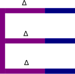
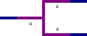
Figure 5: Three SC wires with (a) the sign of $\Delta_{j}$ being the same in all the wires, (b) the sign of $\Delta_{j}$ being different in the wire on the left compared to the other two wires. The SC wires are shown in a lighter shade while the NM leads are shown in a darker shade.

8  Conclusions

In this paper, we have studied the conductances of a system consisting of three $p$-wave superconductors, each connected to a normal metal lead (these are labeled as SC1, SC2, SC3 and NM1, NM2, NM3 respectively) in two different regimes of the energy. In Sects. 2 - 4, we have studied the Majorana and related sub-gap modes and their effects on the sub-gap conductances. Here we have considered two cases: (i) when the $p$-wave pair potentials $\Delta_{j}$ have the same sign in all the SCs, and (ii) when one of the $\Delta_{j}$ has a different sign from the other two. In Sects. 5 - 6, we have studied the effect of interactions between the electrons on the conductances at energies lying far from the SC gap.

To study the sub-gap modes, we have used a continuum model and current conservation to derive the boundary conditions at the junctions between the NMs and the SCs. Then we have found the boundary condition at the junction of the three SCs; this condition is encoded by a Hermitian matrix $\bf M$. Using these conditions, we have numerically studied two conductances, the Cooper pair conductance $G_{C}$ (from NM1 to the SCs) and the normal conductance $G_{N2}$ (from NM1 to NM2) when we send in an electron from NM1 with an energy $E$; we have taken $E$ to lie inside the superconducting gap so as to specifically probe the sub-gap modes which reduce to zero energy Majorana modes in the limit of long wire lengths.

We have looked at three different regimes of the lengths of the SCs with respect to $\eta$ which is the length scale associated with the SC gap. We find a rich pattern of the conductances as functions of the SC lengths and $E$.

We first consider the case when all the $\Delta_{j}$’s have the same sign. In the length regime $L\simeq\eta$ we find six sub-gap modes; these are not at zero energy because they hybridize with each other due to the finite lengths of the SCs. Among the six modes, three sit near the SC-NM junctions, and the other three sit at the junction of the three SCs. All these modes have a significant effect on the conductances and the latter shows peaks exactly at the energies of the sub-gap modes.

For the length regime $L\simeq 2\eta$ the hybridization among the sub-gap modes is less than in the previous case; hence the energy splitting of the sub-gap modes is also less. Even if we cannot clearly see six separate sub-gap modes, we can still observe several modes at non-zero energies.

In the third regime, when $L\gg\eta$, we find that the sub-gap modes are almost decoupled from each other and hence lie at zero energy. The Cooper conductance $G_{C}$ almost approaches its highest value of $2e^{2}/h$.

We compare our conductance results with the sub-gap energies that we get for a box made of three SC wires with hard walls (namely, without the NM leads). We generate plots for the energies of the sub-gap modes in all the three length regimes as discussed earlier. In the first length regime, instead of six sub-gap modes we see only four clearly; we believe this is due to the fact that two of the modes are very close to $E/\Delta=\pm 1$ and hence lie beyond our resolution. In the other two regimes, the plots of the energies of sub-gap modes almost exactly match with the conductance plots for the full system as we can see in Fig. 2.

In obtaining all these results, we have made a particular choice of the matrix $\bf M$ which defines the boundary condition at the junction of three SCs, namely, we have taken all the diagonal and off-diagonal elements of $\bf M$ to be equal to 1. If we take the elements to be different, the results may be somewhat different from what we get.

With the same choice of $\bf M$, we have calculated the conductances taking the $\Delta$ in SC1 to have a different sign compared to the $\Delta$’s in SC2 and SC3. The results are significantly different from the case of all $\Delta_{j}$’s having the same sign. In the length regime $L\simeq\eta$ we find four sub-gap modes at different energies, instead of six. Now there is only one sub-gap mode sitting at the junction of three SCs. As we increase $L/\eta$, the energy splitting between the sub-gap modes decreases; when $L\gg\eta$ we find that all the modes lie at zero energy. Once again we have compared our conductance results with the energies of the sub-gap modes in a SC box with the $\Delta$ in SC1 having an opposite sign to SC2 and SC3. The results match very well as we can see in Fig. 3.

We have then presented some analytical and symmetry arguments to explain the presence of multiple zero energy Majorana modes at a junction of three long SCs. Using the boundary condition at the junction we find that the number of independent variables in the problem directly corresponds to the number of Majorana modes at the junction. We have also used an “effective time reversal symmetry” to argue that the number of Majorana modes at a junction of three Kitaev chains can be either one or three.

Next, we have studied the effect of interactions between the electrons in order to understand the conductances at energies far from the SC gap. (We emphasize that the energy range we have considered is different from earlier work where RG equations have been studied at energies within or close to the SC gap, where the various reflection and transmission amplitudes vary rapidly with the energy fidkowski2 ; titov ). We have derived the RG equations for a general scattering matrix $S$ which governs a system of several NM wires which meet at a junction with a SC region. The RG flows of the elements of $S$ are entirely a result of the interactions in the NM wires; there is no flow if all the interaction parameters $\alpha_{j}$ are equal to zero. We have found stable and unstable fixed points for two-wire and three-wire junctions when the interactions are repulsive, i.e., $\alpha_{j}>0$. A completely stable fixed point is one where the RG flows take us back to the fixed point for a small deviation from it in any direction. We find that at the completely stable fixed point, the magnitudes of all the normal reflection probabilities are equal to 1, while at the completely unstable fixed points all the Andreev reflection probabilities are equal to 1. We have discussed the consequences of the RG flows on the conductances of the system, assuming all the interaction parameters to be equal to $\alpha$. A stability analysis near the stable fixed point shows that when the wire lengths $L_{w}$ are finite and the temperature $T\longrightarrow 0$, the Cooper conductance $G_{C}$ and the normal conductances $G_{N2},~{}G_{N3}$ all scale as $1/L_{w}^{2\alpha}$. In the other limit where $T$ is finite (but small compared to the band width of the system), and $L_{w}\longrightarrow\infty$, $G_{C}$, $G_{N2}$ and $G_{N3}$ scale as $T^{2\alpha}$. In general, for an electron incident from NM lead $j$, the conductance measured on NM lead $j$ will scale as $1/L_{w}^{2\alpha}$ or $T^{2\alpha}$ depending on which length scale is smaller. Thus a measurement of the conductances can provide valuable information about the strength of the interactions between the electrons.

We can summarize our most important results as follows.

(i) We have shown that a system of three $p$-wave SC wires with NM leads has multiple sub-gap modes and all these modes contribute to peaks in the conductance; the positions of the peaks exactly match the energies of the sub-gap modes. We thus have a novel system with a large number of sub-gap conductance peaks which vary with the applied bias and wire lengths in an interesting way.

(ii) To study the conductances far from the SC gap, we have used an RG method which directly uses the fermionic language to look at the effect of interactions on the scattering matrix. (This is in contrast to earlier RG studies of $p$-wave superconductors which used bosonization and studied the RG flows of parameters in the bosonic Hamiltonian rather than the scattering matrix). We have shown that interactions make the scattering matrix flow to certain stable fixed points at large wire lengths and low temperatures. The fixed points are symmetric under permutations of the wires and under time reversal even if the system does not have these symmetries at the microscopic length scale. Near the stable fixed point, we have shown that the conductances scale as a power of the wire length or the temperature, and the power can give us an estimate of the strength of the interactions.

Putting the above results together, we get a complete picture of the conductances of a system of three $p$-wave SC wires both inside and far outside the SC gap.

Finally, we have discussed how our model can be experimentally implemented by taking three wires with Rashba spin-orbit coupling, applying a Zeeman field perpendicular to the direction of the Rashba field, and placing the system in proximity to an $s$-wave superconductor. In a particular range of parameters, each wire effectively becomes a $p$-wave SC. The cases where the three SC wires have the same sign of the $p$-wave pairing or one of them has the opposite sign of the pairing can both be implemented, simply by rearranging the orientation of one of the wires. As we have shown in the earlier sections, the number of sub-gap modes is different in the two cases, and this leads to a significant difference in the pattern of conductance peaks as a function of the energy and wire lengths. In future, we can generalize our studies of a single three-wire junction to more complicated systems such as networks of wires forming a lattice alicea1 ; zhou , where each vertex of the lattice can host one or more sub-gap modes.

References

- (1)
- (2) C. W. J. Beenakker, Annu. Rev. Condens. Matter Phys. 4, 113 (2013)
- (3) C. Nayak, S. H. Simon, A. Stern, M. Freedman, and S. Das Sarma, Rev. Mod. Phys. 80, 1083 (2008)
- (4) A. Kitaev, Physics-Uspekhi 44, 131 (2001)
- (5) R. M. Lutchyn, J. D. Sau, and S. Das Sarma, Phys. Rev. Lett. 105, 077001 (2010); Y. Oreg, G. Refael, and F. von Oppen, Phys. Rev. Lett. 105, 177002 (2010)
- (6) L. Fu, Phys. Rev. Lett. 104, 056402 (2010).
- (7) A. C. Potter and P. A. Lee, Phys. Rev. Lett. 105, 227003 (2010); K. T. Law and P. A. Lee, Phys. Rev. B 84, 081304(R) (2011)
- (8) V. Shivamoggi, G. Refael, and J. E. Moore. Phys. Rev. B 82, 041405(R) (2010)
- (9) D. Sen and S. Vishveshwara, EPL 91, 66009 (2010); W. DeGottardi, D. Sen, and S. Vishveshwara, New. J. Phys. 13, 065028 (2011)
- (10) L. Fidkowski and A. Kitaev, Phys. Rev. B 83, 075103 (2011)
- (11) P. W. Brouwer, M. Duckheim, A. Romito, and F. von Oppen, Phys. Rev. Lett. 107, 196804 (2011), and Phys. Rev. B 84, 144526 (2011)
- (12) J. Alicea, Y. Oreg, G. Refael, F. von Oppen, and M. P. A. Fisher, Nature Phys. 7, 412 (2011)
- (13) I. C. Fulga, F. Hassler, A. R. Akhmerov, and C. W. J. Beenakker, Phys. Rev. B 83, 155429 (2011); A. R. Akhmerov, J. P. Dahlhaus, F. Hassler, M. Wimmer, and C. W. J. Beenakker, Phys. Rev. Lett. 106, 057001 (2011)
- (14) T. D. Stanescu, R. M. Lutchyn, and S. Das Sarma, Phys. Rev. B 84, 144522 (2011); T. D. Stanescu, S. Tewari, J. D. Sau, and S. Das Sarma, Phys. Rev. Lett. 109, 266402 (2012); T. D. Stanescu and S. Tewari, J. Phys. Condens. Matter 25, 233201 (2013); T. D. Stanescu and S. Tewari, Phys. Rev. B 89, 220507(R) (2014); S. Das Sarma, J. D. Sau, and T. D. Stanescu, Phys. Rev. B 86, 220506(R) (2012)
- (15) S. Gangadharaiah, B. Braunecker, P. Simon, and D. Loss, Phys. Rev. Lett. 107, 036801 (2011)
- (16) E. M. Stoudenmire, J. Alicea, O. A. Starykh, and M. P. A. Fisher, Phys. Rev. B 84, 014503 (2011); R. M. Lutchyn and M. P. A. Fisher, Phys. Rev. B 84, 214528 (2011)
- (17) L. Fidkowski, J. Alicea, N. H. Lindner, R. M. Lutchyn, and M. P. A. Fisher, Phys. Rev. B 85, 245121 (2012)
- (18) S. B. Chung, H.-J. Zhang, X.-L. Qi, and S.-C. Zhang, Phys. Rev. B 84, 060510 (2011)
- (19) E. Sela, A. Altland, and A. Rosch, Phys. Rev. B 84, 085114 (2011)
- (20) L. Jiang, T. Kitagawa, J. Alicea, A. R. Akhmerov, D. Pekker, G. Refael, J. I. Cirac, E. Demler, M. D. Lukin, and P. Zoller, Phys. Rev. Lett. 106, 220402 (2011)
- (21) T. Dirks, T. L. Hughes, S. Lal, B. Uchoa, Y.-F. Chen, C. Chialvo, P. M. Goldbart, and N. Mason, Nature Phys. 7, 386 (2011)
- (22) S. Tewari and J. D. Sau, Phys. Rev. Lett. 109, 150408 (2012); E. Dumitrescu, B. Roberts, S. Tewari, J. D. Sau, and S. Das Sarma, Phys. Rev. B 91, 094505 (2015); E. Dumitrescu, G. Sharma, J. D. Sau, and S. Tewari, Phys. Rev. B 92, 045421 (2015)
- (23) B. Beri and N. R. Cooper, Phys. Rev. Lett. 109, 156803 (2012)
- (24) M. Gibertini, F. Taddei, M. Polini, and R. Fazio, Phys. Rev. B 85, 144525 (2012); J. S. Lim, L. Serra, R. López, and R. Aguado, Phys. Rev. B 86, 121103 (2012); M. Tezuka and N. Kawakami, Phys. Rev. B 85, 140508(R) (2012); R. Egger and K. Flensberg, Phys. Rev. B 85, 235462 (2012)
- (25) A. M. Lobos, R. M. Lutchyn, and S. Das Sarma, Phys. Rev. Lett. 109, 146403 (2012)
- (26) R. Hützen, A. Zazunov, B. Braunecker, A. Levy Yeyati, and R. Egger, Phys. Rev. Lett. 109, 166403 (2012)
- (27) F. Pientka, G. Kells, A. Romito, P. W. Brouwer, and F. von Oppen, Phys. Rev. Lett. 109, 227006 (2012); F. Pientka, A. Romito, M. Duckheim, Y. Oreg, and F. von Oppen, New J. Phys. 15, 025001 (2013)
- (28) D. Roy, C. J. Bolech, and N. Shah, Phys. Rev. B 86, 094503 (2012), and arXiv:1303.7036
- (29) A. M. Cook, M. M. Vazifeh, and M. Franz, Phys. Rev. B 86, 155431 (2012); F. L. Pedrocchi, S. Chesi, S. Gangadharaiah, and D. Loss, Phys. Rev. B 86, 205412 (2012)
- (30) D. Sticlet, C. Bena, and P. Simon, Phys. Rev. Lett. 108, 096802 (2012); D. Chevallier, D. Sticlet, P. Simon, and C. Bena, Phys. Rev. B 85, 235307 (2012); D. Chevallier, D. Sticlet, P. Simon, and C. Bena, Phys. Rev. B 87, 165414 (2013); I. Martin and A. F. Morpurgo, Phys. Rev. B 85, 144505 (2012)
- (31) P. San-Jose, E. Prada, and R. Aguado, Phys. Rev. Lett. 108, 257001 (2012); E. Prada, P. San-Jose, and R. Aguado, Phys. Rev. B 86, 180503 (2012)
- (32) J. Klinovaja and D. Loss, Phys. Rev. B 86, 085408 (2012); D. Rainis, L. Trifunovic, J. Klinovaja, and D. Loss, Phys. Rev. B 87, 024515 (2013)
- (33) J. Alicea, Rep. Prog. Phys. 75, 076501 (2012)
- (34) F. Hassler and D. Schuricht, New J. Phys. 14, 125018 (2012)
- (35) J. D. Sau and S. Das Sarma, Nature Communications 3, 964 (2012); J. D. Sau, C. H. Lin, H.-Y. Hui, and S. Das Sarma, Phys. Rev. Lett. 108, 067001 (2012)
- (36) J. Liu, A. C. Potter, K. T. Law, and P. A. Lee, Phys. Rev. Lett. 109, 267002 (2012)
- (37) L.-J. Lang and S. Chen, Phys. Rev. B 86, 205135 (2012)
- (38) Y. Niu, S. B. Chung, C.-H. Hsu, I. Mandal, S. Raghu, and S. Chakravarty, Phys. Rev. B 85, 035110 (2012)
- (39) M. Leijnse and K. Flensberg, Semicond. Sci. Technol. 27, 124003 (2012)
- (40) S. Nadj-Perge, I. K. Drozdov, B. A. Bernevig, and A. Yazdani, Phys. Rev. B 88, 020407(R) (2013)
- (41) W. DeGottardi, D. Sen, and S. Vishveshwara, Phys. Rev. Lett. 110, 146404 (2013)
- (42) W. DeGottardi, M. Thakurathi, S. Vishveshwara, and D. Sen, Phys. Rev. B 88, 165111 (2013)
- (43) X. Cai, L.-J. Lang, S. Chen, and Y. Wang, Phys. Rev. Lett. 110, 176403 (2013)
- (44) A. Keselman, L. Fu, A. Stern, and E. Berg, Phys. Rev. Lett. 111, 116402 (2013); T. Ojanen, Phys. Rev. B 87, 100506(R) (2013); P. Lucignano, F. Tafuri, and A. Tagliacozzo, Phys. Rev. B 88, 184512 (2013)
- (45) J. Klinovaja, P. Stano, A. Yazdani, and D. Loss, Phys. Rev. Lett. 111, 186805 (2013)
- (46) I. Adagideli, M. Wimmer, and A. Teker, Phys. Rev. B 89, 144506 (2014)
- (47) A. Manolescu, D. C. Marinescu, and T. D. Stanescu, J. Phys. Condens. Matter 26, 172203 (2014)
- (48) A. M. Lobos and S. Das Sarma, New J. Phys. 17, 065010 (2015)
- (49) O. Kashuba and C. Timm, Phys. Rev. Lett. 114, 116801 (2015)
- (50) A. Ghazaryan and T. Chakraborty, Phys. Rev. B 92, 115138 (2015)
- (51) M. Guigou, N. Sedlmayr, J. M. Aguiar-Hualde, and C. Bena, arXiv:1407.1393v2
- (52) J. Klinovaja and D. Loss, Eur. Phys. J. B 88, 62 (2015)
- (53) R. J. Doornenbal, G. Skantzaris, and H. T. C. Stoof, Phys. Rev. B 91, 045419 (2015)
- (54) H.-C. Kao, Phys. Rev. B 90, 245435 (2014)
- (55) S. Hegde, V. Shivamoggi, S. Vishveshwara, and D. Sen, New J. Phys. 17, 053036 (2015)
- (56) M. Thakurathi, O. Deb, and D. Sen, J. Phys. Condens. Matter 27, 275702 (2015)
- (57) C. Spanslatt, E. Ardonne, J. C. Budich, and T. H. Hansson, J. Phys. Condens. Matter 27, 405701 (2015)
- (58) S. Das and I. I. Satija, arXiv:1409.6139; I. Mandal and S. Tewari, arXiv:1502.03110
- (59) V. Mourik, K. Zuo, S. M. Frolov, S. R. Plissard, E. P. A. M. Bakkers, and L. P. Kouwenhoven, Science 336, 1003 (2012)
- (60) M. T. Deng, C. L. Yu, G. Y. Huang, M. Larsson, P. Caroff, and H. Q. Xu, Nano Lett. 12, 6414 (2012)
- (61) A. Das, Y. Ronen, Y. Most, Y. Oreg, M. Heiblum, and H. Shtrikman, Nature Phys. 8, 887 (2012)
- (62) A. D. K. Finck, D. J. Van Harlingen, P. K. Mohseni, K. Jung, and X. Li, Phys. Rev. Lett. 110, 126406 (2013); A. D. K. Finck, C. Kurter, Y. S. Hor, and D. J. Van Harlingen, Phys. Rev. X 4, 041022 (2014)
- (63) E. J. H. Lee, X. Jiang, M. Houzet, R. Aguado, C. M. Lieber, and S. De Franceschi, Nature Nanotechnology 9, 79 (2014)
- (64) S. Nadj-Perge, I. K. Drozdov1, J. Li, H. Chen, S. Jeon, J. Seo, A. H. MacDonald, B. A. Bernevig, and A. Yazdani, Science 346, 602 (2014)
- (65) R. Pawlak, M. Kisiel, J. Klinovaja, T. Meier, S. Kawai, T. Glatzel, D. Loss, and E. Meyer, arXiv:1505.06078
- (66) L. P. Rokhinson, X. Liu, and J. K. Furdyna, Nature Phys. 8, 795 (2012)
- (67) Y. Zhou and M. W. Wu, J. Phys. Condens. Matter 26, 065801 (2014); L. Weithofer, P. Recher, and T. L. Schmidt, Phys. Rev. B 90, 205416 (2014); S. Valentini, R. Fazio, V. Giovannetti, and F. Taddei, Phys. Rev. B 91, 045430 (2015); F. L. Pedrocchi and D. P. DiVincenzo, Phys. Rev. Lett. 115, 120402 (2015)
- (68) A. M. Tsvelik, Phys. Rev. Lett. 110, 147202 (2013); N. Crampe and A. Trombettoni, Nucl. Phys. B 871, 526 (2013)
- (69) E. Eriksson, C. Mora, A. Zazunov, and R. Egger, Phys. Rev. Lett. 113, 076404 (2014); E. Eriksson, A. Nava, C. Mora, and R. Egger, Phys. Rev. B 90, 245417 (2014)
- (70) A. Altland and R. Egger, Phys. Rev. Lett. 110, 196401 (2013); A. Altland, B. Beri, R. Egger, and A. M. Tsvelik, Phys. Rev. Lett. 113, 076401 (2014); A. Zazunov, A. Altland, and R. Egger, New J. Phys. 16, 015010 (2014)
- (71) I. Affleck and D. Giuliano, J. Stat. Mech. (2013) P06011.
- (72) G. E. Blonder, M. Tinkham, and T. M. Klapwijk, Phys. Rev. B 25, 4515 (1982)
- (73) A. Kastalsky, A. W. Kleinsasser, L. H. Greene, R. Bhat, F. P. Milliken, and J. P. Harbison, Phys. Rev. Lett. 67, 3026 (1991); C.-R. Hu, Phys. Rev. Lett. 72 1526 (1994); J. Yang and C.-R. Hu, Phys. Rev. B 50, 16766 (1994); Y. Tanaka and S. Kashiwaya, Phys. Rev. Lett. 74, 3451 (1995)
- (74) K. Sengupta, I. Zutić, H.-J. Kwon, V. M. Yakovenko, and S. Das Sarma, Phys. Rev. B 63, 144531 (2001); K. Sengupta, H.-J. Kwon, and V. M. Yakovenko, Phys. Rev. B 65, 104504 (2002); H.-J. Kwon, K. Sengupta and V. M. Yakovenko, Eur. Phys. J. B 37, 349 (2004)
- (75) T. Yokoyama, Y. Tanaka, and J. Inoue, Phys. Rev. B 74, 035318 (2006); T. Yokoyama, Y. Tanaka, and N. Nagaosa, Phys. Rev. Lett. 102, 166801 (2009)
- (76) A. Hayat, P. Zareapour, S. Y. F. Zhao, A. Jain, I. G. Savelyev, M. Blumin, Z. Xu, A. Yang, G. D. Gu, H. E. Ruda, S. Jia, R. J. Cava, A. M. Steinberg, and K. S. Burch, Phys. Rev. X 2, 041019 (2012)
- (77) A. F. Andreev, Sov. Phys. JETP 19, 1228 (1964)
- (78) A. O. Gogolin, A. A. Nersesyan, and A. M. Tsvelik, Bosonization and Strongly Correlated Systems (Cambridge University Press, Cambridge, 1998); J. von Delft and H. Schoeller, Ann. Phys. (Leipzig) 7, 225 (1998); S. Rao and D. Sen, in Field theories in Condensed Matter Physics, edited by S. Rao (Hindustan Book Agency, New Delhi, 2001); T. Giamarchi, Quantum Physics in One Dimension (Oxford University Press, Oxford, 2004)
- (79) C. Nayak, M. P. A. Fisher, A. W. W. Ludwig, and H. H. Lin, Phys. Rev. B 59, 15694 (1999)
- (80) S. Chen, B. Trauzettel, and R. Egger, Phys. Rev. Lett. 89, 226404 (2002)
- (81) C. Chamon, M. Oshikawa, and I. Affleck, Phys. Rev. Lett. 91, 206403 (2003); M. Oshikawa, C. Chamon, and I. Affleck, J. Stat. Mech.: Theory Exp. (2006) P02008.
- (82) B. Bellazzini, M. Mintchev, and P. Sorba, J. Phys. A 40, 2485 (2007), and J. Math. Phys. 51, 032302 (2010); B. Bellazzini, M. Burrello, M. Mintchev, and P. Sorba, Proc. Symp. Pure Math. 77, 639 (2008)
- (83) A. Agarwal, S. Das, S. Rao, and D. Sen, Phys. Rev. Lett. 103, 026401 (2009), and Erratum, Phys. Rev. Lett. 103, 079903 (2009)
- (84) X. Barnabe-Theriault, A. Sedeki, V. Meden, and K. Schönhammer, Phys. Rev. Lett. 94, 136405 (2005); V. Meden, S. Andergassen, T. Enss, H. Schoeller, and K. Schönhammer, New J. Phys. 10, 045012 (2008)
- (85) D. Yue, L. I. Glazman, and K. A. Matveev, Phys. Rev. B 49, 1966 (1994); K. A. Matveev, D. Yue, and L. I. Glazman, Phys. Rev. Lett. 71, 3351 (1993)
- (86) S. Lal, S. Rao and D. Sen, Phys. Rev. B 66, 165327 (2002)
- (87) S. Das, S. Rao and D. Sen, Phys. Rev. B 70, 085318 (2004)
- (88) S. Das, S. Rao, and A. Saha, Phys. Rev. B 77, 155418 (2008), and Phys. Rev. B 79, 155416 (2009)
- (89) A. Soori, O. Deb, K. Sengupta, and D. Sen, Phys. Rev. B 87, 245435 (2013)
- (90) K. T. Law, P. A. Lee, and T. K. Ng, Phys. Rev. Lett. 103, 237001 (2009)
- (91) M. Titov, M. Müller, and W. Belzig, Phys. Rev. Lett. 97, 237006 (2006)
- (92) J. Solyom, Adv. Phys. 28, 201 (1979)