U(1) and SU(2) quantum dissipative systems: The Caldeira-Leggett vs. the Amegaokar-Eckern-Schön approaches
Abstract
There are two paradigmatic frameworks for treating quantum systems coupled to a dissipative environment: the Caldeira-Leggett and the Ambegaokar-Eckern-Schön approaches. Here we recall the differences between them, and explain the consequences when each is applied to a zero dimensional spin (possessing an SU(2) symmetry) in a dissipative environment (a dissipative quantum dot near or beyond the Stoner instability point).
The diagrammatic technique for non-equilibrium systems developed in the pioneering works of Schwinger and Keldysh plays a predominant role in theoretical condensed matter physics Schwinger61 ; Keldysh65 . It is designed to tackle real time evolution of systems at and away from equilibrium. Following the developments of the last two decades KamenevAndreev ; KamenevBook ; AltlandBook , it now provides a non-perturbative tool to tackle interaction induced strong correlations in quantum many-body systems. In this paper we discuss an important prototypical problem, a quantum zero dimensional degree of freedom in a dissipative environment, in which the Keldysh technique is of tremendous use, providing insight into the physics involved.
I General perspective
We consider here the dynamics of a quantum system coupled to a dissipative environment. The resulting equation-of-motion is stochastic, which can be formulated on any of the following three levels: (i) a fully classical Langevin equation, where both the variables are classical (expectation values of observables) and the frequency range of interest is . For Ohmic dissipation the noise spectrum is white; (ii) a semi-classical hybrid description, within which the variables are still classical coordinates, but one acknowledges the fact that the noise may be quantum, having high frequency component, (Ref. ASchmid82_Langevin ); (iii) a full-fledged quantum mechanical description, according to which the noise may contain high frequency quantum components, and the variables of the quantum Langevin equation are operators within the Heisenberg description. This approach is practiced, say, in the field of quantum optics GardinerZollerBook .
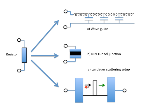
A paradigmatic framework to present a dissipative environment, in a way that connects to our preformed classical intuition, is to model Ohmic resistor quantum mechanically. We mention here three approaches:
1. The Caldeira-Leggett (CL) modelling CaldeiraLeggett81 : One introduces an effective circuit consisting of an L-C transmission line (with infinitesimal imaginary term), that may extract energy and current from the bare quantum system. (cf. Fig. 1a)
2. The Ambegaokar-Eckern-Schön (AES) modeling AES_PRL ; AES_PRB : Here we model a tunnel junction (cf. Fig. 1b) , assuming explicitly that its transparency is low, hence only lowest order contributions in the tunneling should be accounted for. The resulting Hamiltonian represents reservoir degrees of freedom that give rise to dissipation. Traditional applications of the CL picture employed extended coordinates (this, however, is not a must; the CL action in the case of a spin degree-of-freedom consists of compact coordinates). By contrast the AES approach introduces compact (periodic) coordinates.
3. The Landauer picture Landauer70 ; Buettiker86 ; ImryBook . Here one models the resistor by a tunnel barrier (of arbitrary transparency) (cf. Fig. 1c for the single channel case). The contribution of this tunnel barrier to the resistance is given by , where the reflection probability off the barrier is equal to the modulus square of the reflection amplitude, . This elastic backscattering process yields the magnitude of the resistor; the actual inelastic dissipation takes place in the connected reservoirs. Such a model has been discussed, for example, in Ref. NazarovBlanterBook . We shall not consider this picture here.
The outline of this paper is the following: in Section II we will briefly review earlier works, emphasizing the difference between the CL and AES approaches to dissipative dynamics, focusing on charge dynamics. The gauge symmetry underlying charge transport is U(1). In Section III we will recall the physics of a quantum dot (QD) tuned to be near (but below) the Stoner instability. As such, the QD supports large magnetization. Ignoring fluctuations in the magnitude of the spin, the spin degree of freedom possesses an SU(2) symmetry. The coupling of such a QD to external leads gives rise to dissipation, which is formulated and studied within the framework of the AES (Section IV). In Section V we first compare our AES analysis for the spin case to our results obtained within the CL framework. We then note that this AES vs. CL contrast differs from the AES vs. CL in the standard charge U(1) case. We conclude in Section VI.
II Caldeira-Leggett versus Ambegaokar-Eckern-Schön: the Charge U(1) Case
We consider the dynamics associated with current through a resistor, and compare the two paradigmatic representation thereof: CL and AES.
II.1 CL action
The CL action of a current biased linear resistor (modeled as a transmission line) reads
| (1) |
Here the dimensionless phase variable represents the effective flux variable via , where is the flux quantum. The voltage across the resistor is given by , and is the degree-of-freedom canonically conjugate to the charge that has flown through the resistor . In (1) is the kernel of the Ohmic bath CaldeiraLeggett81 . Dropping the time-local terms (important for avoiding renormalization of the non-dissipative part of the action) we obtain
| (2) |
Note that in Keldysh notation this action may be written as
| (8) | |||
| (9) |
where refer to the classical and quantum components on the Keldysh contour KamenevBook 111Unlike Ref. KamenevBook we use the convention , , where refer to the forward and the backward parts of the Keldysh contour respectively.. The subscripts refer to the retarded, advanced, and Keldysh components of the matrix.
Employing the relation between the retarded and the advanced components of the kernel , we may write the action as
| (10) |
with
| (11) |
| (12) |
and
| (13) |
One may ASchmid82_Langevin rewrite the Keldysh term of the action, employing the decoupling
| (14) |
It follows that
| (15) |
The resulting Langevin equation-of-motion is obtained by calculating the variation . The equation obtained is
| (16) |
where represents stochastic current noise. We note that the noise is additive, and is not affected by the bias current.
In deriving Eq. 16 we have used the fact that the dissipative bath has an Ohmic spectrum CaldeiraLeggett81 , implying that
| (17) |
where is the resistance. The variation over the retarded part of the action leads to
| (18) |
The Fourier transform of the current noise correlator is given by
| (19) |
At equilibrium
| (20) |
The fluctuation-dissipation theorem follows from Eqs. (18) and (20).
| (21) |
We note that the additivity of the noise and its independence of the bias current (Eq. 16) imply that the noise is independent of , i.e., absence of shot noise.
II.2 AES action
The AES action now is given by
| (22) |
The source term is the same as in the previous case. Similarly to the CL case, Eq. (10), one may write the action as
| (23) |
The retarded part is essentially identical to that in the CL case, having to do with the fact that and are very close to each other (cf. Eq. (17)), which allows us to expand the term in Eq. (22). The Keldysh term, though, is very different:
| (24) |
Decoupling the action, employing two auxiliary fields, and , one obtains AES_PRB
| (25) |
The resulting equation-of-motion for the AES action is
| (26) |
This equation can be cast into the form of Eq. (16) by writing with the two independent terms of current fluctuations defined as
| (27) |
The equation-of-motion (26) implies that the noise is non-additive, as can be shown explicitly from the following iterative procedure. The zeroth iteration gives , where . Next we introduce a correction and obtain
| (28) |
The first iteration consists in dropping in the r.h.s. of Eq. (28). The resulting stochastic terms give rise to shot noise AES_PRB (unlike the CL equation-of-motion). For we find
| (29) |
III A Quantum Dot near the Stoner Phase Transition
Over the past few decades the physics of quantum dots has become a focal point of research in nanoelectronics. The introduction of the ”Universal Hamiltonian“ PhysRevB.62.14886 ; AleinerBrouwerGlazman ; alhassidreview ; KamenevAndreev2 has made it possible to take into account the effects of electron-electron (e-e) interaction within a QD in a controlled way. This approach is applicable for a normal-metal QD when the Thouless energy and the mean single particle level spacing satisfy . Here is the dimensionless conductance of the QD. The single particle level spacing is given by , where is the volume of the QD and is its density of states (DoS) and therefore for a d-dimensional QD. The Thouless energy, , is the inverse time-of-flight (or diffusion time) of an electron across the quantum dot.
Within this scheme interactions are split into a sum of three spatially independent contributions in the charging, spin-exchange, and Cooper channels. Ignoring the latter (see below) the charging term leads to the phenomenon of Coulomb blockade, while the spin-exchange term can drive the system towards the Stoner instability Stoner . In bulk systems the exchange interaction competes with the kinetic energy leading to Stoner instability. In finite size systems mesoscopic Stoner regime may be a precursor of bulk thermodynamic Stoner instability PhysRevB.62.14886 ; AleinerBrouwerGlazman : a new phase, intermediate between paramagnetic and ferromagnetic emerges, in which the total spin of the QD is finite but not extensive (i.e., not proportional to the volume of the dot). The mesoscopic Stoner regime can be realized in QDs made of materials close to the thermodynamic Stoner instability.
A quantum dot in the metallic regime, , is described by the universal Hamiltonian PhysRevB.62.14886 :
| (30) |
The noninteracting part of the universal Hamiltonian reads
| (31) |
where denotes the energy of a spin-degenerate (index ) single particle level . The charging interaction term
| (32) |
accounts for the Coulomb blockade. Here, denotes the charging energy of the quantum dot with the self-capacitance , represents the background charge, and is the operator of the total number of electrons of the dot. For the isolated quantum dot the total number of electrons is fixed and, therefore, the charging interaction term can be omitted. The term
| (33) |
represents the ferromagnetic () exchange interaction within the dot where is the operator of the total spin of the dot. Here , where is a vector made of Pauli matrices. The interaction in the Cooper channel is described by
| (34) |
In what follows we do not take into account for the following reasons. For the dots defined in 2D electron gas the interaction in the Cooper channel is typically repulsive and, therefore, renormalizes to zero AleinerBrouwerGlazman . In the case of 3D quantum dots realized as small metallic grains, the interaction in the Cooper channel can be attractive, giving rise to interesting competition between superconductivity and ferromagnetism Schechter ; AlhassidSF1 ; AlhassidSF2 . In that case we assume that there is a weak magnetic field which suppresses the Cooper channel.
The starting point of our analysis of a dissipative Stoner QD (near the Stoner instability point) accounts for the QD Hamiltonian
| (35) |
In doing so we ignore possible correlations between the charging state and the spin configuration of the QD boazgefen .
We note that for isotropic spin exchange interaction (Heisenberg model) the mesoscopic Stoner phase extends over . For the anisotropic case PhysRevLett.96.066805 ; PhysRevB.90.195308 the lower boundary of this inequality slides towards 1, with no mesoscopic Stoner phase for Ising spin boazgefen ; PhysRevB.89.201304 . For the isotropic case the ground state spin S is the integer value (for even number of electrons on the QD) or half-integer value (for odd number) that is closest to . This value increases with increasing J and diverges for , which marks the onset of the macroscopic Stoner ferromagnetic phase. Seemingly the problem is easy to tackle theoretically. The interaction terms of the universal Hamiltonian consist only of zero mode (zero wave-number) contributions, which commute with each other. The inclusion of the exchange term renders the problem non-trivial though: the resulting action, which consists of Pauli matrices, is non-Abelian (more specifically, it is underlined by an SU(2) symmetry). Attempts to study the problem from different points of view included the Ising limit boazgefen , perturbation theory in the Ising anisotropy PhysRevLett.96.066805 . An exact solution that employs states classified by the total number of electrons and the total spin AlhassidRupp ; PhysRevB.69.115331 ; TureciAlhassid requires the calculation of Clebsch-Gordan coefficients which is not an easy task. In this way Alhassid and Rupp have found an exact solution for the partition function in the absence of Zeeman splitting. Elements of their analysis were then incorporated into a master equation analysis of electric AlhassidRupp ; PhysRevB.69.115331 and thermal PhysRevB.81.205303 properties. Independently, a study of electron transport through a QD for low temperatures () was made in reference UsajBaranger . That analysis, accounting for the charging and exchange interactions, employed a master equation approach as well.
An exact solution based on the Wei-Norman-Kolokolov approach had been presented in reference JETPLetters.92.179 , and was then extended to include randomness-induced spectral fluctuations PhysRevB.85.155311 . The tunneling density of states and the spin susceptibility were calculated; other thermodynamic and linear response correlations are calculable as well. The study of shot noise near the Stoner point was reported in SothmannKoenigGefen .
We note that the exact solution approaches mentioned above, while elegant and powerful, are very difficult to generalize to more complex setups, in particular, to setups where external leads are added – a common mean for the introduction of dissipation. An efficient approximation, which can be generalized to such setups, employs adiabatic approximation of the spin stochastic dynamics SahaAnnals .
IV AES approach for SU(2) spin
Our approach PhysRevLett.114.176806 can be viewed as a generalization of the Landau-Lifschitz-Gilbert (LLG)-Langevin equation Gilbert2004 ; BrownLLGLangevin , central to the field of spintronics RevModPhys.77.1375 , to a regime where quantum dynamics dominates. Stochastic LLG equations have been derived in numerous publications for both a localized spin in an electronic environment (a situation of the Caldeira-Leggett type) PhysRevB.73.212501 ; PhysRevB.85.115440 and for a magnetization formed by itinerant electrons ChudnovskiyPRL ; BaskoVavilovPRB2009 . In all these works the precession frequency was assumed to be lower than the temperature or the voltage, thus justifying the semi-classical treatment of the problem. In this regime the geometric phase did not influence the Langevin terms.
Our derivation here is technically close to that of Ref. ChudnovskiyPRL . However, in contrast to Ref. ChudnovskiyPRL , we do not limit ourselves to small deviations of the spin from the instantaneous direction, but rather consider the action on global trajectories covering the entire Bloch sphere.
To demonstrate the emergence of an AES-like effective action we consider a quantum dot with strong exchange interaction coupled to a normal lead. The Hamiltonian reads . The quantum dot is described by the magnetic part 222 Here we disregard the charging part of the ”universal” Hamiltonian, having in mind, e.g., systems of the type considered in Refs. ChudnovskiyPRL ; BaskoVavilovPRB2009 . Consequently no Kondo physics is expected. of the universal Hamiltonian PhysRevB.62.14886
| (36) |
where is the operator of the total spin on the quantum dot, is the external magnetic field, and is the corresponding “zero mode” ferromagnetic exchange constant. The Hamiltonian of the lead and that describing the tunneling between the dot and the lead are standard: and . We assume here a non-magnetic lead. Here is the orbital quantum number describing eigenmodes of the lead.
We consider the Keldysh generating functional , where the Keldysh action is given by (plus the necessary source terms which are not explicitly written). Here, for brevity, denotes all fermionic fields and the time runs along the Keldysh contour. After standard Hubbard-Stratonovich manipulations KamenevBook ; JETPLetters.92.179 ; SahaAnnals decoupling the interaction term we obtain , and the action for the bosonic vector reads
| (37) |
Here , while . Both and are matrices with time, spin, and orbital indexes. We introduce . Expanding (37) in powers of the tunneling matrix and re-summing we easily obtain
| (38) |
where the self energy reads . The first term is trivial, i.e., it would never contain the source fields. Thus, it will be dropped in what follows.
Rotating frame. We introduce a unit length vector
| (39) |
through and transform to a coordinate system in which coincides with the -axis . This condition identifies the unitary rotation matrix as an element of . Indeed, if we employ the Euler angle representation
| (40) |
then the angles and determine the direction of , while is arbitrary, i.e., the condition is achieved with any value of . Thus, represents the gauge freedom of the problem. We introduce, first, a shifted gauge field . This way a periodic boundary condition, e.g., in the Matsubara representation , is satisfied for (The fact that is integer is intimately related to the spin quantization AbanovAbanov ). We can always assume trivial boundary conditions for , i.e., . We keep this representation of the rotation matrix also for the Keldysh technique.
We perform a transition to the rotating frame and obtain
| (41) |
(we omit the constant term ). For the Green’s function of the dot this gives , where we define the gauge (Berry) term as . Here and . Note, that depends on the choice of the gauge field . Finally, we obtain
| (42) |
where .
To find the semi-classical trajectories of the magnetization we need to consider paths , , on the Keldysh contour such that the quantum components are small. The quantum () and classical () components of the fields are expressed in terms of the forward () and backward () components KamenevBook , i.e., and . Performing the standard Keldysh rotation KamenevBook we thus obtain
| (43) | |||||
where . The local in time matrix fields and also acquire the matrix structure in the Keldysh space, e.g., , where are the standard Pauli matrices.
The adiabatic limit. Thus far we have made no approximations. The action (43) governs both the dynamics of the magnetization amplitude and of the magnetization direction . Here we focus on the case of a large amplitude (more precisely, fluctuates around a large average value . Such a situation arises either on the ferromagnetic side of the Stoner transition or on the paramagnetic side, but very close to the transition. In the latter case, as was shown in Refs. JETPLetters.92.179 ; SahaAnnals , it is the integration out of the fast angular motion of which creates an effective potential for , forcing it to acquire a finite average value. More precisely the angular motion with frequencies (we adopt the units ) can be integrated out, renormalizing the effective potential for the slow part of . The very interesting question of the dissipative dynamics of slow longitudinal fluctuations of in the mesoscopic Stoner regime will be addressed elsewhere. Here we focus on the slow angular motion and substitute . Thus, the last term of (43) can be dropped. We note that in the adiabatic limit we may neglect as it contributes only in the second order in SahaAnnals .
The idea now is to expand the action (43) in both (which is small due to the slowness of ) and (which is small due to the smallness of the tunneling amplitudes). A straightforward analysis reveals that a naive expansion to the lowest order in both violates the gauge invariance with respect to the choice of . One can show that the expansion in is gauge invariant only if all orders of are taken into account, that is if is used as zeroth order Green’s function in the expansion. This problem necessitates a clever choice of gauge, such that is as close as possible to , i.e., the effect of is “minimized”.
Choice of gauge. As the action (43) is gauge invariant we are allowed to choose the most convenient form of . We make the following choice
| (44) |
which satisfies the necessary boundary conditions, i.e., .
Here we present a detailed justification of the gauge which is presented in Eq. (44). Ideally we should have chosen a gauge that would lead to . Seemingly, this might have been achieved with the choice on both branches of the Keldysh contour. This choice, however, violates our desired boundary conditions as the integrals over accumulated between and on the upper and on the lower Keldysh branches are different. Such a difference would show up as non-trivial boundary conditions on at either or . In other words, had we selected we should have violated the requirement . We note, though, that to linear order in the quantum components the condition yields , leading to . The first term vanishes at but not the last term. We thus include only the first term in , leading to Eq. (44). The gauge (44) satisfies the boundary conditions and leads to the desired cancellation , whereas the quantum component of remains nonzero:
| (45) |
At the same time this choice allows for the expansion of the Keldysh action in the small and as there are no terms remaining in (45).
Berry phase (Wess Zumino Novikov Witten (WZNW) action). Expanding the zeroth order in term of the action (43) to first order in we obtain the well known in spin physics (see, e.g., Refs. Volovik87 ; AbanovAbanov ) Berry phase (WZNW) action
| (46) |
which after a straightforward calculation reads
| (47) |
where is the (dimensionless) spin of the dot. Here is the number of orbital levels of the dot in the energy interval around the Fermi energy. Roughly , where is the density of states averaged over the energy interval . The effects of mesoscopic fluctuations of the density of states were considered in Ref. PhysRevB.85.155311 .
AES action. The central result of the current paper is the AES-like AES_PRL ; AES_PRB effective action, which we obtain by expanding (43) to the first order in : . This gives
| (53) |
where . Here is the tunneling conduction of the spin projection , are the densities of states at the respective and Fermi levels, whereas the density of states in the lead, , is spin independent. The standard AES_PRB Ohmic kernel functions are given by and . The action (IV) strongly resembles the AES action AES_PRB , with exponents replaced by the matrices . Fixing the gauge of is an essential part of our procedure.
Semi-classical equations of motion. From the effective action (IV) we derive the semi-classical equation of motion. We follow the ideas proposed in Ref. ASchmid82_Langevin . Using the representation , with , , , we rewrite the AES action (Eq. (IV)) as , where
and
Here . The Keldysh part of the action (IV) leads to random Langevin forces. This can be shown ASchmid82_Langevin using the Hubbard-Stratonovich transformation
| (56) |
where the action is given by
| (57) |
In other words, and . We obtain the Langevin equations Eq. (58) from , where . Here is the action related to the magnetic field (in -direction). Prior to performing the variation of the action, the field is replaced according to the gauge fixing choice (Eq. (44)). Finally, we use (the constant is important for causality but drops in our calculation) and obtain the following equations of motion:
| (58) |
Here and is the “gyro-magnetic” constant of order unity. The Langevin forces (torques) are given by
| (59) | |||||
The l.h.s. of Eqs. (58) represent the standard Landau-Lifshitz-Gilbert (LLG) equations Gilbert2004 (without a random torque). The r.h.s. represent the random Langevin torque. The latter is expressed in terms of four independent stochastic variables (), which satisfy and . On the gaussian level, i.e., if fluctuations of and are neglected in Eqs. (IV), the Langevin forces and are independent of each other and have the same autocorrelation functions: and . We emphasize that, in general, the noise depends on the angles and leading to complicated dynamics within Eqs. (58). In the classical domain, i.e., for frequencies much lower than , we can approximate . Then . Thus, the situation is simple and we reproduce Ref. BrownLLGLangevin .
Effective temperature. In the quantum high-frequency domain the situation is different. We cannot interpret the four independent fields as representing the components of a fluctuating magnetic field. A close inspection of equations (58) shows that in the regime of weak dissipation, and , the spin can precess with frequency at an almost constant for a long time of order (shorter than) . For such time scales we can approximate and . Thus the Langevin fields in (IV) are multiplied by fast oscillating cosines and sines with frequencies and . Thus 333Here we have dropped non-stationary terms depending on
| (60) |
In the quantum regime these correlation functions differ substantially from the classical ones, . Thus, if the spin could be held for a long time on a constant trajectory (one possible way to do so was proposed in Ref. PhysRevLett.114.176806 ), the diffusion would be determined by the quantum noise at frequencies and , which are governed by the geometric phase. More precisely, the spread of and (in the rotating frame) will be given by , where
| (61) |
and the effective temperature is calculated from (60) to be
| (62) | |||||
We emphasize once again that this semi-classical analysis is valid for a highly non-equilibrium situation is which the spin is driven and is kept artificially at a trajectory with .
Semi-classical approximation. We are now ready to discuss the physical meaning of the semi-classical approximation, i.e., the expansion of the action (IV) up to the second order in and . The non-expanded action is periodic in both and . The periodicity in corresponds to the quantization of the spin component . By expanding we restrict ourselves to the long time limit, in which has already ”jumped” many times by in the course of spin diffusion. We neglect, thus, higher than the second cumulants of spin noise (see, e.g., Ref. Altland2010 for similar discussion of charge noise). We obtain, however, a correct second cumulant with down-converted quantum noise (similar to shot noise in the charge sector). This is due to the ”multiplicative noise” character of our Keldysh action (IV) similar to the original AES case AES_PRB (see also GutmanPRB2005 ).
Equilibrium dynamics near . In the absence of external driving at , Eqs. (58) lead to fast relaxation of the spin towards the north pole of the Bloch sphere, i.e., . Here we show that the effective temperature introduced above looses its meaning in this case. Near the north pole the spherical coordinates are not adequate and we rewrite the Langevin equations (58) in cartesian coordinates. Namely, we define and . The new Langevin equations for and (valid for ) read
| (63) |
A straightforward analysis of these linear equations leads to the stationary widths (standard deviations) of order . Taking into account the standard relation , we observe that in the pure state the following relation holds . Thus, fluctuations of order are purely quantum (they would be of this order also for ) and the semiclassical analysis is inapplicable in this case.
V CL vs. AES
In this Section we compare the SU(2) AES model described in Section IV with the straightforward generalisation of the Caldeira-Legget model for the spin SU(2) case. We further notice the similarity between {the difference between AES and CL in the U(1) case} and {the difference between AES and CL in the SU(2) case}.
V.1 CL in the spin SU(2) case
The Caldeira-Leggett action arises from the interaction of the type . Here and the vector field represents isotropic fluctuations of an effective magnetic field with the Keldysh correlation function , where the times and are on the Keldysh contour. The filed can, in reality, be due to, e.g., the Kondo coupling of the localized spin to the electron-hole continuum. The coupling constant is chosen so that the equations of motion are exactly the same as in the AES case, where was proportional to the tunneling conductance. Assuming the fluctuations are Gaussian one obtains the following effective action
| (64) |
The Keldysh analysis similar to that presented above produces again equations (58), however the Langevin terms look different:
| (65) |
Only three random fields () are needed. Their fluctuations are given by . Exactly these equations are derived in Ref. BrownLLGLangevin before making the high temperature approximation, which makes the and factors in the right hand side unimportant. In contrast to the AES case we obtain
We observe that the diffusion is not isotropic is this case. That is, in the -direction the diffusion is characterized by , where . For the -direction we obtain with . We observe that . This anisotropy is most pronounced for and . Once again we emphasise that the above mentioned diffusion takes place in a highly non-equilibrium case of a spin being artificially held on a trajectory with constant . At equilibrium, as in the AES case, the semi-classical analysis is not applicable.
V.2 Comparisons: CL and AES for U(1) and SU(2) cases
Here we compare the similarities and differences between the CL and the AES pictures in the U(1) charge case, with those in the SU(2) spin case. In the U(1) case the semi-classical equation of motion can be cast in the form of Eq. (16) both for the CL and the AES models. Yet, the Langevin term, i.e., the fluctuating current, , is entirely different in the two models at low temperatures, . In the CL case is produced by one stochastic variable , whose noise spectrum is Ohmic at equilibrium. In the AES case one needs two independent stochastic variables and (see Eq. 27). Both these variables have equilibrium Ohmic noise, yet, due to the multiplicative oscillating factors in Eq. (27), the noise of at zero frequency is determined by the noise of at frequency . This leads to the appearance of shot noise.
Analogously, in the SU(2) spin case, both CL and AES models lead to the semi-classical stochastic LLG equations of the form (58). The two Langevin terms (spin torques) and are, however, different in the two models. In the CL case and can be expressed (see Eq. V.1) via three independent stochastic variables (all having Ohmic equilibrium noise spectra). In comparison, in the AES case one needs four independent stochastic variables with Ohmic equilibrium spectrum (see Eq. IV).
In both SU(2) CL and SU(2) AES models the noise is multiplicative. That is, in both Eq. (V.1) and Eq. (IV), the independent Langevin variables are multiplied by trigonometric functions of the Euler angles and . Thus, in both models, the frequency shifts are similar to those leading to the shot noise in the U(1) case. Yet, these frequency shifts are very different between the CL and the AES cases. We consider again the example of the spin being held artificially at the trajectory with and precessing with frequency . In the CL model the spectrum of is not shifted, whereas the spectra of and are shifted by . By contrast, in the AES case, the spectra of and are shifted by and the spectra of and are shifted by . Both these factors are geometrical and are determined by the Berry phase of the spin’s trajectory.
VI Conclusions
In this paper we review the Caldera-Leggett (CL) and the Ambegaokar-Eckern-Schön (AES) approaches to dissipation. We first remind the reader about the well known physics of dissipative charge dynamics underscored by the U(1) symmetry. Then, we provide an analogous treatment for the dissipative SU(2) spin dynamics. In both cases the Keldysh technique allows deriving the quasi-classical Langevin equations of motion. Except in the CL U(1) case, the noise is multiplicative, which leads to the admixture of the high frequency (quantum) noise components to the low frequency dynamics. This gives rise to shot noise in the charge dynamics and well as to the novel phenomenon of geometric dephasing in dynamics of large spins.
VII Acknowledgements
This work has been supported by GIF, by the ISF, by the Minerva Foundation, and by SFB/TR12 of Deutsche Forschungsgemeinschaft. The analysis of the CL SU(2) case was performed with support from Russian Science Foundation (Grant No. 14-42-00044).
References
- [1] Julian Schwinger. Brownian motion of a quantum oscillator. Journal of Mathematical Physics, 2(3):407–432, 1961.
- [2] L.V. Keldysh. Diagram technique for nonequilibrium processes. JETP, 20:1018, 1965.
- [3] Alex Kamenev and Anton Andreev. Electron-electron interactions in disordered metals: Keldysh formalism. Phys. Rev. B, 60:2218–2238, Jul 1999.
- [4] A. Kamenev. Field Theory of Non-Equilibrium Systems. Cambridge University Press, Cambridge, 2011.
- [5] Alexander Altland and Ben D. Simons. Condensed Matter Field Theory. Cambridge University Press, second edition, 2010. Cambridge Books Online.
- [6] Albert Schmid. On a quasiclassical langevin equation. J. of Low Temp. Phys., 49(5-6):609–626, 1982.
- [7] C. Gardiner and P. Zoller. Quantum Noise: A Handbook of Markovian and Non-Markovian Quantum Stochastic Methods with Applications to Quantum Optics. Springer Series in Synergetics. Springer, 2004.
- [8] A. O. Caldeira and A. J. Leggett. Influence of dissipation on quantum tunneling in macroscopic systems. Phys. Rev. Lett., 46:211–214, Jan 1981.
- [9] Vinay Ambegaokar, Ulrich Eckern, and Gerd Schön. Quantum dynamics of tunneling between superconductors. Phys. Rev. Lett., 48:1745–1748, Jun 1982.
- [10] Ulrich Eckern, Gerd Schön, and Vinay Ambegaokar. Quantum dynamics of a superconducting tunnel junction. Phys. Rev. B, 30:6419–6431, Dec 1984.
- [11] Rolf Landauer. Electrical resistance of disordered one-dimensional lattices. Philosophical Magazine, 21(172):863–867, 1970.
- [12] M. Büttiker. Four-terminal phase-coherent conductance. Phys. Rev. Lett., 57:1761–1764, Oct 1986.
- [13] Yoseph Imry. Introduction to Mesoscopic Physics. Oxford University Press, second edition, 2008.
- [14] Yuli. V Nazarov and Yaroslav M. Blanter. Quantum Transport: Introduction to Nanoscience. Cambridge University Press, 2009.
- [15] Unlike Ref. [4] we use the convention , , where refer to the forward and the backward parts of the Keldysh contour respectively.
- [16] I. L. Kurland, I. L. Aleiner, and B. L. Altshuler. Mesoscopic magnetization fluctuations for metallic grains close to the Stoner instability. Phys. Rev. B, 62(22):14886–14897, Dec 2000.
- [17] I. L. Aleiner, P. W. Brouwer, and L. I. Glazman. Quantum effects in Coulomb blockade. Physics Reports, 358:309–440, July 2002.
- [18] Y. Alhassid. The statistical theory of quantum dots. Rev. Mod. Phys, 72(4):895, October 2000.
- [19] A. V. Andreev and A. Kamenev. Itinerant ferromagnetism in disordered metals: A mean-field theory. Phys. Rev. Lett., 81(15):3199, October 1998.
- [20] E. C. Stoner. Ferromagnetism. Rep. Prog. Phys., 11:43, 1947.
- [21] M. Schechter. Spin magnetization of small metallic grains. Phys. Rev. B, 70:024521, 2004.
- [22] S. Schmidt, Y. Alhassid, and K. van Houcke. Effect of a Zeeman field on the transition from superconductivity to ferromagnetism in metallic grains. Europhys. Lett., 80:47004, 2007.
- [23] S. Schmidt and Y. Alhassid. Mesoscopic competition of superconductivity and ferromagnetism: Conductance peak statistics for metallic grains. Phys. Rev. Lett., 101:207003, 2008.
- [24] B. Nissan-Cohen, Y. Gefen, M. N. Kiselev, and I. V. Lerner. The interplay of charge and spin in quantum dots: The Ising case. Phys. Rev. B, 84:075307, August 2011.
- [25] M. N. Kiselev and Yuval Gefen. Interplay of spin and charge channels in zero-dimensional systems. Phys. Rev. Lett., 96:066805, Feb 2006.
- [26] A. U. Sharafutdinov, D. S. Lyubshin, and I. S. Burmistrov. Spin fluctuations in quantum dots. Phys. Rev. B, 90:195308, Nov 2014.
- [27] D. S. Lyubshin, A. U. Sharafutdinov, and I. S. Burmistrov. Statistics of spin fluctuations in quantum dots with Ising exchange. Phys. Rev. B, 89:201304, May 2014.
- [28] Y. Alhassid and T. Rupp. Effects of spin and exchange interaction on the Coulomb-blockade peak statistics in quantum dots. Phys. Rev. Lett., 91(5):056801, August 2003.
- [29] Y. Alhassid, T. Rupp, A. Kaminski, and L. I. Glazman. Linear conductance in Coulomb-blockade quantum dots in the presence of interactions and spin. Phys. Rev. B, 69:115331, Mar 2004.
- [30] Hakan E. Türeci and Y. Alhassid. Spin-orbit interaction in quantum dots in the presence of exchange correlations: An approach based on a good-spin basis of the universal hamiltonian. Phys. Rev. B, 74:165333, Oct 2006.
- [31] Gabriel Billings, A. Douglas Stone, and Y. Alhassid. Signatures of exchange correlations in the thermopower of quantum dots. Phys. Rev. B, 81:205303, May 2010.
- [32] Gonzalo Usaj and Harold U. Baranger. Exchange and the Coulomb blockade: peak height statistics in quantum dots. Phys. Rev. B, 67:121308, Mar 2003.
- [33] I.S. Burmistrov, Yu. Gefen, and M.N. Kiselev. Spin and charge correlations in quantum dots: An exact solution. JETP Letters, 92(3):179–184, 2010.
- [34] I. S. Burmistrov, Yuval Gefen, and M. N. Kiselev. Exact solution for spin and charge correlations in quantum dots: Effect of level fluctuations and zeeman splitting. Phys. Rev. B, 85:155311, Apr 2012.
- [35] Björn Sothmann, Jürgen König, and Yuval Gefen. Mesoscopic Stoner instability in metallic nanoparticles revealed by shot noise. Phys. Rev. Lett., 108:166603, Apr 2012.
- [36] Arijit Saha, Yuval Gefen, Igor Burmistrov, Alexander Shnirman, and Alexander Altland. A quantum dot close to Stoner instability: The role of the Berry phase. Annals of Physics, 327(10):2543, 2012.
- [37] Alexander Shnirman, Yuval Gefen, Arijit Saha, Igor S. Burmistrov, Mikhail N. Kiselev, and Alexander Altland. Geometric quantum noise of spin. Phys. Rev. Lett., 114:176806, Apr 2015.
- [38] T. L. Gilbert. A phenomenological theory of damping in ferromagnetic materials. IEEE Transactions on Magnetics, 40(6):3443–3449, Nov 2004.
- [39] William Fuller Brown. Thermal fluctuations of a single-domain particle. Phys. Rev., 130:1677–1686, Jun 1963.
- [40] Yaroslav Tserkovnyak, Arne Brataas, Gerrit E. W. Bauer, and Bertrand I. Halperin. Nonlocal magnetization dynamics in ferromagnetic heterostructures. Rev. Mod. Phys., 77:1375–1421, Dec 2005.
- [41] Hosho Katsura, Alexander V. Balatsky, Zohar Nussinov, and Naoto Nagaosa. Voltage dependence of Landau-Lifshitz-Gilbert damping of spin in a current-driven tunnel junction. Phys. Rev. B, 73:212501, Jun 2006.
- [42] Niels Bode, Liliana Arrachea, Gustavo S. Lozano, Tamara S. Nunner, and Felix von Oppen. Current-induced switching in transport through anisotropic magnetic molecules. Phys. Rev. B, 85:115440, Mar 2012.
- [43] A. L. Chudnovskiy, J. Swiebodzinski, and A. Kamenev. Spin-torque shot noise in magnetic tunnel junctions. Phys. Rev. Lett., 101:066601, Aug 2008.
- [44] Denis M. Basko and Maxim G. Vavilov. Stochastic dynamics of magnetization in a ferromagnetic nanoparticle out of equilibrium. Phys. Rev. B, 79:064418, Feb 2009.
- [45] Here we disregard the charging part of the ”universal” Hamiltonian, having in mind, e.g., systems of the type considered in Refs. [43, 44]. Consequently no Kondo physics is expected.
- [46] A. G. Abanov and Ar. Abanov. Berry phase for a ferromagnet with fractional spin. Phys. Rev. B, 65:184407, Apr 2002.
- [47] G E Volovik. Linear momentum in ferromagnets. Journal of Physics C: Solid State Physics, 20(7):L83, 1987.
- [48] Here we have dropped non-stationary terms depending on .
- [49] Alexander Altland, Alessandro De Martino, Reinhold Egger, and Boris Narozhny. Transient fluctuation relations for time-dependent particle transport. Phys. Rev. B, 82:115323, Sep 2010.
- [50] D. B. Gutman, A. D. Mirlin, and Yuval Gefen. Kinetic theory of fluctuations in conducting systems. Phys. Rev. B, 71:085118, Feb 2005.