Power-Expected-Posterior Priors for Generalized Linear Models

Abstract

The power-expected-posterior (PEP) prior provides an objective, automatic, consistent and parsimonious model selection procedure. At the same time it resolves the conceptual and computational problems due to the use of imaginary data. Namely, (i) it dispenses with the need to select and average across all possible minimal imaginary samples, and (ii) it diminishes the effect that the imaginary data have upon the posterior distribution. These attributes allow for large sample approximations, when needed, in order to reduce the computational burden under more complex models. In this work we generalize the applicability of the PEP methodology, focusing on the framework of generalized linear models (GLMs), by introducing two new PEP definitions which are in effect applicable to any general model setting. Hyper-prior extensions for the power parameter that regulates the contribution of the imaginary data are introduced. We further study the validity of the predictive matching and of the model selection consistency, providing analytical proofs for the former and empirical evidence supporting the latter. For estimation of posterior model and inclusion probabilities we introduce a tuning-free Gibbs-based variable selection sampler. Several simulation scenarios and one real life example are considered in order to evaluate the performance of the proposed methods compared to other commonly used approaches based on mixtures of $g$-priors. Results indicate that the GLM-PEP priors are more effective in the identification of sparse and parsimonious model formulations.

Keywords: expected-posterior prior, $g$/hyper-$g$ priors, generalized linear models, imaginary data, objective Bayesian model selection, power-prior

1 Introduction

1.1 Motivation

In this article, the variable selection problem in generalized linear models (GLMs) is analyzed from an objective and fully automatic Bayesian model choice perspective. The desire for an automatic Bayesian procedure is motivated by the appealing property of creating a method that can be easily implemented in complex models without the need of specification of tuning parameters. Regarding the justification for the necessity of an objective model choice approach we can argue that in variable selection problems we are rarely confident about any given set of regressors as explanatory variables, which translates to little prior information about the regression coefficients. Therefore, we would like to consider default prior distributions, which in many cases are improper, thus leading to undetermined Bayes factors.

Intrinsic priors (Berger and Pericchi, 1996a, b) and expected-posterior (EP) priors (Pérez and Berger, 2002) can be considered as fully automatic, objective Bayesian methods for model comparison in regression models. They are developed through the utilization of the device of “training” or “imaginary” samples, respectively, of “minimal” size and therefore the resulting priors have a further advantage of being compatible across models; see Consonni and Veronese (2008). Intrinsic and EP priors have been proposed in many articles for variable selection in Gaussian linear models (see for example Casella and Moreno, 2006); however, to the best of our knowledge, there is only one study that proposes this methodology for GLMs, which is restricted to the case of the probit model (Leon-Novelo et al., 2012). We believe that this is due to the fact that derivation of such priors can be a very challenging task, especially under complex models, leading to computationally intensive solutions. Furthermore, by using minimal training samples, large sample approximations can not be applied in many cases.

Our contribution with this article is two-fold. First, we develop an automatic, objective Bayesian variable selection procedure for GLMs based on the EP prior methodology. In particular we consider the power-expected-posterior (PEP) prior of Fouskakis et al. (2015), that diminishes the effect that the imaginary data have upon the posterior distribution and therefore the need of using minimal training samples. Through this approach we can consider imaginary samples of sufficiently large size and therefore be able to apply, when needed, large sample approximations. Secondly, we introduce a simple tuning-free Gibbs-based variable selection sampler for estimating posterior model and variable inclusion probabilities.

1.2 Bayesian variable selection for generalized linear models

Despite the importance and popularity of GLMs, Bayesian variable selection techniques for non-Gaussian models are scarce in relation to the abundance of methods that are available for the normal linear model. This is mainly due to the analytical intractability which arises outside the context of the normal model. The relatively limited studies that focus on non-Gaussian models, mainly aim to overcome analytical intractability through the use of Laplace approximations and/or stochastic model search algorithms.

Chen and Ibrahim (2003) introduced a class of conjugate priors based on an initial prior prediction of the data (similar to the concept of imaginary data) associated with a scalar precision parameter. This approach essentially leads to a GLM analogue of the $g$ prior (Zellner and Siow, 1980; Zellner, 1986) where the precision parameter has the role of $g$. However, the prior of Chen and Ibrahim (2003) is not analytically available for non-Gaussian GLMs and, therefore, Chen et al. (2008) proposed a Markov chain Monte Carlo (MCMC) based solution for this class of models. Ntzoufras et al. (2003) used a unit-information $g$-prior (Kass and Wasserman, 1995) for variable selection and link determination in binomial models through reversible-jump MCMC sampling. Sabanés Bové and Held (2011) consider the asymptotic distribution of the prior of Chen and Ibrahim (2003), which results in the same $g$-prior form used in Ntzoufras et al. (2003), and further consider mixtures of $g$-priors along the lines of Liang et al. (2008). Computation of the marginal likelihood in Sabanés Bové and Held (2011) is handled through an integrated Laplace approximation, based on Gauss-Hermite quadrature, which allows variable selection through full enumeration for small/moderate model spaces or through MCMC model composition (MC³) algorithms (Madigan and York, 1995) for spaces of large dimensionality. Other GLM variations of $g$-prior mixtures have an empirical Bayes (EB) flavor, using the observed or expected information matrix evaluated at the ML estimates as the prior variance-covariance matrix (Hansen and Yu, 2003; Wang and George, 2007; Li and Clyde, 2015). A computational benefit of the EB approach is that the integrated Laplace approximation can be expressed in closed form as a set of functions of the ML estimates. For large model spaces, where full enumeration is infeasible, Li and Clyde (2015) recommend using the Bayesian adaptive sampling algorithm (Clyde et al., 2011). A relevant prior specification is the information-matrix prior of Gupta and Ibrahim (2009) which combines ideas from the $g$-prior and Jeffreys prior for GLMs (Ibrahim and Laud, 1991); under a Gaussian likelihood the information-matrix prior becomes the standard $g$-prior, while for $g\rightarrow\infty$ it reduces to Jeffreys prior which is proper only for the case of the binomial model. However, in applications Gupta and Ibrahim (2009) do not directly consider the problem of stochastic search over the entire model space. Finally, one application of Bayesian intrinsic variable selection for probit models via MCMC is presented in Leon-Novelo et al. (2012).

In this work we present an automatic, objective Bayesian variable selection procedure for GLMs based on the PEP methodology. The structure of the remainder of the paper is as follows. In Section 2 we provide an overview of the PEP prior formulation and discuss the applicability problems that arise in the case of non-Gaussian models. We proceed with two alternative definitions, which generalize the applicability of the PEP prior for GLMs. In Section 3 we introduce a Gibbs-based sampler suitable for variable selection and for single-model posterior inference. Section 4 presents an hierarchical extension of the methodology which involves assigning a hyper-prior to the power parameter that controls the contribution of the imaginary data. In Section 5 we examine the validity of certain desiderata proposed by Bayarri et al. (2012) and we proceed by presenting a general framework in Section 6 for all PEP priors under consideration. Illustrative examples and comparisons with other methods using both simulated and real life example are presented in Section 7. We conclude with a summary and a discussion of future research directions in Section 8.

2 PEP Priors for Generalized Linear Models

2.1 Model setting

We consider $n$ realizations of a response variable $Y$ accompanied by a set of potential predictors $X_{1},X_{2},...,X_{p}$ which may characterize the response. To fix notation, let ${\boldsymbol{\gamma}}\in\{0,1\}^{p}$ index all $2^{p}$ subsets of predictors serving as a model indicator, where each element $\gamma_{j}$, for $j=1,\dots,p$, is an indicator of the inclusion of $X_{j}$ in the structure of model $M_{{\boldsymbol{\gamma}}}$. Moreover, let $p_{{\boldsymbol{\gamma}}}=\sum_{j=1}^{p}\gamma_{j}$ denote the number of active covariates in model $M_{{\boldsymbol{\gamma}}}$. Within the GLM framework, the response $Y$ follows a distribution which is a member of the exponential family. The sampling distribution of the response vector $\mathbf{y}=(y_{1},\dots,y_{n})^{T}$ under model $M_{{\boldsymbol{\gamma}}}$ is given by

$$f_{{\boldsymbol{\gamma}}}(\mathbf{y}|\boldsymbol{\beta}_{\boldsymbol{\gamma}},\phi_{{\boldsymbol{\gamma}}})=\exp\left(\sum_{i=1}^{n}\frac{y_{i}\vartheta_{{\boldsymbol{\gamma}}(i)}-b(\vartheta_{{\boldsymbol{\gamma}}(i)})}{a_{i}(\phi_{{\boldsymbol{\gamma}}})}+\sum_{i=1}^{n}c(y_{i},\phi_{{\boldsymbol{\gamma}}})\right).$$ (2.1)

The functions $a(\cdot)$, $b(\cdot)$ and $c(\cdot)$ determine the particular distribution of the exponential family. The parameter $\vartheta_{{\boldsymbol{\gamma}}(i)}$ is the canonical parameter which regulates the location of the distribution through the relationship $\vartheta_{{\boldsymbol{\gamma}}(i)}=\vartheta\big{(}\eta_{{\boldsymbol{\gamma}}(i)}\big{)}\equiv g\circ b^{\prime-1}\big{(}\eta_{{\boldsymbol{\gamma}}(i)}\big{)}$, where $g(\cdot)$ is the link function connecting the mean of the response $Y_{i}$ with the linear predictor $\eta_{{\boldsymbol{\gamma}}(i)}=\mathbf{X}_{{\boldsymbol{\gamma}}(i)}\boldsymbol{\beta}_{\boldsymbol{\gamma}}$ and $g\circ b^{\prime-1}(\eta_{{\boldsymbol{\gamma}}(i)})$ is the inverse function of $g\circ b^{\prime}(\vartheta_{{\boldsymbol{\gamma}}(i)})\equiv g\big{(}b^{\prime}(\vartheta_{{\boldsymbol{\gamma}}(i)})\big{)}$. Commonly, a canonical $\vartheta$ function is used, so that $\vartheta_{{\boldsymbol{\gamma}}(i)}=\eta_{{\boldsymbol{\gamma}}(i)}$. We assume that an intercept term is included in all $2^{p}$ models under consideration, so $\boldsymbol{\beta}_{\boldsymbol{\gamma}}$ is the $d_{{\boldsymbol{\gamma}}}\times 1$ vector of regression coefficients, where $d_{{\boldsymbol{\gamma}}}=p_{{\boldsymbol{\gamma}}}+1$, and $\mathbf{X}_{{\boldsymbol{\gamma}}(i)}$ is the $i$–th row of the $n\times d_{{\boldsymbol{\gamma}}}$ design matrix $\mathbf{X}_{{\boldsymbol{\gamma}}}$ with a vector of 1’s in the first column and the ${\boldsymbol{\gamma}}$–th subset of the $\boldsymbol{X}_{j}$’s in the remaining $p_{{\boldsymbol{\gamma}}}$ columns. The parameter $\phi_{{\boldsymbol{\gamma}}}$ controls the dispersion and the function $\alpha(\cdot)$ is typically of the form $\alpha_{i}(\phi_{{\boldsymbol{\gamma}}})=\phi_{{\boldsymbol{\gamma}}}/w_{i}$, where $w_{i}$ is a known fixed weight that may either vary or remain constant per observation. In addition, the nuisance parameter $\phi_{{\boldsymbol{\gamma}}}$ is commonly considered as a common parameter across models, therefore we assume throughout that $\phi_{{\boldsymbol{\gamma}}}\equiv\phi$ without loss of generality. Given the above formulation, we have that $\mathrm{E}(Y_{i})=b^{\prime}(\vartheta_{{\boldsymbol{\gamma}}(i)})$ and $\mathrm{Var}(Y_{i})=b^{\prime\prime}(\vartheta_{{\boldsymbol{\gamma}}(i)})\alpha_{i}(\phi)$.

The GLM parameters ${\boldsymbol{\theta}}_{\boldsymbol{\gamma}}=(\boldsymbol{\beta}_{\boldsymbol{\gamma}},\phi)$ are divided into the predictor effects $\boldsymbol{\beta}_{\boldsymbol{\gamma}}$ and the parameter $\phi$ which affects dispersion. In the following we work along the lines of Fouskakis and Ntzoufras (2016) considering the conditional PEP prior; i.e. we construct the PEP prior of $\boldsymbol{\beta}_{\boldsymbol{\gamma}}$ conditional on $\phi$.

2.2 An overview of the PEP prior

The PEP prior, initially formulated in Fouskakis et al. (2015) for the case of the normal linear model, creatively fuses ideas from the power prior (Ibrahim and Chen, 2000) and the EP prior (Pérez and Berger, 2002). Let us first describe the EP prior approach. Consider that we have imaginary data $\mathbf{y}^{*}=(y^{*}_{1},\dots,y^{*}_{n^{*}\color[rgb]{0,0,0}})^{T}$ coming from the prior-predictive distribution $m^{*}(\mathbf{y}^{*})$ of a “suitable” reference model $M^{*}$. Then, given $\mathbf{y}^{*}$, for any model $M_{{\boldsymbol{\gamma}}}$ with sampling distribution $f_{\boldsymbol{\gamma}}(\mathbf{y}^{*}|\boldsymbol{\beta}_{\boldsymbol{\gamma}},\phi)$ as defined in (2.1) and a default baseline prior of the form $\pi^{\mathrm{N}}_{\boldsymbol{\gamma}}(\boldsymbol{\beta}_{\boldsymbol{\gamma}},\phi)=\pi^{\mathrm{N}}_{\boldsymbol{\gamma}}(\boldsymbol{\beta}_{\boldsymbol{\gamma}}|\phi)\pi^{\mathrm{N}}_{{\boldsymbol{\gamma}}}(\phi)$, we have a corresponding baseline posterior distribution given by

$$\pi_{\boldsymbol{\gamma}}^{\mathrm{N}}(\boldsymbol{\beta}_{\boldsymbol{\gamma}},\phi|\mathbf{y}^{*})=\frac{f_{\boldsymbol{\gamma}}(\mathbf{y}^{*}|\boldsymbol{\beta}_{\boldsymbol{\gamma}},\phi)\pi^{\mathrm{N}}_{\boldsymbol{\gamma}}(\boldsymbol{\beta}_{\boldsymbol{\gamma}}|\phi)\pi_{{\boldsymbol{\gamma}}}^{\mathrm{N}}(\phi)}{m_{{\boldsymbol{\gamma}}}^{\mathrm{N}}(\mathbf{y}^{*})},$$ (2.2)

where $m_{{\boldsymbol{\gamma}}}^{\mathrm{N}}(\mathbf{y}^{*})$ is the normalizing constant of the baseline posterior distribution under model $M_{\boldsymbol{\gamma}}$. The EP prior for the parameters of model $M_{{\boldsymbol{\gamma}}}$ is then defined as the posterior distribution in (2.2), averaged over all possible imaginary samples, i.e.

$$\pi^{\mathrm{EP}}_{{\boldsymbol{\gamma}}}(\boldsymbol{\beta}_{\boldsymbol{\gamma}},\phi)=\int\pi_{{\boldsymbol{\gamma}}}^{\mathrm{N}}(\boldsymbol{\beta}_{\boldsymbol{\gamma}},\phi|\mathbf{y}^{*})\,m^{*}(\mathbf{y}^{*})\mathrm{d}\mathbf{y}^{*}\,.$$ (2.3)

The reference model $M^{*}$ is commonly considered to be the simplest model, i.e. the (null) intercept model in the regression framework. This selection makes the EP approach essentially equivalent to the arithmetic intrinsic Bayes factor of Berger and Pericchi (1996b).

A key issue in the implementation of the EP prior is the selection of the size $n^{*}$ of the imaginary sample. In order to minimize the effect of the prior on posterior inference, the reasonable solution is to choose the smallest possible $n^{*}$ for which the posterior (2.2) is proper. This leads to the concept of the so-called minimal training sample, which however requires calculating the arithmetic mean (or other appropriate measures of centrality) of Bayes factors over all possible minimal training samples. In addition, when it comes to regression the same problem arises with the design matrix as one has to choose appropriate covariate values for each minimal training sample, and this further depends upon the choice of the reference model. Therefore, under the EP prior, computation of the Bayes factors require calculations over all possible configurations of the design matrix for each minimal training sample (Pérez, 1998) or, at least, calculations over an efficiently large number of random sub-samples of all possible configurations (Fouskakis and Ntzoufras, 2013). An alternative and simpler computational solution has been proposed by Casella and Moreno (2006) and Moreno and Girón (2008), however, this solution is only applicable under the normal linear regression model. Additionally, under this approach, it is not clear whether the resulting Bayes factors retain their intrinsic nature. Furthermore, the effect of the EP prior can become influential when the sample size is not much larger than the total number of predictors; see Fouskakis et al. (2015) for details. Finally, when $n^{*}$ is small and (2.3) is hard to derive, large sample approximations cannot be applied.

The PEP prior resolves the problem of defining and averaging over minimal training samples and at the same time scales down the effect of the imaginary data on the posterior distribution. The core idea lies in substituting the likelihood function involved in the calculation of (2.3) by a powered-version of it, i.e. raising it to the power of $1/\delta$, similar to the power prior approach of Ibrahim and Chen (2000). Following Fouskakis and Ntzoufras (2016), the conditional PEP (PCEP) prior in the GLM setup, under the null-reference model $M_{0}$, is defined as follows

$$\pi^{\mathrm{PEP}}_{{\boldsymbol{\gamma}}}(\boldsymbol{\beta}_{\boldsymbol{\gamma}},\phi|\delta)=\pi^{\mathrm{PEP}}_{{\boldsymbol{\gamma}}}(\boldsymbol{\beta}_{\boldsymbol{\gamma}}|\phi,\delta)\pi^{\mathrm{N}}_{{\boldsymbol{\gamma}}}(\phi),$$ (2.4)

where

$$\pi^{\mathrm{PEP}}_{{\boldsymbol{\gamma}}}(\boldsymbol{\beta}_{\boldsymbol{\gamma}}|\phi,\delta) = \int\pi_{{\boldsymbol{\gamma}}}^{\mathrm{N}}(\boldsymbol{\beta}_{\boldsymbol{\gamma}}|\mathbf{y}^{*},\phi,\delta)m_{0}^{\mathrm{N}}(\mathbf{y}^{*}|\phi,\delta)\mathrm{d}\mathbf{y}^{*},$$ (2.5)

$$\pi_{{\boldsymbol{\gamma}}}^{\mathrm{N}}(\boldsymbol{\beta}_{\boldsymbol{\gamma}}|\mathbf{y}^{*},\phi,\delta) = \frac{f_{{\boldsymbol{\gamma}}}(\mathbf{y}^{*}|\boldsymbol{\beta}_{\boldsymbol{\gamma}},\phi,\delta)\pi_{{\boldsymbol{\gamma}}}^{\mathrm{N}}(\boldsymbol{\beta}_{\boldsymbol{\gamma}}\,|\phi)}{m_{{\boldsymbol{\gamma}}}^{\mathrm{N}}(\mathbf{y}^{*}|\phi,\delta)},$$ (2.6)

$$m_{{\boldsymbol{\gamma}}}^{\mathrm{N}}(\mathbf{y}^{*}|\phi,\delta) = \int f_{{\boldsymbol{\gamma}}}(\mathbf{y}^{*}|\boldsymbol{\beta}_{\boldsymbol{\gamma}},\phi,\delta)\pi_{{\boldsymbol{\gamma}}}^{\mathrm{N}}(\boldsymbol{\beta}_{\boldsymbol{\gamma}}\,|\phi)\mathrm{d}\boldsymbol{\beta}_{\boldsymbol{\gamma}},$$ (2.7)

$$f_{{\boldsymbol{\gamma}}}(\mathbf{y}^{*}|\boldsymbol{\beta}_{\boldsymbol{\gamma}},\phi,\delta) = \frac{f_{{\boldsymbol{\gamma}}}(\mathbf{y}^{*}|\boldsymbol{\beta}_{\boldsymbol{\gamma}},\phi)^{1/\delta}}{k_{{\boldsymbol{\gamma}}}(\boldsymbol{\beta}_{\boldsymbol{\gamma}},\phi,\delta)},$$ (2.8)

$$m_{0}^{\mathrm{N}}(\mathbf{y}^{*}|\phi,\delta) = \int f_{0}(\mathbf{y}^{*}|\beta_{0},\phi,\delta)\pi_{0}^{\mathrm{N}}(\beta_{0}\,|\phi)\mathrm{d}\beta_{0},$$ (2.9)

$$f_{0}(\mathbf{y}^{*}|\beta_{0},\phi,\delta) = \frac{f_{0}(\mathbf{y}^{*}|\beta_{0},\phi)^{1/\delta}}{k_{0}(\beta_{0},\phi,\delta)}.$$ (2.10)

For the original PEP prior of Fouskakis et al. (2015), we consider the choice $k_{{\boldsymbol{\gamma}}}(\boldsymbol{\beta}_{\boldsymbol{\gamma}},\phi,\delta)=\int f_{{\boldsymbol{\gamma}}}(\mathbf{y}^{*}|\boldsymbol{\beta}_{\boldsymbol{\gamma}},\phi)^{1/\delta}d\mathbf{y}^{*}$ for all models ${\boldsymbol{\gamma}}\in{\cal M}$. Under this choice, the PEP prior of the intercept $\beta_{0}$ of the reference $M_{0}$ reduces to the baseline prior; i.e. $\pi_{0}^{\mathrm{PEP}}(\beta_{0}|\phi,\delta)=\pi_{0}^{\mathrm{N}}(\beta_{0}|\phi)$. The selection of $k_{{\boldsymbol{\gamma}}}(\boldsymbol{\beta}_{\boldsymbol{\gamma}},\phi,\delta)$ and $k_{0}(\beta_{0},\phi,\delta)$ is further discussed in Section 2.3.

Here the power parameter $\delta$ controls the weight that the imaginary data contribute to the “final” posterior distributions of $\boldsymbol{\beta}_{\boldsymbol{\gamma}}$ and $\phi$. As noted in Fouskakis et al. (2015), the choice of $\delta=n^{*}$ leads to a minimally-informative prior with a unit-information interpretation (Kass and Wasserman, 1995) where the contribution of the imaginary data is down-weighted to account overall for one data point. Furthermore, by setting $n^{*}=n$ we avoid the complicated problem of sampling over numerous imaginary design sub-matrices, as in this case we have that $\mathbf{X}_{\boldsymbol{\gamma}}^{*}\equiv\mathbf{X}_{\boldsymbol{\gamma}}$. Under this framework, the unit-information property in combination with the empirical evidence presented in Fouskakis et al. (2015) suggest that the PEP prior is robust with respect to the specification of $n^{*}$ and it also remains relatively non-informative even when the model dimensionality is close to the sample size.

Another advantage of setting $n^{*}=n$, which becomes more obvious in the GLM framework, is that one can now utilize large-sample approximations when needed. For instance, consider the baseline posterior in (2.6), which can be expressed as

$$\pi_{{\boldsymbol{\gamma}}}^{\mathrm{N}}(\boldsymbol{\beta}_{\boldsymbol{\gamma}}|\mathbf{y}^{*},\phi,\delta) \propto \exp\left(\sum_{i=1}^{n^{*}}\frac{y_{i}^{*}\vartheta_{{{\boldsymbol{\gamma}}}(i)}-b(\vartheta_{{{\boldsymbol{\gamma}}}(i)})}{\delta a_{i}(\phi)}\right)\pi^{\mathrm{N}}_{{\boldsymbol{\gamma}}}(\boldsymbol{\beta}_{\boldsymbol{\gamma}}|\phi).$$ (2.11)

This unnormalized distribution is recognized as the power prior for GLMs (Chen et al., 2000). If we assume a flat baseline prior for $\boldsymbol{\beta}_{\boldsymbol{\gamma}}$, i.e. $\pi^{\mathrm{N}}_{{\boldsymbol{\gamma}}}(\boldsymbol{\beta}_{\boldsymbol{\gamma}}|\phi)\propto 1$, then, based on standard Bayesian asymptotic theory (Bernardo and Smith, 2000), for $n^{*}\rightarrow\infty$ the distribution in (2.11) converges to

$$\widehat{\pi}_{{\boldsymbol{\gamma}}}^{\mathrm{N}}(\boldsymbol{\beta}_{\boldsymbol{\gamma}}|\mathbf{y}^{*},\phi,\delta)\approx\mathrm{N}_{d_{{\boldsymbol{\gamma}}}}\big{(}\widehat{\boldsymbol{\beta}}{}_{\boldsymbol{\gamma}}^{*},\delta\mathcal{\boldsymbol{J}}_{{\boldsymbol{\gamma}}}^{*}\big{(}\widehat{\boldsymbol{\beta}}{}_{\boldsymbol{\gamma}}^{*}\big{)}^{-1}\big{)},$$ (2.12)

where $\widehat{\boldsymbol{\beta}}{}_{\boldsymbol{\gamma}}^{*}$ is the MLE of $\boldsymbol{\beta}_{\boldsymbol{\gamma}}$ for data $\mathbf{y}^{*}$ and design matrix $\mathbf{X}_{{\boldsymbol{\gamma}}}^{*}$, and $\mathcal{\boldsymbol{J}}_{{\boldsymbol{\gamma}}}^{*}\big{(}\widehat{\boldsymbol{\beta}}{}_{\boldsymbol{\gamma}}^{*}\big{)}$ is the observed information evaluated at $\widehat{\boldsymbol{\beta}}{}_{\boldsymbol{\gamma}}^{*}$. Specifically,

$$\mathcal{\boldsymbol{J}}_{{\boldsymbol{\gamma}}}^{*}\big{(}\widehat{\boldsymbol{\beta}}{}_{\boldsymbol{\gamma}}^{*}\big{)}=\big{(}\mathbf{X}_{{\boldsymbol{\gamma}}}^{*T}\mathbf{W}_{{\boldsymbol{\gamma}}}^{*}\mathbf{X}_{{\boldsymbol{\gamma}}}^{*}\big{)}^{-1},$$ (2.13)

where $\mathbf{W_{{\boldsymbol{\gamma}}}^{*}}=\mbox{diag}(w_{{{\boldsymbol{\gamma}}}(i)}^{*})$ with $w_{{{\boldsymbol{\gamma}}}(i)}^{*}=\big{(}\frac{\partial\mu_{{{\boldsymbol{\gamma}}}(i)}}{\partial\eta_{{{\boldsymbol{\gamma}}}(i)}}\big{)}^{2}\big{[}a_{i}(\phi)b^{\prime\prime}(\vartheta_{{{\boldsymbol{\gamma}}}(i)})\big{]}^{-1}$ and $\mu_{{{\boldsymbol{\gamma}}}(i)}=b^{\prime}(\vartheta_{{{\boldsymbol{\gamma}}}(i)})$. It is straightforward to see that the asymptotic distribution in (2.12) has a $g$-prior form according to the definitions for GLMs presented in Ntzoufras et al. (2003) and Sabanés Bové and Held (2011). The familiar zero-mean representation in (2.12) arises when the covariates are centered around their corresponding arithmetic mean and the imaginary response data are all the same, i.e. $\mathbf{y}^{*}=g^{-1}(0)\mathbf{1}_{n^{*}}$, where $\mathbf{1}_{n^{*}}$ is a vector of ones of size $n^{*}$ since in this case we have that $\widehat{\boldsymbol{\beta}}{}_{\boldsymbol{\gamma}}^{*}=\mathbf{0}_{d_{{\boldsymbol{\gamma}}}}$; for details see Ntzoufras et al. (2003).

2.3 PEP prior extensions for GLMs via unnormalized power likelihoods

The sampling distribution of the imaginary data involved in the PEP prior via (2.6), (2.7) and (2.9) is a power version of the likelihood function. In the normal linear regression case Fouskakis et al. (2015) and Fouskakis and Ntzoufras (2016) naturally considered $k_{{\boldsymbol{\gamma}}}(\boldsymbol{\beta}_{\boldsymbol{\gamma}},\phi,\delta)=\int f_{{\boldsymbol{\gamma}}}(\mathbf{y}^{*}|{\boldsymbol{\theta}}_{{\boldsymbol{\gamma}}},\phi)^{1/\delta}\mathrm{d}\mathbf{y}^{*}$, i.e. the density normalized power likelihood

$$f_{{\boldsymbol{\gamma}}}(\mathbf{y}^{*}|{\boldsymbol{\theta}}_{{\boldsymbol{\gamma}}},\phi,\delta)=\frac{f_{{\boldsymbol{\gamma}}}(\mathbf{y}^{*}|{\boldsymbol{\theta}}_{{\boldsymbol{\gamma}}},\phi)^{1/\delta}}{\int f_{{\boldsymbol{\gamma}}}(\mathbf{y}^{*}|{\boldsymbol{\theta}}_{{\boldsymbol{\gamma}}},\phi)^{1/\delta}\mathrm{d}\mathbf{y}^{*}},$$ (2.14)

which is also a normal distribution with variance inflated by a factor of $\delta$. Similar results can be derived for specific distributions of the exponential family such as the Bernoulli, the exponential and the beta distributions where the normalized power likelihood is of the same distributional form. This property simplifies calculations when using the PEP methodology, especially for Gaussian models where the resulting posterior distribution and marginal likelihood are available in closed form. An application of the PEP prior using the normalized power likelihood for MCMC-based variable selection in binary logistic regression can be found in Perrakis et al. (2015).

However, this property does not hold for all members of the exponential family. For instance, for the binomial and Poisson regression models, the normalized power likelihoods are composed by products of discrete distributions that have no standard form. Although it is feasible to perform likelihood evaluations for each observation, the additional computational burden renders the implementation of the PEP prior methodology time-consuming and inefficient. One possible computational solution to the problem would be to utilize an exchange-rate algorithm for doubly-intractable distributions (Murray et al., 2006). However, this approach would further increase MCMC computational costs.

Here we pursue a more generic approach for the implementation of PEP methodology in GLMs by redefining the prior itself. Namely, we consider two adaptations of the PEP prior which, in principle, can be applied to any statistical model and, consequently, are applicable to all members of the exponential family. For the remainder of this paper, without loss of generality we restrict the scale parameter $\phi$ to be known, which is the case for the binomial, Poisson and normal with known error variance regression models. Moreover, in order to alleviate notation we remove $\phi$ from all conditional expressions in the following of the paper.

The core idea is to use the unnormalized power likelihood (2.8) and (2.10), i.e. set $k_{{\boldsymbol{\gamma}}}(\boldsymbol{\beta}_{\boldsymbol{\gamma}},\delta)=k_{0}(\beta_{0},\delta)=1$, and normalize the baseline posterior density (2.11) resulting in

$$\pi_{{\boldsymbol{\gamma}}}^{\mathrm{N}}(\boldsymbol{\beta}_{\boldsymbol{\gamma}}|\mathbf{y}^{*},\delta)=\frac{f_{{\boldsymbol{\gamma}}}(\mathbf{y}^{*}|\boldsymbol{\beta}_{\boldsymbol{\gamma}})^{1/\delta}\pi_{{\boldsymbol{\gamma}}}^{\mathrm{N}}(\boldsymbol{\beta}_{\boldsymbol{\gamma}})}{\int f_{{\boldsymbol{\gamma}}}(\mathbf{y}^{*}|\boldsymbol{\beta}_{\boldsymbol{\gamma}})^{1/\delta}\pi_{{\boldsymbol{\gamma}}}^{\mathrm{N}}(\boldsymbol{\beta}_{\boldsymbol{\gamma}})\mathrm{d}\boldsymbol{\beta}_{\boldsymbol{\gamma}}}$$ (2.15)

and accordingly for the reference model $M_{0}$. This is also the approach of Friel and Pettitt (2008, Eq.4) in the definition of the power posteriors which were used for the computation of marginal likelihoods. Given this first step, we proceed by proposing two versions of the PEP prior which differentiate with respect to the definition of the prior predictive distribution used to average the baseline posterior in (2.15) across imaginary data sets. This prior predictive distribution can be alternatively viewed as a hyper-prior assigned to $\mathbf{y}^{*}$ (Fouskakis and Ntzoufras, 2016). More specifically we define the two PEP variants as follows.

Definition 2.1.

The concentrated-reference PEP prior of model parameters $\boldsymbol{\beta}_{\boldsymbol{\gamma}}$ is defined as the power posterior of $\boldsymbol{\beta}_{\boldsymbol{\gamma}}$ in (2.15) “averaged” over all imaginary data coming from the prior predictive distribution of the reference model $M_{0}$ based on the actual likelihood, that is

$$\pi_{{\boldsymbol{\gamma}}}^{\mathrm{CR-PEP}}(\boldsymbol{\beta}_{\boldsymbol{\gamma}}|\delta)=\mathbb{E}^{m_{0}^{\mathrm{N}}}_{\mathbf{y}^{*}}\Big{[}\pi_{{\boldsymbol{\gamma}}}^{\mathrm{N}}(\boldsymbol{\beta}_{\boldsymbol{\gamma}}|\mathbf{y}^{*},\delta)\Big{]} ~{}=~{} \pi_{{\boldsymbol{\gamma}}}^{\mathrm{N}}(\boldsymbol{\beta}_{\boldsymbol{\gamma}})\int{\frac{m_{0}^{\mathrm{N}}(\mathbf{y}^{*})}{m_{{\boldsymbol{\gamma}}}^{\mathrm{N}}(\mathbf{y}^{*}|\delta)}f_{{\boldsymbol{\gamma}}}(\mathbf{y}^{*}|\boldsymbol{\beta}_{\boldsymbol{\gamma}})^{1/\delta}\mathrm{d}\mathbf{y}^{*}}$$ (2.16)

$$\mbox{\rm~{}with~{}}m_{0}^{\mathrm{N}}(\mathbf{y}^{*}) = \int f_{0}(\mathbf{y}^{*}|\beta_{0})\pi_{0}^{\mathrm{N}}(\beta_{0})\mathrm{d}\beta_{0}$$ (2.17)

$$\mbox{\rm~{}and~{}}m_{{\boldsymbol{\gamma}}}^{\mathrm{N}}(\mathbf{y}^{*}|\delta) = \int f_{{\boldsymbol{\gamma}}}(\mathbf{y}^{*}|\boldsymbol{\beta}_{\boldsymbol{\gamma}})^{1/\delta}\pi_{{\boldsymbol{\gamma}}}^{\mathrm{N}}(\boldsymbol{\beta}_{\boldsymbol{\gamma}})\mathrm{d}\boldsymbol{\beta}_{\boldsymbol{\gamma}}.$$

In order for the above prior to exist we need to consider for each model $M_{{\boldsymbol{\gamma}}}$ similar assumptions as in Pérez and Berger (2002), i.e.

$$0<m_{{\boldsymbol{\gamma}}}^{\mathrm{N}}(\mathbf{y}^{*}|\delta)<\infty,~{}~{}~{}0<\int{\frac{m_{0}^{\mathrm{N}}(\mathbf{y}^{*})}{m_{{\boldsymbol{\gamma}}}^{\mathrm{N}}(\mathbf{y}^{*}|\delta)}f_{{\boldsymbol{\gamma}}}(\mathbf{y}^{*}|\boldsymbol{\beta}_{\boldsymbol{\gamma}})^{1/\delta}}\mathrm{d}\mathbf{y}^{*}<\infty.$$ (2.18)

In equation (2.16), $m_{0}^{\mathrm{N}}$ will not necessarily be proper, but still, by slightly abusing notation we define the concentrated-reference PEP prior as the expectation of $\pi_{{\boldsymbol{\gamma}}}^{\mathrm{N}}(\boldsymbol{\beta}_{\boldsymbol{\gamma}}|\mathbf{y}^{*},\delta)$ with respect to $m_{0}^{\mathrm{N}}$. Furthermore, impropriety of the baseline priors in (2.16) causes no indeterminacy of the resulting Bayes factors, since $\pi_{{\boldsymbol{\gamma}}}^{\mathrm{CR-PEP}}(\boldsymbol{\beta}_{\boldsymbol{\gamma}}|\delta)$ depends only on the normalizing constant of the baseline prior of the parameter of the null model. Finally, the concentrated-reference PEP prior for the parameter of the null model is no longer equal to the baseline prior $\pi_{0}^{\mathrm{N}}(\beta_{0})$, since

$$\pi_{0}^{\mathrm{CR-PEP}}(\beta_{0}|\delta)=\pi_{0}^{\mathrm{N}}(\beta_{0})\int{\frac{m_{0}^{\mathrm{N}}(\mathbf{y}^{*})}{m_{0}^{\mathrm{N}}(\mathbf{y}^{*}|\delta)}f_{0}(\mathbf{y}^{*}|\beta_{0})^{1/\delta}\mathrm{d}\mathbf{y}^{*}}.$$ (2.19)

Definition 2.2.

The diffuse-reference PEP prior of model parameters $\boldsymbol{\beta}_{\boldsymbol{\gamma}}$ is defined as the power posterior of $\boldsymbol{\beta}_{\boldsymbol{\gamma}}$ in (2.15) “averaged” over all imaginary data coming from the “normalized” prior predictive distribution of the reference model $M_{0}$ based on the unnormalized power likelihood, that is

$$\pi_{{\boldsymbol{\gamma}}}^{\mathrm{DR-PEP}}(\boldsymbol{\beta}_{\boldsymbol{\gamma}}|\delta)=\mathbb{E}^{m_{0}^{\mathrm{Z}}}_{\mathbf{y}^{*}|\delta}\Big{[}\pi_{{\boldsymbol{\gamma}}}^{\mathrm{N}}(\boldsymbol{\beta}_{\boldsymbol{\gamma}}|\mathbf{y}^{*},\delta)\Big{]} ~{}=~{} \pi_{{\boldsymbol{\gamma}}}^{\mathrm{N}}(\boldsymbol{\beta}_{\boldsymbol{\gamma}})\int{\frac{m_{0}^{\mathrm{Z}}(\mathbf{y}^{*}|\delta)}{m_{{\boldsymbol{\gamma}}}^{\mathrm{N}}(\mathbf{y}^{*}|\delta)}f_{{\boldsymbol{\gamma}}}(\mathbf{y}^{*}|\boldsymbol{\beta}_{\boldsymbol{\gamma}})^{1/\delta}\mathrm{d}\mathbf{y}^{*}}$$ (2.20)

$$\mbox{\rm~{}with~{}~{}}m_{0}^{\mathrm{Z}}(\mathbf{y}^{*}|\delta)=\frac{m_{0}^{\mathrm{N}}(\mathbf{y}^{*}|\delta)}{\int m_{0}^{\mathrm{N}}(\mathbf{y}^{*}|\delta)\mathrm{d}\mathbf{y}^{*}} = \frac{\int f_{0}(\mathbf{y}^{*}|\beta_{0})^{1/\delta}\pi_{0}^{\mathrm{N}}(\beta_{0})\mathrm{d}\beta_{0}}{\int\int f_{0}(\mathbf{y}^{*}|\beta_{0})^{1/\delta}\pi_{0}^{\mathrm{N}}(\beta_{0})\mathrm{d}\beta_{0}\mathrm{d}\mathbf{y}^{*}}$$

$$\mbox{\rm~{}and~{}~{}}m_{{\boldsymbol{\gamma}}}^{\mathrm{N}}(\mathbf{y}^{*}|\delta) = \int f_{{\boldsymbol{\gamma}}}(\mathbf{y}^{*}|\boldsymbol{\beta}_{\boldsymbol{\gamma}})^{1/\delta}\pi_{{\boldsymbol{\gamma}}}^{\mathrm{N}}(\boldsymbol{\beta}_{\boldsymbol{\gamma}})\mathrm{d}\boldsymbol{\beta}_{\boldsymbol{\gamma}}.$$

The conditions for the existence of the diffuse-reference PEP prior, for each model $M_{{\boldsymbol{\gamma}}}$, are similar to (2.18), i.e.

$$0<m_{{\boldsymbol{\gamma}}}^{\mathrm{N}}(\mathbf{y}^{*}|\delta)<\infty,~{}~{}~{}0<\int{\frac{m_{0}^{\mathrm{N}}(\mathbf{y}^{*}|\delta)}{m_{{\boldsymbol{\gamma}}}^{\mathrm{N}}(\mathbf{y}^{*}|\delta)}f_{{\boldsymbol{\gamma}}}(\mathbf{y}^{*}|\boldsymbol{\beta}_{\boldsymbol{\gamma}})^{1/\delta}}\mathrm{d}\mathbf{y}^{*}<\infty.$$ (2.21)

Again the definition of the diffuse-reference PEP prior as an expectation of $\pi_{{\boldsymbol{\gamma}}}^{\mathrm{N}}(\boldsymbol{\beta}_{\boldsymbol{\gamma}}|\mathbf{y}^{*},\delta)$ with respect to $m_{0}^{\mathrm{Z}}$ is slightly abusive under improper baseline prior setups. The normalization of $m_{0}^{\mathrm{N}}(\mathbf{y}^{*}|\delta)$ is adopted in order to retain the “expected-posterior” interpretation under proper baseline prior setups. The induced normalizing constant

$${\cal C}_{0}=\int m_{0}^{\mathrm{N}}(\mathbf{y}^{*}|\delta)\mathrm{d}\mathbf{y}^{*}=\int\left\{\int f_{0}(\mathbf{y}^{*}|\beta_{0})^{1/\delta}\mathrm{d}\mathbf{y}^{*}\right\}\pi_{0}^{N}(\beta_{0})\mathrm{d}\beta_{0}$$

exists under any proper baseline prior setup and has no effect on the posterior variable selection measures since it is common in all models under consideration. Additionally, impropriety of the baseline priors causes no indeterminacy of the resulting Bayes factors, since $\pi_{{\boldsymbol{\gamma}}}^{\mathrm{DR-PEP}}(\boldsymbol{\beta}_{\boldsymbol{\gamma}}|\delta)$ depends only on ${\cal C}_{0}$ which is common across all models. Note that the corresponding normalization is not needed for the CR-PEP since it will be equal to the normalizing constant of the prior and therefore equal to one for proper prior distributions. Finally, the diffuse-reference PEP prior for the parameter of the null model is no longer equal to the baseline prior, since

$$\pi_{0}^{\mathrm{DR-PEP}}(\beta_{0}|\delta)=\pi_{0}^{\mathrm{N}}(\beta_{0})\frac{\int f_{0}(\mathbf{y}^{*}|\beta_{0})^{1/\delta}\mathrm{d}\mathbf{y}^{*}}{{\cal C}_{0}}=\frac{\int f_{0}(\mathbf{y}^{*}|\beta_{0})^{1/\delta}\pi_{0}^{\mathrm{N}}(\beta_{0})\mathrm{d}\mathbf{y}^{*}}{\int\int f_{0}(\mathbf{y}^{*}|\beta_{0})^{1/\delta}\pi_{0}^{\mathrm{N}}(\beta_{0})\mathrm{d}\beta_{0}\mathrm{d}\mathbf{y}^{*}}.$$

Definition 2.1 is a special case of Definition 2.2 since $m_{0}^{\mathrm{N}}(\mathbf{y}^{*})$ is a special case of $m_{0}^{\mathrm{N}}(\mathbf{y}^{*}|\delta)$ with $\delta=1$. Because the likelihood in (2.17) is not scaled down, it provides more information from the imaginary data resulting in a more concentrated (in relation to the alternative approach) predictive distribution. For this reason, this version is named concentrated-reference PEP (CR-PEP). The CR-PEP prior (2.16) is also given by

$$\pi_{{\boldsymbol{\gamma}}}^{\mathrm{CR-PEP}}(\boldsymbol{\beta}_{\boldsymbol{\gamma}}|\delta) = \pi_{{\boldsymbol{\gamma}}}^{\mathrm{N}}(\boldsymbol{\beta}_{\boldsymbol{\gamma}})\int\int\frac{f_{{\boldsymbol{\gamma}}}(\mathbf{y}^{*}|\boldsymbol{\beta}_{\boldsymbol{\gamma}})^{1/\delta}f_{0}(\mathbf{y}^{*}|\beta_{0})}{m_{{\boldsymbol{\gamma}}}^{\mathrm{N}}(\mathbf{y}^{*}|\delta)}\pi_{0}^{\mathrm{N}}(\beta_{0})\mathrm{d}\mathbf{y}^{*}\mathrm{d}\beta_{0}.$$ (2.22)

In Definition 2.2 the likelihood involved in $m_{0}^{\mathrm{N}}(\mathbf{y}^{*}|\delta)$ in (2.20) is raised to the power of $1/\delta$ and, therefore, the information incorporated in the prior predictive distribution becomes equal to $n^{*}/\delta$ points leading to a distribution which becomes increasingly diffuse as $\delta$ grows. Thus, this prior is coined diffuse-reference PEP (DR-PEP). Specifically, we have that

$$\pi_{{\boldsymbol{\gamma}}}^{\mathrm{DR-PEP}}(\boldsymbol{\beta}_{\boldsymbol{\gamma}}|\delta) = {\cal C}_{0}^{-1}\pi_{{\boldsymbol{\gamma}}}^{\mathrm{N}}(\boldsymbol{\beta}_{\boldsymbol{\gamma}})\int\int\frac{f_{{\boldsymbol{\gamma}}}(\mathbf{y}^{*}|\boldsymbol{\beta}_{\boldsymbol{\gamma}})^{1/\delta}f_{0}(\mathbf{y}^{*}|\beta_{0})^{1/\delta}}{m_{{\boldsymbol{\gamma}}}^{\mathrm{N}}(\mathbf{y}^{*}|\delta)}\pi_{0}^{\mathrm{N}}(\beta_{0})\mathrm{d}\mathbf{y}^{*}\mathrm{d}\beta_{0}.$$ (2.23)

In the normal regression case, the DR-PEP prior proposed here coincides with the conditional prior formulation of Fouskakis and Ntzoufras (2016), namely the PCEP prior. Assuming a Zellner’s $g$-prior as baseline prior for $\boldsymbol{\beta}_{\boldsymbol{\gamma}}$ with dispersion parameter $g=g_{0}$ and a reference baseline prior for the variance parameter $\pi(\sigma^{2})\propto\sigma^{-2}$, then the DR-PEP is given by

$$\pi_{{\boldsymbol{\gamma}}}^{\mathrm{DR-PEP}}\big{(}\boldsymbol{\beta}_{\boldsymbol{\gamma}}|\,\sigma^{2}\,\delta,\mathbf{X}_{\ell}\big{)} = f_{N_{d_{{\boldsymbol{\gamma}}}}}\big{(}\boldsymbol{\beta}_{\boldsymbol{\gamma}};\,\mathbf{0},\,\mathbf{V}_{\boldsymbol{\beta}_{\boldsymbol{\gamma}}}\sigma^{2}\big{)},$$ (2.24)

$$\mathbf{V}_{\boldsymbol{\beta}_{\boldsymbol{\gamma}}} = \delta\left(\mathbf{X}_{{\boldsymbol{\gamma}}}^{T}\left[w^{-1}\mathbf{I}_{n}-(\delta\mathbf{\Lambda}_{0}+w\mathbf{H}_{\gamma})^{-1}\right]\mathbf{X}_{{\boldsymbol{\gamma}}}\right)^{-1}$$ (2.25)

with $w=g_{0}/(g_{0}+\delta)$, $\mathbf{H}_{\gamma}=\mathbf{X}_{{\boldsymbol{\gamma}}}(\mathbf{X}_{{\boldsymbol{\gamma}}}^{T}\mathbf{X}_{{\boldsymbol{\gamma}}})^{-1}\mathbf{X}_{{\boldsymbol{\gamma}}}^{T}$ and $\mathbf{\Lambda}_{0}=\delta^{-1}\left(\mathbf{I}_{n}-\tfrac{w}{n}\mathbf{1}_{n}\mathbf{1}_{n}^{T}\right)$. The CR-PEP prior has the same form as the DR-PEP in (2.24) and differs only with respect to the variance-covariance matrix with $\mathbf{\Lambda}_{0}$ in (2.25) substituted by $\mathbf{\Lambda}_{0}^{({\mathrm{CR}})}=\mathbf{I}_{n}-\frac{g_{0}}{g_{0}+1}{n}^{-1}\mathbf{1}_{n}\mathbf{1}_{n}^{T}$. Both approaches lead to a consistent variable selection procedure for normal regression models; details are provided in Fouskakis et al. (2016).

Example:

Let ${\boldsymbol{y}}=(y_{1},\dots,y_{n})^{T}$ be a random sample from the exponential distribution with mean $\lambda$ and variance $\lambda^{2}$. We would like to test the hypothesis $H_{0}:\lambda=\lambda_{0}$ versus $H_{1}:\lambda\neq\lambda_{0}$. The baseline (reference) prior under $H_{1}$ is given by

$$\pi_{1}^{N}(\lambda)\propto\frac{1}{\lambda}~{}.$$

Let ${\boldsymbol{y}}^{*}=(y_{1}^{*},\dots,y_{n^{*}})^{T}$ be a training (imaginary) sample of size $n^{*}$: $1\leq n^{*}\leq n$. For the following analysis we use $M_{0}$ (the model under the null hypothesis) as the reference model.

Under the original PEP methodology, the marginal likelihood, under the null hypothesis, is given by

$$m_{0}^{N}({\boldsymbol{y}}|\delta)\propto\frac{1}{\lambda_{0}^{n/\delta}}\exp\left(-\frac{1}{\lambda_{0}}\frac{1}{\delta}\sum_{i=1}^{n}y_{i}\right).$$

For the CR-PEP we consider $m_{0}^{N}({\boldsymbol{y}}|\delta=1)$, while for the DR-PEP we consider the density normalized version of $m_{0}^{N}({\boldsymbol{y}}|\delta)$, denoted by $m_{0}^{Z}({\boldsymbol{y}}|\delta)$; see Definition 2.2.

The posterior distribution of $\lambda$, under the baseline prior of $H_{1}$, for the CR and DR-PEP methods is given by

$$\lambda|\mathbf{y}\sim\mbox{Inverse-Gamma}\Big{(}\frac{n}{\delta},~{}\frac{1}{\delta}\sum_{i=1}^{n}y_{i}\Big{)},$$

while for the original PEP (with the density normalized power likelihood) is given by

$$\lambda|\mathbf{y}\sim\mbox{Inverse-Gamma}\Big{(}n,~{}\frac{1}{\delta}\sum_{i=1}^{n}y_{i}\Big{)}.$$

From the above we can obtain the original PEP prior (with the density normalized power likelihood) and the CR/DR-PEP priors:

$$\mbox{PEP: }\frac{\lambda}{\lambda_{0}}\sim B^{\prime}(n^{*},n^{*})$$

$$\mbox{CR-PEP: }\frac{\lambda}{\delta\lambda_{0}}\sim B^{\prime}\left(n^{*},\frac{n^{*}}{\delta}\right)$$

$$\mbox{DR-PEP: }\frac{\lambda}{\lambda_{0}}\sim B^{\prime}\left(n^{*},\frac{n^{*}}{\delta}\right),$$

where $B^{\prime}(a,b)$ denotes the beta prime distribution with parameters $a$ and $b$ and p.d.f. $f(x)=x^{a-1}(1+x)^{-a-b}/B(a,b)$. Under this scenario the EP prior coincides with the original PEP prior.

Table 1 presents the prior mean and variance, under the alternative hypothesis, for the different PEP formulations. For fixed values of $\delta$, the variance of $\lambda$ under the original PEP and the DR-PEP priors shrinks to zero as $n^{*}$ grows. Therefore, for large $n^{*}$, the prior distributions degenerate to the value of $\lambda_{0}$ with probability one. On the other hand, both the mean and the variance of $\lambda$ under either the CR or the DR-PEP priors are not defined for the default choice of $\delta=n^{*}$. But even for finite prior variances, the DR-PEP prior is more dispersed than the CR-PEP prior for any $\delta>1$ since $\mbox{Var}(\lambda\,|\,\mbox{DR-PEP})=\delta^{2}\,\mbox{Var}(\lambda\,|\,\mbox{CR-PEP})$. Finally, when $\delta=an^{*}<n^{*}/2$, the prior variance of the CR-PEP converges to $a(1-2a)^{-1}(1-a)^{-2}$ for large $n^{*}$, while the corresponding variance of the DR-PEP grows with the same rate as ${n^{*}}^{2}$.

Prior	Mean ($n^{*}>\delta$)	Variance ($n^{*}>2\delta$)
EP and PEP prior	$\frac{n^{*}}{n^{*}-1}\lambda_{0}$	$\frac{n^{*}(2n^{*}-1)}{(n^{*}-1)^{2}(n^{*}-2)}\lambda_{0}^{2}$
CR-PEP prior	$\frac{n^{*}}{n^{*}-\delta}\lambda_{0}$	$\frac{1}{n^{*}}\frac{1+\delta-\delta/n^{*}}{(1-\delta/n^{*})^{2}(1-2\delta/n^{*})}\lambda_{0}^{2}$
DR-PEP prior	$\frac{\delta n^{*}}{(n^{*}-\delta)}\lambda_{0}$	$\frac{1}{n^{*}}\frac{1+\delta-\delta/n^{*}}{(1-\delta/n^{*})^{2}(1-2\delta/n^{*})}\delta^{2}\lambda_{0}^{2}$

Table 1: Prior mean and variance, under the alternative hypothesis, for the exponential case for different PEP variations

2.4 Further prior specifications

To complete the model formulation we need to specify a baseline prior for $\boldsymbol{\beta}_{\boldsymbol{\gamma}}$, under each model $M_{{\boldsymbol{\gamma}}}$, and also a prior distribution on the model space ${\cal M}=\{0,1\}^{p}$, as we are interested in variable selection rather than single-model inference conditionally on the specific choice of ${\boldsymbol{\gamma}}\in\mathcal{M}$. In addition, we do not need to specify a prior for $\phi$, which is considered known in our setting. For models with random $\phi$, but common across all models, we propose working along the lines of Fouskakis and Ntzoufras (2016) and use a flat prior on $\phi$; this will just add one additional step to the MCMC algorithm presented in Section 3.2.

Common choices for the baseline prior of the regression vector $\boldsymbol{\beta}_{\boldsymbol{\gamma}}$ are either the flat improper prior

$$\pi_{{\boldsymbol{\gamma}}}^{\mathrm{N}}(\boldsymbol{\beta}_{\boldsymbol{\gamma}})\propto 1$$ (2.26)

or Jeffreys prior for GLMs (Ibrahim and Laud, 1991) which is of the form

$$\pi_{{\boldsymbol{\gamma}}}^{\mathrm{N}}(\boldsymbol{\beta}_{\boldsymbol{\gamma}})\propto|\mathbf{X}_{{\boldsymbol{\gamma}}}^{T}\mathbf{W}_{{\boldsymbol{\gamma}}}(\boldsymbol{\beta}_{\boldsymbol{\gamma}})\mathbf{X}_{{\boldsymbol{\gamma}}}|^{1/2}~{}.$$ (2.27)

For non-Gaussian GLMs, Jeffreys prior will depend on $\boldsymbol{\beta}_{\boldsymbol{\gamma}}$ through the matrix $\mathbf{W}_{{\boldsymbol{\gamma}}}(\cdot)$; see Section 2.2 for details. Note that Jeffreys prior for the parameter of the null model simplifies to $\pi_{0}^{\mathrm{N}}(\beta_{0})\propto\mathrm{tr}\big{(}\mathbf{W}_{0}(\beta_{0})\big{)}^{1/2}$.

A usual prior choice for ${\boldsymbol{\gamma}}$ is to use a product Bernoulli distribution where the prior inclusion probability of each predictor is equal to $0.5$. This leads to a discrete uniform prior on the model space, i.e.

$$\pi({\boldsymbol{\gamma}})=2^{-p}.$$ (2.28)

An alternative choice, better suited for moderate to large $p$, is to use the hierarchical prior design

$${\boldsymbol{\gamma}}|\tau\sim\mathrm{Bernoulli}(\tau)\mbox{~{}and~{}}\tau\sim\mathrm{Beta(1,1)},$$

in order to account for an appropriate multiplicity adjustment (Scott and Berger, 2010). In this case the resulting prior is given by

$$\pi({\boldsymbol{\gamma}})=\frac{1}{p+1}\binom{p}{p_{{\boldsymbol{\gamma}}}}^{-1}.$$ (2.29)

3 Posterior Inference

3.1 Posterior distribution under the PEP prior

In normal linear regression models the conditional PEP prior is a conjugate normal-inverse gamma distribution which leads to fast and efficients computations (Fouskakis and Ntzoufras, 2016). For non-Gaussian GLMs there exist no convenient conjugate distributions and the integrals involved in the derivation of the CR/DR-PEP priors are intractable. However, one can work with the hierarchical model, i.e. without marginalizing over the imaginary data, and use an MCMC algorithm in order to sample from the joint posterior distribution of $\boldsymbol{\beta}_{\boldsymbol{\gamma}}$ and $\mathbf{y}^{*}$.

For ease of exposition, for the remainder of this section we use the indicator $\psi$ to distinguish between the CR-PEP prior ($\psi=1$) and the DR-PEP prior ($\psi=\delta$) and we simply use the general term “PEP” to denote the joint posterior. Specifically, from (2.15), (2.16) and (2.20) we have the following hierarchical form

$$\pi^{\mathrm{PEP}}_{\boldsymbol{\gamma}}(\boldsymbol{\beta}_{\boldsymbol{\gamma}},\mathbf{y}^{*}|\mathbf{y},\delta) ~{}\propto~{} f_{\boldsymbol{\gamma}}(\mathbf{y}|\boldsymbol{\beta}_{\boldsymbol{\gamma}})\pi_{\boldsymbol{\gamma}}^{\mathrm{N}}(\boldsymbol{\beta}_{\boldsymbol{\gamma}}|\mathbf{y}^{*},\delta)m_{0}^{\mathrm{N}}(\mathbf{y}^{*}|\psi)$$ (3.1)

$$\propto f_{\boldsymbol{\gamma}}(\mathbf{y}|\boldsymbol{\beta}_{\boldsymbol{\gamma}})\frac{f_{\boldsymbol{\gamma}}(\mathbf{y}^{*}|\boldsymbol{\beta}_{\boldsymbol{\gamma}})^{1/\delta}\pi_{\boldsymbol{\gamma}}^{\mathrm{N}}(\boldsymbol{\beta}_{\boldsymbol{\gamma}})}{m_{\boldsymbol{\gamma}}^{\mathrm{N}}(\mathbf{y}^{*}|\delta)}m_{0}^{\mathrm{N}}(\mathbf{y}^{*}|\psi),$$

where $m_{0}^{\mathrm{N}}(\mathbf{y}^{*}|1)\equiv m_{0}^{\mathrm{N}}(\mathbf{y}^{*})$. A further computational problem in (3.1) relates to the prior predictive distributions $m_{\boldsymbol{\gamma}}^{\mathrm{N}}(\mathbf{y}^{*}|\delta)$ and $m_{0}^{\mathrm{N}}(\mathbf{y}^{*}|\psi)$ which are not available in closed form. One solution is to use a Laplace approximation for both. Alternatively, a more accurate solution can be obtained by augmenting the parameter space further and include $\beta_{0}$ of $M_{0}$ in the joint posterior, thus avoiding to use an approximation of $m_{0}^{\mathrm{N}}(\mathbf{y}^{*}|\psi)$. Based on (2.22) and (2.23) the posterior in (3.1) is expanded as

$$\pi^{\mathrm{PEP}}_{\boldsymbol{\gamma}}(\boldsymbol{\beta}_{\boldsymbol{\gamma}},\beta_{0},\mathbf{y}^{*}|\mathbf{y},\delta)\propto f_{\boldsymbol{\gamma}}(\mathbf{y}|\boldsymbol{\beta}_{\boldsymbol{\gamma}})\frac{f_{\boldsymbol{\gamma}}(\mathbf{y}^{*}|\boldsymbol{\beta}_{\boldsymbol{\gamma}})^{1/\delta}\pi_{\boldsymbol{\gamma}}^{\mathrm{N}}(\boldsymbol{\beta}_{\boldsymbol{\gamma}})}{m_{\boldsymbol{\gamma}}^{\mathrm{N}}(\mathbf{y}^{*}|\delta)}f_{0}(\mathbf{y}^{*}|\beta_{0})^{1/\psi}\pi_{0}^{\mathrm{N}}(\beta_{0}),$$ (3.2)

which leaves us with the need of using only one Laplace approximation for $m_{\boldsymbol{\gamma}}^{\mathrm{N}}(\mathbf{y}^{*}|\delta)$.

Sampling from (3.2) for a single model $M_{\boldsymbol{\gamma}}$ is feasible using standard Metropolis-within-Gibbs algorithms. Note that under flat baseline priors the posterior in (3.2) and the corresponding MCMC scheme are simplified. Moreover, under a flat baseline prior one may also consider using the normal approximation in (2.12) for the entire fraction appearing in (3.2), instead of using a Laplace approximation for the prior predictive $m_{\boldsymbol{\gamma}}^{\mathrm{N}}(\mathbf{y}^{*}|\delta)$. For variable selection, which is the topic of the next section, we further assign a prior on ${\boldsymbol{\gamma}}$, based on the options discussed in Section 2.4, and utilize the algorithm of Dellaportas et al. (2002); see Section 3.2.

3.2 Gibbs variable selection under the PEP prior

The Gibbs variable selection (GVS; Dellaportas et al., 2002) method is a stochastic search algorithm based on the vector of binary indicators ${\boldsymbol{\gamma}}\in\{0,1\}^{p}$ which represents which of the $p$ covariates are included in a model. To formulate GVS we need to partition the regression vector $\boldsymbol{\beta}$ into $(\boldsymbol{\beta}_{\boldsymbol{\gamma}},\boldsymbol{\beta}_{\setminus{\boldsymbol{\gamma}}})$, corresponding to those components of $\boldsymbol{\beta}$ that are included and excluded from the model, i.e. $\beta_{j}\in\boldsymbol{\beta}_{\boldsymbol{\gamma}}$ if $\gamma_{j}=1$ and $\beta_{j}\in\boldsymbol{\beta}_{\setminus{\boldsymbol{\gamma}}}$ if $\gamma_{j}=0$, for $j=1,\dots,p$. As we assume that the intercept term is included in all models under consideration, $\boldsymbol{\beta}_{\boldsymbol{\gamma}}$ and $\boldsymbol{\beta}_{\setminus{\boldsymbol{\gamma}}}$ are of dimensionality $d_{{\boldsymbol{\gamma}}}=p_{{\boldsymbol{\gamma}}}+1$ and $d_{\setminus{\boldsymbol{\gamma}}}=p-p_{{\boldsymbol{\gamma}}}$, respectively.

Under the GVS setting the joint prior of $\boldsymbol{\beta}$ and ${\boldsymbol{\gamma}}$ is specified as follows

$$\pi(\boldsymbol{\beta},{\boldsymbol{\gamma}})=\pi^{\mathrm{N}}_{\boldsymbol{\gamma}}(\boldsymbol{\beta})\pi({\boldsymbol{\gamma}})=\pi^{\mathrm{N}}_{\boldsymbol{\gamma}}(\boldsymbol{\beta}_{\boldsymbol{\gamma}})\pi^{\mathrm{N}}_{\boldsymbol{\gamma}}(\boldsymbol{\beta}_{\setminus{\boldsymbol{\gamma}}})\pi({\boldsymbol{\gamma}}),$$ (3.3)

where the actual baseline prior choice involves only $\boldsymbol{\beta}_{\boldsymbol{\gamma}}$, since $\pi^{\mathrm{N}}_{\boldsymbol{\gamma}}(\boldsymbol{\beta}_{\setminus{\boldsymbol{\gamma}}})$ is just a pseudo-prior used for balancing the dimensions between model spaces; see Dellaportas et al. (2002). Suitable choices for the priors of $\boldsymbol{\beta}_{\boldsymbol{\gamma}}$ and ${\boldsymbol{\gamma}}$ have been discussed in Section 2.4, thus, in order to complete the GVS setup, we only need to specify the pseudo-prior for the inactive part of the regression vector $\boldsymbol{\beta}$. In particular, we use a multivariate normal distribution of dimensionality $d_{\setminus{\boldsymbol{\gamma}}}$, with parameters specified by the ML estimates; namely,

$$\pi^{\mathrm{N}}_{\boldsymbol{\gamma}}(\boldsymbol{\beta}_{\setminus{\boldsymbol{\gamma}}})=\mathrm{N}_{d_{\setminus{\boldsymbol{\gamma}}}}\left(\widehat{\boldsymbol{\beta}}_{\setminus{\boldsymbol{\gamma}}},\mathbf{I}_{d_{\setminus{\boldsymbol{\gamma}}}}\widehat{\sigma}_{\boldsymbol{\beta}_{\setminus{\boldsymbol{\gamma}}}}^{2}\right),$$ (3.4)

where $\widehat{\boldsymbol{\beta}}_{\setminus{\boldsymbol{\gamma}}}$ and $\widehat{\sigma}_{\boldsymbol{\beta}_{\setminus{\boldsymbol{\gamma}}}}$ are the respective ML estimates and corresponding standard errors of $\boldsymbol{\beta}_{\setminus{\boldsymbol{\gamma}}}$ from the full model using the actual data $\mathbf{y}$ and $\mathbf{I}_{d_{\setminus{\boldsymbol{\gamma}}}}$ is the $d_{\setminus{\boldsymbol{\gamma}}}\times d_{\setminus{\boldsymbol{\gamma}}}$ identity matrix. Based on this formulation, the full augmented posterior is

$$\pi(\boldsymbol{\beta}_{\boldsymbol{\gamma}},\boldsymbol{\beta}_{\setminus{\boldsymbol{\gamma}}},\beta_{0},\mathbf{y}^{*},{\boldsymbol{\gamma}}|\mathbf{y},\delta)\propto f_{\boldsymbol{\gamma}}(\mathbf{y}|\boldsymbol{\beta}_{\boldsymbol{\gamma}})\frac{f_{\boldsymbol{\gamma}}(\mathbf{y}^{*}|\boldsymbol{\beta}_{\boldsymbol{\gamma}})^{1/\delta}f_{0}(\mathbf{y}^{*}|\beta_{0})^{1/\psi}}{m_{\boldsymbol{\gamma}}^{\mathrm{N}}(\mathbf{y}^{*}|\delta)}\pi_{\boldsymbol{\gamma}}^{\mathrm{N}}(\boldsymbol{\beta}_{\boldsymbol{\gamma}})\pi^{\mathrm{N}}_{\boldsymbol{\gamma}}(\boldsymbol{\beta}_{\setminus{\boldsymbol{\gamma}}})\pi({\boldsymbol{\gamma}})\pi_{0}^{\mathrm{N}}(\beta_{0}),$$ (3.5)

where, as a reminder, $\psi=1$ in the CR-PEP setting and $\psi=\delta$ in the DR-PEP setting.

The proposed PEP-GVS sampling scheme is the following:

 

Set starting values ${\boldsymbol{\gamma}}^{(0)},\boldsymbol{\beta}^{(0)}=(\boldsymbol{\beta}_{\boldsymbol{\gamma}}^{(0)},\boldsymbol{\beta}_{\setminus{\boldsymbol{\gamma}}}^{(0)}),\beta_{0}^{(0)}$ and $\mathbf{y}^{*(0)}$.

 

For iterations $t=1,2,...,N$:

Step 1:

Set current values equal to $\boldsymbol{\beta}=\boldsymbol{\beta}^{(t-1)}$, $\beta_{0}=\beta_{0}^{(t-1)}$ ${\boldsymbol{\gamma}}={\boldsymbol{\gamma}}^{(t-1)}$ and $\mathbf{y}^{*}=\mathbf{y}^{*(t-1)}$.

Step 2:

For $j=1,2,...,p$, sample $\gamma_{j}\sim\pi\big{(}\gamma_{j}\big{|}\boldsymbol{\beta},{\boldsymbol{\gamma}}_{\setminus j},\mathbf{y}^{*},\mathbf{y},\delta\big{)}$ for $\gamma_{j}\in\{0,1\}$.

Step 3:

Update $\boldsymbol{\beta}=(\boldsymbol{\beta}_{\boldsymbol{\gamma}},\boldsymbol{\beta}_{\setminus{\boldsymbol{\gamma}}})$ based on the current configuration of ${\boldsymbol{\gamma}}$.

Step 4:

Sample the active effects $\boldsymbol{\beta}_{\boldsymbol{\gamma}}\sim\pi\big{(}\boldsymbol{\beta}_{\boldsymbol{\gamma}}\big{|}{\boldsymbol{\gamma}},\mathbf{y}^{*},\mathbf{y},\delta\big{)}$ using a Metropolis-Hastings step.

Step 5:

Sample the inactive effects $\boldsymbol{\beta}_{\setminus{\boldsymbol{\gamma}}}$ from the pseudo-prior in (3.4).

Step 6:

Sample $\beta_{0}$ from $\pi(\beta_{0}|\mathbf{y}^{*},\psi)\propto f_{0}(\mathbf{y}^{*}|\beta_{0})^{1/\psi}\pi_{0}^{\mathrm{N}}(\beta_{0})$ using a Metropolis-Hastings step.

Step 7:

Sample $\mathbf{y}^{*}$ from

$$\pi(\mathbf{y}^{*}|\boldsymbol{\beta}_{\boldsymbol{\gamma}},\beta_{0},{\boldsymbol{\gamma}},\delta,\psi)\propto\frac{f_{\boldsymbol{\gamma}}(\mathbf{y}^{*}|\boldsymbol{\beta}_{\boldsymbol{\gamma}})^{1/\delta}f_{0}(\mathbf{y}^{*}|\beta_{0})^{1/\psi}}{m_{\boldsymbol{\gamma}}^{\mathrm{N}}(\mathbf{y}^{*}|\delta)}$$

using a Metropolis-Hastings step.

Step 8:

Update the parameter values at iteration $t$ as $\boldsymbol{\beta}^{(t)}=\boldsymbol{\beta}$, $\beta_{0}^{(t)}=\beta_{0}$ ${\boldsymbol{\gamma}}^{(t)}={\boldsymbol{\gamma}}$ and $\mathbf{y}^{*(t)}=\mathbf{y}^{*}$.

Note that the generation of ${\boldsymbol{\gamma}}$ and $\boldsymbol{\beta}_{\setminus{\boldsymbol{\gamma}}}$ (Steps 2 and 5) is straightforward since the corresponding conditional distributions are of known form. For the rest of parameters, $\boldsymbol{\beta}_{\boldsymbol{\gamma}}$, $\beta_{0}$ and $\mathbf{y}^{*}$, we use Metropolis-Hastings steps. Implementation details and an analytic description of the algorithm are provided in Appendix B.

4 Hyper-$\delta$ Extensions

The PEP prior for the normal regression model can be interpreted as a mixture of $g$-priors where the power parameter $\delta$ is equivalent to $g$ and the mixing density is the prior predictive of the reference model (Fouskakis et al., 2015). Thus, under the PEP approach we assign a hyper-prior on the imaginary data $\mathbf{y}^{*}$, rather than to the variance multiplier, i.e. the power parameter $\delta$. As discussed in Section 2.2, the same representation holds asymptotically in the GLM setting given a flat baseline prior.

A natural extension of the PEP methodology arises by introducing an extra hierarchical level to the model formulation via the assignment of a hyper-prior on $\delta$. Moving from a fixed (but reasonable) choice of $\delta$ to a stochastic version of this parameter is desirable since it simplifies prior specifications by letting the data to “speak” for $\delta$ leading, eventually, to a fully objective procedure. Under this approach one can estimate the power parameter instead of a-priori set it equal to a fixed predefined value. It should be noted, however, that when $\delta$ is not fixed at $n^{*}$, then PEP priors loose their unit-information interpretation.

The hyper-$\delta$ CR/DR-PEP priors can be approximately expressed as

$$\pi^{\mathrm{CR/DR-PEP}}_{{\boldsymbol{\gamma}}}(\boldsymbol{\beta}_{\boldsymbol{\gamma}})\approx\int\int f_{\mathrm{N}_{d_{{\boldsymbol{\gamma}}}}}\Big{(}\boldsymbol{\beta}_{\boldsymbol{\gamma}};\widehat{\boldsymbol{\beta}}{}_{\boldsymbol{\gamma}}^{*},\delta\mathcal{\boldsymbol{J}}_{{\boldsymbol{\gamma}}}^{*}\big{(}\widehat{\boldsymbol{\beta}}{}_{\boldsymbol{\gamma}}^{*}\big{)}^{-1}\Big{)}m_{0}^{\mathrm{Z}}(\mathbf{y}^{*}|\psi)\pi(\delta)\mathrm{d}\mathbf{y}^{*}\mathrm{d}\delta$$ (4.1)

under the baseline prior $\pi_{{\boldsymbol{\gamma}}}^{\mathrm{N}}(\boldsymbol{\beta}_{\boldsymbol{\gamma}})\propto 1$, where $m_{0}^{\mathrm{Z}}(\mathbf{y}^{*}|\psi)$ is equal to $m_{0}^{\mathrm{N}}(\mathbf{y}^{*})$ for $\psi=1$ (CR-PEP) and equal to $m_{0}^{\mathrm{Z}}(\mathbf{y}^{*}|\delta)$ for $\psi=\delta$ (DR-PEP), $\widehat{\boldsymbol{\beta}}{}_{\boldsymbol{\gamma}}^{*}$ is the ML estimate given the imaginary data, $\mathcal{\boldsymbol{J}}_{{\boldsymbol{\gamma}}}^{*}\big{(}\widehat{\boldsymbol{\beta}}{}_{\boldsymbol{\gamma}}^{*}\big{)}$ is given in (2.13) and $f_{\mathrm{N}_{d_{{\boldsymbol{\gamma}}}}}(\cdot)$ denotes the $d_{\boldsymbol{\gamma}}$–dimensional multivariate normal distribution. Sensible options for $\pi(\delta)$ are the hyper-$g$ analogues proposed in Liang et al. (2008). Specifically, we consider the hyper-$\delta$ prior

$$\pi(\delta)=\frac{a-2}{2}(1+\delta)^{-a/2},~{}~{}~{}for~{}a>2,~{}\delta>0,$$ (4.2)

which corresponds to a Beta$\big{(}1,\frac{a}{2}-1\big{)}$ for the shrinkage factor $\frac{\delta}{1+\delta}$. Thinking in terms of shrinkage, Liang et al. (2008) propose setting $a=3$ in order to place most of the probability mass near 1 or $a=4$ which leads to a uniform prior. An alternative option is the hyper-$\delta/n$ prior given by

$$\pi(\delta)=\frac{a-2}{2n}\Bigg{(}1+\frac{\delta}{n}\Bigg{)}^{-a/2},~{}~{}~{}for~{}a>2,~{}\delta>0.$$ (4.3)

In principle, any other prior from the related literature can be incorporated in the PEP design; for instance, the inverse-gamma hyper-prior of Zellner and Siow (1980) or the recent $g$-prior mixtures proposed by Maruyama and George (2011) and Bayarri et al. (2012).

Of course, when working outside the context of the normal linear model the integration in (4.1) with respect to $\delta$ will not be tractable. Therefore, in order to incorporate the stochastic nature of $\delta$ we need to introduce one additional MCMC sampling step. In this case the augmented posterior is given by

$$\pi(\boldsymbol{\beta}_{\boldsymbol{\gamma}},\boldsymbol{\beta}_{\setminus{\boldsymbol{\gamma}}},\beta_{0},\mathbf{y}^{*},{\boldsymbol{\gamma}},\delta|\mathbf{y})\propto\pi(\boldsymbol{\beta}_{\boldsymbol{\gamma}},\boldsymbol{\beta}_{\setminus{\boldsymbol{\gamma}}},\beta_{0},\mathbf{y}^{*},{\boldsymbol{\gamma}}|\mathbf{y},\delta)\pi(\delta),$$ (4.4)

where the first quantity in the right-hand side of (4.4) is given in (3.5). The corresponding full conditionals we need to sample from are

$$\pi^{\mathrm{CR-PEP}}(\delta|\boldsymbol{\beta}_{\boldsymbol{\gamma}},\beta_{0},\phi,{\boldsymbol{\gamma}},\mathbf{y}^{*},\mathbf{y}) \propto \frac{f_{\boldsymbol{\gamma}}(\mathbf{y}^{*}|\boldsymbol{\beta}_{\boldsymbol{\gamma}})^{1/\delta}\pi(\delta)}{m_{\boldsymbol{\gamma}}^{\mathrm{N}}(\mathbf{y}^{*}|\delta)},$$ (4.5)

$$\pi^{\mathrm{DR-PEP}}(\delta|\boldsymbol{\beta}_{\boldsymbol{\gamma}},\beta_{0},\phi,{\boldsymbol{\gamma}},\mathbf{y}^{*},\mathbf{y}) \propto \frac{f_{\boldsymbol{\gamma}}(\mathbf{y}^{*}|\boldsymbol{\beta}_{\boldsymbol{\gamma}})^{1/\delta}f_{0}(\mathbf{y}^{*}|\beta_{0})^{1/\delta}\pi(\delta)}{m_{\boldsymbol{\gamma}}^{\mathrm{N}}(\mathbf{y}^{*}|\delta)}.$$ (4.6)

Looking at the above expressions, a subtle point is that $\delta$ is not directly linked to the actual data $\mathbf{y}$; however, it is linked indirectly via the posterior values of the parameters of models $M_{{\boldsymbol{\gamma}}}$ (for both approaches) and $M_{0}$ (for the DR-PEP prior). Sampling from (4.5) or (4.6) is achieved by adding one simple step (after Step 7) in the PEP-GVS algorithm described in Section 3.2. Specifically, we use a random walk M-H step where we propose a candidate value $\delta^{\prime}$ from

$$q(\delta^{\prime}|\delta)=\mathrm{Gamma}\left(\,\frac{\delta^{2}}{s^{2}_{\delta}},~{}\frac{\delta}{s^{2}_{\delta}}\,\right),$$

which has mean equal to the current value $\delta$ and variance $s^{2}_{\delta}$. The latter is a tuning parameter which can be specified appropriately in order to have an acceptance rate between $0.2$ and $0.5$, as recommended by Roberts and Rosenthal (2001). The value of $s^{2}_{\delta}=\delta$ proved to be efficient in the examples presented in Section 7. Given this proposal, the new candidate $\delta^{\prime}$ is accepted with probability $\alpha_{\delta}=\min(1,A_{\delta})$, with $A_{\delta}$ given by

$$A_{\delta}=\left(\frac{\delta}{\delta^{\prime}}\right)^{d_{\boldsymbol{\gamma}}/2}\left[\frac{f_{\boldsymbol{\gamma}}(\mathbf{y}^{*}|\boldsymbol{\beta}_{\boldsymbol{\gamma}})}{f_{\boldsymbol{\gamma}}(\mathbf{y}^{*}|\widehat{\boldsymbol{\beta}}{}_{\boldsymbol{\gamma}}^{*})}\right]^{\left\{\frac{1}{\delta^{\prime}}-\frac{1}{\delta}\right\}}f_{0}\big{(}\mathbf{y}^{*}\big{|}\beta_{0}\big{)}^{\left\{\frac{1}{\psi^{\prime}}-\frac{1}{\psi}\right\}}\frac{\pi(\delta^{\prime})}{\pi(\delta)}\frac{q(\delta|\delta^{\prime})}{q(\delta^{\prime}|\delta)},$$

where $\psi^{\prime}=\psi=1$ for the CR-PEP prior and $\psi^{\prime}=\delta^{\prime}$, $\psi=\delta$ for the DR-PEP prior; $\widehat{\boldsymbol{\beta}}{}_{\boldsymbol{\gamma}}^{*}$ is the MLE for ${\boldsymbol{\beta}}_{\boldsymbol{\gamma}}$ using data $\mathbf{y}^{*}$. The analytic description of the PEP-GVS algorithm in Appendix B.2 includes the additional sampling step discussed here.

5 Desiderata for PEP priors in GLMs

5.1 Model selection consistency

With respect to the criteria discussed in Bayarri et al. (2012) we provided analytical proofs for the null and dimensional predictive matching criteria for all PEP priors proposed in this work. With respect to model selection consistency, analytical proofs for the normal linear model are provided in Fouskakis et al. (2016); in this work, we present empirical evidence suggesting that this criterion is also valid by the PEP priors under non-Gaussian GLMs. For further details and results, we defer the reader to Section 7.2 where we illustrate, for several simulation scenarios with binomial and Poisson response models, that the posterior probability of the true model approaches one as the sample size increases.

5.2 Information consistency

The definition of information consistency is unclear under GLMs with known dispersion parameters. According to Li and Clyde (2016), for models with discrete responses and known variance (such as the Poisson and binomial models), information inconsistency, as defined by Bayarri et al. (2012), is not an issue since the likelihood is bounded even for saturated models.

5.3 Predictive matching

Under reasonable baseline assumptions, both the CR and the DR-PEP priors are satisfying the criteria of null as well as dimension predictive matching as defined in Bayarri et al. (2012). To illustrate this, we express the baseline prior of $\boldsymbol{\beta}_{\boldsymbol{\gamma}}$ as a product of the functions $\psi({\boldsymbol{\eta}}_{\boldsymbol{\gamma}})$ and $\Psi_{\boldsymbol{\gamma}}({\boldsymbol{\beta}}_{\setminus 0,\boldsymbol{\gamma}})$, where ${\boldsymbol{\eta}}_{\boldsymbol{\gamma}}=(\eta_{{\boldsymbol{\gamma}}(i)},\eta_{{\boldsymbol{\gamma}}(2)},\dots,\eta_{{\boldsymbol{\gamma}}(n)})^{T}$ is the linear predictor and ${\boldsymbol{\beta}}_{\setminus 0,\boldsymbol{\gamma}}$ is the vector of all elements of $\boldsymbol{\beta}_{\boldsymbol{\gamma}}$ excluding the intercept $\beta_{0,{\boldsymbol{\gamma}}}$ of model $M_{\boldsymbol{\gamma}}$. The statements on predictive matching proceed as follows.

Although in the paper we have considered $\phi$ to be known and therefore we have removed it from all conditional prior expressions, in this section we reintroduce it in order to make our findings more general and cover cases where $\phi$ is also under estimation such as the normal regression model.

Proposition 5.1.

If we consider the choice of $\delta=n^{*}=n$ and a baseline prior of the form

$$\pi^{\mathrm{N}}_{\boldsymbol{\gamma}}(\boldsymbol{\beta}_{\boldsymbol{\gamma}}|\phi)=\psi({\boldsymbol{\eta}}_{\boldsymbol{\gamma}})\Psi_{\boldsymbol{\gamma}}({\boldsymbol{\beta}}_{\setminus 0,{\boldsymbol{\gamma}}}),$$ (5.1)

then the fixed $\delta$ PEP priors satisfy the null predictive matching criterion for samples of size one.

Proof of Proposition 5.1 is provided in Appendix A.1. $\square$

Proposition 5.2.

The hyper-$\delta$ and the hyper-$\delta/n$ DR-PEP priors with $n^{*}=n$ and baseline priors of the form (5.1) satisfy the null predictive matching criterion for samples of size one.

Proof of Proposition 5.2 is provided in Appendix A.2. $\square$

Proposition 5.3.

The hyper-$\delta$ and the hyper-$\delta/n$ CR-PEP priors with $n^{*}=n$ and baseline priors of the form (5.1) satisfy the null predictive matching criterion for samples of size one.

Proof of Proposition 5.3 is provided in Appendix A.3. $\square$

Proposition 5.4.

If we consider the choice of $n^{*}=n$ and a baseline prior of the form

$$\pi^{\mathrm{N}}_{\boldsymbol{\gamma}}(\boldsymbol{\beta}_{\boldsymbol{\gamma}}|\phi)=\psi({\boldsymbol{\eta}}_{\boldsymbol{\gamma}}),$$ (5.2)

then all versions of DR-PEP priors (the fixed $\delta=n$, the hyper-$\delta$ and the hyper-$\delta/n$) satisfy the dimension predictive matching criterion for samples of size $p_{\boldsymbol{\gamma}}+1$.

Proof of Proposition 5.4 is provided in Appendix A.4. $\square$

Proposition 5.5.

If we consider the choice of $n^{*}=n$ and a baseline prior of the form as in (5.2), then all versions of CR-PEP priors (the fixed $\delta=n$, the hyper-$\delta$ and the hyper-$\delta/n$) satisfy the dimension predictive matching criterion for samples of size $p_{\boldsymbol{\gamma}}+1$.

Proof of Proposition 5.5 can be obtained by using similar arguments as in the proof of Proposition 5.4. $\square$

Both of the baseline prior distributions proposed in this article satisfy the requirements (5.1) and (5.2) since $\Psi({\boldsymbol{\beta}}_{\setminus 0,{\boldsymbol{\gamma}}})=1$. Specifically, for the flat improper prior (2.26) we have $\psi({\boldsymbol{\eta}}_{\boldsymbol{\gamma}})\propto 1$ and $\Psi({\boldsymbol{\beta}}_{\setminus 0,{\boldsymbol{\gamma}}})=1$ while for the Jeffreys prior (2.27) we have $\Psi({\boldsymbol{\beta}}_{\setminus 0,{\boldsymbol{\gamma}}})=1$ and

$$\psi({\boldsymbol{\eta}}_{\boldsymbol{\gamma}}) \propto |\mathbf{X}_{{\boldsymbol{\gamma}}}^{T}\mathbf{W}_{{\boldsymbol{\gamma}}}({\boldsymbol{\eta}}_{\boldsymbol{\gamma}})\mathbf{X}_{{\boldsymbol{\gamma}}}|^{1/2}\mbox{~{}with~{}}\mathbf{W}_{{\boldsymbol{\gamma}}}({\boldsymbol{\eta}}_{\boldsymbol{\gamma}})=\mbox{diag}\big{(}w_{{{\boldsymbol{\gamma}}}(i)}\big{)}\mbox{~{}and~{}}$$

$$w_{{{\boldsymbol{\gamma}}}(i)}=\left(\frac{\partial\mu\big{(}\eta_{{\boldsymbol{\gamma}},(i)}\big{)}}{\partial\eta_{{\boldsymbol{\gamma}},(i)}}\right)^{2}\big{[}a_{i}(\phi)b^{\prime\prime}\big{(}\vartheta(\eta_{{\boldsymbol{\gamma}},(i)}\big{)}\big{]}^{-1},~{}\mu\big{(}\eta_{{\boldsymbol{\gamma}},(i)}\big{)}=b^{\prime}\big{(}\vartheta\big{(}\eta_{{\boldsymbol{\gamma}},(i)}\big{)}\big{)}.$$

6 A General Framework

In this section we present a synopsis for the various priors under consideration. This requires introducing a set of separate power parameters $\delta_{0}$ and $\delta_{1}$, which respectively relate to the marginal likelihood and the posterior distribution components. Under this setting we have the following general prior formulation

$$\pi^{\mathrm{G}}({\boldsymbol{\theta}}_{\boldsymbol{\gamma}},{\boldsymbol{\omega}},\delta_{0},\delta_{1})=\pi^{\mathrm{G}}({\boldsymbol{\theta}}_{\boldsymbol{\gamma}}|{\boldsymbol{\omega}},\delta_{0},\delta_{1})\pi({\boldsymbol{\omega}})\pi(\delta_{0})\pi(\delta_{1}),$$

where $\mathrm{G}\in\cal{P}$ with $\cal{P}$ being the set of PEP prior configurations considered in this paper, also including the EP prior. Here, ${\boldsymbol{\theta}}_{\boldsymbol{\gamma}}$ correspond to the model specific parameters, while ${\boldsymbol{\omega}}$ is a common nuisance parameter across all models. When ${\boldsymbol{\omega}}$ does not exist or is known, $\pi({\boldsymbol{\omega}})$ should be omitted. Similarly, when $\delta_{0}$ and/or $\delta_{1}$ are fixed, $\pi(\delta_{0})$ and/or $\pi(\delta_{1})$ are omitted.

All priors in the set $\cal{P}$ are derived as follows:

$$\pi^{\mathrm{G}}({\boldsymbol{\theta}}_{\boldsymbol{\gamma}}|{\boldsymbol{\omega}},\delta_{0},\delta_{1})=\frac{\pi_{\boldsymbol{\gamma}}^{\mathrm{N}}({\boldsymbol{\theta}}_{\boldsymbol{\gamma}}|{\boldsymbol{\omega}})}{k_{\boldsymbol{\gamma}}({\boldsymbol{\theta}}_{\boldsymbol{\gamma}},{\boldsymbol{\omega}},\delta_{1}){\cal C}_{0}}\int\frac{m_{0}^{\mathrm{N}}(\mathbf{y}^{*}|{\boldsymbol{\omega}},\delta_{0})}{m_{\boldsymbol{\gamma}}^{\mathrm{N}}(\mathbf{y}^{*}|{\boldsymbol{\omega}},\delta_{1})}f_{\boldsymbol{\gamma}}(\mathbf{y}^{*}|{\boldsymbol{\theta}}_{\boldsymbol{\gamma}},{\boldsymbol{\omega}})^{1/\delta_{1}}d\mathbf{y}^{*}$$ (6.1)

with

$$m_{\boldsymbol{\gamma}}^{\mathrm{N}}(\mathbf{y}^{*}|{\boldsymbol{\omega}},\delta_{1})=\int\frac{f_{\boldsymbol{\gamma}}(\mathbf{y}^{*}|{\boldsymbol{\theta}}_{\boldsymbol{\gamma}},{\boldsymbol{\omega}})^{1/\delta_{1}}}{k_{\boldsymbol{\gamma}}({\boldsymbol{\theta}}_{\boldsymbol{\gamma}},{\boldsymbol{\omega}},\delta_{1})}\pi_{\boldsymbol{\gamma}}^{\mathrm{N}}({\boldsymbol{\theta}}_{\boldsymbol{\gamma}}|{\boldsymbol{\omega}})d{\boldsymbol{\theta}}_{\boldsymbol{\gamma}}$$

and

$$m_{0}^{\mathrm{N}}(\mathbf{y}^{*}|{\boldsymbol{\omega}},\delta_{0})=\int\frac{f_{0}(\mathbf{y}^{*}|{\boldsymbol{\theta}}_{0},{\boldsymbol{\omega}})^{1/\delta_{0}}}{k_{0}({\boldsymbol{\theta}}_{0},{\boldsymbol{\omega}},\delta_{0})}\pi_{0}^{\mathrm{N}}({\boldsymbol{\theta}}_{0}|{\boldsymbol{\omega}})d{\boldsymbol{\theta}}_{0}.$$

Each prior in the set $\cal{P}$ can be obtained from (6.1); details are provided in Table 2. In Table 3 we summarize issues and proposed solutions for all priors under consideration.

Prior (G)	${\boldsymbol{\theta}}_{\boldsymbol{\gamma}}$	${\boldsymbol{\omega}}$	$\delta_{0}$	$\delta_{1}$	Hyper-prior $\pi(\delta)$	$k_{0}({\boldsymbol{\theta}}_{0},{\boldsymbol{\omega}},\delta_{0})$	$k_{\boldsymbol{\gamma}}({\boldsymbol{\theta}}_{\boldsymbol{\gamma}},{\boldsymbol{\omega}},\delta_{1})$	${\cal C}_{0}$
EP	$\boldsymbol{\beta}_{\boldsymbol{\gamma}},\phi_{\boldsymbol{\gamma}}$	$\emptyset$	$1$	$1$		1	1	1
PEP	$\boldsymbol{\beta}_{\boldsymbol{\gamma}},\phi_{\boldsymbol{\gamma}}$	$\emptyset$	$n^{*}$	$n^{*}$		$\kappa_{0}$	$\kappa_{1}$	1
PCEP	$\boldsymbol{\beta}_{\boldsymbol{\gamma}}$	$\phi$	$n^{*}$	$n^{*}$		$\kappa_{0}$	$\kappa_{1}$	1
CR-PEP	$\boldsymbol{\beta}_{\boldsymbol{\gamma}}$	$\phi$	$1$	$n^{*}$		1	1	1
DR-PEP	$\boldsymbol{\beta}_{\boldsymbol{\gamma}}$	$\phi$	$n^{*}$	$n^{*}$		1	1	$c_{0}$
CR-PEP hyper-$\delta$	$\boldsymbol{\beta}_{\boldsymbol{\gamma}}$	$\phi$	$1$	$\delta$	$\frac{a-2}{2}(1+\delta)^{-a/2}$	1	1	1
DR-PEP hyper-$\delta$	$\boldsymbol{\beta}_{\boldsymbol{\gamma}}$	$\phi$	$\delta$	$\delta$	$\frac{a-2}{2}(1+\delta)^{-a/2}$	1	1	$c_{0}$
CR-PEP hyper-$\delta/n$	$\boldsymbol{\beta}_{\boldsymbol{\gamma}}$	$\phi$	$1$	$\delta$	$\frac{a-2}{2n}(1+\frac{\delta}{n})^{-a/2}$	1	1	1
DR-PEP hyper-$\delta/n$	$\boldsymbol{\beta}_{\boldsymbol{\gamma}}$	$\phi$	$\delta$	$\delta$	$\frac{a-2}{2n}(1+\frac{\delta}{n})^{-a/2}$	1	1	$c_{0}$
$\kappa_{0}=\int f_{0}(\mathbf{y}^{*}|{\boldsymbol{\theta}_{0}},{\boldsymbol{\omega}})^{1/\delta_{0}}d\mathbf{y}^{*}$;   $\kappa_{1}=\int f_{\boldsymbol{\gamma}}(\mathbf{y}^{*}|{\boldsymbol{\theta}_{\boldsymbol{\gamma}}},{\boldsymbol{\omega}})^{1/\delta_{1}}d\mathbf{y}^{*}$;    $c_{0}=\int\int f_{0}(\mathbf{y}^{*}|{\boldsymbol{\theta}_{0}},{\boldsymbol{\omega}})^{1/\delta_{0}}\pi_{0}^{N}({\boldsymbol{\theta}}_{0}|{\boldsymbol{\omega}})d{\boldsymbol{\theta}}_{0}d\mathbf{y}^{*}$.

Table 2: Schematic presentation of all priors in $\cal{P}$

Prior	Issues	Solutions
EP	– Selection of imaginary sample size $n^{*}$ – Sub-sampling of ${\boldsymbol{X}}^{*}_{\boldsymbol{\gamma}}$ – Informative when using minimal training sample and $p$ is close to $n$	– Issues are solved using $\mathrm{PEP}$ with $\delta=n^{*}=n$ and ${\boldsymbol{X}}^{*}_{\boldsymbol{\gamma}}={\boldsymbol{X}}_{\boldsymbol{\gamma}}$
PEP	– Cumbersome normalized power likelihood in GLMs – Monte Carlo is needed for the computation of the marginal likelihood even in the normal linear model	– Use of unnormalized power likelihoods that lead to the CR/DR-PEP priors – Use PCEP that leads to a conjugate setup in the normal linear model
PCEP	– Not information consistent	– Use PEP which is information consistent
CR-PEP	– There is no clear definition of $m_{0}^{\mathrm{N}}$ under the unnormalized power likelihood – Selection of $\delta$	– Use the original likelihood in $m_{0}^{\mathrm{N}}$ – Set $\delta=n^{*}$ to have unit information  interpretation or consider random $\delta$
DR-PEP	– There is no clear definition of $m_{0}^{\mathrm{N}}$ under the unnormalized power likelihood – Selection of $\delta$	– Use the density normalized $m_{0}^{\mathrm{Z}}$  under the unnormalized power likelihood – Set $\delta=n^{*}$ to have unit information interpretation or consider random $\delta$
CR/DR-PEP hyper-$\delta$	– Demanding computation – Prior of $\delta$ is not centered to unit-information	– Use fixed-$\delta$ CR/DR-PEP versions – Use the hyper-$\delta/n$ prior
CR/DR-PEP hyper-$\delta/n$	– Demanding computation	– Use fixed-$\delta$ CR/DR-PEP versions

Table 3: Issues and solutions of all priors in $\cal{P}$

7 Illustrative Examples

7.1 Methods

In this section we firstly present a simulation study for logistic and Poisson regression taking into account independent and correlated predictors as well as different levels of sparsity for the true model. In Section 7.3, we proceed with a simulation study for logistic models where the number of predictors is larger and the correlation structure is more complicated. Section 7.1 concludes with a real life example with binary responses.

In all illustrations we consider the CR-PEP and DR-PEP priors (introduced in Section 2.3) and their hyper-$\delta$ and hyper-$\delta/n$ extensions (presented in Section 4) with parameter $a=3$, which is one of values proposed in Liang et al. (2008). For all PEP prior configurations we consider $n^{*}=n$ and $\mathbf{X}_{{\boldsymbol{\gamma}}}^{*}=\mathbf{X}_{{\boldsymbol{\gamma}}}$, where the columns of the design matrix are centered around their sample means. For fixed $\delta$, we consider the default unit-information approach, that is $\delta=n^{*}$. The Jeffreys prior, given in (2.27), is used as baseline prior for $\boldsymbol{\beta}_{\boldsymbol{\gamma}}$.

We compare the PEP variants with standard $g$-prior methods, using the GLM version of Sabanés Bové and Held (2011) for the parameters of the predictor variables and a flat improper prior for the intercept term. In particular, we consider the unit-information $g$-prior (with $g=n$) and three mixtures of $g$-priors; namely, the hyper-$g$ and hyper-$g/n$ priors with $a=3$ (Liang et al., 2008), and the beta hyper-prior proposed by Maruyama and George (2011). Henceforth, the latter will be referred to as MG hyper-$g$. Stochastic model search under these approaches is also implemented via GVS sampling.

7.2 Simulation study 1

In this first example we consider two simulation scenarios for logistic and Poisson regression, presented in Hansen and Yu (2003) and Chen et al. (2008), respectively. Both of these scenarios are also considered by Li and Clyde (2015). The number of predictors is $p=5$ in the logistic model and $p=3$ in the Poisson model, where each predictor is drawn from a standard normal distribution with pairwise correlations given by

$$\mathrm{corr}(X_{i},X_{j})=r^{|i-j|},\,\,\,1\leq i<j\leq p.$$

Concerning the correlations between covariates we examine two cases: (i) independent predictors ($r=0$) and (ii) correlated predictors ($r=0.75$). In addition, four sparsity scenarios are assumed; the true data-generating models are summarized in Table 4. For the logistic case we use the same sample size as in Hansen and Yu (2003), namely $n=100$, but with lower effects in order to reflect more realistic values of odds ratios. Given the coefficients in Table 4, the odds ratios are approximately equal to 2, 2.5 and 3.5 for the sparse, medium and full models, respectively. For the Poisson simulation we use the same regression coefficients as in Chen et al. (2008), but with sample size equal to $n=100$. Each simulation is repeated 100 times. Since the number of predictors in both regression models is small, we assign a uniform prior on model space as given in (2.28).

Scenario	Logistic  $(n=100)$						Poisson    ($n=100$)
	$\beta_{0}$	$\beta_{1}$	$\beta_{2}$	$\beta_{3}$	$\beta_{4}$	$\beta_{5}$	$\beta_{0}$	$\beta_{1}$	$\beta_{2}$	$\beta_{3}$
null	0.1	0	0	0	0	0	-0.3	0	0	0
sparse	0.1	0.7	0	0	0	0	-0.3	0.3	0	0
medium	0.1	1.6	0.8	-1.5	0	0	-0.3	0.3	0.2	0
full	0.1	1.75	1.5	-1.1	-1.4	0.5	-0.3	0.3	0.2	-0.15

Table 4: Logistic and Poisson regression scenarios for Simulation Study 1 using independent ($r=0$) and correlated ($r=0.75$) predictors.

Comparison between different methods

Results based on the frequency of identifying the true data-generating model through the maximum a-posteriori (MAP) model for the logistic regression simulation are summarized in Table 5. The comparison between the PEP prior approaches versus the rest of the methods indicates the following:

• Overall the PEP based variable selection procedures perform well, since in 5 out of the 8 simulation scenarios the “best” prior for identifying the true model is at least one of the PEP priors.

• The PEP procedures outperform all methods under the null and sparse simulation scenarios.

• Under the medium model scenario the PEP priors perform equally well to the rest of the methods in the case of independent predictors and slightly worse in the case of correlated predictors.

• Under the full model scenario $g$-prior methods perform better than PEP priors. This is no surprise as PEP priors tend to support more parsimonious solutions in general.

With respect to the comparison between the CR-PEP and DR-PEP priors we find no obvious differences between the two approaches for fixed $\delta=n$. Concerning the fixed $\delta$ approach versus the hyper-$\delta$ and $\delta/n$ extensions, we see that under the DR-PEP approach the results are more or less the same in terms of MAP model success patterns. However, this is not the case under the CR-PEP approach as the hyper-$\delta$ prior support more complex models than the fixed-$\delta$ prior, while the hyper-$\delta/n$ prior is somewhere in the middle. Interestingly, a similar pattern is observed among the $g$-prior and the hyper-$g$, hyper-$g/n$ priors. Boxplots of posterior inclusion probabilities can be found in Appendix D.1; from these results, the DR-PEP based approach is quite robust with respect to the choice between fixed versus random $\delta$, while among the category of $g$-prior mixtures the MG hyper-$g$ prior seems to have the strongest shrinkage effect.

Scenario	r	Prior distributions
		$g$-prior	hyper	hyper	MG hyper	CR	CR PEP	CR PEP	DR	DR PEP	DR PEP
			$g$-prior	$g/n$-prior	$g$-prior	PEP	hyper-$\delta$	hyper-$\delta/n$	PEP	hyper-$\delta$	hyper-$\delta/n$
null	0.00	77	35	63	75	79	46	80	79	73	82
	0.75	91	52	81	88	94	60	82	93	91	92
sparse	0.00	67	57	63	67	72	58	68	72	72	72
	0.75	74	60	67	72	72	60	76	74	73	73
medium	0.00	83	82	84	84	83	84	81	83	84	84
	0.75	33	38	34	30	26	37	32	27	29	27
full	0.00	41	41	42	43	28	38	29	26	32	31
	0.75	14	15	17	14	8	12	10	8	10	8

Table 5: Number of simulated samples (over $100$ replications) that the MAP model coincides with the true model in the logistic case of Simulation Study 1 (row-wise largest value in bold).

The MAP-model results from the Poisson simulations are presented in Table 6. Boxplots of posterior inclusion probabilities under each method and simulation scenario are presented in Appendix D.2. Overall, conclusions are similar to the logistic case. Specifically, looking at the differences between the PEP priors and all versions of $g$-priors, we conclude to the following:

• The PEP procedures perform overall satisfactory; 6 out of the 8 best MAP success patterns are spotted by one of the PEP based methods.

• The PEP procedures perform overall well under sparse conditions, i.e. under the null or the sparse models.

• For the medium complexity scenarios, the hyper-$g$ and hyper-$\delta$ CR-PEP priors yield the best results; however, under the correlated predictors scenario the true model is rarely traced by any method.

• For the full model with independent covariates, the MAP success rates under all methods are low; the hyper-$g$ has the highest rate but with the hyper-$\delta$ CR-PEP prior being close and rather competitive. For the full model with correlated covariates, all methods fail; the hyper-$\delta$ CR-PEP prior has the highest success rate which is only 3%.

With respect to the various PEP prior distributions, the comparison in the Poisson case leads to the same findings as in the logistic regression case. Again, the most interesting finding is that inference under the DR-PEP prior is not affected by the choice of fixed versus random $\delta$. On the contrary, this is not the case for the CR-PEP prior, where the hyper-$\delta$ extension systematically supports more complex models. To a lesser extend the same holds for the CR-PEP hyper-$\delta/n$ prior.

Scenario	r	Prior distributions
		$g$-prior	hyper	hyper	MG hyper	CR	CR PEP	CR PEP	DR	DR PEP	DR PEP
			$g$-prior	$g/n$-prior	$g$-prior	PEP	hyper-$\delta$	hyper-$\delta/n$	PEP	hyper-$\delta$	hyper-$\delta/n$
null	0.00	86	68	80	87	88	71	83	90	91	94
	0.75	91	68	90	94	95	75	91	95	97	95
sparse	0.00	75	74	74	75	76	68	80	73	68	69
	0.75	40	43	41	38	35	44	40	32	30	28
medium	0.00	29	43	37	36	27	44	30	28	25	20
	0.75	0	5	0	0	0	4	0	0	0	0
full	0.00	6	23	13	9	5	18	11	5	4	3
	0.75	0	0	1	0	0	3	0	0	0	0

Table 6: Number of simulated samples (over $100$ replications) that the MAP model coincides with the true model for the Poisson case in Simulation Study 1 (row-wise largest value in bold).

Evaluation of model selection consistency of PEP methods

We conclude this illustration by studying the behaviour of PEP based methods for different sample sizes. Under the assumption of model selection consistency, we expect that the posterior probability of the true model will approach the value of one as the sample size increases. Indeed, all PEP methods for all scenarios under study confirm the consistency criterion as it is evident in Figures 1 and 2.

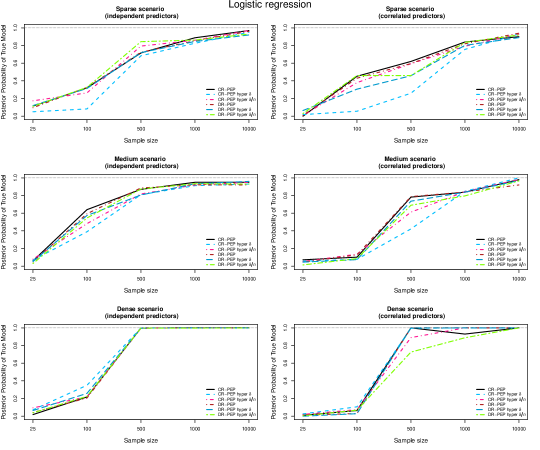
Figure 1: Posterior probabilities of the true model vs. sample size for the sparse, medium and dense logistic regression scenarios.

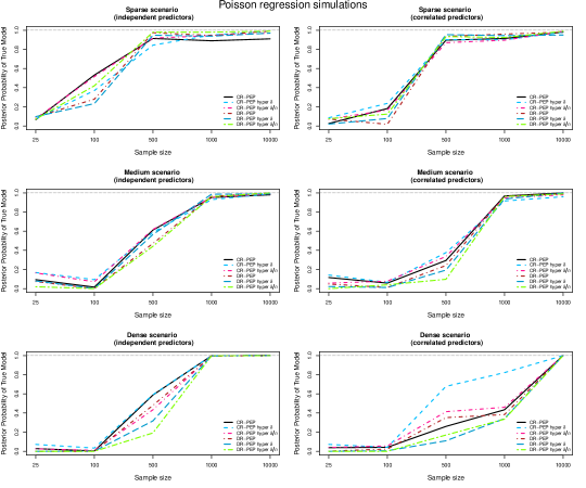
Figure 2: Posterior probabilities of the true model vs. sample size for the sparse, medium and dense Poisson regression scenarios.

7.3 Simulation study 2

In this illustration we consider a more sophisticated scenario with $p=10$ potential predictors ($1024$ models) and a more intriguing correlation structure. Similar to Nott and Kohn (2005), the first five covariates are generated from a standard normal distribution, while the remaining five covariates are generated from

$$X_{ij}=N(0.3X_{i1}+0.5X_{i2}+0.7X_{i3}+0.9X_{i4}+1.1X_{i5},1),$$

for $i=1,\dots,n$ and $j=6,\dots,10$. We assume that sample size $n$ is 200 and consider the three logistic regression data-generating models which are summarized in Table 7; the resulting odds ratios for the sparse and dense simulation models are approximately equal to 2 and 3, respectively. Each simulation is repeated 100 times.

In this example we use the beta-binomial prior (2.29) with a Beta(1,1) mixing distribution; see Scott and Berger (2010). The comparison that follows is based on the posterior inclusion probability of each covariate. Figures 3, 4 and 5 present boxplots of the posterior inclusion probabilities from the 100 simulated data sets for the null, sparse and dense simulation scenarios, respectively.

Scenario	Logistic  $(n=200)$
	$\beta_{0}$	$\beta_{1}$	$\beta_{2}$	$\beta_{3}$	$\beta_{4}$	$\beta_{5}$	$\beta_{6}$	$\beta_{7}$	$\beta_{8}$	$\beta_{9}$	$\beta_{10}$
null	0.1	0	0	0	0	0	0	0	0	0	0
sparse	0.1	0	0	-0.9	0	0	0	1.2	0	0	0.4
dense	0.1	0.6	0	-0.9	0	1	0.9	1.2	-1.2	-0.5	0

Table 7: Three logistic simulation scenarios for Simulation Study 2.

Under the null scenario, all priors, except the hyper-$g$ prior, exhibit strong shrinkage towards zero on the inclusion probabilities. Under the hyper-$g$ prior relatively large posterior inclusion probabilities with high variability across different samples are obtained. The hyper-$\delta$ CR-PEP prior also induces more variability, however, the resulting inclusion probabilities under this method are quite lower in comparison to those obtained under the hyper-$g$ prior.

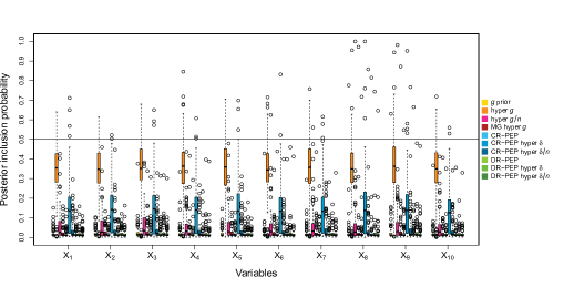
Figure 3: Posterior inclusion probabilities for Simulation Study 2 under the various priors from 100 repetitions of the null logistic simulation scenario.

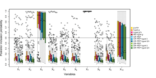
Figure 4: Posterior inclusion probabilities for Simulation Study 2 under the various priors from 100 repetitions of the sparse logistic simulation scenario where the true model is $X_{3}+X_{7}+X_{10}$.

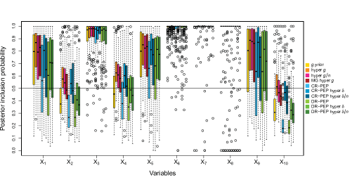
Figure 5: Posterior inclusion probabilities for Simulation Study 2 under the various priors from 100 repetitions of the dense logistic simulation scenario where the true model is $X_{1}+X_{3}+X_{5}+X_{6}+X_{7}+X_{8}+X_{9}$.

Under the sparse scenario (true model: $X_{1}+X_{7}+X_{10}$), there are no striking differences among all methods. All priors provide very strong support for the inclusion of $X_{7}$ and sufficient support for the inclusion of $X_{3}$, although the variability under PEP priors is larger for the latter variable. Moreover, all methods yield very wide posterior inclusion probability intervals for predictor $X_{10}$, implying high posterior uncertainty concerning the inclusion of this variable. For the non-important variables we observe that the fixed-$\delta$ CR-PEP and the DR-PEP priors yield the lowest posterior inclusion probabilities.

Finally, in the dense simulation scenario (Figure 5), where the true model is $X_{1}+X_{3}+X_{5}+X_{6}+X_{7}+X_{8}+X_{9}$, the fixed-$\delta$ PEP priors generally outperform other methods in terms of providing low posterior inclusion probabilities for the insignificant covariates $X_{2}$, $X_{4}$ and $X_{10}$. The $g$-prior and the hyper DR-PEP extensions yield similar posterior inclusion probabilities and generally perform well, however, they introduce some uncertainty concerning the inclusion of covariate $X_{4}$. The rest of the methods systematically support more complex models as they provide elevated support for the inclusion of variables $X_{2}$ and $X_{4}$.

7.4 A real life example

In our last example we consider the Pima Indians diabetes data set (Ripley, 1996), which has been analyzed in several studies (e.g. Holmes and Held, 2006; Sabanés Bové and Held, 2011). The data consist of $n=532$ complete records on diabetes presence (present=1, not present=0) according to the WHO criteria for signs of diabetes. The presence of diabetes is associated with $p=7$ potential covariates which are listed in Table 8.

For each method we used 41000 iterations of the GVS algorithm, discarding the first 1000 as burn-in period. We assigned a beta-binomial prior on model space (see Eq. 2.29) with both hyper-parameters equal to one. Table 9 shows the posterior inclusion probabilities of each covariate under the various methods. For comparison with the results presented in Sabanés Bové and Held (2011), we also include in Table 9 the resulting posterior inclusion probabilities from the Zellner and Siow (1980) inverse gamma (ZS-IG) prior, the hyper-$g/n$ with $a=4$, and a non-informative inverse gamma (NI-IG) hyper-$g$ prior with shape and scale equal to $10^{-3}$. As seen, the posterior inclusion probabilities that we obtain from the GVS algorithm are in agreement with the results presented in Sabanés Bové and Held (2011).

Covariate	Description
$X_{1}$	Number of pregnancies
$X_{2}$	Plasma glucose concentration (mg/dl)
$X_{3}$	Diastolic blood pressure (mm Hg)
$X_{4}$	Triceps skin fold thickness (mm)
$X_{5}$	Body mass index (kg/m2)
$X_{6}$	Diabetes pedigree function
$X_{7}$	Age

Table 8: Potential predictors in the Pima Indians diabetes data set.

Method	Predictor
	$X_{1}$	$X_{2}$	$X_{3}$	$X_{4}$	$X_{5}$	$X_{6}$	$X_{7}$
ZS-IG hyper-$g$	0.961	1.000	0.252	0.250	0.998	0.994	0.530
NI-IG hyper-$g$	0.967	1.000	0.349	0.341	0.998	0.996	0.622
$g$-prior ($g=n$)	0.952	1.000	0.136	0.139	0.998	0.992	0.382
hyper-$g$ ($a=3$)	0.970	1.000	0.397	0.379	0.998	0.996	0.669
hyper-$g/n$ ($a=3$)	0.966	1.000	0.304	0.300	0.998	0.995	0.579
hyper-$g/n$ $(a=4)$	0.965	1.000	0.307	0.299	0.997	0.995	0.582
MG hyper-$g$	0.958	1.000	0.262	0.259	0.998	0.994	0.548
CR-PEP	0.948	1.000	0.100	0.104	0.998	0.987	0.339
CR-PEP hyper-$\delta$	0.964	1.000	0.296	0.291	0.998	0.995	0.602
CR-PEP hyper-$\delta/n$	0.956	1.000	0.223	0.225	0.998	0.992	0.520
DR-PEP	0.948	1.000	0.102	0.104	0.997	0.988	0.324
DR-PEP hyper-$\delta$	0.954	1.000	0.174	0.173	0.997	0.991	0.442
DR-PEP hyper-$\delta/n$	0.951	1.000	0.125	0.120	0.998	0.987	0.346

Table 9: Posterior inclusion probabilities for the seven covariates of the Pima Indians data set.

For the covariates $X_{1},X_{2},X_{5}$ and $X_{6}$, which seem to be highly influential, the results in Table 9 show no significant differences among methods. On the contrary, the posterior inclusion probabilities for the “uncertain” covariates $X_{3},X_{4}$ and $X_{7}$ vary substantially; specifically, the inclusion probabilities from the fixed-$\delta$ CR/DR-PEP priors, the hyper-$\delta/n$ DR-PEP prior and the $g$-prior are considerably lower than the inclusion probabilities resulting from the rest of the methods. In terms of the shrinkage factors $g/(g+1)$ and $\delta/(\delta+1)$, results show that the shrinkage effect is stronger when $g$ or $\delta$ is fixed, which leads to a drastic reduction in the effects (and the inclusion probabilities) of low-influential covariates. On the other hand, the priors with random $g$ or $\delta$ clearly result in higher posterior inclusion probabilities. Among this category of priors, the hyper-$\delta/n$ DR-PEP is evidently the most parsimonious, as it yields posterior inclusion probabilities which are actually quite close to those obtained from fixed $\delta$ PEP priors.

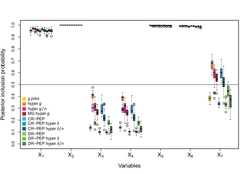
Figure 6: Boxplots of batched estimates of the posterior inclusion probabilities for the seven predictors in the Pima Indians data set based on 40 batches of size 1000.

The uncertainty of the estimated posterior inclusion probabilities, for the standard methods considered in the previous examples, is depicted in Figure 6, where we present the corresponding boxplots produced by splitting the posterior samples into 40 batches of size 1000. As seen in Figure 6, stochasticity in $g$ and $\delta$ mainly affects the posterior inclusion probabilities of the “uncertain” covariates $X_{3},X_{4}$ and $X_{7}$. For these variables the extra prior uncertainty induces higher posterior variability, as expected, and consequently larger Monte Carlo errors. Apart from this, we generally observe the same patterns of evidence leading to the conclusions discussed in Sections 7.2 and 7.3.

Figure 7 depicts the convergence and the estimated posterior distribution of the shrinkage parameter $\delta/(1+\delta)$ under the four PEP hyper-prior approaches. The posterior histograms are indicative of the behavior of the shrinkage parameter. Comparison between the hyper-$\delta$ (Figure 7a) and the hyper-$\delta/n$ (Figure 7b) approaches shows that the posterior distribution of the shrinkage parameter under the latter priors is more concentrated to values close to one, thus, resulting to a stronger shrinkage effect. Also, the histograms in Figures 7a and 7b indicate that the posterior distributions of the shrinkage parameter under DR-PEP are more concentrated to one in comparison to the corresponding posteriors under CR-PEP. Note that the shrinkage under the fixed-$\delta$ approaches is constant, equal to 0.998, which leads to considerably lower posterior inclusion probabilities as seen in Table 9 and Figure 6.

(a) Hyper-$\delta$ Priors	(b) Hyper-$\delta/n$ Priors

Figure 7: Ergodic mean plots, time-series plots and histograms of the shrinkage factor $\delta/(1+\delta)$ for the hyper-$\delta$ and hyper-$\delta/n$ PEP priors based on 40000 draws.

We conclude this example by examining the out-of-sample predictive accuracy of the various prior setups. We randomly split the data set in half in order to create a training sample and a test sample and identified the corresponding MAP and the median probability models, under all methods, from the training data set. Then, based on posterior samples from the predictive distribution we calculated the averages of false positive and false negative percentages for the test data set; the results are reported in Table 10. Overall, we cannot say that there is dominant method in terms of predictive accuracy as the predictions are more or less the same across the prior setups. We may note however that the most complex MAP model arises from the hyper-$g$ prior which also results in the highest false negative prediction rates. Also, the unit-information $g$-prior, the CR-PEP prior with fixed $\delta$, and the DR-PEP priors lead to the most parsimonious median probability model. This model is comparable in terms of predictive performance with the model that further includes $X_{7}$, which is indicated as the median probability model by the rest of the methods.

		False	False		False	False
		Neg.	Pos.		Neg.	Pos.
Method	MAP	(%)	(%)	MPM	(%)	(%)
$g$-prior ($g=n$)	${\cal M}_{A}$	10.8	16.5	${\cal M}_{A}$	10.8	16.5
hyper-$g$ ($a=3$)	${\cal M}_{A}+X_{3}+X_{4}+X_{7}$	11.4	16.9	${\cal M}_{A}+X_{7}$	11.1	16.8
hyper-$g/n$ ($a=3$)	${\cal M}_{A}$	11.0	16.6	${\cal M}_{A}+X_{7}$	11.0	16.6
MG hyper-$g$	${\cal M}_{A}$	10.9	16.6	${\cal M}_{A}+X_{7}$	10.9	16.6
CR-PEP	${\cal M}_{A}$	10.9	16.9	${\cal M}_{A}$	10.9	16.9
CR-PEP hyper-$\delta$	${\cal M}_{A}$	10.9	17.0	${\cal M}_{A}+X_{7}$	11.3	16.4
CR-PEP hyper-$\delta/n$	${\cal M}_{A}$	10.8	17.0	${\cal M}_{A}+X_{7}$	11.0	16.6
DR-PEP	${\cal M}_{A}$	10.9	16.8	${\cal M}_{A}$	10.9	16.8
DR-PEP hyper-$\delta$	${\cal M}_{A}$	10.9	16.9	${\cal M}_{A}$	10.9	16.9
DR-PEP hyper-$\delta/n$	${\cal M}_{A}$	10.9	16.8	${\cal M}_{A}$	10.9	16.8
${\cal M}_{A}:X_{1}+X_{2}+X_{5}+X_{6}$

Table 10: Percentages of false negative and false positive detections for the Pima Indian data set under the MAP model and median probability model (MPM) for the various priors.

8 Discussion

In this paper we presented an objective, automatic and compatible across competing models Bayesian procedure with applications to the variable selection problem in GLMs. Specifically we extended the PEP prior formulation through the use of unnormalized power likelihoods and defined two new PEP priors, called CR-PEP and DR-PEP, which differentiate with respect to the definition of the prior predictive distribution of the reference model. Under the new definitions, the applicability of the PEP methodology is significantly enhanced. Although we focused on variable selection for GLMs, the CR/DR-PEP priors proposed here may in principle be used for any general model setting. At the same time the new approaches retain the desired features of the original PEP prior formulation; specifically, i) they resolve the problem of selecting and averaging across minimal imaginary samples, thus, also allowing for large-sample approximations, and ii) they are minimally informative as they scale down the effect of the imaginary data on the posterior distribution. We further studied the assignment of hyper-prior distributions to the power parameter $\delta$ that controls the contribution of the imaginary data. Following the hyper-$g$ and $g/n$ priors proposed in Liang et al. (2008), we effectively introduced the hyper-$\delta$ and $\delta/n$ analogues.

With respect to the criteria of Bayarri et al. (2012), we provided analytical proofs for the null and dimensional predictive matching criteria for all PEP priors under consideration. With respect to model selection consistency, analytical proofs for the normal linear model are provided in Fouskakis et al. (2016); here, we illustrated through simulations that this criterion also seems to be valid within the PEP priors framework for specific GLMs scenarios.

The empirical results presented in this paper suggest that the proposed PEP priors outperform mixtures of $g$-priors in terms of introducing larger shrinkage to the inclusion probabilities of non-influential or partially influential predictors, thus, leading to more parsimonious solutions with comparable predictive accuracy. When comparing PEP priors with fixed $\delta=n$ and random $\delta$ the results indicate that the former approach induces more stringent control in the inclusion of predictors. Therefore, fixed PEP priors support simpler models which is a desirable feature when the number of covariates is large. Concerning the choice between the CR and the DR prior setups, we conclude in favour to the use of the latter since it is rather robust with respect to the fixed vs. random specification of $\delta$.

In future research we plan to extend the PEP methodology to high-dimensional problems, including the small $n$–large $p$ case, by incorporating shrinkage priors (e.g. ridge and LASSO procedures) into the PEP design. Another promising alternative is to embody the expectation-maximization variable selection approach of Ročková and George (2014) within the PEP prior.

Appendix

Appendix A Proofs of Predictive Matching

A.1 Proof of Proposition 5.1.

Assuming known and common across all models $\phi_{\boldsymbol{\gamma}}=\phi$, then, for samples of size $n=1$ (and, therefore we have also $\delta=n^{*}=1$), both CR-PEP and DR-PEP priors coincide. Moreover, assuming that we have observed the response $y$ with covariate values ${\boldsymbol{x}}=(x_{1},\dots,x_{p})^{T}$ then we need to generate an imaginary data-point $y^{*}$ under the same set of covariates. Moreover, the linear predictor for any model ${\boldsymbol{\gamma}}$ is now given by

$$\eta_{\boldsymbol{\gamma}}=\beta_{0,{\boldsymbol{\gamma}}}+{\boldsymbol{x}}_{\boldsymbol{\gamma}}^{T}{\boldsymbol{\beta}}_{\setminus 0,{\boldsymbol{\gamma}}}=\beta_{0,{\boldsymbol{\gamma}}}+\sum_{j=1}^{p}\gamma_{j}x_{j}\beta_{j},$$ (A.1)

where ${\boldsymbol{x}}_{\boldsymbol{\gamma}}$ is the sub-vector of ${\boldsymbol{x}}$ with elements corresponding to covariates included in model $M_{\boldsymbol{\gamma}}$.

Under this formulation and (5.1), the prior predictive density for model $M_{0}$ under the baseline prior $\pi_{0}^{N}(\beta_{0})$ is given by

$$m_{0}^{\mathrm{N}}(y^{*}|\delta=1) = \int\exp\left(\frac{y^{*}\vartheta(\beta_{0})-b\big{(}\vartheta(\beta_{0})\big{)}}{a(\phi)}+c(y^{*},\phi)\right)\psi(\beta_{0})d\beta_{0}.$$

By setting $\eta=\beta_{0}$ under model $M_{0}$, we obtain

$$m_{0}^{\mathrm{N}}(y^{*}|\delta=1) = e^{c(y^{*},\phi)}{\cal D}(y^{*},1,1)$$

$$\mbox{where~{}}{\cal D}(y,\omega,\delta)=\int\exp\left(\frac{y^{*}\vartheta(\eta)-\omega b\big{(}\vartheta(\eta)\big{)}}{\delta a(\phi)}\right)\psi(\eta)d\eta.$$

For model $M_{\boldsymbol{\gamma}}$, the prior predictive density under the baseline prior $\pi_{\boldsymbol{\gamma}}^{N}(\boldsymbol{\beta}_{\boldsymbol{\gamma}})$ is given by

$$m_{\boldsymbol{\gamma}}^{\mathrm{N}}(y^{*}|\delta=1) = \int\exp\left(\frac{y^{*}\vartheta(\eta_{\boldsymbol{\gamma}})-b\big{(}\vartheta(\eta_{\boldsymbol{\gamma}})\big{)}}{a(\phi)}+c(y^{*},\phi)\right)\psi(\eta_{\gamma})\Psi_{\boldsymbol{\gamma}}({\boldsymbol{\beta}}_{\setminus 0,{\boldsymbol{\gamma}}})d\boldsymbol{\beta}_{\boldsymbol{\gamma}}.\hskip 20.00003pt$$ (A.3)

By setting $\eta=\beta_{0,{\boldsymbol{\gamma}}}+\sum_{j=1}^{p}\gamma_{j}x_{j}\beta_{j}=\eta_{\boldsymbol{\gamma}}$ (see Eq. A.1) and ${\boldsymbol{b}}={\boldsymbol{\beta}}_{\setminus 0,{\boldsymbol{\gamma}}}$, then from (A.3) we obtain

$$m_{\boldsymbol{\gamma}}^{\mathrm{N}}(y^{*}|\delta=1) = e^{c(y^{*},\phi)}\int\left\{\int\exp\left(\frac{y^{*}\vartheta(\eta)-b\big{(}\vartheta(\eta)\big{)}}{a(\phi)}\right)\psi(\eta)d\eta\right\}\Psi_{\boldsymbol{\gamma}}({\boldsymbol{b}})d{\boldsymbol{b}}$$

$$= e^{c(y^{*},\phi)}{\cal D}(y^{*},1,1){\cal A}_{\boldsymbol{\gamma}}=m_{0}^{N}(y^{*}|\delta=1){\cal A}_{\boldsymbol{\gamma}},$$

where ${\cal A}_{\boldsymbol{\gamma}}=\int\Psi_{\boldsymbol{\gamma}}({\boldsymbol{b}})d{\boldsymbol{b}}$.

The marginal likelihood of $M_{0}$ under the PEP prior is given by

$$m_{0}^{\mathrm{PEP}}(y|\delta=1)=m_{0}^{N}(y|\delta=1),$$

while for model $M_{\boldsymbol{\gamma}}$ is given by

$$m_{\boldsymbol{\gamma}}^{\mathrm{PEP}}(y|\delta=1) = \int\frac{m_{0}^{\mathrm{N}}(y^{*}|\delta=1)}{m_{{\boldsymbol{\gamma}}}^{\mathrm{N}}(y^{*}|\delta=1)}\left\{\int{f_{{\boldsymbol{\gamma}}}(y|\boldsymbol{\beta}_{\boldsymbol{\gamma}})f_{{\boldsymbol{\gamma}}}(y^{*}|\boldsymbol{\beta}_{\boldsymbol{\gamma}},\delta=1)\pi_{{\boldsymbol{\gamma}}}^{\mathrm{N}}(\boldsymbol{\beta}_{\boldsymbol{\gamma}})}\mathrm{d}\boldsymbol{\beta}_{\boldsymbol{\gamma}}\right\}\mathrm{d}y^{*}$$

$$= \int{\cal A}^{-1}_{\boldsymbol{\gamma}}\left\{\int{f_{{\boldsymbol{\gamma}}}(y|\boldsymbol{\beta}_{\boldsymbol{\gamma}})f_{{\boldsymbol{\gamma}}}(y^{*}|\boldsymbol{\beta}_{\boldsymbol{\gamma}},\delta=1)\pi_{{\boldsymbol{\gamma}}}^{\mathrm{N}}(\boldsymbol{\beta}_{\boldsymbol{\gamma}})}\mathrm{d}\boldsymbol{\beta}_{\boldsymbol{\gamma}}\right\}\mathrm{d}y^{*}$$

$$= \int{\cal A}^{-1}_{\boldsymbol{\gamma}}\left\{f_{{\boldsymbol{\gamma}}}(y|\boldsymbol{\beta}_{\boldsymbol{\gamma}})\left[\int f_{{\boldsymbol{\gamma}}}(y^{*}|\boldsymbol{\beta}_{\boldsymbol{\gamma}},\delta=1)\mathrm{d}y^{*}\right]\pi_{{\boldsymbol{\gamma}}}^{\mathrm{N}}(\boldsymbol{\beta}_{\boldsymbol{\gamma}})\right\}\mathrm{d}\boldsymbol{\beta}_{\boldsymbol{\gamma}}$$

$$= {\cal A}^{-1}_{\boldsymbol{\gamma}}\int f_{{\boldsymbol{\gamma}}}(y|\boldsymbol{\beta}_{\boldsymbol{\gamma}})\pi_{{\boldsymbol{\gamma}}}^{\mathrm{N}}(\boldsymbol{\beta}_{\boldsymbol{\gamma}})\mathrm{d}\boldsymbol{\beta}_{\boldsymbol{\gamma}}={\cal A}^{-1}_{\boldsymbol{\gamma}}m_{\boldsymbol{\gamma}}^{N}(y|\delta=1)$$

$$= {\cal A}^{-1}_{\boldsymbol{\gamma}}m_{0}^{N}(y|\delta=1){\cal A}_{\boldsymbol{\gamma}}=m_{0}^{N}(y|\delta=1)$$

and hence, for known $\phi$, this concludes the proof.

If $\phi$ is stochastic and common across models, then the two marginal likelihoods, obtained by integrating out $\phi$ over the common prior $\pi^{N}_{0}(\phi)=\pi^{N}_{\boldsymbol{\gamma}}(\phi)$ for all models $M_{\boldsymbol{\gamma}}$, still coincide.

A.2 Proof of Proposition 5.2.

Following similar arguments as in Section A.1 we have that

$$m_{0}^{\mathrm{N}}(y^{*}|\delta) = e^{c(y^{*},\phi)/\delta}{\cal D}(y^{*},1,\delta)$$

$$m_{\boldsymbol{\gamma}}^{\mathrm{N}}(y^{*}|\delta) = e^{c(y^{*},\phi)/\delta}{\cal D}(y^{*},1,\delta){\cal A}_{\boldsymbol{\gamma}}=m_{0}^{N}(y^{*}|\delta){\cal A}_{\boldsymbol{\gamma}}.$$ (A.4)

The final marginal likelihood of $M_{\boldsymbol{\gamma}}$ under the DR-PEP prior, conditional on $\delta$, is given by

$$m_{\boldsymbol{\gamma}}^{\mathrm{DR-PEP}}(y|\delta) = {\cal C}_{0}^{-1}\int\frac{m_{0}^{\mathrm{N}}(y^{*}|\delta)}{m_{{\boldsymbol{\gamma}}}^{\mathrm{N}}(y^{*}|\delta)}\left\{\int{f_{{\boldsymbol{\gamma}}}(y|\boldsymbol{\beta}_{\boldsymbol{\gamma}})f_{{\boldsymbol{\gamma}}}(y^{*}|\boldsymbol{\beta}_{\boldsymbol{\gamma}},\delta)\pi_{{\boldsymbol{\gamma}}}^{\mathrm{N}}(\boldsymbol{\beta}_{\boldsymbol{\gamma}})}\mathrm{d}\boldsymbol{\beta}_{\boldsymbol{\gamma}}\right\}\mathrm{d}y^{*}$$

$$= {\cal C}_{0}^{-1}\int{\cal A}^{-1}_{\boldsymbol{\gamma}}\left\{\int{f_{{\boldsymbol{\gamma}}}(y|\boldsymbol{\beta}_{\boldsymbol{\gamma}})f_{{\boldsymbol{\gamma}}}(y^{*}|\boldsymbol{\beta}_{\boldsymbol{\gamma}},\delta)\pi_{{\boldsymbol{\gamma}}}^{\mathrm{N}}(\boldsymbol{\beta}_{\boldsymbol{\gamma}})}\mathrm{d}\boldsymbol{\beta}_{\boldsymbol{\gamma}}\right\}\mathrm{d}y^{*}$$

$$= {\cal C}_{0}^{-1}{\cal A}^{-1}_{\boldsymbol{\gamma}}\int\int\exp\left(\frac{y\vartheta(\eta_{\boldsymbol{\gamma}})-b\big{(}\vartheta(\eta_{\boldsymbol{\gamma}})\big{)}}{a(\phi)}+c(y,\phi)\right)$$

$$\hskip 32.00002pt\times\exp\left(\frac{y^{*}\vartheta(\eta_{\boldsymbol{\gamma}})-b\big{(}\vartheta(\eta_{\boldsymbol{\gamma}})\big{)}}{\delta a(\phi)}+\frac{c(y^{*},\phi)}{\delta}\right)\pi_{{\boldsymbol{\gamma}}}^{\mathrm{N}}(\boldsymbol{\beta}_{\boldsymbol{\gamma}})\mathrm{d}\boldsymbol{\beta}_{\boldsymbol{\gamma}}\mathrm{d}y^{*}.$$

By using (5.1) and setting $\eta=\beta_{0,{\boldsymbol{\gamma}}}+\sum_{j=1}^{p}\gamma_{j}x_{j}\beta_{j}=\eta_{\boldsymbol{\gamma}}$ (see Eq. A.1) and ${\boldsymbol{b}}={\boldsymbol{\beta}}_{\setminus 0,{\boldsymbol{\gamma}}}$, we obtain

$$m_{\boldsymbol{\gamma}}^{\mathrm{DR-PEP}}(y|\delta)={\cal C}_{0}^{-1}{\cal A}^{-1}_{\boldsymbol{\gamma}}\times$$

$$\times\int e^{c(y,\phi)+c(y^{*},\phi)/\delta}\left\{\int\exp\left(\frac{(\delta y+y^{*})\vartheta(\eta)-(\delta+1)b\big{(}\vartheta(\eta)\big{)}}{\delta a(\phi)}\right)\psi(\eta)\mathrm{d}\eta\int\Psi_{\boldsymbol{\gamma}}({\boldsymbol{b}})\mathrm{d}{\boldsymbol{b}}\right\}\mathrm{d}y^{*}.$$

$$= {\cal C}_{0}^{-1}e^{c(y,\phi)}\int e^{c(y^{*},\phi)/\delta}{\cal D}(\delta y+y^{*},\delta+1,\delta)\mathrm{d}y^{*}$$

which does not depend on the original model formulation $M_{\boldsymbol{\gamma}}$. Indeed, following similar logic we can prove that

$$m_{0}^{\mathrm{DR-PEP}}(y|\delta)={\cal C}_{0}^{-1}e^{c(y,\phi)}\int e^{c(y^{*},\phi)/\delta}{\cal D}(\delta y+y^{*},\delta+1,\delta)\mathrm{d}y^{*},$$

and hence, for known $\phi$, it is obvious that after integrating out $\delta$ over the hyper-prior $\pi(\delta)$, $m_{\boldsymbol{\gamma}}^{\mathrm{DR-PEP}}(y)=m_{0}^{\mathrm{DR-PEP}}(y)$ and this concludes the proof.

If $\phi$ is stochastic and common across models, then the two marginal likelihoods, obtained by integrating out $\phi$ over the common prior $\pi^{N}_{0}(\phi)=\pi^{N}_{\boldsymbol{\gamma}}(\phi)$ for all models $M_{\boldsymbol{\gamma}}$, still coincide.

A.3 Proof of Proposition 5.3.

For the CR-PEP prior, conditional on $\delta$, using (5.1), (A.1) and (A.4) and following similar steps as in Appendix A.1 we have that

$$m_{\boldsymbol{\gamma}}^{\mathrm{CR-PEP}}(y|\delta) = \int\frac{m_{0}^{\mathrm{N}}(y^{*}|\delta=1)}{m_{{\boldsymbol{\gamma}}}^{\mathrm{N}}(y^{*}|\delta)}\left\{\int{f_{{\boldsymbol{\gamma}}}(y|\boldsymbol{\beta}_{\boldsymbol{\gamma}})f_{{\boldsymbol{\gamma}}}(y^{*}|\boldsymbol{\beta}_{\boldsymbol{\gamma}},\delta)\pi_{{\boldsymbol{\gamma}}}^{\mathrm{N}}(\boldsymbol{\beta}_{\boldsymbol{\gamma}})}\mathrm{d}\boldsymbol{\beta}_{\boldsymbol{\gamma}}\right\}\mathrm{d}y^{*}$$

$$= \int{\cal A}^{-1}_{\boldsymbol{\gamma}}e^{\frac{\delta-1}{\delta}c(y^{*},\phi)}\frac{{\cal D}(y^{*},1,1)}{{\cal D}(y^{*},1,\delta)}\left\{\int{f_{{\boldsymbol{\gamma}}}(y|\boldsymbol{\beta}_{\boldsymbol{\gamma}})f_{{\boldsymbol{\gamma}}}(y^{*}|\boldsymbol{\beta}_{\boldsymbol{\gamma}},\delta)\pi_{{\boldsymbol{\gamma}}}^{\mathrm{N}}(\boldsymbol{\beta}_{\boldsymbol{\gamma}})}\mathrm{d}\boldsymbol{\beta}_{\boldsymbol{\gamma}}\right\}\mathrm{d}y^{*}$$

$$= e^{c(y,\phi)}\int e^{c(y^{*},\phi)}\frac{{\cal D}(y^{*},1,1)}{{\cal D}(y^{*},1,\delta)}{\cal D}(\delta y+y^{*},\delta+1,\delta)\mathrm{d}y^{*}$$

which (again) does not depend on the original model formulation $M_{\boldsymbol{\gamma}}$. Hence, for known $\phi$, it is obvious that after integrating out $\delta$ over the hyper-prior $\pi(\delta)$, $m_{\boldsymbol{\gamma}}^{\mathrm{CR-PEP}}(y)=m_{0}^{\mathrm{CR-PEP}}(y)$ and this concludes the proof.

If $\phi$ is stochastic and common across models, then the two marginal likelihoods, obtained by integrating out $\phi$ over the common prior $\pi^{N}_{0}(\phi)=\pi^{N}_{\boldsymbol{\gamma}}(\phi)$ for all models $M_{\boldsymbol{\gamma}}$, still coincide.

A.4 Proof of Proposition 5.4.

Let us assume known and common across models $\phi_{\boldsymbol{\gamma}}=\phi$ and samples of size $n=p_{\boldsymbol{\gamma}}+1=\sum_{j=1}^{p}+1$. Then the linear predictor is given by ${\boldsymbol{\eta}}_{\boldsymbol{\gamma}}=\mathrm{X}_{\boldsymbol{\gamma}}\boldsymbol{\beta}_{\boldsymbol{\gamma}}$ where $\mathrm{X}_{\boldsymbol{\gamma}}$ is a matrix of dimension $(p_{\boldsymbol{\gamma}}+1)\times(p_{\boldsymbol{\gamma}}+1)$. By considering $n^{*}=n=1+p_{\boldsymbol{\gamma}}$ and further assuming that is invertible, then the prior predictive density for model $M_{0}$ under the baseline prior $\pi_{0}^{N}(\beta_{0})$ is given by

$$m_{0}^{\mathrm{N}}(\mathbf{y}^{*}|\delta) = \int\exp\left(\frac{n^{*}\overline{y}^{*}\vartheta(\beta_{0})-n^{*}b\big{(}\vartheta(\beta_{0})\big{)}}{\delta a(\phi)}+\sum_{i=1}^{n^{*}}\frac{c(y_{i}^{*},\phi)}{\delta}\right)\psi(\beta_{0})d\beta_{0}$$

By setting $\eta=\beta_{0}$, we obtain

$$m_{0}^{\mathrm{N}}(\mathbf{y}^{*}|\delta) = \exp\left(\sum_{i=1}^{n^{*}}\frac{c(y_{i}^{*},\phi)}{\delta}\right){\cal D}(n^{*}\overline{y}^{*},n^{*},\delta).$$

For model $M_{\boldsymbol{\gamma}}$, the prior predictive density under the baseline prior $\pi_{\boldsymbol{\gamma}}^{N}(\boldsymbol{\beta}_{\boldsymbol{\gamma}})$ is given by

$$m_{\boldsymbol{\gamma}}^{\mathrm{N}}(\mathbf{y}^{*}|\delta) = \int\exp\left(\frac{\sum_{i=1}^{n^{*}}y_{i}^{*}\vartheta(\eta_{{\boldsymbol{\gamma}}(i)})-\sum_{i=1}^{n^{*}}b\big{(}\vartheta(\eta_{{\boldsymbol{\gamma}}(i)})\big{)}}{\delta a(\phi)}+\sum_{i=1}^{n^{*}}\frac{c(y_{i}^{*},\phi)}{\delta}\right)\psi({\boldsymbol{\eta}}_{\gamma})d\boldsymbol{\beta}_{\boldsymbol{\gamma}}~{}.$$

By setting ${\boldsymbol{\eta}}=\mathrm{X}_{\boldsymbol{\gamma}}\boldsymbol{\beta}_{\boldsymbol{\gamma}}={\boldsymbol{\eta}}_{\gamma}$, we obtain

$$m_{\boldsymbol{\gamma}}^{\mathrm{N}}(\mathbf{y}^{*}|\delta) = \exp\left(\sum_{i=1}^{n^{*}}\frac{c(y_{i}^{*},\phi)}{\delta}\right)\int\exp\left(\frac{\sum_{i=1}^{n^{*}}y_{i}^{*}\vartheta(\eta_{i})-\sum_{i=1}^{n^{*}}b\big{(}\vartheta(\eta_{i})\big{)}}{\delta a(\phi)}\right)\psi({\boldsymbol{\eta}})|\mathrm{X}_{\boldsymbol{\gamma}}^{-1}|d{\boldsymbol{\eta}}$$

$$= \exp\left(\sum_{i=1}^{n^{*}}\frac{c(y_{i}^{*},\phi)}{\delta}\right)|\mathrm{X}_{\boldsymbol{\gamma}}^{-1}|{\cal E}(\mathbf{y}^{*},1,\delta)$$

$$\mbox{where~{}}{\cal E}(\mathbf{y}^{*},\omega,\delta)=\int\exp\left(\frac{\sum_{i=1}^{n^{*}}y_{i}^{*}\vartheta(\eta_{i})-\omega\sum_{i=1}^{n^{*}}b\big{(}\vartheta(\eta_{i})\big{)}}{\delta a(\phi)}\right)\psi({\boldsymbol{\eta}})d{\boldsymbol{\eta}};$$

note that ${\cal E}(y^{*},\omega,\delta)={\cal D}(y^{*},\omega,\delta)$ for $n^{*}=1$.

The marginal likelihood of $M_{0}$ under the DR-PEP prior, conditional on $\delta$, is given by $m_{0}^{\mathrm{DR-PEP}}(\mathbf{y}|\delta)=m_{0}^{N}(\mathbf{y}|\delta)$ while for model $M_{\boldsymbol{\gamma}}$ is given by

$$m_{\boldsymbol{\gamma}}^{\mathrm{DR-PEP}}(\mathbf{y}|\delta) = {\cal C}_{0}^{-1}\int|\mathrm{X}_{\boldsymbol{\gamma}}|\frac{{\cal D}(n^{*}\overline{y}^{*},n^{*},\delta)}{{\cal E}(\mathbf{y}^{*},1,\delta)}\left\{\int{f_{{\boldsymbol{\gamma}}}(y|\boldsymbol{\beta}_{\boldsymbol{\gamma}})f_{{\boldsymbol{\gamma}}}(y^{*}|\boldsymbol{\beta}_{\boldsymbol{\gamma}},\delta)\pi_{{\boldsymbol{\gamma}}}^{\mathrm{N}}(\boldsymbol{\beta}_{\boldsymbol{\gamma}})}\mathrm{d}\boldsymbol{\beta}_{\boldsymbol{\gamma}}\right\}\mathrm{d}\mathbf{y}^{*}$$

$$= {\cal C}_{0}^{-1}|\mathrm{X}_{\boldsymbol{\gamma}}|\int\frac{{\cal D}(n^{*}\overline{y}^{*},n^{*},\delta)}{{\cal E}(\mathbf{y}^{*},1,\delta)}\left\{\int{f_{{\boldsymbol{\gamma}}}(y|\boldsymbol{\beta}_{\boldsymbol{\gamma}})f_{{\boldsymbol{\gamma}}}(y^{*}|\boldsymbol{\beta}_{\boldsymbol{\gamma}},\delta)\pi_{{\boldsymbol{\gamma}}}^{\mathrm{N}}(\boldsymbol{\beta}_{\boldsymbol{\gamma}})}\mathrm{d}\boldsymbol{\beta}_{\boldsymbol{\gamma}}\right\}\mathrm{d}\mathbf{y}^{*}$$

$$= {\cal C}_{0}^{-1}|\mathrm{X}_{\boldsymbol{\gamma}}|\int\frac{{\cal D}(n^{*}\overline{y}^{*},n^{*},\delta)}{{\cal E}(\mathbf{y}^{*},1,\delta)}\exp\left(\sum_{i=1}^{n^{*}}c(y_{i},\phi)+\sum_{i=1}^{n^{*}}\frac{c(y_{i}^{*},\phi)}{\delta}\right)$$

$$\hskip 150.00023pt\times|\mathrm{X}_{\boldsymbol{\gamma}}|^{-1}{\cal E}(\delta\mathbf{y}+\mathbf{y}^{*},\delta+1,\delta)\mathrm{d}\mathbf{y}^{*}$$

$$= {\cal C}_{0}^{-1}\int\prod_{i=1}^{n^{*}}e^{c(y_{i},\phi)+\frac{c(y_{i}^{*},\phi)}{\delta}}{\cal D}(n^{*}\overline{y}^{*},n^{*},\delta)\frac{{\cal E}(\delta\mathbf{y}+\mathbf{y}^{*},\delta+1,\delta)}{{\cal E}(\mathbf{y}^{*},1,\delta)}\mathrm{d}\mathbf{y}^{*}$$

which coincides for any model of the same dimension with training samples of the same size. Hence, for known $\phi$, this concludes the proof for the (fixed $\delta$) DR-PEP prior. It is obvious that for random $\delta$ integrating out the above marginal likelihoods over any hyper-prior $\pi(\delta)$ will result to $m_{\boldsymbol{\gamma}}^{\mathrm{DR-PEP}}(\mathbf{y})=m_{0}^{\mathrm{DR-PEP}}(\mathbf{y})$ and this concludes the proof for hyper-$\delta$ DR-PEP.

Finally if $\phi$ is stochastic and common across models, then the two marginal likelihoods (under fixed or random $\delta$), obtained by integrating out $\phi$ over the common prior $\pi^{N}_{0}(\phi)=\pi^{N}_{\boldsymbol{\gamma}}(\phi)$ for all models $M_{\boldsymbol{\gamma}}$, still coincide.

Appendix B The PEP-GVS algorithm

B.1 Implementation details

Concerning the binary inclusion indicators $\gamma_{j}$, the conditional posterior distribution $\pi\big{(}\gamma_{j}\big{|}\boldsymbol{\beta},{\boldsymbol{\gamma}}_{\setminus j},\mathbf{y}^{*},\mathbf{y},\delta\big{)}$ is a Bernoulli distribution with success probability $O_{j}/(1+O_{j})$ and

$$O_{j} = \frac{f_{{\boldsymbol{\gamma}}_{j_{1}}}\big{(}\mathbf{y}|\boldsymbol{\beta}_{{\boldsymbol{\gamma}}_{j_{1}}}\big{)}}{f_{{\boldsymbol{\gamma}}_{j_{0}}}\big{(}\mathbf{y}|\boldsymbol{\beta}_{{\boldsymbol{\gamma}}_{j_{0}}}\big{)}}\left[\frac{f_{{\boldsymbol{\gamma}}_{j_{1}}}(\mathbf{y}^{*}|\boldsymbol{\beta}_{{\boldsymbol{\gamma}}_{j_{1}}})}{f_{{\boldsymbol{\gamma}}_{j_{0}}}(\mathbf{y}^{*}|\boldsymbol{\beta}_{{\boldsymbol{\gamma}}_{j_{0}}})}\right]^{1/\delta}\frac{\pi^{\mathrm{N}}_{{\boldsymbol{\gamma}}_{j_{1}}}(\boldsymbol{\beta})}{\pi^{\mathrm{N}}_{{\boldsymbol{\gamma}}_{j_{0}}}(\boldsymbol{\beta})}\frac{{m}^{\mathrm{N}}_{{\boldsymbol{\gamma}}_{j_{0}}}(\mathbf{y}^{*}|\delta)}{{m}^{\mathrm{N}}_{{\boldsymbol{\gamma}}_{j_{1}}}(\mathbf{y}^{*}|\delta)}\frac{\pi({\boldsymbol{\gamma}}_{j_{1}})}{\pi({\boldsymbol{\gamma}}_{j_{0}})},$$ (B.1)

where ${\boldsymbol{\gamma}}_{j_{1}}=(\gamma_{j}=1,{\boldsymbol{\gamma}}_{\setminus j})$, ${\boldsymbol{\gamma}}_{j_{0}}=(\gamma_{j}=0,{\boldsymbol{\gamma}}_{\setminus j})$ and $\pi^{\mathrm{N}}_{\boldsymbol{\gamma}}(\boldsymbol{\beta})=\pi^{\mathrm{N}}_{\boldsymbol{\gamma}}(\boldsymbol{\beta}_{\boldsymbol{\gamma}})\pi^{\mathrm{N}}_{\boldsymbol{\gamma}}(\boldsymbol{\beta}_{\setminus{\boldsymbol{\gamma}}})$ for ${\boldsymbol{\gamma}}\in\{{\boldsymbol{\gamma}}_{j_{1}},{\boldsymbol{\gamma}}_{j_{0}}\}$. All of the quantities involved in (B.1) are available in closed form expressions except of the marginal likelihood $m_{\boldsymbol{\gamma}}^{\mathrm{N}}(\mathbf{y}^{*}|\delta)$. The latter is estimated through the following Laplace approximation

$$\widehat{m}_{{\boldsymbol{\gamma}}}^{\mathrm{N}}(\mathbf{y}^{*}|\delta)=(2\pi\delta)^{d_{{\boldsymbol{\gamma}}}/2}|\mathbf{X}_{{\boldsymbol{\gamma}}}^{T}\mathbf{W}_{{\boldsymbol{\gamma}}}(\widehat{\boldsymbol{\beta}}{}_{\boldsymbol{\gamma}}^{*})\mathbf{X}_{{\boldsymbol{\gamma}}}|^{-1/2}f_{\boldsymbol{\gamma}}\big{(}\mathbf{y}^{*}\big{|}\widehat{\boldsymbol{\beta}}{}_{\boldsymbol{\gamma}}^{*}\big{)}^{1/\delta}\pi^{\mathrm{N}}_{\boldsymbol{\gamma}}\big{(}\widehat{\boldsymbol{\beta}}{}_{\boldsymbol{\gamma}}^{*}\big{)},$$ (B.2)

where $\widehat{\boldsymbol{\beta}}{}_{\boldsymbol{\gamma}}^{*}$ is the MLE for data $\mathbf{y}^{*}$ given the configuration of ${\boldsymbol{\gamma}}$ and $\delta\Big{[}\mathbf{X}_{{\boldsymbol{\gamma}}}^{T}\mathbf{W}_{{\boldsymbol{\gamma}}}(\widehat{\boldsymbol{\beta}}{}_{\boldsymbol{\gamma}}^{*})\mathbf{X}_{{\boldsymbol{\gamma}}}\Big{]}^{-1}$ is equal to minus the inverse Hessian matrix evaluated at $\widehat{\boldsymbol{\beta}}{}_{\boldsymbol{\gamma}}^{*}$. Under a Jeffreys baseline prior for $\boldsymbol{\beta}_{\boldsymbol{\gamma}}$, the Laplace approximation simplifies to $\widehat{m}_{\boldsymbol{\gamma}}^{\mathrm{N}}(\mathbf{y}^{*}|\delta)=(2\pi\delta)^{d_{{\boldsymbol{\gamma}}}/2}f_{\boldsymbol{\gamma}}(\mathbf{y}^{*}|\widehat{\boldsymbol{\beta}}{}_{\boldsymbol{\gamma}}^{*})^{1/\delta}$. A comparison with respect to numerical integration, in terms of the the marginal likelihood log-ratios, is provided in Appendix C.

For the active effects $\boldsymbol{\beta}_{\boldsymbol{\gamma}}$ of model $M_{{\boldsymbol{\gamma}}}$ and the intercept term $\beta_{0}$ of the reference model $M_{0}$, we use independence sampler M-H steps. Specifically, for $\boldsymbol{\beta}_{\boldsymbol{\gamma}}$ we generate new candidate values as

$$\boldsymbol{\beta}_{\boldsymbol{\gamma}}^{{}^{\prime}}\sim q(\boldsymbol{\beta}_{\boldsymbol{\gamma}}^{{}^{\prime}})\equiv\mathrm{N}_{d_{{\boldsymbol{\gamma}}}}\left(\widehat{\boldsymbol{\beta}}{}_{\boldsymbol{\gamma}}^{\mathrm{all}},\widehat{\Sigma}_{\boldsymbol{\beta}_{\boldsymbol{\gamma}}^{\mathrm{all}}}\right),$$

where $\widehat{\boldsymbol{\beta}}{}_{\boldsymbol{\gamma}}^{\mathrm{all}}$ is the ML estimate from a weighted regression on $\mathbf{y}^{\mathrm{all}}=(\mathbf{y},\mathbf{y}^{*})^{T}$, using weights $\mathbf{w}^{\mathrm{all}}=(\mathbf{1}_{n},\mathbf{1}_{n}\delta^{-1})^{T}$, and $\widehat{\Sigma}_{\boldsymbol{\beta}_{\boldsymbol{\gamma}}^{\mathrm{all}}}$ is the estimated variance-covariance matrix of $\widehat{\boldsymbol{\beta}}{}_{\boldsymbol{\gamma}}^{\mathrm{all}}$. The proposed move is accepted with probability

$$\alpha_{\boldsymbol{\beta}_{\boldsymbol{\gamma}}}=\min\left[1,\frac{f_{\boldsymbol{\gamma}}(\mathbf{y}|\boldsymbol{\beta}_{\boldsymbol{\gamma}}^{{}^{\prime}})}{f_{\boldsymbol{\gamma}}(\mathbf{y}|\boldsymbol{\beta}_{\boldsymbol{\gamma}})}\left(\frac{f_{\boldsymbol{\gamma}}(\mathbf{y}^{*}|\boldsymbol{\beta}_{\boldsymbol{\gamma}}^{{}^{\prime}})}{f_{\boldsymbol{\gamma}}(\mathbf{y}^{*}|\boldsymbol{\beta}_{\boldsymbol{\gamma}})}\right)^{1/\delta}\frac{\pi^{\mathrm{N}}_{\boldsymbol{\gamma}}(\boldsymbol{\beta}_{\boldsymbol{\gamma}}^{{}^{\prime}})q(\boldsymbol{\beta}_{\boldsymbol{\gamma}})}{\pi^{\mathrm{N}}_{\boldsymbol{\gamma}}(\boldsymbol{\beta}_{\boldsymbol{\gamma}})q(\boldsymbol{\beta}_{\boldsymbol{\gamma}}^{{}^{\prime}})}\right],\\$$

where $\boldsymbol{\beta}_{\boldsymbol{\gamma}}$ denotes the current value of the chain. The proposal distribution of $\beta_{0}$ is $q(\beta_{0})=\mathrm{N}(\widehat{\beta_{0}},\psi\widehat{\sigma}^{2}_{\beta_{0}})$ with $\widehat{\beta_{0}}$ and $\widehat{\sigma}_{\beta_{0}}$ being the respective ML estimate of $\beta_{0}$ and the standard error of $\widehat{\beta_{0}}$ from the null model with response data $\mathbf{y}^{*}$. The proposed move is accepted with the usual M-H transition probability where the likelihood of the reference model is raised to the power of $1/\psi$. Note that no specific fine tuning is required for the proposal distributions of $\boldsymbol{\beta}_{\boldsymbol{\gamma}}$ and $\beta_{0}$.

Finally, for the generation of the imaginary data we propose candidate values $\mathbf{y}^{*^{\prime}}$ from a proposal distribution $q(\mathbf{y}^{*^{\prime}})$ and accept the proposed move with probability

$$\alpha_{\mathbf{y}^{*}}=\min\left[1,\left(\frac{f_{\boldsymbol{\gamma}}(\mathbf{y}^{*^{\prime}}|\boldsymbol{\beta}_{\boldsymbol{\gamma}})}{f_{\boldsymbol{\gamma}}(\mathbf{y}^{*}|\boldsymbol{\beta}_{\boldsymbol{\gamma}})}\right)^{1/\delta}\left(\frac{f_{0}(\mathbf{y}^{*^{\prime}}|\beta_{0})}{f_{0}(\mathbf{y}^{*}|\beta_{0})}\right)^{1/\psi}\frac{\widehat{m}^{\mathrm{N}}_{{\boldsymbol{\gamma}}}(\mathbf{y}^{*}|\delta)}{\widehat{m}^{\mathrm{N}}_{{\boldsymbol{\gamma}}}(\mathbf{y}^{*^{\prime}}|\delta)}\frac{q(\mathbf{y}^{*})}{q(\mathbf{y}^{*^{\prime}})}\right],$$

where the marginal likelihood estimates are obtained through (B.2) and $\mathbf{y}^{*}$ denotes the current value of the chain. The joint proposal density is formed by the product of independent distributions, i.e. $q(\mathbf{y}^{*})=\prod_{i=1}^{n^{*}}q(y^{*}_{i})$, where the proposal of each imaginary observation $y_{i}^{*}$ is constructed by combining the two likelihood components of the PEP prior. Hence, for the logistic regression model we use

$$q(y^{*}_{i})\equiv\mbox{Binomial}(N_{i},\pi_{i}^{*})\mbox{~{}with~{}}\pi_{i}^{*}=\frac{\pi_{0}^{1/\psi}\pi_{{\boldsymbol{\gamma}}(i)}^{1/\delta}}{\pi_{0}^{1/\psi}\pi_{{\boldsymbol{\gamma}}(i)}^{1/\delta}+(1-\pi_{0})^{1/\psi}(1-\pi_{{\boldsymbol{\gamma}}(i)})^{1/\delta}},$$

where $\pi_{0}=(1+\exp(-\beta_{0}))^{-1}$, $\pi_{{\boldsymbol{\gamma}}(i)}=(1+\exp(-\mathbf{X}_{{\boldsymbol{\gamma}}(i)}\boldsymbol{\beta}_{\boldsymbol{\gamma}}))^{-1}$ and $N_{i}$ denotes the number of trials of the observed data. Equivalently, for Poisson regression models we consider

$$q(y^{*}_{i})\equiv\mbox{Poisson}\left(\lambda_{0}\lambda_{{\boldsymbol{\gamma}}(i)}^{1/\delta}\right)$$

for the CR-PEP prior; where $\lambda_{0}=\exp(\beta_{0})$ and $\lambda_{{\boldsymbol{\gamma}}(i)}=\exp(\mathbf{X}_{{\boldsymbol{\gamma}}(i)}\boldsymbol{\beta}_{\boldsymbol{\gamma}})$. For the DR-PEP prior, the corresponding choice of a Poisson proposal with mean $(\lambda_{0}\lambda_{{\boldsymbol{\gamma}}})^{1/\delta}$ was not found to be efficient in practice. Therefore, we use instead a Poisson random-walk proposal with mean equal to the value of $y^{*}_{i}$ at the current iteration.

B.2 An analytic description

Given the posterior distribution in Eq. 3.5, with $\psi=1$ for the CR-PEP prior and $\psi=\delta$ for the DR-PEP prior, the PEP-GVS sampler proceeds as follows:

• Set starting values ${\boldsymbol{\gamma}}^{(0)},\boldsymbol{\beta}^{(0)}=(\boldsymbol{\beta}_{\boldsymbol{\gamma}}^{(0)},\boldsymbol{\beta}_{\setminus{\boldsymbol{\gamma}}}^{(0)}),\beta_{0}^{(0)}$ and $\mathbf{y}^{*(0)}$. For fixed $\delta$ set $\delta=n$, for random $\delta$ set starting starting value $\delta^{(0)}.$

• For iterations $t=1,2,...,N$:

  • Sampling of $\gamma_{j}^{(t)}$, for $j=1,2,...,p$, given the current state of $\boldsymbol{\beta}_{\boldsymbol{\gamma}},\boldsymbol{\beta}_{\setminus{\boldsymbol{\gamma}}},{\boldsymbol{\gamma}}_{\setminus j},\mathbf{y}^{*}$ and $\delta$.

    • Calculate the MLEs under ${\boldsymbol{\gamma}}_{j_{1}}=(\gamma_{j}=1,{\boldsymbol{\gamma}}_{\setminus j})$, ${\boldsymbol{\gamma}}_{j_{0}}=(\gamma_{j}=0,{\boldsymbol{\gamma}}_{\setminus j})$ and compute the Laplace approximations $\widehat{m}_{{\boldsymbol{\gamma}}_{j_{1}}}^{\mathrm{N}}(\mathbf{y}^{*}|\delta)$, $\widehat{m}_{{\boldsymbol{\gamma}}_{j_{0}}}^{\mathrm{N}}(\mathbf{y}^{*}|\delta)$ through Eq. B.2.

    • Evaluate the odds:

      $$O_{j} = \frac{f_{{\boldsymbol{\gamma}}_{j_{1}}}\big{(}\mathbf{y}|\boldsymbol{\beta}_{{\boldsymbol{\gamma}}_{j_{1}}}\big{)}}{f_{{\boldsymbol{\gamma}}_{j_{0}}}\big{(}\mathbf{y}|\boldsymbol{\beta}_{{\boldsymbol{\gamma}}_{j_{0}}}\big{)}}\left[\frac{f_{{\boldsymbol{\gamma}}_{j_{1}}}(\mathbf{y}^{*}|\boldsymbol{\beta}_{{\boldsymbol{\gamma}}_{j_{1}}})}{f_{{\boldsymbol{\gamma}}_{j_{0}}}(\mathbf{y}^{*}|\boldsymbol{\beta}_{{\boldsymbol{\gamma}}_{j_{0}}})}\right]^{1/\delta}\frac{\pi^{\mathrm{N}}_{{\boldsymbol{\gamma}}_{j_{1}}}(\boldsymbol{\beta}_{{\boldsymbol{\gamma}}_{j_{1}}})}{\pi^{\mathrm{N}}_{{\boldsymbol{\gamma}}_{j_{0}}}(\boldsymbol{\beta}_{{\boldsymbol{\gamma}}_{j_{0}}})}\frac{\pi^{\mathrm{N}}_{{\boldsymbol{\gamma}}_{j_{1}}}(\boldsymbol{\beta}_{\setminus{\boldsymbol{\gamma}}_{j_{1}}})}{\pi^{\mathrm{N}}_{{\boldsymbol{\gamma}}_{j_{0}}}(\boldsymbol{\beta}_{\setminus{\boldsymbol{\gamma}}_{j_{0}}})}$$

      $$\times\frac{\widehat{m}^{\mathrm{N}}_{{\boldsymbol{\gamma}}_{j_{0}}}(\mathbf{y}^{*}|\delta)}{\widehat{m}^{\mathrm{N}}_{{\boldsymbol{\gamma}}_{j_{1}}}(\mathbf{y}^{*}|\delta)}\frac{\pi({\boldsymbol{\gamma}}_{j_{1}})}{\pi({\boldsymbol{\gamma}}_{j_{0}})}$$

    • Sample $\gamma_{j}^{{}^{\prime}}\sim\mathrm{Bernoulli}\left(\frac{O_{j}}{1+O_{j}}\right)$ and set $\gamma_{j}^{(t)}=\gamma_{j}^{{}^{\prime}}$ with probability equal to 1.
      

  • Update $\boldsymbol{\beta}^{(t-1)}=(\boldsymbol{\beta}_{\boldsymbol{\gamma}}^{(t-1)},\boldsymbol{\beta}_{\setminus{\boldsymbol{\gamma}}}^{(t-1)})$ based on the current configuration of ${\boldsymbol{\gamma}}$.
    

  • Sampling of $\boldsymbol{\beta}_{\boldsymbol{\gamma}}^{(t)}$ given the current state of ${\boldsymbol{\gamma}},\mathbf{y}^{*}$ and $\delta$.

    • Generate $\boldsymbol{\beta}_{\boldsymbol{\gamma}}^{{}^{\prime}}$ from the proposal distribution $q(\boldsymbol{\beta}_{\boldsymbol{\gamma}}^{{}^{\prime}})=\mathrm{N}_{d_{{\boldsymbol{\gamma}}}}(\widehat{\boldsymbol{\beta}}{}_{\boldsymbol{\gamma}}^{\mathrm{all}},\widehat{\Sigma}_{\boldsymbol{\beta}_{\boldsymbol{\gamma}}^{\mathrm{all}}})$, where $\widehat{\boldsymbol{\beta}}{}_{\boldsymbol{\gamma}}^{\mathrm{all}}$ is the ML estimate from a weighted regression on $\mathbf{y}^{\mathrm{all}}=(\mathbf{y},\mathbf{y}^{*})^{T}$, using weights $\mathbf{w}^{\mathrm{all}}=(\mathbf{1}_{n},\mathbf{1}_{n}\delta^{-1})^{T}$, and $\widehat{\Sigma}_{\boldsymbol{\beta}_{\boldsymbol{\gamma}}^{\mathrm{all}}}$ is the estimated variance-covariance matrix of $\widehat{\boldsymbol{\beta}}{}_{\boldsymbol{\gamma}}^{\mathrm{all}}$.

    • Calculate the probability of accepting the proposed move:

      $$\alpha_{\boldsymbol{\beta}_{\boldsymbol{\gamma}}}=1\land\left[\frac{f_{\boldsymbol{\gamma}}(\mathbf{y}|\boldsymbol{\beta}_{\boldsymbol{\gamma}}^{{}^{\prime}})}{f_{\boldsymbol{\gamma}}(\mathbf{y}|\boldsymbol{\beta}_{\boldsymbol{\gamma}}^{(t-1)})}\left\{\frac{f_{\boldsymbol{\gamma}}(\mathbf{y}^{*}|\boldsymbol{\beta}_{\boldsymbol{\gamma}}^{{}^{\prime}})}{f_{\boldsymbol{\gamma}}\big{(}\mathbf{y}^{*}|\boldsymbol{\beta}_{\boldsymbol{\gamma}}^{(t-1)}\big{)}}\right\}^{1/\delta}\frac{\pi^{\mathrm{N}}_{\boldsymbol{\gamma}}(\boldsymbol{\beta}_{\boldsymbol{\gamma}}^{{}^{\prime}})}{\pi^{\mathrm{N}}_{\boldsymbol{\gamma}}\big{(}\boldsymbol{\beta}_{\boldsymbol{\gamma}}^{(t-1)}\big{)}}\frac{q(\boldsymbol{\beta}_{\boldsymbol{\gamma}}^{(t-1)})}{q(\boldsymbol{\beta}_{\boldsymbol{\gamma}}^{{}^{\prime}})}\right].$$

    • Set $\boldsymbol{\beta}_{\boldsymbol{\gamma}}^{(t)}=\begin{cases}\boldsymbol{\beta}_{\boldsymbol{\gamma}}^{{}^{\prime}}\;\;\;\;\;\text{with probability}\;\alpha_{\boldsymbol{\beta}_{\boldsymbol{\gamma}}},\\ \boldsymbol{\beta}_{\boldsymbol{\gamma}}^{(t-1)}\;\text{with probability}\;1-\alpha_{\boldsymbol{\beta}_{\boldsymbol{\gamma}}}.\end{cases}$
      

  • Sampling of $\boldsymbol{\beta}_{\setminus{\boldsymbol{\gamma}}}^{(t)}$ given the current state of ${\boldsymbol{\gamma}}$.

    • Generate $\boldsymbol{\beta}_{\setminus{\boldsymbol{\gamma}}}^{{}^{\prime}}$ from the pseudo-prior $\pi^{\mathrm{N}}_{\boldsymbol{\gamma}}(\boldsymbol{\beta}_{\setminus{\boldsymbol{\gamma}}}^{{}^{\prime}})=\mathrm{N}_{d_{\setminus{\boldsymbol{\gamma}}}}\big{(}\widehat{\boldsymbol{\beta}}_{\setminus{\boldsymbol{\gamma}}},\mathbf{I}_{d_{\setminus{\boldsymbol{\gamma}}}}\widehat{\sigma}_{\boldsymbol{\beta}_{\setminus{\boldsymbol{\gamma}}}}^{2}\big{)}$,where $\widehat{\boldsymbol{\beta}}_{\setminus{\boldsymbol{\gamma}}}$ and $\widehat{\sigma}_{\boldsymbol{\beta}_{\setminus{\boldsymbol{\gamma}}}}$ are the respective MLEs and corresponding standard errors of $\boldsymbol{\beta}_{\setminus{\boldsymbol{\gamma}}}$ from the full model given data $\mathbf{y}$.

    • Set $\boldsymbol{\beta}_{\setminus{\boldsymbol{\gamma}}}^{(t)}=\boldsymbol{\beta}_{\setminus{\boldsymbol{\gamma}}}^{{}^{\prime}}$ with probability equal to 1.
      

  • Sampling of $\beta_{0}^{(t)}$ given the current state of $\mathbf{y}^{*}$ and $\delta$.

    • Generate $\beta_{0}^{{}^{\prime}}$ from the proposal distribution $q(\beta_{0}^{{}^{\prime}})=\mathrm{N}\big{(}\widehat{\beta}_{0},\psi\widehat{\sigma}^{2}_{\beta_{0}}\big{)}$, where $\widehat{\beta}_{0}$ and $\widehat{\sigma}_{\beta_{0}}$ are the respective MLE of $\beta_{0}$ and the standard error of $\widehat{\beta}_{0}$ from the null model given data $\mathbf{y}^{*}$.

    • Calculate the probability of accepting the proposed move:

      $$\alpha_{\beta_{0}}=1\land\left[\left\{\frac{f_{0}(\mathbf{y}^{*}|\beta_{0}^{{}^{\prime}})}{f_{0}\big{(}\mathbf{y}^{*}|\beta_{0}^{(t-1)}\big{)}}\right\}^{1/\psi}\frac{\pi_{0}^{\mathrm{N}}(\beta_{0}^{{}^{\prime}})}{\pi_{0}^{\mathrm{N}}\big{(}\beta_{0}^{(t-1)}\big{)}}\frac{q\big{(}\beta_{0}^{(t-1)}\big{)}}{q(\beta_{0}^{{}^{\prime}})}\right].$$

    • Set $\beta_{0}^{(t)}=\begin{cases}\beta_{0}^{{}^{\prime}}\;\;\;\;\;\;\;\text{with probability}\;\alpha_{\beta_{0}},\\ \beta_{0}^{(t-1)}\;\;\text{with probability}\;1-\alpha_{\beta_{0}}.\end{cases}$
      

  • Sampling of $\mathbf{y}^{*(t)}$ given the current state of $\boldsymbol{\beta}_{\boldsymbol{\gamma}}$, $\beta_{0}$, ${\boldsymbol{\gamma}}$ and $\delta$.

    • Generate $\mathbf{y}^{*^{\prime}}$ from a proposal distribution $q(\mathbf{y}^{*^{\prime}})$; for details about this proposal, see the remarks in the subsection which immediately follows the description of the algorithm.

    • Calculate the MLEs given $\mathbf{y}^{*(t-1)}$ and $\mathbf{y}^{*^{\prime}}$ and compute the Laplace approximations $\widehat{m}_{{\boldsymbol{\gamma}}}^{\mathrm{N}}(\mathbf{y}^{*(t-1)}|\delta)$ and $\widehat{m}_{{\boldsymbol{\gamma}}}^{\mathrm{N}}(\mathbf{y}^{*^{\prime}}|\delta)$ through Eq. B.2.

    • Calculate the probability $\alpha_{\mathbf{y}^{*}}$ of accepting the proposed move equal to
      

      $$1\land\left[\left\{\frac{f_{{\boldsymbol{\gamma}}}(\mathbf{y}^{*^{\prime}}|\boldsymbol{\beta}_{\boldsymbol{\gamma}})}{f_{{\boldsymbol{\gamma}}}(\mathbf{y}^{*(t-1)}|\boldsymbol{\beta}_{\boldsymbol{\gamma}})}\right\}^{1/\delta}\left\{\frac{f_{0}(\mathbf{y}^{*^{\prime}}|\beta_{0})}{f_{0}(\mathbf{y}^{*(t-1)}|\beta_{0})}\right\}^{1/\psi}\frac{\widehat{m}_{{\boldsymbol{\gamma}}}^{\mathrm{N}}(\mathbf{y}^{*(t-1)}|\delta\big{)}}{\widehat{m}_{{\boldsymbol{\gamma}}}^{\mathrm{N}}(\mathbf{y}^{*^{\prime}}|\delta)}\frac{q\big{(}\mathbf{y}^{*(t-1)}\big{)}}{q(\mathbf{y}^{*^{\prime}})}\right].$$

    • Set $\mathbf{y}^{*(t)}=\begin{cases}\mathbf{y}^{*}{{}^{\prime}}\;\;\;\;\;\;\;\text{with probability}\;\alpha_{\mathbf{y}^{*}},\\ \mathbf{y}^{*(t-1)}\;\;\text{with probability}\;1-\alpha_{\mathbf{y}^{*}}.\end{cases}$
      

  • Sampling of $\delta^{(t)}$ given the current state of $\boldsymbol{\beta}_{\boldsymbol{\gamma}}$, $\beta_{0}$ and ${\boldsymbol{\gamma}}$.

    • If $\delta$ is fixed at $n$ go to Step 1, else implement (b)-(e) of Step 7.

    • Generate $\delta^{\prime}$ from the proposal distribution $q(\delta^{\prime}|\delta^{(t-1)})=\mathrm{Gamma}(a,b)$ with $a=\delta^{(t-1)^{2}}/s^{2}_{\delta}$ and $b=\delta^{(t-1)}/s^{2}_{\delta}$.

    • Calculate the probability of accepting the proposed move:

      $$\alpha_{\delta} = 1\land\left\{\left[\left(\frac{\delta^{(t-1)}}{\delta^{\prime}}\right)^{d_{\boldsymbol{\gamma}}/2}\left(\frac{f_{\boldsymbol{\gamma}}(\mathbf{y}^{*}|\boldsymbol{\beta}_{\boldsymbol{\gamma}})}{f_{\boldsymbol{\gamma}}(\mathbf{y}^{*}|\widehat{\boldsymbol{\beta}}{}_{\boldsymbol{\gamma}}^{*})}\right)^{\left\{\frac{1}{\delta^{\prime}}-\frac{1}{\delta^{(t-1)}}\right\}}\right]\times\right.$$

      $$\left.\hskip 50.00008pt\times\Bigg{[}f_{0}(\mathbf{y}^{*}|\beta_{0})^{\left\{\frac{1}{\psi^{\prime}}-\frac{1}{\psi^{(t-1)}}\right\}}\frac{\pi(\delta^{\prime})}{\pi(\delta^{(t-1)})}\frac{q(\delta^{(t-1)}|\delta^{\prime})}{q(\delta^{\prime}|\delta^{(t-1)})}\Bigg{]}\right\},$$

      where $\psi^{\prime}=\psi^{(t-1)}=1$ for the CR-PEP prior and $\psi^{\prime}=\delta^{\prime}$, $\psi^{(t-1)}=\delta^{(t-1)}$ for the DR-PEP prior.

    • Set $\delta^{(t)}=\begin{cases}\delta^{{}^{\prime}}\;\;\;\;\;\;\;\text{with probability}\;\alpha_{\delta},\\ \delta^{(t-1)}\;\;\text{with probability}\;1-\alpha_{\delta}.\end{cases}$
      

• Repeat the steps in B until convergence.
  

Suggested proposals for Step 6:

For $\mathbf{y}^{*}$ we recommend the following proposals depending on the likelihood of the model and on the PEP prior that is used:

• For logistic regression a product binomial proposal distribution given by

  $$q(\mathbf{y}^{*})=\prod\limits_{i=1}^{n^{*}}\mbox{Binomial}(N_{i},\pi_{i}^{*})\mbox{~{}with~{}}\pi_{i}^{*}=\frac{\pi_{0}^{1/\psi}\pi_{{\boldsymbol{\gamma}}(i)}^{1/\delta}}{\pi_{0}^{1/\psi}\pi_{{\boldsymbol{\gamma}}(i)}^{1/\delta}+(1-\pi_{0})^{1/\psi}(1-\pi_{{\boldsymbol{\gamma}}(i)})^{1/\delta}},$$

  where $\pi_{0}=\big{\{}1+\exp(-\beta_{0})\big{\}}^{-1}$, $\pi_{{\boldsymbol{\gamma}}(i)}=\big{\{}1+\exp(-\mathbf{X}_{{\boldsymbol{\gamma}}(i)}\boldsymbol{\beta}_{\boldsymbol{\gamma}})\big{\}}^{-1}$ and $N_{i}$ denotes the number of trials of the observed data.

• For Poisson regression a product Poisson proposal distribution given by $q(\mathbf{y}^{*})=\prod\limits_{i=1}^{n^{*}}\mbox{Pois}(\lambda_{i}^{*}).$ For the CR-PEP prior $\lambda_{i}^{*}=\lambda_{0}\lambda_{{\boldsymbol{\gamma}}(i)}^{1/\delta}$, where $\lambda_{0}=\exp(\beta_{0})$ and $\lambda_{{\boldsymbol{\gamma}}(i)}=\exp(\mathbf{X}_{{\boldsymbol{\gamma}}(i)}\boldsymbol{\beta}_{\boldsymbol{\gamma}})$. For the DR-PEP prior we utilize a random-walk proposal, i.e. $\lambda_{i}^{*}=y_{i}^{*(t-1)}$.

Appendix C Laplace Approximation vs. Numerical Integration

The Laplace approximation given in Eq. (B.2) is used during the MCMC algorithm in order to calculate the marginal likelihood ratios (MLR) appearing in Step 1(b) and in Step 6(c) of the GVS-PEP algorithm of Appendix B.2. For instance, in Step 6(c) at iteration $t$ we use the Laplace approximation to evaluate the quantity

$$\mathrm{MLR}(\mathbf{y}^{*(t)}|\delta)=\frac{\widehat{m}_{{\boldsymbol{\gamma}}}^{\mathrm{N}}(\mathbf{y}^{*(t-1)}|\delta)}{\widehat{m}_{{\boldsymbol{\gamma}}}^{\mathrm{N}}(\mathbf{y}^{*(t)}|\delta)}.$$

Here we consider comparing the Laplace approximation (LA) to numerical integration (NI), in terms of estimating the above quantity, for the corresponding full models (i.e. models including all covariates under consideration) under the logistic and Poisson simulation scenarios presented in Section 7.2. In Figure 8 we present the differences $\log\mathrm{MLR_{LA}}-\log\mathrm{MLR_{NI}}$ from 1000 MCMC iterations and sample sizes $n=25,50,75,100$. As seen the differences between the two approaches are negligible in all cases.

Figure 8: Log-differences of Laplace approximation MLRs and numerical integration MLRs from 1000 GVS-PEP iterations under different sample sizes.

Appendix D Results from Simulation 1

D.1 Posterior inclusion probabilities (logistic model)

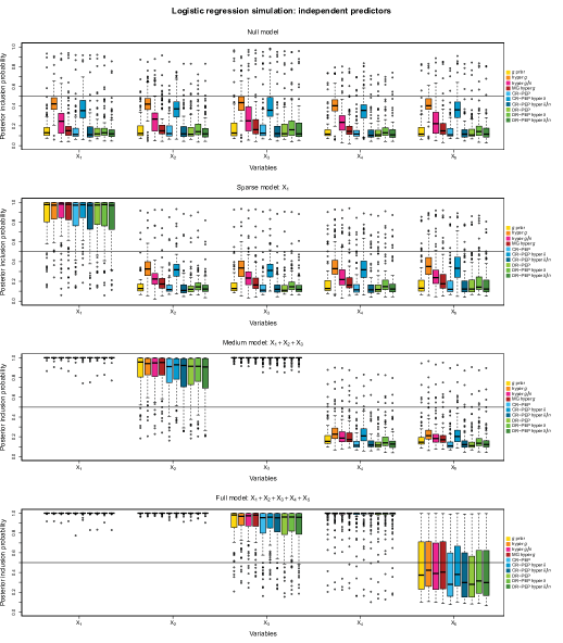
Figure 9: Posterior inclusion probabilities for Simulation Study 1 from 100 replicated samples of the null, sparse, medium and full logistic regression model scenarios with independent predictors ($r=0$).

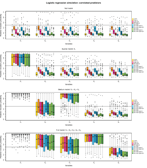
Figure 10: Posterior inclusion probabilities for Simulation Study 1 from 100 replicated samples of the null, sparse, medium and full logistic regression model scenarios with correlated predictors ($r=0.75$).

D.2 Posterior inclusion probabilities (Poisson model)

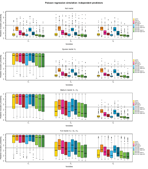
Figure 11: Posterior inclusion probabilities for Simulation Study 1 from 100 replicated samples of the null, sparse, medium and full Poisson model scenarios with independent predictors ($r=0$).

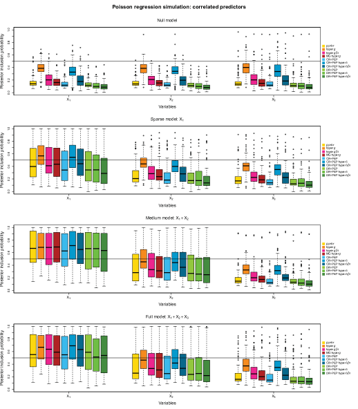
Figure 12: Posterior inclusion probabilities for Simulation Study 1 from 100 replicated samples of the null, sparse, medium and full Poisson model scenarios with correlated predictors ($r=0.75$).

References

- (1)
- Bayarri et al. (2012) Bayarri, M. J., Berger, J. O., Forte, A. and García-Donato, G. (2012), ‘Criteria for Bayesian model choice with application to variable selection’, The Annals of Statistics 40, 1550–1577.
- Berger and Pericchi (1996a) Berger, J. O. and Pericchi, L. R. (1996a), The intrinsic Bayes factor for linear models, in J. Bernardo, J. Berger, A. Dawid, and A. Smith, eds., Bayesian Statistics, Vol. 5, Oxford University Press, pp. 25–44.
- Berger and Pericchi (1996b) Berger, J. O. and Pericchi, L. R. (1996b), ‘The intrinsic Bayes factor for model selection and prediction’, Journal of the American Statistical Association 91, 109–122.
- Bernardo and Smith (2000) Bernardo, J. and Smith, A. (2000), Bayesian Theory, 2nd edition, Wiley, Chichester, UK.
- Casella and Moreno (2006) Casella, G. and Moreno, E. (2006), ‘Objective Bayesian variable selection’, Journal of the American Statistical Association 101, 157–167.
- Chen et al. (2008) Chen, M.-H., Huang, L., Ibrahim, J. G. and Kim, S. (2008), ‘Bayesian variable selection and computation for generalized linear models with conjugate priors’, Bayesian Analysis 3, 585–614.
- Chen and Ibrahim (2003) Chen, M.-H. and Ibrahim, J. G. (2003), ‘Conjugate priors for generalized linear models’, Statistica Sinica 13, 461–476.
- Chen et al. (2000) Chen, M., Ibrahim, J. G. and Shao, Q.-M. (2000), ‘Power prior distributions for generalized linear models’, Journal of Statistical Planning and Inference 84, 121–137.
- Clyde et al. (2011) Clyde, M. A., Ghosh, J. and Littman, M. L. (2011), ‘Bayesian adaptive sampling for variable selection and model averaging’, Journal of Computational and Graphical Statistics 20, 80–101.
- Consonni and Veronese (2008) Consonni, G. and Veronese, P. (2008), ‘Compatibility of prior specifications across linear models’, Statistical Science 23, 332–353.
- Dellaportas et al. (2002) Dellaportas, P., Forster, J. J. and Ntzoufras, I. (2002), ‘On Bayesian model and variable selection using MCMC’, Statistics and Computing 12, 27–36.
- Fouskakis and Ntzoufras (2013) Fouskakis, D. and Ntzoufras, I. (2013), ‘Computation for intrinsic variable selection in normal regression models via expected-posterior prior’, Statistics and Computing 23, 491–499.
- Fouskakis and Ntzoufras (2016) Fouskakis, D. and Ntzoufras, I. (2016), ‘Power-conditional-expected priors: Using -priors with random imaginary data for variable selection’, Journal of Computational and Graphical Statistics (forthcoming); arXiv:1307.2449 [stat.CO] .
- Fouskakis et al. (2015) Fouskakis, D., Ntzoufras, I. and Draper, D. (2015), ‘Power-expected-posterior priors for variable selection in Gaussian linear models’, Bayesian Analysis 10, 75–107.
- Fouskakis et al. (2016) Fouskakis, D., Ntzoufras, I. and Perrakis, K. (2016), ‘Variations of power-expected-posterior priors in normal regression models’, Technical Report (work in progress) .
- Friel and Pettitt (2008) Friel, N. and Pettitt, A. N. (2008), ‘Marginal likelihood estimation via power posteriors’, Journal of the Royal Statistical Society: Series B (Statistical Methodology) 70, 589–607.
- Gupta and Ibrahim (2009) Gupta, M. and Ibrahim, J. G. (2009), ‘An matrix prior for Bayesian analysis in generalized linear models with high dimensional data’, Statistica Sinica 19, 1641–1663.
- Hansen and Yu (2003) Hansen, M. and Yu, B. (2003), ‘Minimum description length model selection criteria for generalized linear models’, Lecture Notes-Monograph Series 6, 145–163.
- Holmes and Held (2006) Holmes, C. C. and Held, L. (2006), ‘Bayesian auxiliary variable models for binary and multinomial regression’, Bayesian Analysis pp. 145–168.
- Ibrahim and Chen (2000) Ibrahim, J. G. and Chen, M.-H. (2000), ‘Power prior distributions for regression models’, Statistical Science 15, 46–60.
- Ibrahim and Laud (1991) Ibrahim, J. G. and Laud, P. W. (1991), ‘On Bayesian analysis of generalized linear models using Jeffreys’s prior’, Journal of the American Statistical Association 86, 981–986.
- Kass and Wasserman (1995) Kass, R. E. and Wasserman, L. (1995), ‘A reference Bayesian test for nested hypotheses and its relationship to the Schwarz criterion’, Journal of the American Statistical Association 90, 928–934.
- Leon-Novelo et al. (2012) Leon-Novelo, L., Moreno, E. and Casella, G. (2012), ‘Objective Bayes model selection in probit models’, Statistics in Medicine 31, 353–365.
- Li and Clyde (2015) Li, Y. and Clyde, M. A. (2015), ‘Mixtures of -priors in generalized linear models’, arXiv:1503.06913v1 [stat.ME] .
- Li and Clyde (2016) Li, Y. and Clyde, M. A. (2016), ‘Mixtures of g -priors in Generalized Linear Models’, arXiv 1503.06913.
- Liang et al. (2008) Liang, F., Paulo, R., Molina, G., Clyde, M. A. and Berger, J. O. (2008), ‘Mixtures of g-priors for Bayesian variable selection’, Journal of the American Statistical Association 103, 410–423.
- Madigan and York (1995) Madigan, D. and York, J. (1995), ‘Bayesian graphical models for discrete data’, International Statistical Review 63, 215–232.
- Maruyama and George (2011) Maruyama, Y. and George, E. I. (2011), ‘Fully Bayes factors with a generalized -prior’, The Annals of Statistics 39, 2740–2765.
- Moreno and Girón (2008) Moreno, E. and Girón, F. J. (2008), ‘Comparison of Bayesian objective procedures for variable selection in linear regression’, Test 17, 472–490.
- Murray et al. (2006) Murray, I., Ghahramani, Z. and MacKay, D. J. C. (2006), MCMC for doubly-intractable distributions, in Proceedings of the 22nd Annual Conference on Uncertainty in Artificial Intelligence, (UAI-06), AUAI Press, pp. 359–366.
- Nott and Kohn (2005) Nott, D. J. and Kohn, R. (2005), ‘Adaptive sampling for Bayesian variable selection’, Biometrika 92, 747–763.
- Ntzoufras et al. (2003) Ntzoufras, I., Dellaportas, P. and Forster, J. J. (2003), ‘Bayesian variable and link determination for generalized linear models’, Journal of Statistical Planning and Inference 111, 165–180.
- Pérez (1998) Pérez, J. (1998), Development of Expected Posterior Prior Distribution for Model Comparisons, PhD thesis, Department of Statistics, Purdue University, USA.
- Pérez and Berger (2002) Pérez, J. M. and Berger, J. O. (2002), ‘Expected-posterior prior distributions for model selection’, Biometrika 89, 491–511.
- Perrakis et al. (2015) Perrakis, K., Fouskakis, D. and Ntzoufras, I. (2015), Bayesian variable selection for generalized linear models using the power-conditional-expected-posterior prior, in S. Frühwirth-Schnatter, A. Bitto, G. Kastner, and A. Posekany, eds., Bayesian Statistics from Methods to Models and Applications: Research from BAYSM 2014, Vol. 126, Springer Proceedings in Mathematics and Statistics, pp. 59–73.
- Ripley (1996) Ripley, B. (1996), Pattern Recognition and Neural Networks, Cambridge University Press, Cambridge.
- Roberts and Rosenthal (2001) Roberts, G. O. and Rosenthal, J. S. (2001), ‘Optimal scaling for various Metropolis- Hastings algorithms’, Statistical Science 16, 351–367.
- Ročková and George (2014) Ročková, V. and George, E. I. (2014), ‘EMVS: The EM Approach to Bayesian variable selection’, Journal of the American Statistical Association 109, 828–846.
- Sabanés Bové and Held (2011) Sabanés Bové, D. and Held, L. (2011), ‘Hyper- priors for generalized linear models’, Bayesian Analysis 6, 387–410.
- Scott and Berger (2010) Scott, J. G. and Berger, J. O. (2010), ‘Bayes and empirical-Bayes multiplicity adjustment in the variable-selection problem’, The Annals of Statistics 38, 2587–2619.
- Wang and George (2007) Wang, X. and George, E. I. (2007), ‘Adaptive Bayesian criteria in variable selection for generalized linear models’, Statistica Sinica 17, 667–690.
- Zellner (1986) Zellner, A. (1986), On assessing prior distributions and Bayesian regression analysis using g-prior distributions, in P. Goel and A. Zellner, eds, ‘Bayesian Inference and Decision Techniques: Essays in Honor of Bruno de Finetti’, North-Holland, Amsterdam, pp. 233–243.
- Zellner and Siow (1980) Zellner, A. and Siow, A. (1980), Posterior odds ratios for selected regression hypothesis (with discussion), In J.M. Bernardo, M.H. DeGroot, D.V. Lindley and A.F.M. Smith, eds., Bayesian Statistics, Vol. 1, Oxford University Press, pp. 585–606 and 618–647 (discussion).