A FOURIER RESTRICTION THEOREM FOR A TWO-DIMENSIONAL SURFACE OF FINITE TYPE

Stefan Buschenhenke, Detlef Müller and Ana Vargas

?abstractname?

The problem of $L^{p}(\mathbbm{R}^{3})\to L^{2}(S)$ Fourier restriction estimates for smooth hypersurfaces $S$ of finite type in $\mathbbm{R}^{3}$ is by now very well understood for a large class of hypersurfaces, including all analytic ones. In this article, we take up the study of more general $L^{p}(\mathbbm{R}^{3})\to L^{q}(S)$ Fourier restriction estimates, by studying a prototypical model class of two-dimensional surfaces for which the Gaussian curvature degenerates in one-dimensional subsets. We obtain sharp restriction theorems in the range given by Tao in 2003 in his work on paraboloids. For high order degeneracies this covers the full range, closing the restriction problem in Lebesgue spaces for those surfaces. A surprising new feature appears, in contrast with the non–vanishing curvature case: there is an extra necessary condition. Our approach is based on an adaptation of the bilinear method. A careful study of the dependence of the bilinear estimates on the curvature and size of the support is required.

1 Introduction

Let $S$ be a smooth hypersurface in $\mathbbm{R}^{n}$ with surface measure $d\sigma_{S}.$ The Fourier restriction problem for $S,$ proposed by by E. M. Stein in the seventies, asks for the range of exponents $p$ and $q$ for which the estimate

$$\bigg{(}\int_{S}|\widehat{f}|^{p}\,d\sigma_{S}\bigg{)}^{1/p}\leq C\|f\|_{L^{q}(\mathbbm{R}^{n})}$$ (1.1)

holds true for every $f\in\mathcal{S}(\mathbbm{R}^{n}),$ with a constant $C$ independent of $f.$ There had been a lot of activity on this problem in the seventies and early eighties. The sharp range in dimension $n=2$ for curves with non-vanishing curvature had been determined through work by C. Fefferman, E. M. Stein and A. Zygmund [F70], [Z74]. In higher dimension, the sharp $L^{q}-L^{2}$ result for hypersurfaces with non-vanishing Gaussian curvature was obtained by E. M. Stein and P. A. Tomas [To75], [St86] (see also Strichartz [Str77]). Some more general classes of surfaces were treated by A. Greenleaf [Gr81].

The question about the general $L^{q}-L^{p}$ restriction estimates is nevertheless still wide open. Fundamental progress has been made since the nineties, with contributions by many. Major new ideas were introduced in particular by J. Bourgain (see for instance [Bo91], [Bo95a]) and T. Wolff ([W95]), which led to important further steps towards an understanding of the case of non-vanishing Gaussian curvature. These ideas and methods were further developed by A. Moyua, A. Vargas, L. Vega and T. Tao ([MVV96], [MVV99] [TVV98]), who established the so-called bilinear approach (which had been anticipated in the work of C. Fefferman [F70] and had implicitly been present in the work of J. Bourgain [Bo95b]) for hypersurfaces with non-vanishing Gaussian curvature for which all principal curvatures have the same sign. The same method was applied to the light cone by Tao-Vargas (see [TVI00], [TVII00]). The climax of the application of that bilinear method to these types of surfaces is due to T. Tao [T01b] (for principal curvatures of the same sign), and T. Wolff [W01] and T. Tao [T01a] (for the light cone). In particular, in these last two papers the sharp linear restriction estimates for the light cone in $\mathbbm{R}^{4}$ were obtained.

For the case of non-vanishing curvature but principal curvatures of different signs, analogous results in $\mathbbm{R}^{3}$ were proved by S. Lee [L05] and A. Vargas [V05]. Results for the light cone were previously obtained in $\mathbbm{R}^{3}$ by B. Barceló [Ba85], who also considered more general cones [Ba86]. These results were improved to sharp theorems by S. Buschenhenke [Bu15]. The bilinear approach also produced results for hypersurfaces with $k\leq n-2$ non-vanishing principal curvatures ([LV10]).

More recently, J. Bourgain and L. Guth [BoG11] made further important progress on the case of non-vanishing curvature by making use also of multilinear restriction estimates due to J. Bennett, A. Carbery and T. Tao [BCT06].

On the other hand, general finite type surfaces in $\mathbbm{R}^{3}$ (without assumptions on the curvature) have been considered in work by I. Ikromov, M. Kempe and D. Müller [IKM10] and Ikromov and Müller [IM11], [IM15], and the sharp range of Stein-Tomas type $L^{q}-L^{2}$ restriction estimates has been determined for a large class of smooth, finite-type hypersurfaces, including all analytic hypersurfaces.

It is our aim in this work to take up the latter branch of development by considering a certain model class of hypersurfaces in dimension three with varying curvature and study more general $L^{q}-L^{p}$ restriction estimates. Our approach will again be based on the bilinear method. In our model class, the degeneracy of the curvature will take place along one-dimensional subvarieties. For analytic hypersurfaces whose Gaussian curvature does not vanish identically, this kind of behavior is typical, even though in our model class the zero varieties will still be linear (or the union of two linear subsets). Even though our model class would seem to be among the simplest possible surfaces of such behavior, we will see that they require a very intricate study. We hope that this work will give some insight also for future research on more general types of hypersurfaces.

Independently of our work, a result for rotationally invariant surfaces with degeneracy of the curvature at a single point has been obtained recently by B. Stovall [Sto15].

1.1 Outline of the problem. The adjoint setting

We start with a description of the surfaces that we want to study. We will consider surfaces that are graps of smooth functions defined on $Q=]0,1[\times]0,1[,$

$$\Gamma=\text{\rm graph\,}(\phi)=\{(\xi,\phi(\xi)):\xi\in Q\}.$$

The surface $\Gamma$ is equipped with the surface measure, $\sigma_{\Gamma}.$ It will be more convenient to use duality and work in the adjoint setting. The adjoint restriction operator is given by

$$\mathcal{R}^{\ast}f(x)=\widehat{f\,d\sigma_{\Gamma}}(x)=\int_{\Gamma}f(\xi)e^{-ix\cdot\xi}\,d\sigma_{\Gamma}(\xi),$$ (1.2)

where $f\in L^{q}(\Gamma,\sigma_{\Gamma}).$ The restriction problem is therefore equivalent to the question of finding the appropriate range of exponents for which the estimate

$$\|\mathcal{R}^{*}f\|_{L^{p}(\mathbbm{R}^{3})}\leq C\|f\|_{L^{q}(\Gamma,d\sigma_{\Gamma})},$$

holds with a constant $C$ independent of the function $f\in L^{q}(\Gamma,d\sigma_{s}).$ We shall require the following properties of the functions $\phi:$

Let $m_{1},m_{2}\in\mathbbm{R}$, $m_{1},m_{2}\geq 2$. We say that a function $\phi$ is of normalized type $(m_{1},m_{2})$ if there exists $\psi_{1},\psi_{2}\in C^{\infty}(]0,1[)$ and $a,b>0$ such that

$$\phi(\xi_{1},\xi_{2})=\psi_{1}(\xi_{1})+\psi_{2}(\xi_{2})$$ (1.3)

on $]0,1[\times]0,1[,$ where the derivatives of the $\psi_{i}$ satisfy

$$\psi_{i}^{\prime\prime}(\xi_{i}) \sim\xi_{i}^{m_{i}-2},$$ (1.4)

$$|\psi_{i}^{(k)}(\xi_{i})| \lesssim\xi_{i}^{m_{i}-k}\quad\mbox{for }\ k\geq 3.$$ (1.5)

The constants hidden in these estimates are assumed to be admissible in the sense that they only depend on $m_{1},m_{2}$ and the order of the derivative, but not explicitly on the $\psi_{i}$’s.

One would of course expect that small perturbations of such functions $\phi,$ depending on both $\xi_{1}$ and $\xi_{2},$ should lead to hypersurfaces sharing the same restriction estimates as our model class above. However, such perturbation terms are not covered by our proof. It seems that the treatment of these more general situations would require even more intricate arguments, which will have to take the underlying geometry of the surface into account. We plan to study these questions in the future.

The prototypical example of of a normalized function of type $(m_{1},m_{2})$ is of course $\phi(\xi)=\xi_{1}^{m_{1}}+\xi_{2}^{m_{2}}.$ For $m_{1}$ and $m_{2}$ integer, others arise simply as follows:

Remarks 1.1.

1. Let $\varepsilon>0$ and $\varphi\in C^{\infty}(]-\varepsilon,\varepsilon[)$ be of finite type $m\in\mathbbm{N}$ in $0$, i.e., $\varphi(0)=\varphi^{\prime}(0)=\cdots=\varphi^{(m-1)}(0)=0\neq\varphi^{(m)}(0)$. Assume $\varphi^{(m)}(0)>0$. Then there exist $\varepsilon^{\prime}\in(0,\varepsilon)$ such that

   $$\varphi^{(k)}(t)\sim t^{m-k}$$

   for all $0\leq k\leq m$, $|t|<\varepsilon^{\prime}$.

2. Further let $\phi(\xi)=\psi_{1}(\xi_{1})+\psi_{2}(\xi_{2})$, $|\xi|\leq\varepsilon$, where $\psi_{i}\in C^{\infty}(]-\varepsilon,\varepsilon[)$ is of finite type $m_{i}$ in $0$ with $\varphi_{i}^{(m_{i})}(0)>0$. Then there exist an $\bar{\varepsilon}>0$ such that $y\mapsto\phi(\bar{\varepsilon}y)$ is of normalised finite type $(m_{1},m_{2})$.

Proof:.

(i) Since $\varphi$ has a zero of order $m$ at the origin, we find some $\varepsilon_{0}>0$, a smooth function $\chi_{0}:]-\varepsilon_{0},\varepsilon_{0}[\to]0,\infty[$ and a sign $\sigma=\pm 1$ such that

$$\varphi(t)=\sigma t^{m}\chi_{0}(t)$$

for all $|t|<\varepsilon_{0}$. Thus $\varphi^{\prime}(t)=\sigma t^{m-1}[m\chi_{0}(t)+t\chi_{0}^{\prime}(t)]$. Since $\chi_{0}^{\prime}$ is bounded on any compact neighborhood of the origin, and $\chi_{0}$ is bounded from below by a positive constant if the neighborhood is small enough, we have $t\chi_{0}^{\prime}(t)\ll m\chi_{0}(t)$ for $t$ small enough, and thus we find $0<\varepsilon_{1}<\varepsilon_{0}$ such that

$$\varphi^{\prime}(t)=\sigma t^{m-1}\chi_{1}(t),$$

where $\chi_{1}(t)=m\chi_{0}(t)+t\chi_{0}^{\prime}(t)>0$ for all $|t|\leq\varepsilon_{1}$. Iterating the procedure gives $\varepsilon_{k}>0$, $\chi_{k}:]-\varepsilon_{k},\varepsilon_{k}[\to]0,\infty[$ such that

$$\varphi^{(k)}(t)=\sigma t^{m-k}\chi_{k}(t)$$

for every $|t|<\varepsilon_{k}$. Finally observe that $0<\varphi^{(m)}(0)=\sigma\chi_{m}(0)$, i.e., $\sigma=1$.

(ii) Chose $\bar{\varepsilon}>0$ such that for both $i=1,2$, $0\leq k\leq m_{i}$ and all $0\leq t\leq\bar{\varepsilon}$

$$\varphi^{(k)}_{i}(t)\sim t^{(m_{i}-k)}.$$

Then for all $0\leq s\leq 1$

$$\frac{d^{k}}{ds^{k}}\varphi_{i}(\bar{\varepsilon}s)\sim\bar{\varepsilon}^{k}(\bar{\varepsilon}s)^{(m_{i}-k)}=\bar{\varepsilon}^{m_{i}}s^{(m_{i}-k)}.$$

$\Box$

In order to formulate our main theorem, adapting Varchenko’s notion of height to our setting, we introduce the height $h$ of the surface by

$$\frac{1}{h}=\frac{1}{m_{1}}+\frac{1}{m_{2}}.$$

Let us also put put $\bar{m}=m_{1}\vee m_{2}=\max\{m_{1},m_{2}\}$ and $m=m_{1}\wedge m_{2}=\min\{m_{1},m_{2}\}$.

Theorem 1.2.

Let $p>\max\{\frac{10}{3},h+1\}$, $\frac{1}{s^{\prime}}\geq\frac{h+1}{p}$ and $\frac{1}{s}+\frac{2\bar{m}+1}{p}<\frac{\bar{m}+2}{2}$. Then $\mathcal{R}^{*}$ is bounded from $L^{s,t}(\Gamma,d\sigma_{\Gamma})$ to $L^{p,t}(\mathbbm{R}^{3})$ for every $1\leq t\leq\infty$.

If in addition $s\leq p$ or $\frac{1}{s^{\prime}}>\frac{h+1}{p},$ then $\mathcal{R}^{*}$ is even bounded from $L^{s}(\Gamma,d\sigma_{\Gamma})$ to $L^{p}(\mathbbm{R}^{3})$.

Remarks 1.3.

1. Notice that the “critical line” ${1}/{s^{\prime}}={(h+1)}/{p}$ and the line ${1}/{s}+{(2\bar{m}+1)}/{p}={(\bar{m}+2)}/{2}$ in the $(1/s,1/p)$-plane intersect at the point $(1/s_{0},1/p_{0})$ given by

   $$\frac{1}{s_{0}}=\frac{3\bar{m}+m-m\bar{m}}{4\bar{m}+2m},\quad\frac{1}{p_{0}}=\frac{\bar{m}+m}{4\bar{m}+2m}.$$ (1.6)

   This shows in particular that the point $(1/s_{0},1/p_{0})$ lies strictly above (if $m>2$) or on the bi-sectrix $1/s=1/p$ (if $m=2$).

2. The condition $1/{s^{\prime}}\geq{(h+1)}/{p}$ in the theorem is necessary and in fact dictated by homogeneity (Knapp box examples).

3. By (i), the condition

   $$\frac{\bar{m}+2}{2}>\frac{2\bar{m}+1}{p}+\frac{1}{s}$$ (1.7)

   only plays a role above the bi-sectrix. It is necessary too when $p<s,$ hence, in view of (i), if $m>2,$ and if $m=2,$ it is necessary with the possible exception of the case where $s_{0}=p_{0}=4(\bar{m}+1)/(\bar{m}+2),$ for which we do not have an argument. Our proof in Section 1.3 will reflect the fact that for $m_{j}>2,$ the behavior of the operator must be worse than for the case $m_{j}=2.$

4. From the first condition in the theorem, we see that $p\geq h+1$ is also necessary. Moreover, we shall show in Section 1.3 that strong type estimates are not possible unless $s\leq p$ or ${1}/{s^{\prime}}>{(h+1)}/{p}.$ The condition $p>{10}/3$ is due to the use of the bilinear method, as this exponent gives the sharp bilinear result for the paraboloid, and it is surely not sharp. Nevertheless, when $h>7/3,$ we obtain the sharp result.

A new phenomenon appears in these surfaces. In the case of non-vanishing Gaussian curvature, it is conjectured that the sharp range is given by the homogeneity condition $1/{s^{\prime}}\geq{(h+1)}/{p}$ (with $h=2/(n-1),$ hence $h+1=(n+1)/(n-1)$), and a second condition, $p>{2n}/{(n-1)},$ due to the decay rate of the Fourier transform of the surface measure. A similar result is conjectured for the light cone (cf. Figure 1).

?figurename? 1: Conjectured range of $p$ and $q$ for nonvanishing Gaussian curvature

In contrast to this, we show in our theorem that for the class of surfaces $\Gamma$ under consideration a third condition appears, namely (1.7).

Let us briefly discuss the different situations that may arise in Theorem 1.2, depending on the choice of $m_{1}$ and $m_{2}:$

First observe that $1/p_{0}$ in (1.6) is above the critical threshold $1/{p_{c}}={3}/{10}$, if $\bar{m}\leq 2m$. In this case, the new condition ${1}/{s}+{(2\bar{m}+1)}/{p}={(\bar{m}+2)}/{2}$ will not show up in our theorem. So for $\bar{m}\leq 2m$, we are in the situation of either Figure 2 (if $h\leq{7}/{3}$, i.e., $h+1\leq{10}/{3}$) or of Figure 3 (if $h>{7}/{3}$). Notice that in the last case our theorem is sharp.

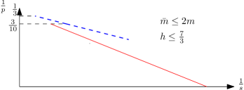
?figurename? 2: Range of $p$ and $s$ in Theorem 1.2

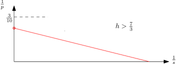
?figurename? 3: Range of $p$ and $s$ in Theorem 1.2

It might also be interesting to compare $p_{0}$ not only with the condition $p>{10}/{3}$, which is due to the bilinear method, but with the conjectured range $p>3$. We always have $p_{0}\geq 3$, while we have $p_{0}=3$ only if $m_{1}=m_{2}$, i.e., a reasonable conjecture is that the new condition (1.7) should always appear for inhomogeneous surfaces with $m_{1}\neq m_{2}$. In the case $\bar{m}>2m$, our new condition might be visible. Observe next that the line ${1}/{s}+{(2\bar{m}+1)}/{p}={(\bar{m}+2)}/{2}$ intersects the ${1}/{p}$-axis where $p=p_{1}={(4\bar{m}+2)}/{(\bar{m}+2)}$. Thus there are two subcases:

For $\bar{m}<7$ we have $p_{1}<{10}/{3}$, corresponding to Figure 4, and our new condition appears.

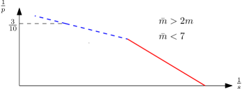
?figurename? 4: Range of $p$ and $s$ in Theorem 1.2

For $\bar{m}\geq 7$ we may either have $p_{0}\geq p_{1}\geq h+1$ (which is equivalent to $\bar{m}m\geq 3\bar{m}+m$) and thus Figure 5 applies, or $p_{0}<p_{1}<h+1$ (which is equivalent to $\bar{m}m<3\bar{m}+m$), and we are in the situation of Figure 3; here again the new condition becomes relevant. Observe that in the two last mentioned cases, i.e., for $\bar{m}\geq 7$, our theorem is always sharp.

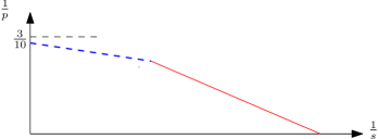
?figurename? 5: Range of $p$ and $s$ in Theorem 1.2

Further observe that the appearance of a third condition, besides the classical ones, is natural: Fix $m_{1}=2$ and let $\bar{m}=m_{2}\to\infty.$ Then the contact order in the second coordinate direction degenerates. Hence, we would expect to find the same $p$-range as for a two dimensional cylinder, which agrees with the range for a parabola in the plane, namely $p>4$ (see [F70], [Z74]). Since $h\to 2$ as $\bar{m}=m_{2}\to\infty,$ the condition $p>\max\{{10}/{3},h+1\}$ becomes $p>{10}/{3}$ in the limit, which would lead to a larger range than expected. However, the new extra condition $1/s+{(2\bar{m}+1)}/{p}<{(\bar{m}+2)}/{2}$ becomes $p>4$ for $\bar{m}\to\infty,$ as is to be expected.

The restriction problem for the graph of functions $\phi(x)=\xi_{1}^{m_{1}}+\xi_{2}^{m_{2}}$ (and related surfaces) had previously already been studied by E. Ferreyra and M. Urciuolo [FU09], however by simpler methods, which led to weaker results than ours. In their approach, they made use of the invariance of this surface under suitable non-isotropic dilations as well as of the one-dimensional results for curves. This allowed them to obtain some results for $p>4,$ in the region below the homogeneity line, i.e., for ${1}/{s^{\prime}}>(h+1)/{p}.$ Our results are stronger in two ways: they include the critical line and, more importantly, when $h<3,$ we obtain a larger range for $p.$

As for the points on the critical line in the range $p>4,$ let us indicate that these points can in fact also be obtained by means of a simple summation argument involving Lorentz spaces and real interpolation. This can be achieved by means of summation trick going back to ideas by Bourgain [Bou85] (see for instance [TVV98], [L03]). Details are given in Section 7.1 of this article.

1.2 Passage from surface to Lebesgue measure

We shall always consider hypersurfaces $S=\{(\eta,\phi(\eta)):\eta\in U\}$ which are the graphs of functions $\phi$ that are smooth on an open bounded subset $U\subset\mathbbm{R}^{d}$ and continuous on the closure of $U.$ The adjoint of the Fourier restriction operator associated to $S$ is then given by

$$\mathcal{R}^{\ast}f(x,t)=\widehat{f\,d\sigma_{S}}(x,t)=\int_{S}f(\xi)e^{-i(x,t)\cdot\xi}\,d\sigma_{S}(\xi),\qquad(x,t)\in\mathbbm{R}^{d}\times\mathbbm{R}=\mathbbm{R}^{d+1},$$

where $d\sigma_{S}=(1+|\nabla\phi(\eta)|^{2})^{1/2}\,d\eta$ denotes the Riemannian surface measure of $S.$ Here, $f:S\to\mathbbm{C}$ is a function on $S,$ but we shall often identify it with the corresponding function $\tilde{f}:U\to\mathbbm{C},$ given by $\tilde{f}(\eta)=f(\eta,\phi(\eta)).$ Correspondingly, we define

$$R^{*}_{\mathbbm{R}^{d}}g(x,t):=\widehat{gd\nu}(x,t):=\int_{U}g(\eta)e^{-i(x\eta+t\phi(\eta))}\,d\eta,\qquad(x,t)\in\mathbbm{R}^{d}\times\mathbbm{R}=\mathbbm{R}^{d+1},$$

for every function $g\in L^{1}(U)$ on $U.$ We shall occasionally address $d\nu=d\nu_{S}$ as the “Lebesgue measure” on $S,$ in contrast with the surface measure $d\sigma=d\sigma_{S}.$ Moreover, to emphasize which surface $S$ is meant, we shall occasionally also write $R^{*}_{\mathbbm{R}^{d}}=R^{*}_{S,\mathbbm{R}^{d}}.$ Observe that if there is a constant $A$ such that

$$|\nabla\phi(\eta)|\leq A,\qquad\eta\in U,$$ (1.8)

(this applies for instance to our class of hypersurfaces $\Gamma,$ since we assume that $m_{i}\geq 2$), then the Lebesgue measure $d\nu$ and the surface measure $d\sigma$ are comparable, up to some positive multiplicative constants depending only on $A.$ Moreover, since

$$R^{\ast}f=R^{*}_{\mathbbm{R}^{d}}\big{(}\tilde{f}(1+|\nabla\phi(\eta)|^{2})^{1/2}\big{)},$$ (1.9)

the $L^{q}$-norms $\|\tilde{f}\|_{L^{q}(d\eta)}$ and $\|f\|_{L^{q}(d\sigma_{S})}=\|\tilde{f}(1+|\nabla\phi(\eta)|^{2})^{1/2q}\|_{L^{q}(d\eta)}$ of $\tilde{f}$ and of $f$ are comparable too. Throughout the article, we shall therefore apply the following

Convention 1.4.

Whenever $|\nabla\phi|\lesssim 1,$ then, with some slight abuse of notation, we shall denote the function $f$ on $S$ and the corresponding function $\tilde{f}$ on $U$ by the same symbol $f,$ and write $R_{\mathbbm{R}^{d}}^{*}f$ in place of $R_{\mathbbm{R}^{d}}^{*}\tilde{f}.$

Applying this in particular to the hypersurfaces $\Gamma,$ we see that Theorem 1.2 is equivalent to the following

Theorem 1.5.

Let $p>\max\{\frac{10}{3},h+1\}$, $\frac{1}{s^{\prime}}\geq\frac{h+1}{p}$ and $\frac{1}{s}+\frac{2\bar{m}+1}{p}<\frac{\bar{m}+2}{2}$. Then $R_{\mathbbm{R}^{2}}^{*}$ is bounded from $L^{s,t}(\Gamma,d\sigma_{\Gamma})$ to $L^{p,t}(\mathbbm{R}^{3})$ for every $1\leq t\leq\infty$.

If in addition $s\leq p$ or $\frac{1}{s^{\prime}}>\frac{h+1}{p},$ then $R_{\mathbbm{R}^{2}}^{*}$ is even bounded from $L^{s}(\Gamma,d\sigma_{\Gamma})$ to $L^{p}(\mathbbm{R}^{3})$.

1.3 Necessary conditions

The condition $p>h+1$ is in some sense the weakest one. Indeed, the second condition already implies $p\geq h+1,$ and even $p>h+1$ when $s<\infty.$ Thus the condition $p>h+1$ only plays a role when the critical line ${1}/{s^{\prime}}={(h+1)}/{p}$ intersects the axis ${1}/{s}=0$ at a point where $p>p_{c}=10/3$ (cf. Figure 3).

However, the condition $p>h+1$ is necessary as well (although some kind of weak type estimate might hold true at the endpoint). This can be shown by analyzing the oscillatory integral defined by $R^{*}_{\mathbbm{R}^{d}}1$ (compare [S87] for similar arguments). For the sake of simplicity, we shall do this only for the model case $\phi(\xi)=\xi_{1}^{m_{1}}+\xi_{2}^{m_{2}}$ (the more general case can be treated by similar, but technically more involved arguments).

Indeed, we have the following well-known lower bounds on related oscillatory integrals (for the convenience of the reader, we include a proof):

Lemma 1.6.

Assume that $m\geq 2.$

1. If $1\ll\mu\ll\lambda\ll\mu^{m}$, then $\left|\int_{0}^{\delta}e^{i(\mu\xi-\lambda(\xi^{m}+\mathcal{O}(\xi^{m+1}))}{d}\xi\right|\geq C_{\delta}\mu^{-\frac{m-2}{2m-2}}\lambda^{-\frac{1}{2m-2}}$, provided $\delta>0$ is sufficiently small.

2. If $1\ll\mu^{m}\ll\lambda,$ $0\leq\alpha<1$ and $0\leq\beta<1$ , then

   $$\left|\int_{0}^{1}e^{i(\mu\xi-\lambda\xi^{m})}\xi^{-\alpha}|\log(\xi/2)|^{-\beta}d\xi\right|\gtrsim\lambda^{\frac{\alpha-1}{m}}(\log\lambda)^{-\beta}.$$

Proof:.

(i) Apply the transformation $\xi\mapsto\left({\mu}/{\lambda}\right)^{\frac{1}{m-1}}\xi$ to obtain

$$\int_{0}^{\delta}e^{i(\mu\xi-\lambda\xi^{m}+\mathcal{O}(\xi^{m+1}))}{d}\xi =\int_{0}^{\delta\left(\frac{\lambda}{\mu}\right)^{\frac{1}{m-1}}}\left(\frac{\mu}{\lambda}\right)^{\frac{1}{m-1}}e^{i\left(\frac{\mu^{m}}{\lambda}\right)^{\frac{1}{m-1}}\big{(}\xi-\xi^{m}+\mathcal{O}((\frac{\mu}{\lambda})^{\frac{1}{m-1}}\xi^{m+1})\big{)}}{d}\xi$$

$$=\int_{0}^{1}+\int_{1}^{\delta\left(\frac{\lambda}{\mu}\right)^{\frac{1}{m-1}}},$$

where $\left({\mu}/{\lambda}\right)^{\frac{1}{m-1}}\ll 1$ and $\left({\mu^{m}}/{\lambda}\right)^{\frac{1}{m-1}}\gg 1$. The phase function $\phi(\xi)=\xi-\xi^{m}+\mathcal{O}((\frac{\mu}{\lambda})^{\frac{1}{m-1}}\xi^{m+1})$ has a unique critical point at $\xi_{0}=\xi_{0}(\mu/\lambda)$ in $[0,1]$ lying very close to $m^{-1/(m-1)}$ , so we may apply the method of stationary phase to the first integral and find that

$$\left|\int_{0}^{1}\right|\gtrsim\left(\frac{\mu}{\lambda}\right)^{\frac{1}{m-1}}\left(\frac{\mu^{m}}{\lambda}\right)^{-\frac{1}{2}\frac{1}{m-1}}.$$

Moreover, integration by parts in the second integral leads to

$$\left|\int_{1}^{\delta\left(\frac{\lambda}{\mu}\right)^{\frac{1}{m-1}}}\right|\lesssim C_{1}\left(\frac{\mu}{\lambda}\right)^{\frac{1}{m-1}}\left(\frac{\mu^{m}}{\lambda}\right)^{-\frac{1}{m-1}},$$

provided $\delta$ is sufficiently small. These estimates imply that

$$\left|\int_{0}^{1}\left(\frac{\mu}{\lambda}\right)^{\frac{1}{m-1}}e^{i(\mu\xi-\lambda\xi^{m}+\mathcal{O}(\xi^{m+1}))}{d}\xi\right|\gtrsim\left(\frac{\mu}{\lambda}\right)^{\frac{1}{m-1}}\left(\frac{\mu^{m}}{\lambda}\right)^{-\frac{1}{2}\frac{1}{m-1}}=\mu^{-\frac{m-2}{2m-2}}\lambda^{-\frac{1}{2m-2}}.$$

(ii) Apply the change of variables $\xi\mapsto\lambda^{-\frac{1}{m}}\xi$ to obtain

$$\left|\int_{0}^{1}e^{i(\mu\xi-\lambda\xi^{m})}\xi^{-\alpha}|\log(\xi/2)|^{-\beta}{d}\xi\right|$$

$$= \lambda^{\frac{\alpha-1}{m}}|\log(\lambda^{-\frac{1}{m}})|^{-\beta}\left|\int_{0}^{\lambda^{\frac{1}{m}}}e^{i(\mu\lambda^{-\frac{1}{m}}\xi-\xi^{m})}\xi^{-\alpha}\Big{(}1+\frac{|\log(\xi/2)|}{\frac{1}{m}\log\lambda}\Big{)}^{-\beta}\,{d}\xi\right|$$

$$\gtrsim \lambda^{\frac{\alpha-1}{m}}(\log\lambda)^{-\beta}.$$

Notice here that $\lambda^{1/m}\gg 1$ and $\mu\lambda^{-\frac{1}{m}}\ll 1,$ and that, as $\lambda\to\infty,$ the last oscillatory integral tends to $\int_{0}^{\infty}e^{-i\xi^{m}}\xi^{-\alpha}{d}\xi\neq 0$ (which is easily seen). $\Box$

Part (ii) of the lemma implies that

$$\left|\int_{0}^{1}e^{-i(x_{1}\xi-x_{3}\xi^{m_{1}})}d\xi\right|\gtrsim x_{3}^{-\frac{1}{m_{1}}}$$

for $1\leq x_{3}<\infty$, $1\ll x_{1}^{m_{1}}\ll x_{3},$ and since $R^{*}_{\mathbbm{R}^{d}}1=\widehat{d\nu},$ we find that

$$\|R^{*}_{\mathbbm{R}^{d}}1\|_{p}^{p}\geq \int_{1}^{\infty}\int_{1\ll x_{2}\ll x_{3}^{\frac{1}{m_{2}}}}\int_{1\ll x_{1}\ll x_{3}^{\frac{1}{m_{1}}}}|R^{*}_{\mathbbm{R}^{d}}1(x_{1},x_{2},-x_{3})|^{p}dx_{1}dx_{2}dx_{3}$$

$$\gtrsim \int_{1}^{\infty}\int_{1\ll x_{2}\ll x_{3}^{\frac{1}{m_{2}}}}dx_{2}\int_{1\ll x_{1}\ll x_{3}^{\frac{1}{m_{1}}}}dx_{1}x_{3}^{-p\left(\frac{1}{m_{1}}+\frac{1}{m_{2}}\right)}dx_{3}$$

$$\gtrsim \int_{1}^{\infty}x_{3}^{(1-p)\left(\frac{1}{m_{1}}+\frac{1}{m_{2}}\right)}dx_{3}$$

$$= \int_{1}^{\infty}x_{3}^{-\frac{p-1}{h}}dx_{3}.$$

If the adjoint Fourier restriction operator is bounded, the integral has to be finite, thus necessarily ${(p-1)}/{h}>1$, i.e., $p>h+1.$

Next, to see that the condition (1.7), i.e., ${(\bar{m}+2)}/{2}>{(2\bar{m}+1)}/{p}+{1}/{s},$ is necessary in Theorem 1.2, we consider the subsurface

$$\Gamma_{0}=\{(\xi,\phi(\xi)):\xi\in[0,1]\times[1/2,1/2+\delta]\},$$

where $\delta>0$ is assumed to be sufficiently small. On this subsurface, the principal curvature in the $\xi_{2}$-direction is bounded from below. This means that, after applying a suitable affine transformation of coordinates, the restriction problem for the surface $\Gamma_{0}$ is equivalent to the one for the surface

$$\Gamma_{m_{1},2}=\{(\xi_{1},\xi_{2},\xi_{1}^{m_{1}}+c(\xi_{2}^{2}+\mathcal{O}(\xi_{2}^{3}))):(\xi_{1},\xi_{2})\in[0,1]\times[0,\delta]\},$$

where $c>0.$

As stated in Remark 1.3, the condition (1.7) only plays a role above the bi-sectrix $1/s=1/p$. So, assume that $p<s$ (as explained, this excludes only the case where $m=2$ and $s=p=p_{0}$). Then we may choose $\beta<1$ such that $\beta s>1>\beta p.$ Assume that $\mathcal{R}^{\ast}_{\Gamma}$ is bounded from $L^{s}(\Gamma)$ to $L^{p}(\mathbbm{R}^{3})$, i.e., $\mathcal{R}^{\ast}_{\Gamma_{m_{1},2}}$ is bounded from $L^{s}(\Gamma_{m_{1},2})$ to $L^{p}(\mathbbm{R}^{3})$. Passing again from the surface measure $d\sigma$ to the “Lebesgue measure” $d\nu$ on $\Gamma_{m_{1},2},$ define $f(\xi_{1},\xi_{2})=\xi_{1}^{-{1}/{s}}\log(\xi_{1}/2)^{-\beta}\in L^{s}(\Gamma_{m_{1},2},d\nu).$ Then

$$|\widehat{f{d}\nu}(x_{1},x_{2},-t)|= \left|\int_{[0,1]\times[0,\delta]}e^{i(x_{1}\xi_{1}+x_{2}\xi_{2}-t(\xi_{1}^{m_{1}}+c(\xi_{2}^{2}+\mathcal{O}(\xi_{2}^{3})))}\xi_{1}^{-\frac{1}{s}}\log(\xi_{1}/2)^{-\beta}{d}(\xi_{1},\xi_{2})\right|$$

$$= \left|\int_{0}^{1}e^{i(x_{1}\xi_{1}-t\xi_{1}^{m_{1}})}\xi_{1}^{-\frac{1}{s}}\log(\xi_{1}/2)^{-\beta}{d}\xi_{1}\right|\ \left|\int_{0}^{\delta}e^{i(x_{2}\xi_{2}-tc(\xi_{2}^{2}+\mathcal{O}(\xi_{2}^{3}))}{d}\xi_{2}\right|.$$

We estimate the first integral by means of Lemma 1.6 (ii), and for the second one we use Lemma 1.6 (i) (with $m=2$), which leads to

$$\infty>\|f\|_{s}^{p}\gtrsim\|\widehat{f{d}\nu}\|_{p}^{p}\gtrsim \int_{N}^{\infty}\int_{t^{1/2}}^{t}\int_{1}^{t^{\frac{1}{m_{1}}}}t^{-\frac{p}{s^{\prime}m_{1}}}t^{-\frac{p}{2}}(\log t)^{-\beta p}\,dx_{1}dx_{2}dt$$

$$\approx \int_{N}^{\infty}t^{1-\frac{p}{2}}t^{\frac{1}{m_{1}}-\frac{p}{s^{\prime}m_{1}}}(\log t)^{-\beta p}\,dt,$$

provided $N$ is chosen sufficiently large. This implies that necessarily

$$1-\frac{p}{2}+\frac{1}{m_{1}}-\frac{p}{s^{\prime}m_{1}}<-1,$$

which is equivalent to

$$\frac{m_{1}+2}{2}>\frac{2m_{1}+1}{p}+\frac{1}{s}.$$

Interchanging the roles of $\xi_{1}$ and $\xi_{2}$, we obtain the same inequality for $m_{2}$ and hence for $\bar{m}=m_{1}\vee m_{2}$, and we arrive at (1.7).

Let us finally prove that on the critical line $1/s^{\prime}=(h+1)/p$ one cannot have strong-type estimates above the bi-sectrix $1/s=1/p$, i.e., for $s>p$. In this regime, we find some $1>r>0$ such that $1/s<r<1/p$. Let

$$f(\xi)=\xi_{2}^{-m_{2}/sh}|\log(\xi_{2}/2)|^{-r}\chi_{\{\xi_{1}^{m_{1}}\leq\xi_{2}^{m_{2}}\}}(\xi).$$

It is easy to check that $f\in L^{s}(\Gamma)$ since $1<rs$. Now assume that $1\ll x_{j}^{m_{j}}\ll t$ for $j=1,2,$ more precisely choose $N\gg 1$ and assume that $N^{2}\leq Nx_{j}^{m_{j}}\leq t$ for $j=1,2$. Then

$$(R^{*}_{\mathbbm{R}^{d}}f)(x_{1},x_{2},-t) =\int_{0}^{1}e^{-i(x_{2}\xi_{2}-t\xi_{2}^{m_{2}})}\xi_{2}^{-m_{2}/sh}|\log(\xi_{2}/2)|^{-r}$$

$$\qquad\times\int_{0}^{\xi_{2}^{m_{2}/m_{1}}}e^{-i(x_{1}\xi_{1}-t\xi_{1}^{m_{1}})}d\xi_{1}d\xi_{2}.$$

Since $x_{1}^{m_{1}}\ll t$ is equivalent to $(\xi_{2}^{m_{2}/m_{1}}x_{1})^{m_{1}}\ll t\xi_{2}^{m_{2}}$, Lemma 1.6 (ii) gives

$$\left|\int_{0}^{\xi_{2}^{m_{2}/m_{1}}}e^{-i(x_{1}\xi_{1}-t\xi_{1}^{m_{1}})}d\xi_{1}\right|=\xi_{2}^{\frac{m_{2}}{m_{1}}}\left|\int_{0}^{1}e^{-i(\xi_{2}^{m_{2}/m_{1}}x_{1}\eta-t\xi_{2}^{m_{2}}\eta^{m_{1}})}d\eta\right|\gtrsim t^{-\frac{1}{m_{1}}}.$$

Applying Lemma 1.6 once more, we obtain

$$\left|(R^{*}_{\mathbbm{R}^{d}}f)(x_{1},x_{2},-t)\right|\gtrsim t^{-\frac{1}{m_{1}}}t^{\frac{1}{sh}-\frac{1}{m_{2}}}\log^{-r}(t/2)=t^{-\frac{1}{p}\left(1+\frac{1}{h}\right)}\log^{-r}(t/2),$$

where we made use of $1/s^{\prime}=(h+1)/p$. Thus we get

$$\|R^{*}_{\mathbbm{R}^{d}}f\|_{p}^{p}\gtrsim \int_{N^{2}}^{\infty}\int_{N^{\frac{1}{m_{2}}}}^{(t/N)^{\frac{1}{m_{2}}}}\int_{N^{\frac{1}{m_{1}}}}^{(t/N)^{\frac{1}{m_{1}}}}t^{-1-\frac{1}{h}}\log^{-rp}(t/2)\,dx_{1}dx_{2}dt$$

$$\approx \int_{N^{2}}^{\infty}t^{-1}\log^{-rp}(t/2)\,dt=\infty,$$

since $rp<1$.

Let us finish this subsection by adding a few more observations and remarks.

(a) First, observe that $\Gamma_{0}$ is a subset of

$$\Gamma_{1}=\{(\xi,\phi(\xi))\in\Gamma:|\xi|\sim 1\}.$$

(b) One can use the dilations $(\xi_{1},\xi_{2})\mapsto(r^{1/m_{1}}\xi_{1},r^{1/m_{2}}\xi_{2}),\,r>0,$ in order to decompose $Q=[0,1]\times[0,1]$ into “dyadic annuli” which, after rescaling, reduces the restriction problem in many situations to the one for $\Gamma_{1}$ (this kind of approach has been used intensively in [IKM10], [IM11], as well as in [FU09]).

Indeed, on the one hand, any restriction estimate on $\Gamma$ clearly implies the same estimate also for the subsurface $\Gamma_{1}.$ On the other hand, the estimates for the dyadic pieces sum up below the sharp critical line (this has been the approach in [FU09]), i.e., when $1/{s^{\prime}}>{(h+1)}/{p}.$ Moreover, in many situations one may apply Bourgain’s summation trick in a similar way as described in Section 7.1 in order to establish weak-type estimates also when $(1/s,1/p)$ lies on the critical line, i.e., when $1/{s^{\prime}}={(h+1)}/{p}.$ However, we shall not pursue this approach here, since it would not give too much of a simplification for us and since our approach (outlined in the next subsection) seems to lead to even somewhat sharper result. Moreover, it seems useful and more systematic to understand bilinear restriction estimates for quite general pairs of pieces of our surfaces $\Gamma,$ and not only the ones which would arise from $\Gamma_{1}.$

(c) On $\Gamma_{1}$, one of the two principal curvatures may vanish, but not both. Notice also that by dividing $\Gamma_{1}$ into a finite number of pieces lying in sufficiently small angular sectors and applying a suitable affine transformation to each of them, we may reduce to surfaces of the form

$$\Gamma_{m,2}=\{(\xi_{1},\xi_{2},\psi_{m}(\xi_{1})+\xi_{2}^{2}+\mathcal{O}(\xi_{2}^{3})):\xi_{1},\xi_{2}\in[0,1]\},$$

where $\psi_{m}(\xi_{1})\sim\xi_{1}^{m}$ as before, with $m=m_{1}$ or $m=m_{2}$ (compare also our previous discussion of necessary conditions). Applying then a further dyadic decomposition in $\xi_{1},$ we see that we may essentially reduce to subsurfaces on which $\xi_{1}\sim\varepsilon,$ with $\varepsilon>0$ a small dyadic number. Note that on these we have non-vanishing Gaussian curvature, but the lower bounds of the curvature depend on $\varepsilon>0$. A rescaling then leads to surfaces of the form

$$P_{T}=\{(\xi_{1},\xi_{2},\xi_{1}^{2}+\xi_{2}^{2}+\mathcal{O}(\xi_{1}^{3}+T^{-1}\xi_{2}^{3})):\xi_{1}\in[0,1],\xi_{2}\in[0,T]\},$$

with $T=\varepsilon^{-\frac{m}{2}}\gg 1.$ A prototype of such a situation would be the part of the standard paraboloid lying above a very long-stretched rectangle. Although Fourier restriction estimates for the paraboloid have been studied extensively, the authors are not aware of any results that would give the right control on the dependence on the parameter $T\gg 1$. Indeed, one can prove that the following lower bound for the adjoint restriction operator $R_{T}^{*}=R^{*}_{P_{T},\mathbbm{R}^{2}}$ associated to Lebesgue measure on $P_{T}$ holds true for all $s$ and $p$ for which $(1/s,1/p)$ lies within the shaded region in Figure 6

$$\|R^{*}_{T}\|_{L^{s}(P_{T})\to L^{p}(\mathbbm{R}^{3})}\gtrsim T^{\left(\frac{1}{p}-\frac{1}{s}\right)_{+}},$$ (1.10)

and a reasonable conjecture is that also the reverse inequality essentially holds true, maybe up to an extra factor $T^{\delta}$, i.e., that

$$\|R^{*}_{T}\|_{L^{s}(P_{T})\to L^{p}(\mathbbm{R}^{3})}\leq C_{\delta}T^{\delta+\left(\frac{1}{p}-\frac{1}{s}\right)_{+}},$$ (1.11)

for every $\delta>0.$

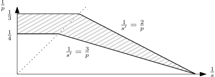
?figurename? 6: Region on which (1.10) is valid

We give some hints why (1.10) holds true and why the inverse inequality (with $\delta$-loss) seems a reasonable conjecture. Let $d\nu_{T}$ denote the “Lebesgue measure” on $P_{T}$. Then by Lemma 1.6

$$|\widehat{d\nu_{T}}(x_{1},x_{2},t)|\gtrsim t^{-\frac{1}{2}}\int_{0}^{T}e^{i(x_{2}\xi_{2}+t[\xi_{2}^{2}+\mathcal{O}(T^{-1}\xi_{2}^{3})])}d\xi_{2}$$

$$= Tt^{-\frac{1}{2}}\int_{0}^{1}e^{i(x_{2}T\eta+tT^{2}[\eta^{2}+\mathcal{O}(\eta^{3})])}d\eta\gtrsim t^{-1},$$

provided $x_{1}\ll t$ and $x_{2}\ll Tt$ (we may arrange matters in the preceding reductions so that the error term $\mathcal{O}(\eta^{3})$ is small compared to $\eta^{2}$). Hence, since we assume that $p>3,$

$$\|\widehat{d\nu_{T}}\|_{L^{p}(\mathbbm{R}^{3})}\gtrsim T^{\frac{1}{p}}.$$

Obviously $\|1\|_{L^{s}(P_{T},d\nu_{T})}=T^{\frac{1}{s}}$, so we see that

$$\|R^{*}_{T}\|_{L^{s}(P_{T})\to L^{p}(\mathbbm{R}^{3})}\gtrsim T^{\left(\frac{1}{p}-\frac{1}{s}\right)}.$$

Restricting $P_{T}$ to the region where $\xi_{2}\leq 1$, we see that also $\|R^{*}_{T}\|_{L^{s}(P_{T})\to L^{p}(\mathbbm{R}^{3})}\gtrsim 1,$ and combining these two lower bounds gives (1.10).

On the other hand, from Remark 4, (2.4) in [FU09] we easily obtain by an obvious rescaling-argument that for $1/{s^{\prime}}=3/p$ and $p>4$ (hence $1/p<1/s$), we have

$$\|R^{*}_{T}\|_{L^{s}(P_{T},d\nu_{T})\to L^{p}(\mathbbm{R}^{3})}\leq C,$$

uniformly in $T.$ It is conjectured that for the entire paraboloid $\mathcal{P}=\{(\xi_{1},\xi_{2},\xi_{1}^{2}+\xi_{2}^{2}):(\xi_{1},\xi_{2})\in\mathbbm{R}^{2}\},$ the adjoint restriction operator $R^{*}_{\mathcal{P},\mathbbm{R}^{2}}$ is bounded for $1/{s^{\prime}}=2/p$ and $p>3$ (hence $1/p<1/s$). It would be reasonable to expect the same kind of behaviour for suitable perturbations of the paraboloid, and subsets of those, such as $P_{T}$ (maybe with an extra factor $T^{\delta},$ for any $\delta>0$). By complex interpolation, the previous estimate in combination with the latter conjectural estimate would lead to

$$\|R^{*}_{T}\|_{L^{s}(P_{T},d\nu_{T})\to L^{p}(\mathbbm{R}^{3})}\leq C_{\delta}T^{\delta},$$

for every $\delta>0,$ provided that $1/p<1/s$ and $2/p<1/{s^{\prime}}<3/p.$ In combination with a trivial application of Hölder’s inequality this leads to the conjecture (1.11)

$$\|R^{*}_{T}\|_{L^{s}(P_{T})\to L^{p}(\mathbbm{R}^{3})}\leq C_{\delta}T^{\delta+\left(\frac{1}{p}-\frac{1}{s}\right)_{+}},$$

for every $\delta>0,$ provided $(1/s,1/p)$ lies within the shaded region in Figure 6.

1.4 The strategy of the approach

We will study certain bilinear operators. For a suitable pair of subsurfaces $S_{1},S_{2}\subset S$ (we will be more specific on this point later), we seek to establish bilinear estimates

$$\|R_{\mathbbm{R}^{2}}^{*}f_{1}R_{\mathbbm{R}^{2}}^{*}f_{2}\|_{L^{p}(\mathbbm{R}^{3})}\leq C_{p}C(S_{1},S_{2})\,\|f_{1}\|_{L^{2}(S_{1})}\|f_{2}\|_{L^{2}(S_{2})},$$

for functions $f_{1},\,f_{2}$ supported in $S_{1}$ and $S_{2},$ respectively.

For hypersurfaces with nonvanishing Gaussian curvature and principal curvatures of the same sign, the sharp estimates of this type, under the appropriate transversality assumption, appeared in [T03a] (after previous partial results in [TVV98], [TVI00]). For the light cone in any dimension, the analogous results were established in [W01], [T01a] (improving on earlier results in [Bo95b] and [TVI00]). For the case of principal curvatures of different sign, or with a smaller number of non-vanishing principal curvatures, sharp bilinear results are also known [L05], [V05], [LV10].

What is crucial for us is to know how the constant $C(S_{1},S_{2})$ explicitly depends on the pair of surfaces $S_{1}$ and $S_{2},$ in order to be able to sum all the bilinear estimates that we obtain for pairs of pieces of our given surface, to pass to a linear estimate. Classically, this is done by proving a bilinear estimate for one "generic" class of subsurfaces. For instance, if $S$ is the paraboloid, then other pairs of subsurfaces can be reduced to it by means suitable affine transformations and homogeneous rescalings. However, general surfaces do not come with such kind of self-similarity under these transformations, and it is one of the new features of this article that we will establish very precise bilinear estimates.

The bounds on the constant $C(S_{1},S_{2})$ that we establish will depend on the size of the domains and local principal curvatures of the subsurfaces, and we shall have to keep track of these during the whole proof. In this sense, many of the lemmas are generalized, quantitative versions of well known results from classical bilinear theory.

The pairs of subsurfaces that we would like to discuss are pieces of the surface sitting over two dyadic rectangles and satisfying certain separation or "transversality" assumptions. However, such a rectangle might touch one of the axis, where some principle curvature is vanishing. In this case we will decompose dyadically a second time. But even on these smaller sets, we do not have the correct "transversality" conditions; we first have to find a proper rescaling such that the scaled subsurfaces allow to run the bilinear machinery.

The following section will begin with the bilinear argument to provide us with a very general bilinear result for sufficiently "good" pairs of surfaces. In the subsequent section, we construct a suitable scaling in order to apply this general result to our situation. After rescaling and several additional arguments, we pass to a global bilinear estimate and finally proceed to the linear estimate.

A few more remarks on the notion will be useful: as mentioned before, it is very important to know precisely how the constants depend on the specific choice of subsurfaces. Moreover, there will appear other constants, depending possibly on $m_{1},m_{2},p,q$, or other quantities, but not explicitly on the choice of subsurfaces. We will not keep track of such types of constants, since it would even set a false focus and distract the reader. Instead we will simply use the symbol $\lesssim$ for an inequality involving one of these constants of minor importance. To be more precise on this, later we introduce a family of pairs of subsurfaces $\mathcal{S}_{0}$. Then for quantities $A,B:\mathcal{S}_{0}\to\mathbbm{R}$ the inequality $A\lesssim B$ means there exists a constant $C>0$ such that $A(S_{1},S_{2})\leq CB(S_{1},S_{2})$ uniformly for all $(S_{1},S_{2})\in\mathcal{S}_{0}$.

Moreover, we will also use the notation $A\sim B$ if $A\lesssim B$ and $B\lesssim A$. We will even use this notation for vectors, meaning their entries are comparable in each coordinate. Similarly, we write $A\ll B$ if there exists a constant $c>0$ such that $A(S_{1},S_{2})\leq cB(S_{1},S_{2})$ for all $(S_{1},S_{2})\in\mathcal{S}_{0}$ and $c$ is "small enough" for our purposes. This notion of being "sufficiently small" will in general depend on the situation and further constants, but the choice will be uniform in the sense that it will work for all pairs of subsurfaces in the class $\mathcal{S}_{0}$.

The inner product of two vectors $x,y$ will usually be denoted by $xy$ or $x\cdot y,$ occasionally also by $\langle x,y\rangle.$

2 General bilinear theory

2.1 Wave packet decomposition

We begin with what is basically a well known result, although we need a more quantitative version (cf. [T03b], [L05]).

Lemma 2.1.

Let $U\subset\mathbbm{R}^{d}$ be an open and bounded subset, and let $\phi\in C^{\infty}(U,\mathbbm{R}).$ We assume that there exist constants $\kappa>0$ and $D\leq{1}/{\kappa}$ such that $\|\partial^{\alpha}\phi\|_{\infty}\leq A_{\alpha}\kappa D^{2-|\alpha|}$ for all $\alpha\in\mathbbm{N}^{d}$ with $|\alpha|\geq 2$. Then for every $R\geq 1$ there exists a wave packet decomposition adapted to $\phi$ with tubes of radius $R/D=R^{\prime}$ and length $R^{2}/(D^{2}\kappa)=R^{\prime 2}/\kappa$, where we have put $R=R^{\prime}D.$

More precisely, consider the index sets $\mathcal{Y}=R^{\prime}\mathbbm{Z}^{d}$ and $\mathcal{V}=R^{\prime-1}\mathbbm{Z}^{d}\cap U$, and define for $w=(y,v)\in\mathcal{Y}\times\mathcal{V}=\mathcal{W}$ the tube

$$T_{w}=\Big{\{}(x,t)\in\mathbbm{R}^{d}\times\mathbbm{R}:|t|\leq\frac{R^{\prime 2}}{\kappa},\leavevmode\nobreak\ |x-y+t\nabla\phi(v)|\leq R^{\prime}\Big{\}}.$$ (2.1)

Then, given any function $f\in L^{2}(U),$ there exist functions (wave packets) $\{p_{w}\}_{w\in\mathcal{W}}$ and coefficients $c_{w}\in\mathbbm{C}$ such that $R^{*}_{\mathbbm{R}^{d}}f$ can be decomposed as

$$R^{*}_{\mathbbm{R}^{d}}f(x,t)=\sum\limits_{w\in\mathcal{W}}c_{w}p_{w}(x,t)$$

for every $t\in\mathbbm{R}$ with $|t|\leq{R^{\prime 2}}/{\kappa},$ in such a way that the following hold true:

1. $p_{w}=R^{*}_{\mathbbm{R}^{d}}(\textfrak{F}_{\mathbbm{R}^{d}}^{-1}(p_{w}(\cdot,0))).$

2. $\text{\rm supp\,}\textfrak{F}_{\mathbbm{R}^{d+1}}p_{w}\subset B((v,\phi(v)),2/R^{\prime}).$

3. $p_{w}$ is essentially supported in $T_{w},$ i.e., $|p_{w}(x,t)|\leq C_{N}R^{\prime-\frac{d}{2}}\left(1+\frac{|x-y+t\nabla\phi(v)|}{R^{\prime}}\right)^{-N}$ for every $N\in\mathbbm{N}.$ In particular, $\|p_{w}(\cdot,t)\|_{2}\lesssim 1$.

4. For all $W\subset\mathcal{W}$, we have $\|\sum\limits_{w\in W}p_{w}(\cdot,t)\|_{2}\lesssim|W|^{\frac{1}{2}}$.

5. $\|c\|_{\ell^{2}}\lesssim\|f\|_{L^{2}}$.

Moreover, the constants arising explicitly (such as the $C_{N}$) or implicitly in these estimates can be chosen to depend only on the constants $A_{\alpha}$ but no further on the function $\phi,$ and also not on the other quantities $R,D$ and $\kappa$ (such constants will be called admissible).

?figurename? 7: The tubes $T_{w}$ fill a horizontal strip

Remarks 2.2.

(i) Notice that no bound is required on $\nabla\phi$ at this stage; however, such bounds will become important later (for instance in (iii)).

(ii) Denote by $N(v)$ the normal vector at $(v,\phi(v))$ to the graph of $\phi$ which is given by $N(v)=(-\nabla\phi(v),1)$. Since $R^{\prime 2}/\kappa\geq R^{\prime},$ we may thus re-write

$$T_{w}=(y,0)+\Big{\{}tN(v):|t|\leq\frac{R^{\prime 2}}{\kappa}\Big{\}}+\mathcal{O}(R^{\prime}).$$

Moreover,

$$|x-y+t\nabla\phi(v)|=|(x,t)-(y,0)-tN(v)|\geq\text{\rm dist\,}((x,t),T_{w}).$$

It is then easily seen that (P3) can be re-written as

$$|p_{w}(z)|\leq C_{N}R^{\prime-\frac{d}{2}}\left(1+\frac{\text{\rm dist\,}(z,T_{w})}{R^{\prime}}\right)^{-N}$$

for all $z\in\mathbbm{R}^{d+1}$ with $|\langle z,e_{d+1}\rangle|\leq R^{\prime 2}/\kappa,$ where $e_{d+1}$ denotes the last vector of the canonical basis of $\mathbbm{R}^{d+1}.$ This justifies the statement that “$p_{w}$ is essentially supported in $T_{w}$.”

(iii) Notice further that we can re-parametrize the wave packets by lifting $\mathcal{V}$ to $\tilde{\mathcal{V}}=\{(v,\phi(v)):v\in\mathcal{V}\}\subset S$. If we now assume that $\|\nabla\phi\|\lesssim 1$, then we have $|(v,\phi(v))-(v^{\prime},\phi(v^{\prime}))|\sim|v-v^{\prime}|$, and thus $\tilde{\mathcal{V}}$ becomes an $R^{\prime-1}$-net in $S$. Finally, we shall identify a parameter $y\in\mathbbm{R}^{d}$ with the point $(y,0)$ in the hyperplane $\mathbbm{R}^{d}\times\{0\}$.

Proof:.

We will basically follow the proof by Lee [L05]; the only new feature consists in elaborating the precise role of the constant $\kappa$.
Let $\psi,\hat{\eta}\in C_{0}^{\infty}(B(0,1))$ be chosen in a such a way that for $\eta_{y}(x)=\eta(\frac{x-y}{R^{\prime}})$, $\psi_{v}(\xi)=\psi(R^{\prime}(\xi-v))$ we have $\sum\limits_{v\in\mathcal{V}}\psi_{v}=1$ on $U$ and $\sum\limits_{y\in\mathcal{Y}}\eta_{y}=1$. We also chose a slightly bigger function $\tilde{\psi}\in C_{0}^{\infty}(B(0,3))$ such that $\tilde{\psi}=1$ on $B(0,2)\supset\text{\rm supp\,}\psi+\text{\rm supp\,}\hat{\eta},$ and put $\tilde{\psi}_{v}(\xi)=\tilde{\psi}(R^{\prime}(\xi-v))$. Then the functions

$$F_{(y,v)}=\textfrak{F}_{\mathbbm{R}^{d}}^{-1}(\widehat{\psi_{v}f}\eta_{y})=(\psi_{v}f)\ast\check{\eta}_{y},\quad y\in\mathcal{Y},v\in\mathcal{V},$$

are essentially well-localized in both position and momentum/frequency space. Define $q_{w}=R_{\mathbbm{R}^{d}}^{*}(F_{w})$, $w=(y,v)\in\mathcal{W}$; up to a certain factor $c_{w},$ which will be determined later, these are already the announced wave packets, i.e., $q_{w}=c_{w}p_{w}$.
Since $f=\sum\limits_{w\in W}F_{w}$, we then have the decomposition $R_{\mathbbm{R}^{d}}^{*}f=\sum\limits_{w\in W}q_{w}.$ Let us concentrate on property (P3) - the other properties are then rather easy to establish. Since $\text{\rm supp\,}F_{(y,v)}\subset B(v,2/R^{\prime})$, we have for every $w=(y,v)\in\mathcal{W}$

$$q_{w}(x,t)= \int e^{-i(x\xi+t\phi(\xi))}F_{w}(\xi)\,d\xi=\int e^{-i(x\xi+t\phi(\xi))}F_{w}(\xi)\tilde{\psi}_{v}(\xi)\,d\xi$$

$$= (2\pi)^{-d}\iint e^{-i\big{(}(x-z)\xi+t\phi(\xi)\big{)}}\tilde{\psi}_{v}(\xi)\,d\xi\,\widehat{F_{w}}(z)\,dz$$

$$= (2\pi)^{-d}R^{\prime-d}\iint e^{-i\big{(}(x-z)(\frac{\xi}{R^{\prime}}+v)+t\phi(\frac{\xi}{R^{\prime}}+v)\big{)}}\tilde{\psi}(\xi)\,d\xi\,\widehat{F_{w}}(z)\,dz$$

$$= (2\pi)^{-d}R^{\prime-d}\int K(x-z,t)\widehat{F_{w}}(z)\,dz,$$

with the kernel

$$K(x,t)=\int e^{i\big{(}x(\frac{\xi}{R^{\prime}}+v)+t\phi(\frac{\xi}{R^{\prime}}+v)\big{)}}\tilde{\psi}(\xi)\,d\xi.$$

We claim that

$$|K(x,t)|\lesssim\left(1+\frac{|x+t\nabla\phi(v)|}{R^{\prime}}\right)^{-N}$$ (2.2)

for every $N\in\mathbbm{N}$. To this end, we shall estimate the oscillatory integral

$$K_{\lambda}=\int e^{i\lambda\Phi(\xi)}\tilde{\psi}(\xi)\,d\xi,$$

with phase

$$\Phi(\xi)=\frac{x(\frac{\xi}{R^{\prime}}+v)+t\phi(\frac{\xi}{R^{\prime}}+v)}{1+R^{\prime-1}|x+t\nabla\phi(v)|},$$

where we have put $\lambda=1+R^{\prime-1}|x+t\nabla\phi(v)|$. In order to prove (2.2), we may assume that $|x+t\nabla\phi(v)|\gg R^{\prime}$. Then integrations by parts will lead to $|K_{\lambda}|\lesssim\lambda^{-N}$ for all $N\in\mathbbm{N},$ hence to (2.2), provided we can show that

$$|\nabla\Phi(\xi)|\sim 1,\qquad\text{for all }\xi,$$ (2.3)

$$\text{and}\quad\|\partial^{\alpha}\Phi\|_{\infty}\lesssim 1\quad\text{for all }\alpha\geq 2,$$ (2.4)

and that the constants in these estimates are admissible. But,

$$\frac{|t||\nabla\phi(\frac{\xi}{R^{\prime}}+v)-\nabla\phi(v)|}{|x+t\nabla\phi(v)|}\ll \frac{|t||\nabla\phi(\frac{\xi}{R^{\prime}}+v)-\nabla\phi(v)|}{R^{\prime}}\lesssim\frac{|t|}{R^{\prime 2}}\|\phi^{\prime\prime}\|_{\infty}$$

$$\leq \frac{1}{\kappa}\|\phi^{\prime\prime}\|_{\infty}\leq 1,$$

for every $\xi\in\text{\rm supp\,}\tilde{\psi}$, hence

$$|t||\nabla\phi(\frac{\xi}{R^{\prime}}+v)-\nabla\phi(v)|\ll|x+t\nabla\phi(v)|.$$

Thus

$$|\nabla\Phi(\xi)|=\frac{|x+t\nabla\phi(\frac{\xi}{R^{\prime}}+v)|}{R^{\prime}+|x+t\nabla\phi(v)|}= \frac{|x+t\nabla\phi(v)-t[\nabla\phi(v)-\nabla\phi(\frac{\xi}{R^{\prime}}+v)]|}{R^{\prime}+|x+t\nabla\phi(v)|}$$

$$\sim \frac{|x+t\nabla\phi(v)|}{R^{\prime}+|x+t\nabla\phi(v)|}\sim 1,$$

which verifies (2.3). And, for $|\alpha|\geq 2$ we have

$$|\partial^{\alpha}\Phi(\xi)|\leq |tR^{\prime-|\alpha|}(\partial^{\alpha}\phi)(\frac{\xi}{R^{\prime}}+v)|\overset{}{\lesssim}\frac{R^{\prime 2}}{\kappa}R^{\prime-|\alpha|}\kappa D^{2-|\alpha|}\leq(DR^{\prime})^{2-|\alpha|}=R^{2-|\alpha|}\leq 1,$$

which gives (2.4). It is easily checked that the constants in these estimates can be chosen to be admissible. Following the proof in [L05], we conclude that

$$|q_{w}(x,t)|\lesssim R^{\prime-d}\int\left|K(x-z-y,t)\widehat{F_{w}}(z+y)\right|dz$$

$$= R^{\prime-d}\int\left|K(x-z-y,t)\eta\left(\frac{z}{R^{\prime}}\right)\widehat{\psi_{v}f}(z+y)\right|dz$$

$$\lesssim \left(1+\frac{|x-y+t\nabla\phi(v)|}{R^{\prime}}\right)^{-N}\mathop{M}(\widehat{\psi_{v}f})(y),$$

where $M$ denotes the Hardy-Littlewood maximal operator. Thus, by choosing $c_{w}=c_{(y,v)}={R^{\prime}}^{\frac{d}{2}}M(\widehat{\psi_{v}f})(y),$ we obtain (P3).

Properties (P1) and (P2) follow from the definition of the wave packets. From (P2) and (P3) we can deduce (P4). For (P5), we refer to [L05]. $\Box$

In view of our previous remarks, it is easy to re-state Lemma 2.1 in a more coordinate-free way. For any given hyperplane $H=n^{\perp}\subset\mathbbm{R}^{d+1}$, with $n$ a unit vector (so that $\mathbbm{R}^{d+1}=H+\mathbbm{R}n$), define the partial Fourier (co)-transform

$$\textfrak{F}_{H}^{-1}f(\xi+tn)=\int_{H}f(x+tn)e^{ix\cdot\xi}\,dx,\quad\xi\in H,t\in\mathbbm{R}.$$

Moreover, if $U\subset H$ is open and bounded, and if $\phi_{H}\in C^{\infty}(U,\mathbbm{R})$ is given, then consider the smooth hypersurface $S=\{\eta+\phi_{H}(\eta)n:\eta\in U\}\subset\mathbbm{R}^{d+1},$ and define the corresponding Fourier extension operator

$$R^{*}_{H}f(x+tn)=\int_{U}f(\eta)e^{-i(x\eta+t\phi_{H}(\eta))}\,d\eta=\int_{U}f(\eta)e^{-i<x+tn,\eta+\phi_{H}(\eta)n>}\,d\eta,$$

for $(x,t)\in H\times\mathbbm{R},f\in L^{2}(U).$ Notice that $R^{*}_{\mathbbm{R}^{d}}$ corresponds to the special case $H=\mathbbm{R}^{d}\times\{0\},$ and thus by means of a suitable rotation, mapping $e_{d+1}$ to $n,$ we immediately obtain the following

Corollary 2.3 (Wave packet decomposition).

Let $U\subset H$ be an open and bounded subset, and let $\phi_{H}\in C^{\infty}(U,\mathbbm{R}).$ We assume that there are constants $\kappa>0$ and $D\leq{1}/{\kappa}$ such that $\|\phi_{H}^{(l)}\|_{\infty}\leq A_{l}\kappa D^{2-l}$ for every $l\in\mathbbm{N}$ with $l\geq 2,$ where $\phi_{H}^{(l)}$ denotes the total derivative of $\phi_{H}$ of order $l,$ and in addition that $\|\phi^{\prime}\|_{\infty}\leq A.$ Then for every $R\geq 1$ there exists a wave packet decomposition adapted to $S$ and the decomposition of $\mathbbm{R}^{d+1}$ into $\mathbbm{R}^{d+1}=H+\mathbbm{R}n,$ with tubes of radius $R/D=R^{\prime}$ and length $R^{2}/(D^{2}\kappa)=R^{\prime 2}/\kappa,$ where $R=R^{\prime}D.$

More precisely, there exists an $R^{\prime}$-lattice $\mathcal{Y}$ in $H$ and an $R^{\prime-1}$-net $\mathcal{V}$ in $S$ such that the following hold true: if we denote by $\mathcal{W}$ the index set $\mathcal{W}=\mathcal{Y}\times\mathcal{V}$ and associate to $w=(y,v)\in\mathcal{Y}\times\mathcal{V}=\mathcal{W}$ the tube-like set

$$T_{w}=y+\Big{\{}tN(v):|t|\leq\frac{R^{\prime 2}}{\kappa}\Big{\}}+B(0,R^{\prime}),$$ (2.5)

then for every given function $f\in L^{2}(U)$ there exist functions (wave packets) $\{p_{w}\}_{w\in\mathcal{W}}$ and coefficients $c_{w}\in\mathbbm{C}$ such that for every $x=x^{\prime}+tn\in\mathbbm{R}^{d+1}$ with $|t|\leq\frac{R^{\prime 2}}{\kappa}$ and $x^{\prime}\in H,$ we may decompose $R_{H}^{*}f(x)$ as

$$R_{H}^{*}f(x)=\sum\limits_{w\in\mathcal{W}}c_{w}p_{w}(x),$$

in such a way that the following hold true:

1. $p_{w}=R_{H}^{*}(\textfrak{F}_{H}^{-1}(p_{w}|_{H}))$,

2. $\text{\rm supp\,}\textfrak{F}_{\mathbbm{R}^{d+1}}p_{w}\subset B(v,R^{\prime-1})$ and $\text{\rm supp\,}\textfrak{F}_{H}(p_{w}(\cdot+tn))\subset B(v^{\prime},\mathcal{O}(R^{\prime-1}))$, where $v^{\prime}$ denotes the orthogonal projection of $v\in S$ to $H$.

3. $p_{w}$ is essentially supported in $T_{w}$, i.e., $|p_{w}(x)|\leq C_{N}R^{\prime-1}\left(1+\frac{\text{\rm dist\,}(x,T_{w})}{R^{\prime}}\right)^{-N}$.

4. For all $W\subset\mathcal{W}$, we have $\|\sum\limits_{w\in W}p_{w}(\cdot+tn)\|_{L^{2}(H)}\lesssim|W|^{\frac{1}{2}}$.

5. $\|c\|_{\ell^{2}}\lesssim\|f\|_{L^{2}}$.

Moreover, the constants arising in these estimates can be chosen to depend only on the constants $A_{l}$ and $A,$ but no further on the function $\phi_{H},$ and also not on the other quantities $R,D$ and $\kappa$ (such constants will be called admissible).

Notice that, unlike as in Lemma 2.1, we may here choose an $R^{\prime-1}$-net in $S$ in place of an $R^{\prime}$ -lattice in $H$ for the parameter set $\mathcal{V},$ because of our assumed bound on $\phi_{H}^{\prime}.$

It will become important that under suitable additional assumptions on the position of a given hyperplane $H$, we may re-parametrize a given smooth hypersurface $S=\{(\xi,\phi(\xi)):\xi\in U\}$ (where $U$ is an open subset of $\mathbbm{R}^{d}$) also in the form

$$S=\{\eta+\phi_{H}(\eta)n:\eta\in U_{H}\},$$

where $U_{H}$ is an open subset of $H$ and $\phi_{H}\in C^{\infty}(U_{H},\mathbbm{R}).$

Lemma 2.4 (Re-parametrization).

Let $H_{1}=n_{1}^{\perp}$ and $H_{2}=n_{2}^{\perp}$ be two hyperplanes in $\mathbbm{R}^{d+1},$ where $n_{1}$ and $n_{2}$ are given unit vectors. Let $K=H_{1}\cap H_{2},$ and choose unit vectors $h_{1},h_{2}$ orthogonal to $K$ such that $H_{1}=K+\mathbbm{R}h_{1},\quad H_{2}=K+\mathbbm{R}h_{2}.$ Let $U_{1}\subset H_{1}$ be an open bounded subset such that for every $x^{\prime}\in K,$ the section $U_{1}^{x^{\prime}}=\{u\in\mathbbm{R}:x^{\prime}+uh_{1}\subset U_{1}\}$ is an (open) interval, and let $\phi_{1}\in C^{\infty}(U_{1},\mathbbm{R})$ satisfying the assumptions of Corollary 2.3. Setting $B=\kappa D^{2}$ and $r=D^{-1},$ an equivalent way to state this is that there are constants $B,r>0$ such that $Br\leq 1$, $\|\phi_{1}^{\prime}\|_{\infty}\leq A$ and $\|\phi_{1}^{(l)}\|_{\infty}\leq A_{l}Br^{l}$ for every $l\in\mathbbm{N}$ with $l\geq 2.$ Denote by $S$ the hypersurface

$$S=\{\eta+\phi_{1}(\eta)n_{1}:\eta\in U_{1}\}\subset\mathbbm{R}^{d+1},$$

and again by $v\mapsto N(v)$ the corresponding unit normal field on $S.$

Assume furthermore that the vector $n_{2}$ is transversal to $S,$ i.e., $|\langle n_{2},N(v)\rangle|\geq a>0$ for all $v\in S.$ Then there exist an open bounded subset $U_{2}\subset H_{2}$ such that for every $x^{\prime}\in K,$ the section $U_{2}^{x^{\prime}}=\{s\in\mathbbm{R}:x^{\prime}+sh_{2}\in U_{2}\}$ is an interval, and a function $\phi_{2}\in C^{\infty}(U_{2},\mathbbm{R})$ so that we may re-write

$$S=\{\xi+\phi_{2}(\xi)n_{2}:\xi\in U_{2}\}.$$ (2.6)

Moreover, the derivatives of $\phi_{2}$ satisfy estimates of the same form as those of $\phi_{1},$ up to multiplicative constants which are admissible, i.e., which depend only on the constants $A_{l},A$ and $a.$

Finally, given any $f_{1}\in L^{2}(U_{1}),$ there exists a unique function $f_{2}\in L^{2}(U_{2})$ such that

$$R^{*}_{H_{1}}f_{1}=R^{*}_{H_{2}}f_{2},$$ (2.7)

and $\|f_{1}\|_{2}\sim\|f_{2}\|_{2},$ where the constants in these estimates are admissible.

Proof:.

Assume that (2.6) holds true. Then, given any point $\eta+\phi_{H}(\eta)n_{1}\in S,$ with $\eta=x^{\prime}+uh_{1}\in U_{1},x^{\prime}\in K,$ we find some $\xi=x^{\prime}+sh_{2}\in U_{2}$ such that

$$x^{\prime}+uh_{1}+\phi_{1}(x^{\prime}+uh_{1})n_{1}=x^{\prime}+sh_{2}+\phi_{2}(x^{\prime}+sh_{2})n_{2},$$ (2.8)

which shows that necessarily

$$s=\langle uh_{1}+x^{\prime}+\phi_{1}(x^{\prime}+uh_{1})n_{1},h_{2}\rangle.$$ (2.9)

Let us therefore define the mapping $G:U_{1}\to H_{2}$ by

$$G(x^{\prime}+uh_{1})=x^{\prime}+\langle uh_{1}+x^{\prime}+\phi_{1}(x^{\prime}+uh_{1})n_{1},h_{2}\rangle h_{2}.$$

Moreover, fixing an orthonormal basis $E_{1},\dots,E_{d-1}$ of $K$ and extending this by the vector $h_{1}$ respectively $h_{2}$ in order to obtain bases of $H_{1}$ and $H_{2}$ and working in the corresponding coordinates, we may assume without loss of generality that $U_{1}$ is an open subset of $\mathbbm{R}^{d-1}\times\mathbbm{R},$ since $\dim K=d-1,$ and that $G$ is a mapping $G:U_{1}\to\mathbbm{R}^{d-1}\times\mathbbm{R},$ given by

$$G(x^{\prime},u)=(x^{\prime},g(x^{\prime},u)),$$

where

$$g(x^{\prime},u)=\langle x^{\prime}+uh_{1}+\phi_{1}(x^{\prime},u)n_{1},h_{2}\rangle.$$

To show that $G$ is a diffeomorphism onto its image $U_{2}=G(U_{1}),$ observe that

$${\partial}_{u}G(x^{\prime},u)=(0,{\partial}_{u}g(x^{\prime},u))=(0,\langle h_{1}+{\partial}_{u}\phi_{1}(x^{\prime},u)n_{1},h_{2}\rangle).$$

On the other hand, the vector

$$N_{0}=-{\partial}_{u}\phi_{1}(x^{\prime},u)h_{1}-\sum_{j=1}^{k}{\partial}_{x_{j}}\phi(x^{\prime},u)E_{j}+n_{1}$$

is normal to $S$ at the point $x^{\prime}+uh_{1}+\phi_{1}(x^{\prime}+uh_{1})n_{1}$ (here $x^{\prime}=\sum_{j=1}^{d-1}x_{j}E_{j}$), and $|N_{0}|\sim 1.$ Thus, our transversality assumption implies that

$$|\langle-{\partial}_{u}\phi_{1}(x^{\prime},u)h_{1}+n_{1},n_{2}\rangle|\gtrsim a>0.$$ (2.10)

But, $\{h_{j},n_{j}\}$ forms an orthonormal basis of $K^{\perp}$ for $j=1,2,$ and thus, rotating all these vectors by an angle of $\pi/2,$ we see that (2.10) is equivalent to $|\langle{\partial}_{u}\phi_{1}(x^{\prime},u)n_{1}+h_{1},h_{2}\rangle|\gtrsim a>0,$ so that

$$|{\partial}_{u}g(x^{\prime},u)|\gtrsim a>0.$$

Given the special form of $G,$ this also implies that

$$|\det G^{\prime}(x^{\prime},u)|=|{\partial}_{u}g(x^{\prime},u)|\gtrsim a>0.$$

Consequently, for $x^{\prime}$ fixed, the mapping $u\mapsto g(x^{\prime}.u)$ is a diffeomorphism from the interval $U_{1}^{x^{\prime}}$ onto an open interval $U_{2}^{x^{\prime}},$ and thus $G$ is bijective onto its image $U_{2},$ in fact even a diffeomorphism, and $U_{2}$ fibers into the intervals $U_{2}^{x^{\prime}}.$ Indeed, the inverse mapping $F=G^{-1}:U_{2}\to U_{1}$ of $G$ is also of the form

$$F(x^{\prime},s)=(x^{\prime},f(x^{\prime},s)),$$

where

$$g(x^{\prime},f(x^{\prime},s)=s.$$ (2.11)

In combination with (2.8) this shows that (2.6) holds indeed true, with

$$\phi_{2}(x^{\prime},s)=f(x^{\prime},s)\langle h_{1},n_{2}\rangle+\phi_{1}(F(x^{\prime},s))\langle n_{1},n_{2}\rangle.$$ (2.12)

Moreover, if $f_{1}\in L^{2}(U_{1}),$ then, by (2.8) and a change of coordinates,

$$R^{*}_{H_{1}}f_{1}(y)=\iint_{U_{1}}f_{1}(x^{\prime},u)e^{-i\langle y,x^{\prime}+uh_{1}+\phi_{1}(x^{\prime},u)n_{1}\rangle}\,dx^{\prime}du$$

$$=\iint_{U_{2}}f_{1}(F(x^{\prime},s))|\det F^{\prime}(x^{\prime},s)|\,e^{-i\langle y,x^{\prime}+sh_{2}+\phi_{2}(x^{\prime},s)n_{2}\rangle}\,dx^{\prime}ds,$$

so that (2.7) holds true, with

$$f_{2}(x^{\prime}+sh_{2})=f_{1}\big{(}x^{\prime}+f(x^{\prime},s)h_{1}\big{)}\,|\det F^{\prime}(x^{\prime},s)|.$$ (2.13)

Our estimates for derivatives of $F$ show that $|\det F^{\prime}(x^{\prime},s)|\sim 1,$ with admissible constants, so that in particular $\|f_{1}\|_{2}\sim\|f_{2}\|_{2}.$

What remains is the control of the derivatives of $\phi_{2}.$ This somewhat technical part of the proof will be based on Faà di Bruno’s theorem and is deferred to the Appendix (see Subsection 7.2). $\Box$

We shall from now on restrict ourselves to dimension $d=2.$ The following lemma will deal with the separation of tubes along certain types of curves, for a special class of 2-hypersurfaces. It will later be applied to intersection curves of two hypersurfaces.

Lemma 2.5 (Tube-separation along intersection curve).

Let $\mathcal{Y},\mathcal{V},\mathcal{W},R,T_{w}$ be as in Corollary 2.3. Moreover assume that $\phi\in C^{\infty}(U,\mathbbm{R})$, $U\subset\mathbbm{R}^{2},$ such that $\partial_{i}^{2}\phi(x)\sim\kappa_{i}$ for all $x\in U,i=1,2,$ and $\partial_{1}\partial_{2}\phi=0$. Define $\kappa=\kappa_{1}\vee\kappa_{2}$. Let $\gamma=(\gamma_{1},\gamma_{2})$ be a curve in $U$ with such that $|\dot{\gamma}_{i}|\sim 1$ for $i=1,2.$ Then for all pairs of points $v_{1},v_{2}\in{\rm im}(\gamma)+\mathcal{O}(R^{\prime-1})$ such that $v_{1}-v_{2}={j}/{R^{\prime}}$, where $j\in\mathbbm{Z}^{2}$ and $|j|\gg 1,$ the following separation condition holds true (again with constants in these estimates which are admissible in the obvious sense):

$$|\nabla\phi(v_{1})-\nabla\phi(v_{2})|\sim|j|\frac{R^{\prime}}{R^{\prime 2}/\kappa}.$$

Proof:.

Choose $t_{1},t_{2}$ such that $v_{i}=\gamma(t_{i})+\mathcal{O}(R^{\prime-1})$. Then

$$|\nabla\phi(v_{i})-\nabla\phi(\gamma(t_{i}))|\leq\|\phi^{\prime\prime}|_{U}\|_{\infty}|v_{i}-\gamma(t_{i})|\lesssim\frac{\kappa}{R^{\prime}}.$$ (2.14)

Therefore

$$\frac{|j|}{R^{\prime}}= |v_{1}-v_{2}|=|\gamma(t_{1})-\gamma(t_{2})|+\mathcal{O}(R^{\prime-1})\sim|\dot{\gamma}_{1}||t_{1}-t_{2}|+|\dot{\gamma}_{2}||t_{1}-t_{2}|+\mathcal{O}(R^{\prime-1})$$

$$\sim |t_{1}-t_{2}|+\mathcal{O}(R^{\prime-1}),$$

and since $|j|\gg 1$, we see that $|t_{1}-t_{2}|\sim{|j|}/{R^{\prime}}.$ By our assumptions on $\phi$ and (2.14), we thus see that there exist $s_{1}$ and $s_{2}$ lying between $t_{1}$ and $t_{2}$ such that

$$|\nabla\phi(v_{1})-\nabla\phi(v_{2})|\geq |\nabla\phi(\gamma(t_{1}))-\nabla\phi(\gamma(t_{2}))|-\kappa\mathcal{O}(R^{\prime-1})$$

$$\sim \big{(}|\partial_{1}^{2}\phi(\gamma(s_{1}))\dot{\gamma}(s_{1})|+|\partial_{2}^{2}\phi(\gamma(s_{2}))\dot{\gamma}(s_{2})|\big{)}\,|t_{1}-t_{2}|-\kappa\mathcal{O}(R^{\prime-1})$$

$$\sim (\kappa_{1}+\kappa_{2})\frac{|j|}{R^{\prime}}+\kappa\mathcal{O}(R^{\prime-1})$$

$$\sim |j|\frac{\kappa}{R^{\prime}},$$

where we used again that $|j|\gg 1$. $\Box$

2.2 A bilinear estimate for normalized hypersurfaces

In this section, we shall work under the following

General Assumptions: Let $\phi\in C^{\infty}(\mathbbm{R}^{2})$ such that $\partial_{1}\partial_{2}\phi\equiv 0$, and let

$$S_{j}=\{(\eta,\phi(\eta):\eta\in U_{j}\},\quad U_{j}=r^{(j)}+[0,d^{(j)}_{1}]\times[0,d^{(j)}_{2}],\qquad j=1,2,$$

where $r^{(j)}\in\mathbbm{R}^{2}$ and $d^{(j)}_{1},d^{(j)}_{2}>0.$ We assume that the principal curvature of $S_{j}$ in the direction of $\eta_{1}$ is comparable to $\kappa^{(j)}_{1}>0,$ and in the direction of $\eta_{2}$ to $\kappa^{(j)}_{2}>0,$ up to some fixed multiplicative constants. We then put for $j=1,2,$

$$\kappa^{(j)}=\kappa^{(j)}_{1}\vee\kappa^{(j)}_{2},\qquad\bar{\kappa}_{i}=\kappa^{(1)}_{i}\vee\kappa^{(2)}_{i}$$

$$\bar{\kappa}=\bar{\kappa}_{1}\vee\bar{\kappa}_{2}=\kappa^{(1)}\vee\kappa^{(2)}$$ (2.15)

$$\bar{d}_{i}=d_{i}^{(1)}\vee d^{(2)}_{i},\qquad D=\min\limits_{i,j}d_{i}^{(j)}.$$

The vector field $N=(-\nabla\phi,1)$ is normal to $S_{1}$ and $S_{2},$ and thus $N_{0}={N}/{|N|}$ is a unit normal field to these hypersurfaces. We make the following additional assumptions:

1. For all $i,j=1,2$ and all $\eta\in U_{j}$, we have

   $$|\partial_{i}\phi(\eta)-\partial_{i}\phi(r^{(j)})|\lesssim\kappa_{i}^{(j)}d_{i}^{(j)}\quad\mbox{and}\quad\bar{\kappa}_{i}\bar{d}_{i}\lesssim 1$$ (2.16)

   (notice that the first inequality follows already from our earlier assumptions).

2. For all $\eta\in U_{1}\cup U_{2}$ and for all $\alpha\in\mathbbm{N}^{2},|\alpha|\geq 2,$ we have $|\partial^{\alpha}\phi(\eta)|\lesssim\bar{\kappa}D^{2-|\alpha|}$.

3. For $i=1,2,$ i.e., with respect to both variables, the following separation condition holds true:

   $$|\partial_{i}\phi(\eta^{1})-\partial_{i}\phi(\eta^{2})|\sim 1\quad\mbox{for all }\eta^{j}\in U_{j},\ j=1,2.$$ (2.17)

The set of all pairs $(S_{1},S_{2})$ of hypersurfaces satisfying these properties will be denoted by $\mathcal{S}_{0}$ (note that it does depend on the constants hidden by the symbols $\lesssim$ and $\sim$).

The main goal of this chapter will be to establish a local, bilinear Fourier extension estimate on suitable cuboids adapted to the wave packets.

Theorem 2.6.

Assume that $5/{3}\leq p\leq 2.$ Let us choose $r\in\mathbbm{R}^{2}$ such that $r=r^{(j)},$ if $\kappa^{(j)}=\kappa^{(1)}\wedge\kappa^{(2)}.$ Then for every $\alpha>0$ there exist constants $C_{\alpha},\gamma_{\alpha}>0$ such that for every pair $S=(S_{1},S_{2})\in\mathcal{S}_{0}$, every parameter $R\geq 1$ and all functions $f_{j}\in L^{2}(S_{j})$, $j=1,2$ we have

$$\|R_{\mathbbm{R}^{2}}^{*}f_{1}\,R_{\mathbbm{R}^{2}}^{*}f_{2}\|_{L^{p}(Q^{0}_{S_{1},S_{2}}(R))}\leq C_{\alpha}R^{\alpha}(\kappa^{(1)}\kappa^{(2)})^{\frac{1}{2}-\frac{1}{p}}D^{3-\frac{5}{p}}\log^{\gamma_{\alpha}}(C_{0}(S))\,\|f_{1}\|_{2}\|f_{2}\|_{2},$$ (2.18)

where

$$Q^{0}_{S_{1},S_{2}}(R)=\left\{x\in\mathbbm{R}^{3}:\leavevmode\nobreak\ |x_{i}+\partial_{i}\phi(r)x_{3}|\leq\frac{R^{2}}{D^{2}\bar{\kappa}},i=1,2,\leavevmode\nobreak\ |x_{3}|\leq\frac{R^{2}}{D^{2}(\kappa^{(1)}\wedge\kappa^{(2)})}\right\},$$ (2.19)

with

$$C_{0}(S)=\frac{\bar{d}_{1}^{2}\bar{d}_{2}^{2}}{D^{4}}(D[\kappa^{(1)}\wedge\kappa^{(2)}])^{-\frac{1}{p}}(D\kappa^{(1)}D\kappa^{(2)})^{-\frac{1}{2}}.$$ (2.20)

Notice that $C_{0}(S)\gtrsim 1.$

Remark 2.7.

If $\kappa^{(1)}=\kappa^{(2)}=\bar{\kappa}$, then $r$ is not well defined. But in this case the two sets $Q^{0}_{S_{1},S_{2}}(R;j)=\{x\in\mathbbm{R}^{3}:\leavevmode\nobreak\ |x_{i}+\partial_{i}\phi(r^{(j)})x_{3}|\leq\frac{R^{2}}{D^{2}\bar{\kappa}},i=1,2,\leavevmode\nobreak\ |x_{3}|\leq\frac{R^{2}}{D^{2}\bar{\kappa}}\}$, $j=1,2$, essentially coincide. Indeed, since $|\nabla\phi(r^{(1)})-\nabla\phi(r^{(2)})|\sim 1$ (due to the transversality assumption (iii)), an easy geometric consideration shows that

$$aQ^{0}_{S_{1},S_{2}}(R;1)\subset Q^{0}_{S_{1},S_{2}}(R;2)\subset bQ^{0}_{S_{1},S_{2}}(R;1),$$

for some constants $a,b$ which do not depend on $R$ and the class $\mathcal{S}_{0}$ from which $S=(S_{1},S_{2})$ is taken.

By applying a suitable affine transformation whose linear part fixes the points of $\mathbbm{R}^{2}\times\{0\},$ if necessary, we may assume without loss of generality that $r=0$ and $\nabla\phi(r)=0$. Notice that conditions (i)-(iii) and the conclusion of the theorem are invariant under such affine transformations.

In fact, we we shall then prove estimate (2.18) in the theorem on the even larger cuboid

$$Q_{S_{1},S_{2}}(R)=\left\{x\in\mathbbm{R}^{3}:\leavevmode\nobreak\ |x_{i_{0}}|\leq\frac{R^{2}}{D^{2}\bar{\kappa}},\leavevmode\nobreak\ \|x\|_{\infty}\leq\frac{R^{2}}{D^{2}(\kappa^{(1)}\wedge\kappa^{(2)})}\right\},$$ (2.21)

for an appropriate choice of the coordinate direction $x_{i_{0}},i_{0}\in\{1,2\},$ in which the cuboid has smaller side length. Later we shall need to combine different cuboids which may possibly have their smaller side lengths in different directions. Then it will become necessary to restrict to their intersection, which leads to (2.19).

Indeed, we shall see that there will be two directions in which the side length of the cuboids are dictated by the length of the wave packets, and one remaining third direction for which we shall have more freedom in choosing the side length.

Observe also that $\bar{\kappa}_{i}\bar{d}_{i}\lesssim 1$, and thus we may even assume without loss of generality that

$$\bar{\kappa}_{i}\bar{d}_{i}\ll 1\quad\text{for all }i=1,2,$$ (2.22)

simply by decomposing $S_{1}$ and $S_{2}$ into a finite number of subsets for which the side lengths of corresponding rectangles $U_{j}$ are sufficiently small fractions of the given $d_{i}^{(j)}.$

For $\eta^{j}\in U_{j}$ define

$$\phi_{1}(\eta)=\phi(\eta-\eta^{2})+\phi(\eta^{2}),\qquad\eta\in\eta^{2}+U_{1}$$

$$\phi_{2}(\eta)=\phi(\eta-\eta^{1})+\phi(\eta^{1}),\qquad\eta\in\eta^{1}+U_{2}.$$

The set $((\eta^{2},\phi(\eta^{2}))+S_{1})\cap((\eta^{1},\phi(\eta^{1}))+S_{2})=\mathop{\rm graph}(\phi_{1})\cap\mathop{\rm graph}(\phi_{2})$ will be called an intersection curve of $S_{1}$ and $S_{2}$. It agrees with the graph of $\phi_{1}$ (or $\phi_{2}$) restricted to the set where $\psi=\phi_{1}-\phi_{2}=0$. On this set, the normal field $N_{j}(\eta)=(-\nabla\phi_{j}(\eta),1)$ forms the conical set

$$\Gamma_{j}=\{sN_{j}(\eta)|s\in\mathbbm{R},\psi(\eta)=0\}.$$

In the sequel, we shall use the abbreviation $j+1\!\!\!\mod 2=2,$ if $j=1,$ and $j+1\!\!\!\mod 2=1,$ if $j=2.$

Lemma 2.8.

Let $(S_{1},S_{2})\in\mathcal{S}_{0}$. Assume that $\nabla\phi(r)=0$ for some $r\in S_{1}\cup S_{2}$ and $\bar{\kappa}_{i}\bar{d}_{i}\ll 1$. Then the following hold true:

1. $D\kappa_{i}^{(j)}\ll 1$ for all $i,j=1,2$.

2. $|\nabla\phi(\eta)|\lesssim 1$ for all $(\eta,\phi(\eta))\in S_{1}\cup S_{2}$.

3. The unit normal fields on $S_{1}$ and $S_{2}$ are transversal, i.e.,

   $$|N_{0}(\eta^{1})-N_{0}(\eta^{2})|\sim 1\quad\text{for all }(\eta^{j},\phi(\eta^{j}))\in S_{j}.$$ (2.23)

4. $N_{j}$ and $\Gamma_{j+1\!\!\!\mod 2}$ are transversal for $j=1,2$ and for any choice of intersection curve of $S_{1}$ and $S_{2}$.

5. If $\gamma$ is a parametrization by arclength $t$ of the projection of an intersection curve of $S_{1}$ and $S_{2}$ to the first two coordinates $\eta\in\mathbbm{R}^{2},$ then $|\dot{\gamma}_{1}|\sim 1\sim|\dot{\gamma}_{2}|$.

Proof:.

We shall denote by $\eta=\tilde{x}\in\mathbbm{R}^{2}$ the projection of a point in $x\in\mathbbm{R}^{3}$ to its first two coordinates. (a) is clear since $D=\min\limits_{i,j=1,2}d_{i}^{(j)}$. To prove (b), notice that for any $x,x^{\prime}\in S_{1}\cup S_{2}$ we have $|\nabla\phi(\tilde{x})-\nabla\phi(\tilde{x}^{\prime})|\lesssim 1$: if $x$ and $x^{\prime}$ belong to different hypersurface $S_{j}$, we apply condition (iii) from the definition of $\mathcal{S}_{0}$, and if $x$ and $x^{\prime}$ are in the same hypersurface $S_{j}$, we use condition (a). Thus we have $|\nabla\phi(\tilde{x})|=|\nabla\phi(\tilde{x})-\nabla\phi(r)|\lesssim 1$ for all $x\in S_{1}\cup S_{2}$.
This gives $|N(\tilde{x})|=\sqrt{1+|\nabla\phi(\tilde{x})|^{2}}\sim 1$ for all $x\in S_{1}\cup S_{2},$ which already implies the transversality of the normal fields:

$$|N_{0}(\eta^{1})-N_{0}(\eta^{2})|\sim|N(\eta^{1})-N(\eta^{2})|=|\nabla\phi(\eta^{1})-\nabla\phi(\eta^{2})|\sim 1$$

for all $(\eta^{j},\phi(\eta^{j}))\in S_{j},\ j=1,2.$

We shall prove (e) first, since (e) will be needed for the proof of (d). It suffices to prove that $|\partial_{i}\psi(\eta)|\sim 1$ for all $\eta$ such that $\eta-\eta^{j}\in U_{j+1\!\!\!\mod 2}$, $\eta^{j}\in U_{j},$ since the tangent to the curve $\gamma$ at any point $\gamma(t)$ is orthogonal to $\nabla\psi(\gamma(t)).$ But, in view of (2.17),

$$|\partial_{i}\psi(\eta)|=|\partial_{i}\phi(\eta-\eta^{2})-\partial_{i}\phi(\eta-\eta^{1})|{\sim}1.$$

For the claim (d), since the claim is symmetric in $j\in\{1,2\},$ it suffices to show that $N_{1}$ and $\Gamma_{2}$ are transversal. Since we have

$$|N_{1}(\eta)-N_{1}(\eta^{\prime})|=|\nabla\phi_{1}(\eta)-\nabla\phi_{1}(\eta^{\prime})|\lesssim\kappa^{(1)}_{1}d^{(1)}_{1}+\kappa^{(1)}_{2}d^{(1)}_{2}\ll 1$$

for all $\eta,\eta^{\prime}\in U_{1}+\eta^{2}$, whereas $|N_{1}(\eta)|\sim 1$ for all $\eta\in U_{1}+\eta^{2}$, it is even enough to show that $N_{1}(\eta)$ and the tangent space $T_{N_{2}(\eta)}\Gamma_{2}$ of $\Gamma_{2}$ at the point $N_{2}(\eta)$ are transversal. Since $\gamma$ is a parametrization by arclength of the zero set of $\psi$, the tangent space of $\Gamma_{2}$ at the point $N_{2}(\eta)$ for $\eta=\gamma(t)$ is spanned by $N_{2}(\eta)$ and $(-D^{2}\phi_{2}(\eta)\;\dot{\gamma}(t),0)$, where $D^{2}\phi_{2}$ denotes the Hessian matrix of $\phi_{2}.$ But, recalling that we assume that $\partial_{1}\partial_{2}\phi\equiv 0,$ we see that the vectors $N_{2}(\eta)$ and $\frac{1}{\kappa^{(2)}}(-D^{2}\phi_{2}(\eta)\;\dot{\gamma}(t),0)$ form an “almost” orthonormal frame for the tangent space $T_{N_{2}(\eta)}\Gamma_{2},$ and thus the transversality can be checked by estimating the volume $V$ of the parallelepiped spanned by $N_{1}(\eta)$ and these two vectors, which is given by

$$V =\left|\begin{array}[]{ccc}-\partial_{1}\phi_{1}(\eta)&-\partial_{2}\phi_{1}(\eta)&1\\ -\partial_{1}\phi_{2}(\eta)&-\partial_{2}\phi_{2}(\eta)&1\\ \frac{1}{\kappa^{(2)}}\partial_{1}^{2}\phi_{2}(\eta)\dot{\gamma}_{1}(t)&\frac{1}{\kappa^{(2)}}\partial_{1}^{2}\phi_{2}(\eta)\dot{\gamma}_{2}(t)&0\end{array}\right|$$

$$=\frac{1}{\kappa^{(2)}}\big{|}-\partial_{1}^{2}\phi_{2}(\eta)\dot{\gamma}_{1}(t)\partial_{2}\psi(\eta)+\partial_{2}^{2}\phi_{2}(\eta)\dot{\gamma}_{2}(t)\partial_{1}\psi(\eta)\big{|}.$$

Since $\psi\circ\gamma=0$ by definition, we have $\partial_{1}\psi(\eta)\dot{\gamma}_{1}(t)+\partial_{2}\psi(\eta)\dot{\gamma}_{2}(t),$ hence

$$\partial_{2}\psi(\eta)= -\partial_{1}\psi(\eta)\frac{\dot{\gamma}_{1}(t)}{\dot{\gamma}_{2}(t)}.$$

Thus

$$V= \frac{|\partial_{1}\psi(\eta)|}{\kappa^{(2)}|\dot{\gamma}_{2}(t)|}(\partial_{1}^{2}\phi_{2}(\eta)\dot{\gamma}_{1}^{2}(t)+\partial_{2}^{2}\phi_{2}(\eta)\dot{\gamma}_{2}^{2}(t))$$

$$\sim |\partial_{1}\phi(\eta-\eta^{2})-\partial_{1}\phi(\eta-\eta^{1})|\frac{\kappa^{(2)}_{1}+\kappa^{(2)}_{2}}{\kappa^{(2)}}\sim 1,$$

finishing the proof. $\Box$

We now come to the introduction of the wave packets that we shall use in the proof of Theorem 2.6. Let us assume without loss of generality that

$$\kappa^{(1)}\leq\kappa^{(2)},$$ (2.24)

i.e., $r=r^{(1)}$ and $\nabla\phi(r^{(1)})=0$.

Next, since $S_{1}$ is horizontal at $(r^{(1)},\phi(r^{(1)})),$ we may use the wave packet decomposition from Corollary 2.3, with normal $n_{1}$ and hyperplane $H_{1}$ given by

$$n_{1}=(0,0,1)\qquad\text{and}\qquad H_{1}=\mathbbm{R}^{2}\times\{0\},$$

in order to decompose

$$R^{*}_{\mathbbm{R}^{2}}f_{1}=R_{H_{1}}^{*}f_{1}=\sum_{w_{1}\in\mathcal{W}_{1}}c_{w_{1}}p_{w_{1}},\quad w_{1}\in\mathcal{W}_{1},$$ (2.25)

into wave packets $p_{w_{1}},w_{1}\in\mathcal{W}_{1},$ of length ${R^{\prime 2}}/\kappa^{(1)},$ directly by means of Lemma 2.1. By $T_{w_{1}},w_{1}\in\mathcal{W}_{1},$ we denote the associated set of tubes. Recall that this decomposition is valid on the set $P_{1}=\mathbbm{R}^{2}\times[-\frac{R^{\prime 2}}{\kappa^{(1)}},\frac{R^{\prime 2}}{\kappa^{(1)}}].$

Let us next turn to $S_{2}$ and $R^{*}_{\mathbbm{R}^{2}}f_{2}.$ If we would keep the same coordinate system for $S_{2}$, we would have to truncate even further in $x_{3}$-direction, since $\frac{R^{\prime 2}}{\kappa^{(2)}}\leq\frac{R^{\prime 2}}{\kappa^{(1)}}$. However, by (2.17) we have for $\eta\in U_{2}$ and both $i=1$ and $i=2$ that

$$|\langle e_{i},N(\eta)\rangle|=|\partial_{i}\phi(\eta)|=|\partial_{i}\phi(\eta)-\partial\phi(r^{(1)})|\sim 1.$$

This means that we may apply Lemma 2.4 to $S_{2}$ in order to re-parametrize $S_{2}$ by an open subset (denoted again by $U_{2}$) of the hyperplane $H_{2}=n_{2}^{\perp}$ given by

$$n_{2}=e_{i_{0}}\qquad\text{and}\qquad H_{2}=\{n_{2}\}^{\bot}=\{e_{i_{0}}\}^{\bot}.$$

We may thus replace the function $f_{2}$ by a function (also denoted by $f_{2}$) on $U_{2}$ of comparable $L^{2}$-norm, and replace $R^{*}_{\mathbbm{R}^{2}}f_{2}$ by $R^{*}_{H_{2}}f_{2}$ in the subsequent arguments.

Next, applying Corollary 2.3, now with $H=H_{2},$ then for $i_{0}=1,$ as well as for $i_{0}=2,$ we may decompose

$$R_{H_{2}}^{*}f_{2}=\sum_{w_{2}\in\mathcal{W}_{2}}c_{w_{2}}p_{w_{2}},\quad w_{2}\in\mathcal{W}_{2},$$ (2.26)

on the set

$$P_{2}=\left\{x\in\mathbbm{R}^{3}:|\langle x,n_{2}\rangle|\leq\frac{R^{\prime 2}}{\kappa^{(2)}}\right\}=\left\{x\in\mathbbm{R}^{3}:|x_{i_{0}}|\leq\frac{R^{\prime 2}}{\kappa^{(2)}}\right\}$$

by means of wave packets of of length ${R^{\prime 2}}/\kappa^{(2)}.$ The associates set of tubes will be denoted by $T_{w_{2}},w_{2}\in\mathcal{W}_{2}.$

In order to decide how to chose $i_{0}$, we observe that for $\eta\in U_{1},$ our definitions (2.15) in combination with the estimates (2.16) and (2.22) show that

$$|\partial_{i}\phi(\eta)-\partial_{i}\phi(r^{(1)})|\lesssim\kappa_{i}^{(1)}d_{i}^{(1)}\leq\frac{\kappa_{i}^{(1)}}{\bar{\kappa}_{i}}\bar{\kappa}_{i}\bar{d}_{i}\ll\frac{\kappa_{i}^{(1)}}{\bar{\kappa}_{i}}.$$

Notice that the wave packets associated to $S_{1}$ are roughly pointing in the direction of $N(r^{(1)})=(0,0,1).$ More precisely, if we project a wave packet pointing in direction of $N(\eta)$, $\eta\in U_{1},$ to the coordinate $x_{i},i=1,2,$ then by the previous estimates we see that we obtain an interval of length comparable to

$$|\langle e_{i},\frac{R^{\prime 2}}{\kappa^{(1)}}N(\eta)\rangle|=\frac{R^{\prime 2}}{\kappa^{(1)}}|\partial_{i}\phi(\eta)|= \frac{R^{\prime 2}}{\kappa^{(1)}}|\partial_{i}\phi(\eta)-\partial_{i}\phi(r^{(1)})|\ll\frac{R^{\prime 2}}{\bar{\kappa}}\frac{\bar{\kappa}}{\kappa^{(1)}}\frac{\kappa_{i}^{(1)}}{\bar{\kappa}_{i}}.$$ (2.27)

Let us therefore choose $i_{0}$ so that

$$\frac{\kappa^{(1)}_{i_{0}}}{\bar{\kappa}_{i_{0}}}=\frac{\kappa_{1}^{(1)}}{\bar{\kappa}_{1}}\wedge\frac{\kappa_{2}^{(1)}}{\bar{\kappa}_{2}}.$$

Then

$$\bar{\kappa}\frac{\kappa_{i_{0}}^{(1)}}{\bar{\kappa}_{i_{0}}}=(\bar{\kappa}_{1}\vee\bar{\kappa}_{2})\left(\frac{\kappa_{1}^{(1)}}{\bar{\kappa}_{1}}\wedge\frac{\kappa_{2}^{(1)}}{\bar{\kappa}_{2}}\right)\leq\kappa_{1}^{(1)}\vee\kappa_{2}^{(1)}=\kappa^{(1)},$$

and thus by (2.27) and (2.24)

$$|\langle e_{i_{0}},\frac{R^{\prime 2}}{\kappa^{(1)}}N(\eta)\rangle|\ll\frac{R^{\prime 2}}{\bar{\kappa}}=\frac{R^{\prime 2}}{\kappa^{(2)}}.$$

This means that the geometry fits well: the wave packets associated to $S_{1}$ do not turn too much into the direction of $x_{i_{0}}:$ projected to this coordinate, their length is smaller than the length of the wave packets associated to $S_{2},$ which are essentially pointing in the direction of the $i_{0}$-th coordinate axis (cf. Figure 8).

?figurename? 8: The wave packets filling the cuboid $Q_{S_{1},S_{2}}(R)$

However, for the remaining coordinate direction $x_{i}$, $i\in\{1,2\}\setminus\{i_{0}\}$, we cannot guarantee such a behaviour. But notice that by (2.24)

$$P_{1}\cap P_{2}=\bigg{(}\mathbbm{R}^{2}\times\left[-\frac{R^{\prime 2}}{\kappa^{(1)}},\frac{R^{\prime 2}}{\kappa^{(1)}}\right]\bigg{)}\cap\left\{x\in\mathbbm{R}^{3}:|x_{i_{0}}|\leq\frac{R^{\prime 2}}{\kappa^{(2)}}\right\}$$

$$=\left\{(x_{1},x_{2})\in\mathbbm{R}^{2}:|x_{i_{0}}|\leq\frac{R^{\prime 2}}{\kappa^{(2)}}\right\}\times\left[-\frac{R^{\prime 2}}{\kappa^{(1)}},\frac{R^{\prime 2}}{\kappa^{(1)}}\right]$$

$$\supset\left\{x\in\mathbbm{R}^{3}:|x_{i_{0}}|\leq\frac{R^{\prime 2}}{\bar{\kappa}},\ \|x\|_{\infty}\leq\frac{R^{\prime 2}}{\kappa^{(1)}\wedge\kappa^{(2)}}\right\}$$

$$=Q_{S_{1},S_{2}}(R),$$

i.e., on the cuboid $Q_{S_{1},S_{2}}(R)$ we may apply our development into wave packets for the wave packets associated to the hypersurface $S_{1},$ as well as those associated to $S_{2}.$

For every $\alpha>0$, let us denote by $E(\alpha)$ the following statement:

$E(\alpha):$ There exist constants $C_{\alpha}>0$ and $\gamma_{\alpha}>0$ such that for all pairs $S=(S_{1},S_{2})\in\mathcal{S}_{0},$ all $R\geq 1$ and all $f_{j}\in L^{2}(U_{j}),\,j=1,2$ (which we may also regard as functions on $S_{j}$) the following estimate holds true:

$$\|R^{*}_{H_{1}}f_{1}R^{*}_{H_{2}}f_{2}\|_{L^{p}(Q_{S_{1},S_{2}}(R))} \leq C_{\alpha}R^{\alpha}\log^{\gamma_{\alpha}}(1\!\!+\!\!R)$$ (2.28)

$$\times(\kappa^{(1)}\kappa^{(2)})^{\frac{1}{2}-\frac{1}{p}}D^{3-\frac{5}{p}}\log^{\gamma_{\alpha}}(C_{0}(S))\|f_{1}\|_{2}\|f_{2}\|_{2}.$$

Here, $C_{0}(S)$ denotes the constant defined in Theorem 2.6.

Our goal will be to show that $E(\alpha)$ holds true for every $\alpha>0,$ which would prove Theorem 2.6. To this end, we shall apply the method of induction on scales.

Observe that the intersection of two of the transversal tubes $T_{w_{1}},w_{1}\in\mathcal{W}_{1},$ and $T_{w_{2}},w_{2}\in\mathcal{W}_{2},$ will always be contained in a cube of side length $\mathcal{O}(R^{\prime}).$ Let us therefore decompose $\mathbbm{R}^{3}$ by means of a grid of side length $R^{\prime}$ into cubes $q$ of the same side length, and let $\{q\}_{q\in\mathcal{Q}}$ be a family of such cubes covering $Q_{S_{1},S_{2}}(R).$ By $c_{q}$ we shall denote the center of the cube $q.$ Choose $\chi\in\mathcal{S}(\mathbbm{R}^{3})$ with $\text{\rm supp\,}\hat{\chi}\subset B(0,1)$ and $\hat{\chi}(0)=1/(2\pi)^{n}$, and put $\chi_{q}(x)=\chi\left(\frac{x-c_{q}}{R^{\prime}}\right).$ Poisson’s summation formula then implies that $\sum\chi_{q}=1$ on $\mathbbm{R}^{3},$ so that in particular we may assume that $\sum_{q\in\mathcal{Q}}\chi_{q}=1$ on $Q_{S_{1},S_{2}}(R)$.

Notice that our approach slightly differs from the standard usage of induction on scales, where $\chi_{q}$ is chosen to be the characteristic function of $q,$ and not a smoothened version of it. The price we shall have to pay is that some arguments will become a bit more technical, but the compact Fourier support of the functions $\chi_{q}$ will become crucial later.

For a given index set $W_{j}\subset\mathcal{W}_{j},j=1,2,$ of wave packets (compare (2.25), (2.26)), we denote by

$$W_{j}(q)=\{w_{j}\in W_{j}:T_{w_{j}}\cap R^{\delta}q\neq\emptyset\}$$

the collection of all the tubes of type $j$ passing through (a slightly thickened) cube $q.$ Here, $\delta>0$ is a small parameter which will be fixed later, and $R^{\delta}q$ denotes the dilate of q by the factor $R^{\delta}$ having the same center $c_{q}$ as $q$.

Let us denote by $\mathcal{N}$ the set $\mathcal{N}=\{2^{n}|n\in\mathbbm{N}\}\cup\{0\}.$ In order to count the magnitude of the number of wave packets $W_{j}$ passing through a given cube $q,$ we introduce the sets

$$Q^{\mu}=\{q:|W_{j}(q)|\sim\mu_{j},j=1,2\},\quad\mu=(\mu_{1},\mu_{2})\in\mathcal{N}^{2}.$$

Obviously the $Q^{\mu}$ form a partition of the family of all cubes $q\in\mathcal{Q}.$ For $w_{j}\in W_{j}$, we further introduce the set of all cubes in $Q^{\mu}$ close to $T_{w_{j}}$:

$$Q^{\mu}(w_{j})=\{q\in Q^{\mu}:T_{w_{j}}\cap R^{\delta}q\neq\emptyset\}.$$

Finally, we determine the number of such cubes by means of the sets

$$W_{j}^{\lambda_{j},\mu}=\{w_{j}\in W_{j}:|Q^{\mu}(w_{j})|\sim\lambda_{j}\},\quad\lambda_{j},\mu_{1},\mu_{2}\in\mathcal{N}.$$

For every fixed $\mu$, the family $\{W_{j}^{\lambda_{j},\mu}\}_{\lambda_{j}\in\mathcal{N}}$ forms a partition of $W_{j}$.

We are now in a position to reduce the statement $E(\alpha)$ to a formulation in terms of wave packets.

2.3 Reduction to a wave packet formulation

Following basically a standard pigeonholing argument in combination with (P5), the estimate in $E(\alpha)$ can easily be reduced to a bilinear estimate for sums of wave packets (modulo an increase of the exponent $\gamma_{\alpha}$ by 5). It is in this reduction that some power of the logarithmic factor $\log(C_{0}(S))$ will appear, and we shall have to be a bit more precise than usually in order to identify $C_{0}(S)$ as the expression given by (2.20).

Lemma 2.9.

Let $\alpha>0$. Assume there are constants $C_{\alpha},\gamma_{\alpha}>0$ such that for all $(S_{1},S_{2})\in\mathcal{S}_{0}$ (parametrized by the open subsets $U_{j}\subset H_{j}$) the following estimate is satisfied:

Given any any two families of wave packets $\{p_{w_{1}}\}_{w_{1}\in\mathcal{W}_{1}}$ and $\{p_{w_{2}}\}_{w_{2}\in\mathcal{W}_{2}}$ associated to $S_{1}$ respectively $S_{2}$ as in the wave packet decomposition Corollary 2.3, where the $p_{w_{j}},j=1,2,$ satisfy uniformly the estimates in (P2) – (P5), then for all $R\geq 1$, all $\lambda_{j},\mu_{j}\in\mathcal{N}$ and all subsets $W_{j}\subset\mathcal{W}_{j},j=1,2,$ we have (with admissible constants)

$$\|\prod_{j=1,2}\sum_{w_{j}\in W_{j}^{\lambda_{j},\mu}}p_{w_{j}}\sum_{q\in Q^{\mu}}\chi_{q}\|_{L^{p}(Q_{S_{1},S_{2}}(R))}$$

$$\leq C_{\alpha}R^{\alpha}\log^{\gamma_{\alpha}}(1+R)(\kappa^{(1)}\kappa^{(2)})^{\frac{1}{2}-\frac{1}{p}}D^{3-\frac{5}{p}}\log^{\gamma_{\alpha}}(C_{0}(S))|W_{1}|^{\frac{1}{2}}|W_{2}|^{\frac{1}{2}}.$$ (2.29)

Then $E(\alpha)$ holds true.

Proof:.

In order to show $E(\alpha),$ we may assume without loss of generality that $\|f_{j}\|_{2}=1$, $j=1,2$. Let us abbreviate $C_{0}(S)=C_{0}.$

First observe that for fixed $q$ and $v_{j}$ the number of $y_{j}$ such that the tube $T_{(y_{j},v_{j})}$ passes through $R^{\delta}q$ is bounded by $R^{c\delta}$, whereas the total number of $v_{j}\in V_{j}$ is bounded by

$$|V_{j}|\sim R^{\prime 2}|U_{j}|\leq R^{2}\frac{\bar{d}_{1}\bar{d}_{2}}{D^{2}}.$$ (2.30)

Thus we have

$$|W_{j}(q)|\leq R^{2+c\delta}\frac{\bar{d}_{1}\bar{d}_{2}}{D^{2}}{\leq}R^{2+c}\frac{\bar{d}_{1}^{2}\bar{d}_{2}^{2}}{D^{4}}(D[\kappa^{(1)}\wedge\kappa^{(2)}])^{-\frac{1}{p}}(D\kappa^{(1)}D\kappa^{(2)})^{-\frac{1}{2}}=R^{c^{\prime}}C_{0},$$

where we have used property (i) of Lemma 2.8. Consequently $Q^{\mu}=\emptyset,$ if $\mu_{j}\gg R^{c^{\prime}}C_{0}$ for some $j.$ Similarly, the number of cubes $q$ of side length $R^{\prime}$ such that $R^{\delta}q$ intersects with a tube $T_{w_{j}}$ of length $R^{\prime 2}/{\kappa^{(j)}}$ is bounded by $R^{c\delta}R^{\prime}/\kappa^{(j)}=R^{1+c\delta}/D\kappa^{(j)}$. Since $D\leq\bar{d}_{1},\bar{d}_{2}$, this implies

$$|Q^{\mu}(w_{j})|\leq\frac{R^{1+c\delta}}{D\kappa^{(j)}}\leq R^{c^{\prime}}\frac{\bar{d}_{1}^{4}\bar{d}_{2}^{4}}{D^{8}}(D[\kappa^{(1)}\wedge\kappa^{(2)}])^{-\frac{2}{p}}(D\kappa^{(1)}D\kappa^{(2)})^{-1}=R^{c^{\prime}}C_{0}^{2},$$

and thus $W_{j}^{\lambda_{j},\mu}=\emptyset,$ if $\lambda_{j}\gg R^{c^{\prime}}C_{0}^{2}.$ For $C\geq 0$ let us put $\mathcal{N}(C)=\{\nu\in\mathcal{N}|\nu\lesssim C\}.$ Since $C_{0}\gtrsim 1,$ we then see that

$$\mathcal{Q}=\bigcup\limits_{\mu_{1},\mu_{2}\in\mathcal{N}(R^{c^{\prime}}C_{0}^{2})}Q^{\mu},$$

and for every fixed $\mu,$

$$W_{j}=\bigcup\limits_{\lambda_{j}\in\mathcal{N}(R^{c^{\prime}}C_{0}^{2})}W_{j}^{\lambda_{j},\mu}.$$

These decompositions in combination with our assumed estimate (2.9) imply that

$$\big{\|}\prod_{j=1,2}\sum_{w_{j}\in W_{j}}p_{w_{j}}\big{\|}_{L^{p}(Q_{S_{1},S_{2}}(R))}$$

$$\leq \sum_{\lambda_{1},\lambda_{2},\mu_{1},\mu_{2}\in\mathcal{N}(R^{c^{\prime}}C_{0}^{2})}\big{\|}\prod_{j=1,2}\sum_{w_{j}\in W_{j}^{\lambda_{j},\mu}}p_{w_{j}}\sum_{q\in Q^{\mu}}\chi_{q}\big{\|}_{L^{p}(Q_{S_{1},S_{2}}(R))}$$

$$\leq C_{\alpha}R^{\alpha}\log^{4}(R^{c^{\prime}}C_{0}^{2})\log^{\gamma_{\alpha}}(1+R)(\kappa^{(1)}\kappa^{(2)})^{\frac{1}{2}-\frac{1}{p}}D^{3-\frac{5}{p}}\log^{\gamma_{\alpha}}(C_{0})|W_{1}|^{\frac{1}{2}}|W_{2}|^{\frac{1}{2}}$$

for every $W_{j}\subset\mathcal{W}_{j},j=1,2,$ hence

$$\|\prod_{j=1,2}\sum_{w_{j}\in W_{j}}p_{w_{j}}\|_{L^{p}(Q_{S_{1},S_{2}}(R))} \leq C_{\alpha}R^{\alpha}\log^{\gamma_{\alpha}+4}(1+R)$$ (2.31)

$$\times(\kappa^{(1)}\kappa^{(2)})^{\frac{1}{2}-\frac{1}{p}}D^{3-\frac{5}{p}}\log^{\gamma_{\alpha}+4}(C_{0})|W_{1}|^{\frac{1}{2}}|W_{2}|^{\frac{1}{2}}.$$

Recall next that $R^{*}f_{j}=\sum\limits_{w_{j}\in\mathcal{W}_{j}}c_{w_{j}}p_{w_{j}}.$ Introduce the subsets $W_{j}^{k}=\{w_{j}\in\mathcal{W}_{j}:|c_{w_{j}}|\sim 2^{-k}\},$ which allow to partition $\mathcal{W}_{j}=\bigcup\limits_{k\in\mathbbm{N}}W_{j}^{k}.$ We fix some $k_{0},$ whose precise value will be determined later. Then

$$\|\sum_{k>k_{0}}\sum_{w_{1}\in W_{1}^{k}}\sum_{w_{2}\in\mathcal{W}_{2}}c_{w_{1}}p_{w_{1}}c_{w_{2}}p_{w_{2}}\|_{L^{p}(Q_{S_{1},S_{2}}(R))}$$

$$\leq|Q_{S_{1},S_{2}}(R)|^{\frac{1}{p}}\sum_{k>k_{0}}\|\sum_{w_{1}\in W_{1}^{k}}\sum_{w_{2}\in\mathcal{W}_{2}}c_{w_{1}}p_{w_{1}}c_{w_{2}}p_{w_{2}}\|_{\infty}.$$

The wave packets $p_{w_{j}}$ are well separated with respect to the parameter $y_{j},$ and by (P4), their $L^{\infty}$- norm is of order $\mathcal{O}(R^{\prime-1}).$ Moreover, by (2.30) the number of $v_{j}$’s is bounded by $R^{2}{\bar{d}_{1}\bar{d}_{2}}/{D^{2}}.$ Furthermore, $|c_{w_{1}}|\lesssim 2^{-k}$ for every $w_{1}\in W_{1}^{k}$, and by (P6) we have $|c_{w_{2}}|\leq\|\{c_{w_{2}}\}_{w_{2}\in\mathcal{W}_{2}}\|_{\ell^{2}}\lesssim\|f_{2}\|_{2}=1$. Combining all this information, we may estimate

$$\|\sum_{k>k_{0}}\sum_{w_{1}\in W_{1}^{k}}\sum_{w_{2}\in\mathcal{W}_{2}}c_{w_{1}}p_{w_{1}}c_{w_{2}}p_{w_{2}}\|_{L^{p}(Q_{S_{1},S_{2}}(R))}$$

$$\lesssim \left(\frac{R^{\prime 6}}{[\kappa^{(1)}\wedge\kappa^{(2)}]\kappa^{(1)}\kappa^{(2)}}\right)^{\frac{1}{p}}\frac{\bar{d}_{1}^{2}\bar{d}_{2}^{2}}{D^{4}}R^{4}R^{\prime-2}\sum_{k>k_{0}}2^{-k}$$

$$\sim R^{\frac{6}{p}+2}C_{0}\,D^{3-\frac{5}{p}}(\kappa^{(1)}\kappa^{(2)})^{\frac{1}{2}-\frac{1}{p}}2^{-k_{0}}.$$

If we now choose $k_{0}=\log_{2}C_{0}+\log R^{\frac{6}{p}+2},$ then we obtain

$$\|\sum_{k>k_{0}}\sum_{w_{1}\in W_{1}^{k}}\sum_{w_{2}\in\mathcal{W}_{2}}c_{w_{1}}p_{w_{1}}c_{w_{2}}p_{w_{2}}\|_{L^{p}(Q_{S_{1},S_{2}}(R))}\lesssim D^{3-\frac{5}{p}}(\kappa^{(1)}\kappa^{(2)})^{\frac{1}{2}-\frac{1}{p}}.$$ (2.32)

In a similar way we also get

$$\|\sum_{k_{1}\leq k_{0}}\sum_{w_{1}\in W_{1}^{k_{1}}}\sum_{k_{2}>k_{0}}\sum_{w_{2}\in W_{2}^{k_{2}}}c_{w_{1}}p_{w_{1}}c_{w_{2}}p_{w_{2}}\|_{L^{p}(Q_{S_{1},S_{2}}(R))}\lesssim D^{3-\frac{5}{p}}(\kappa^{(1)}\kappa^{(2)})^{\frac{1}{2}-\frac{1}{p}}.$$ (2.33)

The remaining terms can simply be estimated by

$$\|\sum_{k_{1},k_{2}=1}^{k_{0}}\sum_{w_{1}\in W_{1}^{k_{1}}}\sum_{w_{2}\in\mathcal{W}_{2}^{k_{2}}}c_{w_{1}}p_{w_{1}}c_{w_{2}}p_{w_{2}}\|_{L^{p}(Q_{S_{1},S_{2}}(R))}$$

$$\lesssim \sum_{k_{1},k_{2}=1}^{k_{0}}2^{-k_{1}-k_{2}}\|\sum_{w_{1}\in W_{1}^{k_{1}}}\sum_{w_{2}\in\mathcal{W}_{2}^{k_{2}}}c_{w_{1}}2^{k_{1}}p_{w_{1}}c_{w_{2}}2^{k_{2}}p_{w_{2}}\|_{L^{p}(Q_{S_{1},S_{2}}(R))}.$$

Since $|c_{w_{j}}2^{k_{j}}|\sim 1$ for $w_{j}\in W_{j}^{k_{j}}$, it is appropriate to apply (2.31) to the modified wave packets $\tilde{p}_{w_{j}}=c_{w_{j}}2^{k_{j}}p_{w_{j}}:$

$$\|\sum_{k_{1},k_{2}=1}^{k_{0}}\sum_{w_{1}\in W_{1}^{k_{1}}}\sum_{w_{2}\in\mathcal{W}_{2}^{k_{2}}}c_{w_{1}}p_{w_{1}}c_{w_{2}}p_{w_{2}}\|_{L^{p}(Q_{S_{1},S_{2}}(R))}$$

$$\leq C_{\alpha}R^{\alpha}\log^{\gamma_{\alpha}+4}(1+R)(\kappa^{(1)}\kappa^{(2)})^{\frac{1}{2}-\frac{1}{p}}D^{3-\frac{5}{p}}\log^{\gamma_{\alpha}+4}(C_{0})\sum_{k_{1},k_{2}=1}^{k_{0}}2^{-k_{1}-k_{2}}|W_{1}^{k_{1}}|^{\frac{1}{2}}|W_{2}^{k_{2}}|^{\frac{1}{2}}.$$

But observe that by (P5)

$$\sum_{k_{1},k_{2}=1}^{k_{0}}2^{-k_{1}-k_{2}}|W_{1}^{k_{1}}|^{\frac{1}{2}}|W_{2}^{k_{2}}|^{\frac{1}{2}}\leq k_{0}\left(\sum_{k_{1}=1}^{k_{0}}|W_{1}^{k_{1}}|2^{-2k_{1}}\sum_{k_{2}=1}^{k_{0}}|W_{2}^{k_{2}}|2^{-2k_{2}}\right)^{\frac{1}{2}}$$

$$\lesssim k_{0}\left(\sum_{k_{1}=1}^{k_{0}}\sum_{w_{1}\in W_{1}^{k_{1}}}|c_{w_{1}}|^{2}\sum_{k_{2}=1}^{k_{0}}\sum_{w_{2}\in W_{2}^{k_{2}}}|c_{w_{2}}|^{2}\right)^{\frac{1}{2}}$$

$$\lesssim k_{0}\|f_{1}\|_{2}\|f_{2}\|_{2}=k_{0},$$

and thus

$$\|\sum_{k_{1},k_{2}=1}^{k_{0}}\sum_{w_{1}\in W_{1}^{k_{1}}}\sum_{w_{2}\in W_{1}^{k_{2}}}c_{w_{1}}p_{w_{1}}c_{w_{2}}p_{w_{2}}\|_{L^{p}(Q_{S_{1},S_{2}}(R))}$$

$$\hskip 14.22636pt\lesssim C_{\alpha}R^{\alpha}\log^{\gamma_{\alpha}+5}(1+R)(\kappa^{(1)}\kappa^{(2)})^{\frac{1}{2}-\frac{1}{p}}D^{3-\frac{5}{p}}\log^{\gamma_{\alpha}+5}(C_{0}).$$ (2.34)

Combining (2.32) – (Proof:), we find that

$$\|R^{*}_{H_{1}}f_{1}R^{*}_{H_{2}}f_{2}\|_{L^{p}(Q_{S_{1},S_{2}}(R))}= \|\prod_{j=1,2}\sum_{w_{j}\in\mathcal{W}_{j}}c_{w_{j}}p_{w_{j}}\|_{L^{p}(Q_{S_{1},S_{2}}(R))}$$

$$\lesssim C_{\alpha}R^{\alpha}\log^{\gamma_{\alpha}+5}(1+R)(\kappa^{(1)}\kappa^{(2)})^{\frac{1}{2}-\frac{1}{p}}D^{3-\frac{5}{p}}\log^{\gamma_{\alpha}+5}(C_{0}),$$

which verifies $E(\alpha).$ $\Box$

2.4 Bilinear estimates for sums of wave packets

Let $v_{j}\in\mathcal{V}_{j}$, $j=1,2$, and define the ($\mathcal{O}(1/R^{\prime})$ thickened) “intersection” of the transversal hypersurfaces $S_{1}$ and $S_{2}$ by

$$\Pi_{v_{1},v_{2}}=(v_{1}+S_{2})\cap(v_{2}+S_{1})+\mathcal{O}(R^{\prime-1}).$$

For any subset $W_{j}\subset\mathcal{W}_{j}$, let

$$W_{j}^{\Pi_{v_{1},v_{2}}}=\{w_{j}^{\prime}\in W_{j}:v^{\prime}_{j}+v_{j+1}\in\Pi_{v_{1},v_{2}}\}$$

(where $j+1$ is to be interpreted mod 2 as before, i.e., we shall use the short hand notation $j+1=j+1\mod 2$ in the sequel whenever $j+1$ appears as an index), and denote by

$$V_{j}=\{v_{j}^{\prime}\in\mathcal{V}_{j}:(y^{\prime}_{j},v^{\prime}_{j})\in W_{j}\ \mbox{ for some }y^{\prime}_{j}\in\mathcal{Y}\}$$

the $\mathcal{V}$- projection of $W_{j}$. Further let

$$V_{j}^{\Pi_{v_{1},v_{2}}}= \{v_{j}^{\prime}\in\mathcal{V}_{j}:(y^{\prime}_{j},v^{\prime}_{j})\in W_{j}^{\Pi_{v_{1},v_{2}}}\mbox{ for some }y_{j}^{\prime}\in\mathcal{Y}_{j}\}$$

$$= \{v_{j}^{\prime}\in\mathcal{V}_{j}:\mbox{ there is some }y_{j}^{\prime}\in\mathcal{Y}_{j}\mbox{ s.t. }(y^{\prime}_{j},v^{\prime}_{j})\in W_{j}\text{ and }v_{j}^{\prime}+v_{j+1}\in\Pi_{v_{1},v_{2}}\}.$$

Lemma 2.10.

Let $W_{j}\subset\mathcal{W}_{j}$, $j=1,2$. Then

$$\big{\|}\sum_{w_{1}\in W_{1}}\sum_{w_{2}\in W_{2}}p_{w_{1}}p_{w_{2}}\big{\|}_{L^{1}(Q_{S_{1},S_{2}}(R))}\leq \frac{R^{\prime 2}}{\sqrt{\kappa^{(1)}\kappa^{(2)}}}|W_{1}|^{\frac{1}{2}}|W_{2}|^{\frac{1}{2}}$$ (2.35)

$$\big{\|}\sum_{w_{1}\in W_{1}}\sum_{w_{2}\in W_{2}}p_{w_{1}}p_{w_{2}}\big{\|}_{L^{2}(Q_{S_{1},S_{2}}(R))}\lesssim R^{\prime-\frac{1}{2}}\min\limits_{j}\sup\limits_{v_{1},v_{2}}|V_{j}^{\Pi_{v_{1},v_{2}}}|^{\frac{1}{2}}|W_{1}|^{\frac{1}{2}}|W_{2}|^{\frac{1}{2}}.$$ (2.36)

Proof:.

We shall closely follow the arguments in [LV10], in particular the proof of Lemma 2.2, with only slight modifications.

The first estimate is easy. Using Hölder’s inequality, we see that

$$\big{\|}\sum_{w_{1}\in W_{1}}\sum_{w_{2}\in W_{2}}p_{w_{1}}p_{w_{2}}\big{\|}_{L^{1}(Q_{S_{1},S_{2}}(R))} \leq\prod_{j=1,2}\|\sum_{w_{j}\in W_{j}}p_{w_{j}}\|_{L^{2}(Q_{S_{1},S_{2}}(R))}$$

$$\hskip-42.67912pt\leq\prod_{j=1,2}\left(\int_{-R^{\prime 2}/\kappa^{(j)}}^{R^{\prime 2}/\kappa^{(j)}}\|\sum_{w_{j}\in W_{j}}p_{w_{j}}(\cdot+tn_{j})\|_{L^{2}(H_{j})}^{2}dt\right)^{\frac{1}{2}}$$

$$\hskip-42.67912pt\lesssim\prod_{j=1,2}\frac{R^{\prime}}{\sqrt{\kappa^{(j)}}}|W_{j}|^{\frac{1}{2}},$$

where we have used (P4) in the last estimate. The second one is more involved. We write

$$\big{\|}\sum_{w_{1}\in W_{1}}\sum_{w_{2}\in W_{2}}p_{w_{1}}p_{w_{2}}\big{\|}_{L^{2}(Q_{S_{1},S_{2}}(R))}^{2}$$

$$=\sum_{w_{1}\in W_{1}}\sum_{w_{2}\in W_{2}}\sum_{v^{\prime}_{1}\in V_{1}}\sum_{v^{\prime}_{2}\in V_{2}}\Big{\langle}p_{w_{1}}\sum_{y^{\prime}_{2}\in Y_{2}(v^{\prime}_{2})}p_{w^{\prime}_{2}}\,,\,p_{w_{2}}\sum_{y^{\prime}_{1}\in Y_{1}(v^{\prime}_{1})}p_{w^{\prime}_{1}}\Big{\rangle},$$

where $Y_{j}(v^{\prime}_{j})=\{y\in\mathcal{Y}_{j}|(y,v^{\prime}_{j})\in W_{j}\}$ (recall that $V_{j}$ is $\mathcal{V}$- projection of $W_{j}$). Since for $j=1,2$ the Fourier transform of $\sum\limits_{y^{\prime}_{j+1}\in Y_{j+1}(v^{\prime}_{j+1})}p_{w^{\prime}_{j+1}}p_{w_{j}}$ is supported in a ball of radius $\mathcal{O}(R^{\prime-1})$ centered at $v^{\prime}_{j+1}+v_{j}$, we may assume that the intersection of these two balls is non-empty, and thus

$$v^{\prime}_{1}+v_{2}=v^{\prime}_{2}+v_{1}+\mathcal{O}(R^{\prime-1}).$$

Especially

$$v^{\prime}_{j+1}+v_{j}\in\Pi_{v_{1},v_{2}}$$

and

$$v^{\prime}_{j}\in V_{j}^{\Pi_{v_{1},v_{2}}},\quad j=1,2.$$

This implies that

$$\big{\|}\sum_{w_{1}\in W_{1}}\sum_{w_{2}\in W_{2}}p_{w_{1}}p_{w_{2}}\big{\|}_{L^{2}(Q_{S_{1},S_{2}}(R))}^{2}$$

$$\leq\sum_{w_{1}\in W_{1}}\sum_{w_{2}\in W_{2}}\sum_{v^{\prime}_{1}\in V_{1}^{\Pi_{v_{1},v_{2}}}}\sum_{\underset{v^{\prime}_{2}=v^{\prime}_{1}+v_{2}-v_{1}+\mathcal{O}(R^{\prime-1})}{v^{\prime}_{2}}}\int_{\mathbbm{R}^{3}}|p_{w_{1}}p_{w_{2}}|\,dx$$

$$\hskip 227.62204pt\times\Big{\|}\sum_{y^{\prime}_{2}\in Y(v^{\prime}_{2})}p_{w^{\prime}_{2}}\Big{\|}_{\infty}\Big{\|}\sum_{y^{\prime}_{1}\in Y(v^{\prime}_{1})}p_{w^{\prime}_{1}}\Big{\|}_{\infty}.$$

Observe that there are at most $\mathcal{O}(1)$ possible choices for $v^{\prime}_{2}$ such that

$$v^{\prime}_{2}=v^{\prime}_{1}+v_{2}-v_{1}+\mathcal{O}(R^{\prime-1}).$$

Since the wave packets $p_{w_{j}}$ are essentially supported in the tubes $T_{w_{j}}$, which are well separated with respect to the parameter $y,$ the sum in $y^{\prime}_{j}$ can be replaced by the supremum, up to some multiplicative constant. Since $T_{w_{1}}$ and $T_{w_{2}}$ satisfy the transversality condition (2.23), $p_{w_{1}}p_{w_{2}}$ decays rapidly away from the intersection $T_{w_{1}}\cap T_{w_{2}}$, i.e.,

$$\int_{\mathbbm{R}^{3}}|p_{w_{1}}p_{w_{2}}|dx\lesssim\int_{\mathbbm{R}^{3}}R^{\prime-2}\left(1+\frac{|x|}{R^{\prime}}\right)^{-N}dx=R^{\prime}\int_{\mathbbm{R}^{3}}(1+|x|)^{-N}dx\sim R^{\prime}.$$

We thus obtain

$$\|\sum_{\overset{w_{1}\in W_{1}}{w_{2}\in W_{2}}}p_{w_{1}}p_{w_{2}}\|_{L^{2}(Q_{S_{1},S_{2}}(R))}^{2}\lesssim R^{\prime}|W_{1}|\ |W_{2}|\ \sup_{v_{1},v_{2}}|V_{1}^{\Pi_{v_{1},v_{2}}}|\prod_{j=1,2}\sup\limits_{w^{\prime}_{j}\in W_{j}}\|p_{w^{\prime}_{j}}\|_{\infty}$$ (2.37)

$$\lesssim R^{\prime-1}|W_{1}|\ |W_{2}|\ \sup_{v_{1},v_{2}}|V_{1}^{\Pi_{v_{1},v_{2}}}|.$$

Repeating the same computation with the roles of $v^{\prime}_{1}$ and $v^{\prime}_{2}$ interchanged gives (2.36). $\Box$

2.5 Basis of the induction on scales argument

In order to start our induction on scales, we need to establish a base case estimate which will respect the form of our estimate (2.9). This will require a somewhat more sophisticated approach than what is done usually, based on the following

Lemma 2.11.

Let $V_{j}\subset\mathcal{V}_{j}$. Then $\min\limits_{j}\sup\limits_{v_{1}\in\mathcal{V}_{1},v_{2}\in\mathcal{V}_{2}}|V_{j}^{\Pi_{v_{1},v_{2}}}|\lesssim R$.

Proof:.

Define the graph mapping $\Phi:U_{1}\cup U_{2}\to S_{1}\cup S_{2},\Phi(x)=(x,\phi(x))$. If $v^{\prime}_{j}=\Phi(x^{\prime}_{j})\in V_{j}^{\Pi_{v_{1},v_{2}}}$, then $v^{\prime}_{j}+v_{j+1}\in\Pi_{v_{1},v_{2}},$ and for $x_{j+1}=\Phi^{-1}(v_{j+1})$ we have $x^{\prime}_{j}+x_{j+1}\in\gamma(I)+\mathcal{O}(R^{\prime-1})$, where $\gamma:I\to[U_{1}+x_{2}]\cap[U_{2}+x_{1}]\subset\mathbbm{R}^{2}$ is a parametrization by arclength of the projection to the $(x_{1},x_{2})$-space of the intersection curve $\Pi_{v_{1},v_{2}}.$ Recall from Lemma 2.8 (v) that our assumptions imply that then $\gamma$ will be close to a diagonal, i.e., $|\dot{\gamma}_{i}|\sim 1$, $i=1,2$.

For all $t,t^{\prime}\in I$, we have $\gamma(t),\gamma(t^{\prime})\in[U_{1}+x_{2}]\cap[U_{2}+x_{1}]$, hence

$$\min\limits_{j}d_{i}^{(j)}\geq|\gamma_{i}(t)-\gamma_{i}(t^{\prime})|\geq\min\limits_{t^{\prime\prime}\in I}|\dot{\gamma_{i}}(t^{\prime\prime})||t-t^{\prime}|\sim|t-t^{\prime}|.$$

This implies $|I|=\sup\limits_{t,t^{\prime}\in I}|t-t^{\prime}|\lesssim\min\limits_{i,j}d_{i}^{(j)}=D,$ hence $L(\gamma)\lesssim D,$ and thus

$$|V_{j}^{\Pi_{v_{1},v_{2}}}| \sim|\Phi^{-1}(V_{j}^{\Pi_{v_{1},v_{2}}})|$$

$$\leq|\{x^{\prime}_{j}\in\Phi^{-1}(\mathcal{V}_{j}):x^{\prime}_{j}\in\gamma(I)-x_{j+1}+\mathcal{O}(R^{\prime-1})\}|$$

$$\lesssim L(\gamma)/(R^{\prime-1})$$

$$\lesssim DR^{\prime}=R,$$

since $\Phi^{-1}(\mathcal{V}_{j})$ is an $R^{\prime-1}$-grid in $U_{j}$. $\Box$

Corollary 2.12.

E(1) holds true, provided ${4}/{3}\leq p\leq 2.$

Proof:.

Due to Lemma 2.9, it is enough to show the corresponding estimate for wave packets (2.9) with $\alpha=1$. But, estimating $|V_{j}^{\Pi_{v_{1},v_{2}}}|$ on the right-hand side of (2.36) in Lemma 2.10 by means of Lemma 2.11, we obtain

$$\big{\|}\prod_{j=1,2}\sum_{w_{j}\in W_{j}^{\lambda_{j},\mu}}p_{w_{j}}\sum_{q\in Q^{\mu}}\chi_{q}\big{\|}_{L^{2}(Q_{S_{1},S_{2}}(R))}\lesssim R^{\prime-\frac{1}{2}}R^{\frac{1}{2}}|W_{1}|^{\frac{1}{2}}|W_{1}|^{\frac{1}{2}}.$$

Interpolating this with the corresponding $L^{1}$-estimate that we obtain from (2.35), we arrive at

$$\big{\|}\prod_{j=1,2}\sum_{w_{j}\in W_{j}^{\lambda_{j},\mu}}p_{w_{j}}\sum_{q\in Q^{\mu}}\chi_{q}\big{\|}_{L^{p}(Q_{S_{1},S_{2}}(R))}\lesssim (\kappa^{(1)}\kappa^{(2)})^{\frac{1}{2}-\frac{1}{p}}R^{\prime\frac{5}{p}-3}R^{1-\frac{1}{p}}|W_{1}|^{\frac{1}{2}}|W_{1}|^{\frac{1}{2}}$$

$$\leq (\kappa^{(1)}\kappa^{(2)})^{\frac{1}{2}-\frac{1}{p}}D^{3-\frac{5}{p}}R|W_{1}|^{\frac{1}{2}}|W_{1}|^{\frac{1}{2}},$$

provided $\frac{4}{3}\leq p\leq 2.$ $\Box$

2.6 Further decompositions

In a next step, by some slight modification of the usual approach, we introduce a further decomposition of the cuboid $Q_{S_{1},S_{2}}(R)$ defined in (2.21) into smaller cuboids $b$ whose dimensions are those of $Q_{S_{1},S_{2}}(R)$ shrunk by a factor $R^{-2\delta},$ i.e., all of the $b$’s will be translates of $Q_{S_{1},S_{2}}(R^{1-\delta}).$ Here, $\delta>0$ is a sufficiently small parameter to be chosen later. Since

$$\frac{R^{\prime 2}}{\bar{\kappa}}R^{-2\delta}=\frac{R^{1-2\delta}R^{\prime}}{D\bar{\kappa}}\geq R^{1-2\delta}R^{\prime},$$

the smallest side length of $b$ is still much larger than the side length $R^{\delta}R^{\prime}$ of the thickened cubes $R^{\delta}q$ introduced at the end of Section 2.2. Observe further that the number of cuboids $b$ into which $Q_{S_{1},S_{2}}(R)$ will be decomposed is of the order $R^{c\delta}.$

If $\mu\in\mathcal{N}^{2}$ is a fixed pair of dyadic numbers, and if $w_{j}\in W_{j},$ then we assign to $w_{j}$ a cuboid $b(w_{j})$ in such a way that $b(w_{j})$ contains a maximal number of $q$’s from $Q^{\mu}(w_{j})$ among all the cuboids $b.$ We say that $b\sim w_{j},$ if $b$ is contained in $10b(w_{j})$ (the cuboid having the same center as $b(w_{j})$ but scaled by a factor $10$). Notice that if $b\not\sim w_{j}$, then this does not necessarily mean that there are only few cubes $q\in Q^{\mu}(w_{j})$ contained in $b$ (since the cuboid $b(w_{j})$ may not be unique), but it does imply that there are many cubes $q$ lying “away” from $b$. To be more precise, if $b\not\sim w_{j},$ then

$$|\{q\in Q^{\mu}(w_{j})|q\cap 5b=\emptyset\}|\geq|\{q\in Q^{\mu}(w_{j})|q\subset b(w_{j})\}|\gtrsim R^{-c\delta}|Q^{\mu}(w_{j})|,$$ (2.38)

since only $\mathcal{O}(R^{2\delta})$ cuboids $b$ meet $T_{w_{j}}.$

For a fixed $b$, we can decompose any given set $W_{j}\subset\mathcal{W}_{j}$ into $W_{j}^{\not\sim b}=\{w_{j}\in W_{j}:b\not\sim w_{j}\}$ and $W_{j}^{\sim b}=\{w_{j}\in W_{j}:b\sim w_{j}\}$. Thus we have

$$\big{\|}\prod_{j=1,2}\sum_{w_{j}\in W_{j}^{\lambda_{j},\mu}}p_{w_{j}}\sum_{q\in Q^{\mu}}\chi_{q}\big{\|}_{L^{p}(Q_{S_{1},S_{2}}(R))}\leq \sum_{b}\big{\|}\prod_{j=1,2}\sum_{w_{j}\in W_{j}^{\lambda_{j},\mu}}p_{w_{j}}\sum_{q\in Q^{\mu}}\chi_{q}\big{\|}_{L^{p}(b)}$$ (2.39)

$$= I+II+III,$$

where

$$I= \sum_{b}\big{\|}\prod_{j=1,2}\sum_{w_{j}\in W_{j}^{\lambda_{j},\mu,\sim b}}p_{w_{j}}\sum_{q\in Q^{\mu}}\chi_{q}\big{\|}_{L^{p}(b)},$$

$$II= \sum_{b}\big{\|}\sum_{w_{1}\in W_{1}^{\lambda_{1},\mu,\not\sim b}}p_{w_{1}}\sum_{w_{2}\in W_{2}^{\lambda_{2},\mu}}p_{w_{2}}\sum_{q\in Q^{\mu}}\chi_{q}\big{\|}_{L^{p}(b)},$$

$$III= \sum_{b}\big{\|}\sum_{w_{1}\in W_{1}^{\lambda_{1},\mu,\sim b}}p_{w_{1}}\sum_{w_{2}\in W_{2}^{\lambda_{2},\mu,\not\sim b}}p_{w_{2}}\sum_{q\in Q^{\mu}}\chi_{q}\big{\|}_{L^{p}(b)}.$$

As usual in the bilinear approach, Part I, which comprises the terms of highest density of wave packets over the cuboids $b,$ will be handled by means of an inductive argument. The treatment of Part II (and analogously of Part III) will be based on a combination of geometric and combinatorial arguments. It is only here that the very choice of the $b(w_{j})$ will become crucial.

Lemma 2.13.

Let $\alpha>0$, and assume that $E(\alpha)$ holds true. Then

$$I\leq C_{\alpha}R^{\alpha(1-\delta)}\log^{\gamma_{\alpha}}(1+R)(\kappa^{1}\kappa^{2})^{\frac{1}{2}-\frac{1}{p}}D^{3-\frac{5}{p}}\log^{\gamma_{\alpha}}(C_{0}(S))|W_{1}|^{\frac{1}{2}}|W_{2}|^{\frac{1}{2}}.$$

Proof:.

To shorten notation, write $C_{1}=C_{\alpha}(\kappa^{1}\kappa^{2})^{\frac{1}{2}-\frac{1}{p}}D^{3-\frac{5}{p}}\log^{\gamma_{\alpha}}(C_{0}(S))$. Recall the reproducing formula (P1) in Corollary 2.3: $p_{w_{j}}=R^{*}_{H_{j}}(\textfrak{F}_{H_{j}}(p_{w_{j}}|_{H_{j}})).$ Since every cuboid $b$ is a translate of $Q_{S_{1},S_{2}}(R^{1-\delta}),$ and since a translation of $R^{*}_{H_{j}}g$ corresponds to a modulation of the function $g,$ we see that $E(\alpha)$ implies

$$I = \sum_{b}\big{\|}\prod_{j=1,2}\sum_{w_{j}\in W_{j}^{\lambda_{j},\mu,\sim b}}p_{w_{j}}\sum_{q\in Q^{\mu}}\chi_{q}\big{\|}_{L^{p}(b)}$$

$$\leq \sum_{b}\big{\|}\prod_{j=1,2}R^{*}_{H_{j}}(\sum_{w_{j}\in W_{j}^{\lambda_{j},\mu,\sim b}}\textfrak{F}_{H_{j}}(p_{w_{j}}|_{H_{j}})\big{\|}_{L^{p}(b)}$$

$$\leq C_{1}(R^{1-\delta})^{\alpha}\log^{\gamma_{\alpha}}(1+R^{1-\delta})\sum_{b}\prod_{j=1,2}\|\sum_{w_{j}\in W_{j}^{\lambda_{j},\mu,\sim b}}\textfrak{F}_{H_{j}}(p_{w_{j}}|_{H_{j}})\|_{L^{2}(H_{j})}$$

$$\leq C_{1}R^{\alpha(1-\delta)}\log^{\gamma_{\alpha}}(1+R)\sum_{b}\prod_{j=1,2}|W_{j}^{\lambda_{j},\mu,\sim b}|^{\frac{1}{2}}.$$

In the last estimate, we have made use of property (P4). Moreover, using Hölder’s inequality, we obtain

$$\sum_{b}\prod_{j=1,2}|W_{j}^{\lambda_{j},\mu,\sim b}|^{\frac{1}{2}}\leq\prod_{j=1,2}\left(\sum_{b}|W_{j}^{\lambda_{j},\mu,\sim b}|\right)^{\frac{1}{2}},$$

where, due to Fubini’s theorem (for sums),

$$\sum_{b}|W_{j}^{\lambda_{j},\mu,\sim b}|=\sum_{b}|\{w_{j}\in W_{j}^{\lambda_{j},\mu}:w_{j}\sim b\}|=\sum_{w_{j}\in W_{j}^{\lambda_{j},\mu}}|\{b:\ b\sim w_{j}\}|\lesssim|W_{j}|.$$

In combination, these estimates yield

$$I\leq C_{1}R^{\alpha(1-\delta)}\log^{\gamma_{\alpha}}(1+R)\prod_{j=1,2}|W_{j}|^{\frac{1}{2}}.$$

$\Box$

2.7 The geometric argument

We next turn to the estimation of $II$ and $III.$ A crucial tool will be the following lemma, which is a variation of Lemma 2.3 in [LV10].

Lemma 2.14.

Let $\lambda_{j},\mu_{j}\in\mathcal{N}$, $W_{j}\subset\mathcal{W}_{j}$, $v_{j}\in\mathcal{V}_{j}$, $j=1,2$, and let $b$ and $q_{0}$ be cuboids from our collections such that $q_{0}\cap 2b\neq\emptyset$. If we define $W_{j}^{\lambda_{j},\mu,\not\sim b}(q_{0})=W_{j}^{\lambda_{j},\mu,\not\sim b}\cap W_{j}(q_{0})$, then

• $\lambda_{1}\mu_{2}\ \left|\left[W_{1}^{\lambda_{1},\mu,\not\sim b}(q_{0})\right]^{\Pi_{v_{1},v_{2}}}\right|\lesssim R^{c\delta}|W_{2}|$

• $\lambda_{2}\mu_{1}\ \left|\left[W_{2}^{\lambda_{2},\mu,\not\sim b}(q_{0})\right]^{\Pi_{v_{1},v_{2}}}\right|\lesssim R^{c\delta}|W_{1}|.$

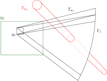
?figurename? 9: The geometry in Lemma 2.14

Proof:.

We only show (i), the proof of (ii) being analogous. Set

$$\Gamma_{1}=\bigcup\Big{\{}T_{w_{1}}:w_{1}\in\left[W_{1}^{\lambda_{1},\mu,\not\sim b}(q_{0})\right]^{\Pi_{v_{1},v_{2}}}\Big{\}}\setminus 5b,\quad Q^{\mu}_{\Gamma_{1}}=\{q\in Q^{\mu}|R^{\delta}q\cap\Gamma_{1}\neq\emptyset\}.$$

Since we have seen in Lemma 2.8 (iv) that $T_{w_{2}}$ is transversal to $\Gamma_{1},$ we have

$$|Q^{\mu}_{\Gamma_{1}}\cap Q^{\mu}(w_{2})|\lesssim R^{c\delta}.$$ (2.40)

Due to the separation of the tube directions, the sets $T_{w_{1}}\setminus 5b$ do not overlap too much. To be more precise, we claim that for all cubes $q\in Q^{\mu}_{\Gamma_{1}}$

$$\Big{|}\Big{\{}w_{1}\in\left[W_{1}^{\lambda_{1},\mu,\not\sim b}(q_{0})\right]^{\Pi_{v_{1},v_{2}}}:R^{\delta}q\cap T_{w_{1}}\setminus 5b\neq\emptyset\big{\}}\Big{|}\lesssim R^{c\delta}.$$ (2.41)

Indeed, let $w_{1},w^{\prime}_{1}\in\left[W_{1}^{\lambda_{1},\mu,\not\sim b}(q_{0})\right]^{\Pi_{v_{1},v_{2}}}$ and $x\in R^{\delta}q\cap T_{w_{1}}\setminus 5b$, $x^{\prime}\in R^{\delta}q\cap T_{w^{\prime}_{1}}\setminus 5b$. The definition of $W_{1}(q_{0})$ means that we find $x_{0}\in R^{\delta}q_{0}\cap T_{w_{1}}$ and $x^{\prime}_{0}\in R^{\delta}q_{0}\cap T_{w^{\prime}_{1}}$; then we may write

$$x=x_{0}+|x-x_{0}|N(v_{1})+\mathcal{O}(R^{\prime})\text{ and }x^{\prime}=x^{\prime}_{0}+|x^{\prime}-x^{\prime}_{0}|N_{0}(v^{\prime}_{1})+\mathcal{O}(R^{\prime}).$$ (2.42)

Furthermore we have

$$\big{|}|x-x_{0}|-|x^{\prime}-x^{\prime}_{0}|\big{|}\leq|x-x^{\prime}|+|x_{0}-x^{\prime}_{0}|=\mathcal{O}(R^{c\delta}R^{\prime}).$$ (2.43)

Since $T_{w_{1}}$ has length ${R^{\prime 2}}/{\kappa^{(1)}}$, so that the length of $b$ in the direction of $T_{w_{1}}$ is at least $R^{-2\delta}{R^{\prime 2}}/{\kappa^{(1)}}$, and since $x_{0}\in R^{\delta}q_{0}\subset 4b$ but $x\notin 5b$, we conclude that

$$R^{-2\delta}\frac{R^{\prime 2}}{\kappa^{(1)}}\leq|x-x_{0}|.$$ (2.44)

Applying Lemma 2.5, and making consecutively use of the estimates (2.44), (2.43), (2.42) and again (2.43), we obtain

$$R^{\prime}|v_{1}-v^{\prime}_{1}| \lesssim \frac{R^{\prime}}{\kappa^{(1)}}|N(v_{1})-N(v^{\prime}_{1})|$$

$$\lesssim R^{2\delta}R^{\prime-1}|x-x_{0}|\,|N_{0}(v_{1})-N_{0}(v^{\prime}_{1})|$$

$$\lesssim R^{2\delta}R^{\prime-1}\big{|}|x-x_{0}|N_{0}(v_{1})-|x^{\prime}-x^{\prime}_{0}|N_{0}(v^{\prime}_{1})\big{|}+\mathcal{O}(R^{c\delta})$$

$$\lesssim R^{2\delta}R^{\prime-1}\big{(}|x-x^{\prime}|+|x^{\prime}_{0}-x_{0}|\big{)}+\mathcal{O}(R^{c\delta})$$

$$= \mathcal{O}(R^{c\delta}).$$

Recall also that the direction of a tube $T_{w_{1}}$ with $w_{1}=(y_{1},v_{1})$ depends only on $v_{1},$ and thus the set of all these directions corresponding to the set

$$\Big{\{}w_{1}\in\left[W_{1}^{\lambda_{1},\mu,\not\sim b}(q_{0})\right]^{\Pi_{v_{1},v_{2}}}:R^{\delta}q\cap T_{w_{1}}\setminus 5b\Big{\}}$$

has cardinality $\mathcal{O}(R^{c\delta})$. But, for a fixed direction $v_{1}$, the number of parameters $y_{1}$ such that the tube $T_{(y_{1},v_{1})}$ passes through $R^{c\delta}q_{0}$ is bounded by $\mathcal{O}(R^{c\delta})$ anyway, and thus (2.41) holds true.

Recall next from (2.38) that for $w_{1}\not\sim b$ we have $R^{-c\delta}|Q^{\mu}(w_{1})|\lesssim|\{q\in Q^{\mu}(w_{1}):q\cap 5b=\emptyset\}|.$ Since for $w_{1}\in W_{1}^{\lambda_{1},\mu}$ we have $|Q^{\mu}(w_{1})|\sim\lambda_{1},$ we may thus estimate

$$R^{-c\delta}\lambda_{1}\left|\left[W_{1}^{\lambda_{1},\mu,\not\sim b}(q_{0})\right]^{\Pi_{v_{1},v_{2}}}\right|$$

$$\lesssim R^{-c\delta}\sum_{w_{1}\in\left[W_{1}^{\lambda_{1},\mu,\not\sim b}(q_{0})\right]^{\Pi_{v_{1},v_{2}}}}|Q^{\mu}(w_{1})|$$

$$\lesssim \sum_{w_{1}\in\left[W_{1}^{\lambda_{1},\mu,\not\sim b}(q_{0})\right]^{\Pi_{v_{1},v_{2}}}}|\{q\in Q^{\mu}(w_{1}):q\cap 5b=\emptyset\}|$$

$$\leq \sum_{w_{1}\in\left[W_{1}^{\lambda_{1},\mu,\not\sim b}(q_{0})\right]^{\Pi_{v_{1},v_{2}}}}|\{q\in Q^{\mu}:R^{\delta}q\cap T_{w_{1}}\neq\emptyset,\ R^{\delta}q\cap 5b=\emptyset\}|$$

$$\leq \sum_{w_{1}\in\left[W_{1}^{\lambda_{1},\mu,\not\sim b}(q_{0})\right]^{\Pi_{v_{1},v_{2}}}}|\{q\in Q^{\mu}:R^{\delta}q\cap(T_{w_{1}}\setminus 5b)\neq\emptyset\}|$$

$$= \sum_{q\in Q^{\mu}}\Big{|}\Big{\{}w_{1}\in\left[W_{1}^{\lambda_{1},\mu,\not\sim b}(q_{0})\right]^{\Pi_{v_{1},v_{2}}}:R^{\delta}q\cap(T_{w_{1}}\setminus 5b)\neq\emptyset\Big{\}}\Big{|}$$

$$= R^{c\delta}|Q^{\mu}_{\Gamma_{1}}|,$$

where we have used (2.41) in the last estimate. But, by (2.40), we also have

$$\mu_{2}|Q^{\mu}_{\Gamma_{1}}|=\sum_{q\in Q^{\mu}_{\Gamma_{1}}}|W_{2}(q)|\leq\sum_{w_{2}\in W_{2}}|Q^{\mu}_{\Gamma_{1}}\cap Q^{\mu}(w_{2})|\lesssim R^{c\delta}|W_{2}|,$$

and combining this with the previous estimate we arrive at the desired estimate in (i). $\Box$

Lemma 2.15.

Let $0<\delta<\frac{1}{4}$. Then

$$II =\sum_{b}\|\sum_{w_{1}\in W_{1}^{\lambda_{1},\mu,\not\sim b}}p_{w_{1}}\sum_{w_{2}\in W_{2}^{\lambda_{2},\mu}}p_{w_{2}}\sum_{q\in Q^{\mu}}\chi_{q}\|_{L^{p}(b)}$$

$$\leq C_{\alpha}R^{c\delta}(\kappa^{1}\kappa^{2})^{\frac{1}{2}-\frac{1}{p}}D^{3-\frac{5}{p}}|W_{1}|^{\frac{1}{2}}|W_{2}|^{\frac{1}{2}}$$ (2.45)

and

$$III =\sum_{b}\|\sum_{w_{1}\in W_{1}^{\lambda_{1},\mu,\sim b}}p_{w_{1}}\sum_{w_{2}\in W_{2}^{\lambda_{2},\mu,\not\sim b}}p_{w_{2}}\sum_{q\in Q^{\mu}}\chi_{q}\|_{L^{p}(b)}$$

$$\leq C_{\alpha}R^{c\delta}(\kappa^{1}\kappa^{2})^{\frac{1}{2}-\frac{1}{p}}D^{3-\frac{5}{p}}|W_{1}|^{\frac{1}{2}}|W_{2}|^{\frac{1}{2}}.$$ (2.46)

Proof:.

We will only prove the first inequality; the proof of second one works in a similar way. Since the number of $b$’s over which we sum in (2.45) is of the order $R^{c\delta}$, it is enough to show that for every fixed $b$

$$\|\sum_{w_{1}\in W_{1}^{\lambda_{1},\mu,\not\sim b}}p_{w_{1}}\sum_{w_{2}\in W_{2}^{\lambda_{2},\mu}}p_{w_{2}}\sum_{q\in Q^{\mu}}\chi_{q}\|_{L^{p}(b)}\leq C_{\alpha}R^{c\delta}(\kappa^{1}\kappa^{2})^{\frac{1}{2}-\frac{1}{p}}D^{3-\frac{5}{p}}|W_{1}|^{\frac{1}{2}}|W_{2}|^{\frac{1}{2}}.$$ (2.47)

For $p=1$, we apply (2.35) from Lemma 2.10:

$$\|\sum_{w_{1}\in W_{1}^{\lambda_{1},\mu,\not\sim b}}p_{w_{1}}\sum_{w_{2}\in W_{2}^{\lambda_{2},\mu}}p_{w_{2}}\sum_{q\in Q^{\mu}}\chi_{q}\|_{L^{1}(b)}$$

$$\lesssim \|\sum_{w_{1}\in W_{1}^{\lambda_{1},\mu,\not\sim b}}p_{w_{1}}\sum_{w_{2}\in W_{2}^{\lambda_{2},\mu}}p_{w_{2}}\|_{L^{1}(Q_{S_{1},S_{2}}(R))}$$

$$\leq \frac{R^{\prime 2}}{\sqrt{\kappa^{(1)}\kappa^{(2)}}}|W_{1}|^{\frac{1}{2}}|W_{1}|^{\frac{1}{2}}.$$

For $p=2$, we claim that

$$\|\sum_{w_{1}\in W_{1}^{\lambda_{1},\mu,\not\sim b}}p_{w_{1}}\sum_{w_{2}\in W_{2}^{\lambda_{2},\mu}}p_{w_{2}}\sum_{q\in Q^{\mu}}\chi_{q}\|_{L^{2}(b)}^{2}\lesssim C_{\alpha}R^{c\delta}R^{\prime-1}|W_{1}||W_{2}|.$$ (2.48)

The desired inequality (2.45) will then follow by means of interpolation with the previous $L^{1}$-estimate - notice here that $R^{\frac{5}{p}-3}\leq 1$ since $\frac{5}{3}\leq p$.

To prove (2.48), recall that the side lengths of $b$ are of the form $(R^{\prime 2}/\kappa^{(j)})R^{-2\delta}=R^{\prime}/(D\kappa^{(j)})R^{1-2\delta}\geq R^{\prime}R^{1-2\delta}$, $j\in\{1,2\}$. If $q\cap 2b=\emptyset$, then for $x\in b$ we have $|x-c_{q}|\geq\inf\limits_{y\notin 2b}|x-y|=\mathop{d}(x,(2b)^{c})\geq R^{\prime}R^{1-2\delta}$. Therefore for every $x\in b$

$$\big{|}\sum_{q\in Q^{\mu},q\cap 2b=\emptyset}\chi_{q}(x)\big{|}\leq C_{N}\underset{2^{l}\geq R^{1-2\delta}}{\sum_{l\in\mathbbm{N}}}\ \underset{|x-c_{q}|\sim R^{\prime}2^{l}}{\sum_{q\in Q^{\mu}}}\left(1+\frac{|x-c_{q}|}{R^{\prime}}\right)^{-N-2}$$

$$\lesssim C_{N}\underset{2^{l}\geq R^{1-2\delta}}{\sum_{l\in\mathbbm{N}}}|\{q:|x-c_{q}|\sim R^{\prime}2^{l}\}|\,2^{-(N+2)l}$$

$$\sim C_{N}\underset{2^{l}\geq R^{1-2\delta}}{\sum_{l\in\mathbbm{N}}}2^{-Nl}\sim C_{N}R^{-(1-2\delta)N}=C_{\delta,N^{\prime}}R^{-N^{\prime}}.$$ (2.49)

The last step requires that $\delta<1/2.$ Choosing $N$ sufficiently large, we see that by Lemma 2.10 and Lemma 2.11

$$\Big{\|}\sum_{w_{1}\in W_{1}^{\lambda_{1},\mu,\not\sim b}}p_{w_{1}}\sum_{w_{2}\in W_{2}^{\lambda_{2},\mu}}p_{w_{2}}\sum_{q\in Q^{\mu},q\cap 2b=\emptyset}\chi_{q}\Big{\|}_{L^{2}(b)}^{2}$$

$$\lesssim \Big{\|}\sum_{w_{1}\in W_{1}^{\lambda_{1},\mu,\not\sim b}}p_{w_{1}}\sum_{w_{2}\in W_{2}^{\lambda_{2},\mu}}p_{w_{2}}\Big{\|}_{L^{2}}^{2}\,\cdot\,\Big{\|}\sum_{q\in Q^{\mu},q\cap 2b=\emptyset}\chi_{q}\Big{\|}_{L^{\infty}(b)}^{2}$$

$$\lesssim C_{\delta,N^{\prime}}R^{\prime-1}|W_{1}|\,|W_{2}|\min\limits_{j}\sup\limits_{v_{1},v_{2}}|V_{j}^{\Pi_{v_{1},v_{2}}}|R^{-2N^{\prime}}$$

$$\lesssim C_{\delta,N^{\prime}}R^{\prime-1}|W_{1}|\,|W_{2}|R^{1-2N^{\prime}}$$

$$\lesssim C^{\prime}_{\delta,N^{\prime\prime}}R^{\prime-1}|W_{1}|\,|W_{2}|R^{-N^{\prime\prime}}.$$

Thus it is enough to consider the sum over the set $Q^{\mu}_{b}=\{q\in Q^{\mu}:q\cap 2b\neq\emptyset\}$. For fixed $w_{1},w_{2},$ we split this set into the subsets $Q^{\mu}_{b}(w_{1},w_{2})=Q^{\mu}_{b}\cap Q^{\mu}(w_{1})\cap Q^{\mu}(w_{2}),$ $Q^{\mu}_{b}\cap Q^{\mu}(w_{1})\setminus Q^{\mu}(w_{2})$ and

$$Q^{\mu}_{b}\setminus Q^{\mu}(w_{1})=\big{(}Q^{\mu}_{b}\cap Q^{\mu}(w_{2})\setminus Q^{\mu}(w_{1})\big{)}\cup\big{(}Q^{\mu}_{b}\setminus(Q^{\mu}(w_{2})\cap Q^{\mu}(w_{1}))\big{)}.$$

Except for the first set, the contributions by the other subsets can be treated in the same way, since they are all special cases of the following situation:

Let $Q_{0}=Q_{0}(w_{1},w_{2})\subset Q^{\mu}_{b}$ such that there exists an $j\in\{1,2\}$ with $R^{\delta}q\cap T_{w_{j}}=\emptyset$ for all $q\in Q_{0}$. Then

$$\|\sum_{w_{1}\in W_{1}^{\lambda_{1},\mu,\not\sim b}}p_{w_{1}}\sum_{w_{2}\in W_{2}^{\lambda_{2},\mu}}p_{w_{2}}\sum_{q\in Q_{0}}\chi_{q}\|_{L^{2}(b)}^{2}\lesssim C_{\alpha}R^{c\delta}R^{\prime-1}|W_{1}||W_{2}|.$$ (2.50)

Notice that the right-hand side is just what we need for (2.48).

For the proof of (2.50), assume without loss of generality that $j=1$. Let $q\in Q_{0}.$ Then $T_{w_{1}}\cap R^{\delta}q=\emptyset,$ and for all $x\in(R^{\delta}/2)q$ we have $(R^{\delta}/2)R^{\prime}\leq\text{\rm dist\,}(x,(R^{\delta}q)^{c})\leq\text{\rm dist\,}(x,T_{w_{1}})$. Thus for every $x\in Q_{S_{1},S_{2}}(R)$, we have $\text{\rm dist\,}(x,T_{w_{1}})\geq(R^{\delta}/2)R^{\prime}$ or $x\notin(R^{\delta}/2)q$. In the first case, we have

$$|p_{w_{1}}(x)|\leq C_{N}R^{\prime-1}\left(1+\frac{\text{\rm dist\,}(x,T_{w_{1}})}{R^{\prime}}\right)^{-2N}$$ (2.51)

$$\leq C^{\prime}_{N}R^{\prime-1}R^{-\delta N}\left(1+\frac{\text{\rm dist\,}(x,T_{w_{1}})}{R^{\prime}}\right)^{-N}.$$

One the other hand, in the second case, where $x\notin(R^{\delta}/2)q,$ we have $(R^{\delta}/2)R^{\prime}\leq|x-c_{q}|$. Using the rapid decay of the Schwartz function $\phi$ we then see that

$$|\chi_{q}(x)|=|\chi\left(\frac{x-c_{q}}{R^{\prime}}\right)|\leq C_{N}\left(\frac{|x-c_{q}|}{R^{\prime}}\right)^{-N}\leq C^{\prime}_{N}R^{-\delta N}.$$ (2.52)

Applying an argument similar to the one used in (2.49), we even obtain

$$|\sum_{q\in Q_{0}}\chi_{q}(x)|\leq C^{\prime\prime}_{N}R^{-\delta N}$$

for all $x\notin(R^{\delta}/2)q$. To summarize, we obtain for that for every $x\in Q_{S_{1},S_{2}}(R)$

$$\big{|}p_{w_{1}}\sum_{q\in Q_{0}(w_{1},w_{2})}\chi_{q}\big{|}(x)\leq C(N,\delta)R^{\prime-1}R^{-\delta N}\left(1+\frac{\text{\rm dist\,}(x,T_{w_{1}})}{R^{\prime}}\right)^{-N}.$$ (2.53)

This means that the expression $p_{w_{1}}\sum_{q\in Q_{0}(w_{1},w_{2})}\chi_{q}$ can not only be estimated in the same way as the original wave packet $p_{w_{1}},$ but we even obtain an improved estimate because of an additional factor $R^{-\delta N}$. If we replace $p_{w_{1}}$ by $p_{w_{2}}$ on the left-hand side, we obtain in a similar way just the standard wave packet estimate

$$\big{|}p_{w_{2}}\sum_{q\in Q_{0}(w_{1},w_{2})}\chi_{q}\big{|}(x)\lesssim\|p_{w_{2}}\|_{\infty}\lesssim R^{\prime-1}\left(1+\frac{\text{\rm dist\,}(x,T_{w_{2}})}{R^{\prime}}\right)^{-N},$$ (2.54)

without an additional factor.

We can now finish the proof of (2.50), basically by following the ideas of the proof of the estimate (2.36) in Lemma 2.10. The crucial argument was the fact that the Fourier transform of $p_{w^{\prime}_{j+1}}p_{w_{j}}$ is supported in $v^{\prime}_{j+1}+v_{j}+\mathcal{O}(R^{\prime-1})$. Since $\text{\rm supp\,}\widehat{\chi_{q}}=\text{\rm supp\,}\hat{\chi}(R^{\prime}\cdot)\subset B(0,R^{\prime-1})$, the Fourier support of $p_{w_{1}}p_{w_{2}}\sum\limits_{q\in Q_{0}(w_{1},w_{2})}\chi_{q}$ remains essentially the same. It is at this point that we need that the functions $\chi_{q}$ have compact Fourier support. The modified wave packets $p_{w_{i}}\sum\limits_{q\in Q_{0}(w_{1},w_{2})}\chi_{q}$ are still well separated with respect to the parameter $y_{i},$ for fixed direction $v_{i},$ thanks to (2.53) and (2.54). Thus the argument from Lemma 2.10 applies, and by the analogue of (2.37) we obtain

$$\big{\|}\underset{w_{2}\in W_{2}^{\lambda_{2},\mu}}{\underset{w_{1}\in W_{1}^{\lambda_{1},\mu,\not\sim b}}{\sum}}p_{w_{1}}p_{w_{2}}\sum_{q\in Q_{0}(w_{1},w_{2})}\chi_{q}\big{\|}_{L^{2}(b)}^{2}\lesssim R^{\prime}|W_{1}|\ |W_{2}|\ \min_{j}\sup_{v_{1},v_{2}}|V_{j}^{\Pi_{v_{1},v_{2}}}|$$

$$\times\sup\limits_{w_{1}\in W_{1},w^{\prime}_{2}\in W_{2}}\|p_{w^{\prime}_{2}}\sum_{q\in Q_{0}(w_{1},w^{\prime}_{2})}\chi_{q}\|_{\infty}\sup\limits_{w^{\prime}_{1}\in W_{1},w_{2}\in W_{2}}\|p_{w^{\prime}_{1}}\sum_{q\in Q_{0}(w^{\prime}_{1},w_{2})}\chi_{q}\|_{\infty}$$

$$\lesssim C_{\delta,N^{\prime}}R^{\prime-1}|W_{1}|\ |W_{2}|\ \min_{j}\sup_{v_{1},v_{2}}|V_{j}^{\Pi_{v_{1},v_{2}}}|R^{-N^{\prime}}$$

$$\lesssim C_{\delta,N^{\prime}}R^{\prime-1}R^{1-N^{\prime}}|W_{1}|\ |W_{2}|.$$

In the second inequality, we have made use of (2.53) and (2.54), and the last one is based on Lemma 2.11. This concludes the proof of (2.50).

What remains to be controlled are the contributions by the cubes $q$ from $Q^{\mu}_{b}(w_{1},w_{2})$. Notice that the kernel $K(q,q^{\prime})=\chi_{q}(x)\chi_{q^{\prime}}(x)$ satisfies Schur’s test condition

$$\sup_{q}\sum_{q^{\prime}}\chi_{q}(x)\chi_{q^{\prime}}(x)\lesssim\sum_{q^{\prime}}\chi_{q^{\prime}}(x)\lesssim 1,$$

with a constant not depending in $x.$ Let us put $f_{q}=\underset{w_{2}\in W_{2}^{\lambda_{2},\mu}(q)}{\underset{w_{1}\in W_{1}^{\lambda_{1},\mu,\not\sim b}(q)}{\sum}}p_{w_{1}}p_{w_{2}},$ and observe that for $w_{1}\in W_{1}^{\lambda_{1},\mu,\not\sim b}$ and $w_{2}\in W_{2}^{\lambda_{2},\mu},$ we have $q\in Q^{\mu}_{b}(w_{1},w_{2})$ if and only if $q\in Q^{\mu}_{b}$ and $w_{1}\in W_{1}^{\lambda_{1},\mu,\not\sim b}(q)$ and $w_{2}\in W_{2}^{\lambda_{2},\mu}(q).$ Then we see that we may estimate

$$\|\underset{w_{2}\in W_{2}^{\lambda_{2},\mu}}{\underset{w_{1}\in W_{1}^{\lambda_{1},\mu,\not\sim b}}{\sum}}p_{w_{1}}p_{w_{2}}\sum_{q\in Q^{\mu}_{b}(w_{1},w_{2})}\chi_{q}\|_{L^{2}(b)}^{2}=\|\sum_{q\in Q^{\mu}_{b}}\chi_{q}f_{q}\|_{L^{2}(b)}^{2}$$

$$= \int_{b}\big{|}\sum_{q,q^{\prime}\in Q^{\mu}_{b}}\chi_{q}\chi_{q^{\prime}}f_{q}f_{q^{\prime}}\big{|}dx=\int_{b}\big{|}\sum_{q,q^{\prime}\in Q^{\mu}_{b}}K(q,q^{\prime})f_{q}f_{q^{\prime}}\big{|}dx$$

$$\lesssim \int_{b}\sum_{q\in Q^{\mu}_{b}}|f_{q}|^{2}\,dx=\sum_{q\in Q^{\mu},q\cap 2b\neq\emptyset}\|\underset{w_{2}\in W_{2}^{\lambda_{2},\mu}(q)}{\underset{w_{1}\in W_{1}^{\lambda_{1},\mu,\not\sim b}(q)}{\sum}}p_{w_{1}}p_{w_{2}}\|_{L^{2}(b)}^{2}.$$

Invoking also Lemma 2.10 and Lemma 2.14 (i), we thus obtain

$$\|\underset{w_{2}\in W_{2}^{\lambda_{2},\mu}}{\underset{w_{1}\in W_{1}^{\lambda_{1},\mu,\not\sim b}}{\sum}}p_{w_{1}}p_{w_{2}}\sum_{q\in Q^{\mu}_{b}(w_{1},w_{2})}\chi_{q}\|_{L^{2}(b)}^{2}$$

$$\lesssim \sum_{q\in Q^{\mu},q\cap 2b\neq\emptyset}R^{\prime-1}|W_{1}^{\lambda_{1},\mu,\not\sim b}(q)|\ |W_{2}^{\lambda_{2},\mu}(q)|\sup_{v_{1},v_{2}}\big{|}[W_{1}^{\lambda_{1},\mu,\not\sim b}(q)]^{\Pi_{v_{1},v_{2}}}\big{|}$$

$$\lesssim R^{c\delta}R^{\prime-1}\sum_{q\in Q^{\mu},q\cap 2b\neq\emptyset}|W_{1}^{\lambda_{1},\mu}(q)|\ |W_{2}(q)|\frac{|W_{2}|}{\lambda_{1}\mu_{2}}$$

$$\lesssim R^{c\delta}R^{\prime-1}\sum_{w_{1}\in W_{1}^{\lambda_{1},\mu}}|Q^{\mu}(w_{1})|\frac{|W_{2}|}{\lambda_{1}}$$

$$\lesssim R^{c\delta}R^{\prime-1}|W_{1}|\ |W_{2}|.$$

This completes the proof of estimate (2.45), hence of Lemma 2.15. $\Box$

2.8 Induction on scales

We can now easily complete the proof of Theorem 2.6 by following standard arguments.

Corollary 2.16.

There exist constants $c,\delta_{0}>0$ such that $c\delta_{0}>1$ and such that the following holds true:

Whenever $\alpha>0$ is such that $E(\alpha)$ holds true, then $E(\max\{\alpha(1-\delta),c\delta\})$ holds true for every $\delta$ such that $0<\delta<\delta_{0}.$

Proof:.

Let us put $\delta_{0}=1/4.$ Then the previous Lemmas 2.13 and 2.15 imply that

$$\big{\|}\prod_{j=1,2}\sum_{w_{j}\in W_{j}^{\lambda_{j},\mu}}p_{w_{j}}\sum_{q\in Q^{\mu}}\chi_{q}\big{\|}_{L^{p}(Q_{S_{1},S_{2}}(R))}\leq I+II+III$$

$$\lesssim \big{(}C_{\alpha}R^{\alpha(1-\delta)}\log^{\gamma_{\alpha}}(1+R)+C_{\delta}R^{c\delta}\big{)}(\kappa^{1}\kappa^{2})^{\frac{1}{2}-\frac{1}{p}}D^{3-\frac{5}{p}}\log^{\gamma_{\alpha}}(C_{0})|W_{1}|^{\frac{1}{2}}|W_{2}|^{\frac{1}{2}}$$

$$\lesssim C_{\alpha,\delta}R^{\alpha(1-\delta)\vee c\delta}\log^{\gamma_{\alpha}}(1+R)(\kappa^{1}\kappa^{2})^{\frac{1}{2}-\frac{1}{p}}D^{3-\frac{5}{p}}\log^{\gamma_{\alpha}}(C_{0})|W_{1}|^{\frac{1}{2}}|W_{2}|^{\frac{1}{2}}$$

whenever $\delta<\delta_{0},$ where $C_{0}=C_{0}(S)\gtrsim 1$ is defined in (2.20). By Lemma 2.9, this estimate implies $E(\alpha(1-\delta)\vee c\delta).$ Finally, by simply increasing the constant $c,$ if necessary, we may also ensure that $c\delta_{0}>1.$ $\Box$

Corollary 2.17.

$E(\alpha)$ holds true for every $\alpha>0.$

This completes also the proof of Theorem 2.6.

Proof:.

Define inductively the sequence $\alpha_{0}=1$, $\alpha_{j+1}=c\alpha_{j}/(c+\alpha_{j}),$ which is decreasing and converges to $0.$ It therefore suffices to prove that $E(\alpha_{j})$ is valid for every $j\in\mathbbm{N}$. But, by Corollary 2.12, $E(\alpha_{0})=E(1)$ does hold true. Moreover, Corollary 2.16 shows that $E(\alpha_{j})$ implies $E(\alpha_{j+1}),$ for if we choose $\delta=\alpha_{j}/(c+\alpha_{j}),$ then $\delta<1/c<\delta_{0}$ and $\alpha_{j}(1-\delta)=c\delta=\alpha_{j}c/(c+\alpha_{j})=\alpha_{j+1},$ and thus we may conclude by induction. $\Box$

3 Scaling

For the proof of our main theorem, we shall have to perform a kind of Whitney type decomposition of $S\times S$ into pairs of patches of hypersurfacec $(S_{1},S_{2})$ and prove very precise bilinear restriction estimates for those. In order to reduce these estimates to Theorem 2.2, we shall need to rescale simultanously the hypersurfaces $S_{1},S_{2}$ for each such pair $(S_{1},S_{2})$ in a suitable way. To this end, we shall denote here and in the sequel by $R^{*}_{S_{1},S_{2}}$ the bilinear Fourier extension operator

$$R^{*}_{S_{1},S_{2}}(f_{1},f_{2})=R^{*}_{\mathbbm{R}^{2}}f_{1}\cdot R^{*}_{\mathbbm{R}^{2}}f_{2},\qquad f_{1}\in L^{2}(U_{1}),f_{2}\in L^{2}(U_{2})$$

associated to any pair of hypersurfaces $(S_{1},S_{2})$ given as the graphs $S_{j}=\{(\xi,\phi_{j}(\xi)):\xi\in U_{j}\},j=1,2.$

The following trivial lemma comprises the effect of the type of rescaling that we shall need.

Lemma 3.1.

Let $S_{j}=\{(\xi,\phi(\xi):\xi\in U_{j}\}$, where again $U_{j}\subset\mathbbm{R}^{d}$ is open and bounded for $j=1,2$. Let $A\in GL(d,\mathbbm{R})$, $a>0$, put $\phi^{s}(\eta)=\frac{1}{a}\phi(A\eta),$ and let

$$S_{j}^{s}=\{(\eta,\phi^{s}(\eta))|\eta\in U_{j}^{s}\},\quad U_{j}^{s}=A^{-1}(U_{j}),\quad j=1,2.$$

For any measurable subset $Q^{s}\subset\mathbbm{R}^{d+1}$, we set $Q=\{x:({\,}^{t}Ax^{\prime},ax_{d+1})\in Q^{s}\}$. Assume that the following estimate holds true:

$$\|R^{*}_{S^{s}_{1},S^{s}_{2}}(g_{1},g_{2})\|_{L^{p}(Q^{s})}\leq C_{s}\|g_{1}\|_{2}\|g_{2}\|_{2}\quad\text{ for all }g_{j}\in L^{2}(U^{s}_{j}).$$

Then

$$\|R^{*}_{S_{1},S_{2}}(f_{1},f_{2})\|_{L^{p}(Q)}\leq C_{s}|\det A|^{\frac{1}{p^{\prime}}}a^{-\frac{1}{p}}\|f_{1}\|_{2}\|f_{2}\|_{2}\quad\text{ for all }f_{j}\in L^{2}(U_{j}).$$

We now return to our model hypersurface (compare (1.3), (1.4) and (1.4)), which is the graph of

$$\phi(\xi_{1},\xi_{2})=\psi_{1}(\xi_{1})+\psi_{2}(\xi_{2})$$

on $]0,1[\times]0,1[,$ where the derivatives of the $\psi_{i}$ satisfy

$$\psi_{i}^{\prime\prime}(\xi_{i}) \sim\xi_{i}^{m_{i}-2},$$

$$|\psi_{i}^{(k)}(\xi_{i})| \lesssim\xi_{i}^{m_{i}-k}\quad\mbox{for }\ k\geq 3,$$

and where $m_{1},m_{2}\in\mathbbm{R}$ are such that $m_{i}\geq 2.$

We shall apply the preceding lemma to pairs $S_{1}=S$ and $S_{2}=\tilde{S}$ of patches of this hypersurface on which the following assumptions are met:

GENERAL ASSUMPTIONS: Let $S=\{(\xi,\phi(\xi)):\xi\in U\}$ and $\tilde{S}=\{(\xi,\phi(\xi)):\xi\in\tilde{U}\},$ where $U=r+[0,d_{1}]\times[0,d_{2}]$ and $\tilde{U}=\tilde{r}+[0,\tilde{d}_{1}]\times[0,\tilde{d}_{2}],$ with $r=(r_{1},r_{2})$ and $\tilde{r}=(\tilde{r}_{1},\tilde{r}_{2}).$

We assume that for $i=1,2$ we have $r_{i}\geq d_{i}$ and $\tilde{r}_{i}\geq\tilde{d}_{i},$ so that the principal curvature $\psi_{i}^{\prime\prime}$ of $S$ with respect to $\xi_{i}$ is comparable to $\kappa_{i}=r_{i}^{m_{i}-2}$, and that of $\tilde{S}$ is comparable to $\tilde{\kappa}_{i}=\tilde{r}_{i}^{m_{i}-2}.$ We put

$$\bar{d}_{i}=d_{i}\vee\tilde{d}_{i},$$

$$\kappa=\kappa_{1}\vee\kappa_{2},\quad\tilde{\kappa}=\tilde{\kappa}_{1}\vee\tilde{\kappa}_{2},$$

$$\bar{\kappa}_{i}=\kappa_{i}\vee\tilde{\kappa}_{i},\quad\bar{r}_{i}=r_{i}\vee\tilde{r}_{i}$$ (3.1)

$$\bar{\kappa}=\kappa\vee\tilde{\kappa}=\bar{\kappa}_{1}\vee\bar{\kappa}_{2},$$

$$\Delta r_{i}=r_{i}-\tilde{r}_{i}.$$

In addition, we assume that for every direction $\xi_{i},i=1,2,$ the rectangle $U$ respectively $\tilde{U}$ on which the corresponding principal curvature is bigger (which means that its projection to the $\xi_{i}$-axis is the one further to the right), has also bigger length in this direction. This is easily seen to be equivalent to

$$(\kappa_{i}d_{i})\vee(\tilde{\kappa}_{i}\tilde{d}_{i})=\bar{\kappa}_{i}\bar{d}_{i}.$$ (3.2)

Last, but not least, we assume the rectangles $U$ and $\tilde{U}$ are separated with respect to both variables $\xi_{i},i=1,2,$ in the following sense:

$${\rm dist}_{\xi_{i}}(U,\tilde{U})=\inf\{|\xi_{i}-\tilde{\xi}_{i}|:\xi\in U,\tilde{\xi}\in\tilde{U}\}\sim|\Delta r_{i}|\sim\bar{d}_{i}.$$ (3.3)

Given these assumptions, we shall introduce a rescaling as follows: we put

$$a_{1}=\bar{\kappa}_{2}\bar{d}_{2},\qquad a_{2}=\bar{\kappa}_{1}\bar{d}_{1},$$ (3.4)

and

$$\phi^{s}(\eta)=\frac{1}{a}\phi(A\eta)=\frac{1}{a_{1}a_{2}}\phi(a_{1}\eta_{1},a_{2}\eta_{2}).$$ (3.5)

The quantities that arise after this scaling will be denoted by a superscript $s,$ i.e.,

$$r_{i}^{s}=\frac{r_{i}}{a_{i}},\quad d_{i}^{s}=\frac{d_{i}}{a_{i}},\quad D^{s}=\min\{d_{1}^{s},d_{2}^{s},\tilde{d}_{1}^{s},\tilde{d}_{2}^{s}\},$$

$$\kappa_{i}^{s}=\frac{1}{a_{1}a_{2}}a_{i}^{2}\kappa_{i}=\frac{a_{i}}{a_{i+1\,{\rm mod}2}}\kappa_{i},$$

$$U^{s}=r^{s}+[0,d^{s}_{1}]\times[0,d^{s}_{2}],$$

with corresponding expressions for $\tilde{r}^{s},\tilde{d}_{i}^{s},\tilde{\kappa}^{s}_{i}$ and $\tilde{U}^{s}.$ For later use, recall also the normal field $N$ on $S\cup\tilde{S}$ defined by $N(\xi,\phi(\xi))=(-\nabla\phi(\xi),1)$ and the coresponding unit normal field $N_{0}={N}/{|N|}.$ After scaling, the corresponing normal fields on $S^{s}\cup\tilde{S}^{s}$ will be denoted by $N^{s}$ and $N_{0}^{s}.$ With our choice of scaling, the following lemma holds true:

Lemma 3.2 (Scaling).

1. For $i=1,2$ and all $\eta\in U^{s}$ and $\tilde{\eta}\in\tilde{U}^{s}$ we have $|\partial_{i}\phi^{s}(\eta)-\partial_{i}\phi^{s}(r^{s})|\lesssim\kappa_{i}^{s}d_{i}^{s}\lesssim 1$ and $|\partial_{i}\phi^{s}(\tilde{\eta})-\partial_{i}\phi^{s}(\tilde{r}^{s})|\lesssim\tilde{\kappa}_{i}^{s}\tilde{d}_{i}^{s}\lesssim 1$. Moreover, $\bar{\kappa}_{i}^{s}\bar{d}_{i}^{s}=1.$

2. $|\partial^{\alpha}\phi^{s}(\eta)|\lesssim\kappa^{s}|d_{1}^{s}\wedge d_{2}^{s}|^{2-|\alpha|}$  for every $|\alpha|\geq 2$, $\eta\in U^{s}$;
   $|\partial^{\alpha}\phi^{s}(\tilde{\eta})|\lesssim\tilde{\kappa}^{s}|\tilde{d}_{1}^{s}\wedge\tilde{d}_{2}^{s}|^{2-|\alpha|}$ for every $|\alpha|\geq 2$, $\tilde{\eta}\in\tilde{U}^{s}$.

3. For $i=1,2,$ i.e., with respect to both variables, the separation condition

   $$|\partial_{i}\phi^{s}(\eta)-\partial_{i}\phi^{s}(\tilde{\eta})|\sim 1\quad\mbox{ for all }\eta\in S,\tilde{\eta}\in\tilde{S}.$$

   holds true.

In particular, the rescaled pair of hypersurfaces $(S^{s},\tilde{S}^{s})$ satisfies the general assumptions (i) –(iii) made in Theorem 2.6.

Proof:.

Observe first that

$$\bar{d}_{i}^{s}=\frac{\bar{d}_{i}}{a_{i}},\qquad\bar{\kappa}_{i}^{s}=\frac{1}{a_{1}a_{2}}a_{i}^{2}\bar{\kappa}_{i},$$

and thus, by the definition of $a_{i},$ we see that $\bar{\kappa}_{i}^{s}\bar{d}_{i}^{s}=1.$

Next, in order to prove (i), observe that for $\eta\in U^{s}$

$$|\partial_{i}\phi^{s}(\eta)-\partial_{i}\phi^{s}(r^{s})|\leq\sup_{\eta^{\prime}\in U}|\partial_{i}^{2}\phi^{s}(\eta^{\prime})||\eta_{i}-r^{s}_{i}|\lesssim\kappa^{s}_{i}d^{s}_{i},$$

with $\kappa_{i}^{s}d_{i}^{s}\leq\bar{\kappa}_{i}^{s}\bar{d}_{i}^{s}=1.$

As for (ii), notice that also $\partial_{1}\partial_{2}\phi^{s}\equiv 0.$ In the unscaled situation, we have for $k\geq 2$ and every $\xi\in U$

$$|\partial_{i}^{k}\phi(\xi)|\lesssim\xi_{i}^{m_{i}-k}\sim\partial_{i}^{2}\phi(\xi)\xi_{i}^{2-k}\sim\kappa_{i}\xi_{i}^{2-k}.$$

Thus, for $\eta\in U^{s},$ we find that

$$|\partial_{i}^{k}\phi^{s}(\eta)| =\frac{1}{a_{1}a_{2}}a_{i}^{k}|\partial_{i}^{k}\phi(A\eta)|\lesssim\frac{1}{a_{1}a_{2}}a_{i}^{k}\kappa_{i}(a_{i}\eta_{i})^{2-k}$$

$$=\frac{a_{i}^{2}}{a_{1}a_{2}}\kappa_{i}\eta_{i}^{2-k}=\kappa_{i}^{s}\eta_{i}^{2-k}.$$

On the other hand, for $\eta\in U^{s}$ we have

$$\eta_{i}\geq r_{i}^{s}=\frac{r_{i}}{a_{i}}\geq\frac{d_{i}}{a_{i}}=d_{i}^{s}\geq d_{1}^{s}\wedge d_{2}^{s},$$

and thus we conclude that

$$|\partial_{i}^{k}\phi^{s}(\eta)|\lesssim\kappa^{s}(d_{1}^{s}\wedge d_{2}^{s})^{2-k},\qquad k\geq 2.$$

In the same way, we obtain the corresponding result for $\eta\in\tilde{U}^{s}.$ These estimates imply (ii).

Finally, in order to prove (iii), let $\xi=(\xi_{1},\xi_{2})\in U$ and $\tilde{\xi}=(\tilde{\xi}-1,\tilde{\xi}_{2})\in\tilde{U}.$ Then, by (3.3), we see that $|\xi_{i}-\tilde{\xi}_{i}|\sim\bar{d}_{i}.$ Moreover, if for instance $r_{i}<\tilde{r}_{i}$ (the other case can be treated analogously), then by (3.3) we even have $r_{i}+d_{i}+c\bar{d}_{i}\leq\tilde{r}_{i},$ for some admissible constant $c>0$ such that $c<1.$ But then $\kappa_{i}\lesssim|\psi_{i}^{\prime\prime}(t)|\leq\tilde{\kappa}_{i}$ for every $t$ in between $\xi_{i}$ and $\tilde{\xi}_{i},$ and moreover $\psi_{i}^{\prime\prime}(t)\sim\tilde{\kappa}_{i}=\bar{\kappa}_{1}$ on the subinterval $[\tilde{r}_{i}-c\bar{d}_{i}/4,\tilde{r}_{i}],$ and thus

$$|\partial_{i}\phi(\xi)-\partial_{i}\phi(\tilde{\xi})|=\left|\int_{\xi_{i}}^{\tilde{\xi}_{i}}\psi_{i}^{\prime\prime}(t)dt\right|\sim\bar{\kappa}_{i}\bar{d}_{i}=a_{i+1{\rm mod2}},$$

hence

$$|\partial_{i}\phi^{s}(\eta)-\partial_{i}\phi^{s}(\tilde{\eta})|=\frac{|\partial_{i}\phi(A\eta)-\partial_{i}\phi(A\tilde{\eta})|}{a_{i+1{\rm mod2}}}\sim 1.$$ (3.6)

$\Box$

In view of Lemma 3.2, we may now apply Theorem 2.6 to the rescaled phase function $\phi^{s}.$ According to (2.19), the scaled cuboids are given by

$$Q^{0}_{S^{s},\tilde{S}^{s}}(R)=\left\{x\in\mathbbm{R}^{3}:\leavevmode\nobreak\ |x_{i}+\partial_{i}\phi^{s}(r_{0}^{s})x_{3}|\leq\frac{R^{2}}{({D^{s}})^{2}\bar{\kappa}^{s}},i=1,2,\leavevmode\nobreak\ |x_{3}|\leq\frac{R^{2}}{({D^{s}})^{2}(\kappa^{s}\wedge\tilde{\kappa}^{s})}\right\},$$

with $r_{0}^{s}=r^{s}$ if $\kappa^{s}=\kappa^{s}\wedge\tilde{\kappa}^{s},$ and $r_{0}^{s}=\tilde{r}^{s}$ if $\tilde{\kappa}^{s}=\kappa^{s}\wedge\tilde{\kappa}^{s}$. Thus, if $5/3\leq p\leq 2,$ then for every $\alpha>0$ we obtain the following estimate, valid for every $R\geq 1:$

$$\|R^{*}_{S^{s},\tilde{S}^{s}}\|_{L^{2}\times L^{2}\to L^{p}(Q^{s}_{S^{s},\tilde{S}^{s}}(R))}\leq(\kappa^{s}\tilde{\kappa}^{s})^{\frac{1}{2}-\frac{1}{p}}({D^{s}})^{3-\frac{5}{p}}\log^{\gamma_{\alpha}}(C_{0}^{s})C_{\alpha}R^{\alpha},$$

with (compare (2.20))

$$C_{0}^{s}=\frac{\bar{d^{s}_{1}}^{2}\bar{d^{s}_{2}}^{2}}{{(D^{s})}^{4}}(D^{s}[\kappa^{s}\wedge\tilde{\kappa}^{s}])^{-\frac{1}{p}}(D^{s}\kappa^{s}D^{s}\tilde{\kappa}^{s})^{-\frac{1}{2}}.$$

Recall here that $R^{*}_{S,\tilde{S}}(f_{1},f_{2})=R^{*}_{\mathbbm{R}^{2}}f_{1}\cdot R^{*}_{\mathbbm{R}^{2}}f_{2},$ if $f_{1}\in L^{2}(U),f_{2}\in L^{2}(\tilde{U}).$ Scaling back by means of Lemma 3.1, we obtain

$$\|R^{*}_{S,\tilde{S}}\|_{L^{2}\times L^{2}\to L^{p}(Q_{S,\tilde{S}}(R))}\leq (a_{1}a_{2})^{1-\frac{2}{p}}(\kappa^{s}\tilde{\kappa}^{s})^{\frac{1}{2}-\frac{1}{p}}({D^{s}})^{3-\frac{5}{p}}\log^{\gamma_{\alpha}}(C_{0}^{s})C_{\alpha}R^{\alpha}$$

$$= (a_{1}a_{2}\kappa^{s}\cdot a_{1}a_{2}\tilde{\kappa}^{s})^{\frac{1}{2}-\frac{1}{p}}({D^{s}})^{3-\frac{5}{p}}\log^{\gamma_{\alpha}}(C_{0}^{s})C_{\alpha}R^{\alpha},$$ (3.7)

where

$$Q_{S,\tilde{S}}(R)= \left\{x\in\mathbbm{R}^{3}:\leavevmode\nobreak\ |a_{i}x_{i}+\partial_{i}\phi^{s}(r_{0}^{s})a_{1}a_{2}x_{3}|\leq\frac{R^{2}}{({D^{s}})^{2}\bar{\kappa}^{s}},i=1,2,\leavevmode\nobreak\ |a_{1}a_{2}x_{3}|\leq\frac{R^{2}}{({D^{s}})^{2}\kappa^{s}\wedge\tilde{\kappa}^{s}}\right\}$$

$$= \left\{x\in\mathbbm{R}^{3}:\leavevmode\nobreak\ |x_{i}+\partial_{i}\phi(r_{0})x_{3}|\leq\frac{R^{2}}{a_{i}({D^{s}})^{2}\bar{\kappa}^{s}},i=1,2,\leavevmode\nobreak\ |x_{3}|\leq\frac{R^{2}}{a_{1}a_{2}({D^{s}})^{2}\kappa^{s}\wedge\tilde{\kappa}^{s}}\right\}.$$

But, by (3.4), we have

$$\bar{\kappa}^{s}=\bar{\kappa}_{1}^{s}\vee\bar{\kappa}_{2}^{s}=\frac{a_{1}}{a_{2}}\bar{\kappa}_{1}\vee\frac{a_{2}}{a_{1}}\bar{\kappa}_{2}=\frac{a_{1}}{\bar{d}_{1}}\vee\frac{a_{2}}{\bar{d}_{2}}=\frac{\bar{\kappa}_{2}\bar{d}_{2}^{2}\vee\bar{\kappa}_{1}\bar{d}_{1}^{2}}{\bar{d}_{1}\bar{d}_{2}}$$ (3.8)

and

$$D^{s}=\min\{d_{1}^{s},d_{2}^{s},\tilde{d}_{1}^{s},\tilde{d}_{2}^{s}\}\leq\min\left\{\frac{\bar{d}_{1}}{a_{1}},\frac{\bar{d}_{2}}{a_{2}}\right\}=(\bar{\kappa}^{s})^{-1},$$

hence

$$a_{i}({D^{s}})^{2}\bar{\kappa}^{s}\leq a_{i}D^{s}\leq\bar{d}_{i},\quad i=1,2,$$

and also

$$a_{1}a_{2}({D^{s}})^{2}(\kappa^{s}\wedge\tilde{\kappa}^{s})\leq D^{s}a_{1}a_{2}\leq a_{2}\bar{d}_{1}\wedge a_{1}\bar{d}_{2}=\bar{\kappa}_{1}\bar{d}_{1}^{2}\wedge\bar{\kappa}_{2}\bar{d}_{2}^{2}.$$

These estimates imply that

$$Q_{S,\tilde{S}}(R)\supset Q^{1}_{S,\tilde{S}}(R),$$ (3.9)

if we put

$$Q^{1}_{S,\tilde{S}}(R)=\left\{x\in\mathbbm{R}^{3}:\leavevmode\nobreak\ |x_{i}+\partial_{i}\phi(r_{0})x_{3}|\leq\frac{R^{2}}{\bar{d}_{i}},i=1,2,\leavevmode\nobreak\ |x_{3}|\leq\frac{R^{2}}{\bar{\kappa}_{1}\bar{d}_{1}^{2}\wedge\bar{\kappa}_{2}\bar{d}_{2}^{2}}\right\}.$$

Moreover, by (3.4) we have

$$d_{i}^{s}=\frac{d_{i}}{a_{i}}=\frac{\bar{\kappa}_{i}\bar{d}_{i}}{a_{1}a_{2}}d_{i},$$

and

$$\min\{d_{i}^{s},\tilde{d}_{i}^{s}\}=\frac{\bar{\kappa}_{i}}{a_{1}a_{2}}\bar{d}_{i}\min\{d_{i},\tilde{d}_{i}\}=\frac{\bar{\kappa}_{i}d_{i}\tilde{d}_{i}}{a_{1}a_{2}}.$$

Furthermore,

$$a_{1}a_{2}\kappa^{s}\sim a_{1}a_{2}\left(\frac{a_{2}}{a_{1}}\kappa_{2}+\frac{a_{1}}{a_{2}}\kappa_{1}\right)=(\bar{\kappa}_{1}^{2}\bar{d}_{1}^{2}\kappa_{2}+\bar{\kappa}_{2}^{2}\bar{d}_{2}^{2}\kappa_{1})=\bar{\kappa}_{1}\bar{\kappa}_{2}\left(\bar{\kappa}_{1}\bar{d}_{1}^{2}\frac{\kappa_{2}}{\bar{\kappa}_{2}}+\bar{\kappa}_{2}\bar{d}_{2}^{2}\frac{\kappa_{1}}{\bar{\kappa}_{1}}\right).$$ (3.10)

Thus the product of the first two factors on the right-hand side of (3) can be re-written

$$(a_{1}a_{2}\kappa^{s}\cdot a_{1}a_{2}\tilde{\kappa}^{s})^{\frac{1}{2}-\frac{1}{p}}({D^{s}})^{3-\frac{5}{p}}$$

$$= (a_{1}a_{2})^{\frac{5}{p}-3}(\bar{\kappa}_{1}\bar{\kappa}_{2})^{1-\frac{2}{p}}\left(\bar{\kappa}_{1}\bar{d}_{1}^{2}\frac{\kappa_{2}}{\bar{\kappa}_{2}}+\bar{\kappa}_{2}\bar{d}_{2}^{2}\frac{\kappa_{1}}{\bar{\kappa}_{1}}\right)^{\frac{1}{2}-\frac{1}{p}}\left(\bar{\kappa}_{1}\bar{d}_{1}^{2}\frac{\tilde{\kappa}_{2}}{\bar{\kappa}_{2}}+\bar{\kappa}_{2}\bar{d}_{2}^{2}\frac{\tilde{\kappa}_{1}}{\bar{\kappa}_{1}}\right)^{\frac{1}{2}-\frac{1}{p}}\min_{i}(\bar{\kappa}_{i}d_{i}\tilde{d}_{i})^{3-\frac{5}{p}}$$

$$= (\bar{\kappa}_{1}\bar{d}_{1}\bar{\kappa}_{2}\bar{d}_{2})^{\frac{5}{p}-3}(\bar{\kappa}_{1}\bar{\kappa}_{2})^{1-\frac{2}{p}}\left(\bar{\kappa}_{1}\bar{d}_{1}^{2}\frac{\kappa_{2}}{\bar{\kappa}_{2}}+\bar{\kappa}_{2}\bar{d}_{2}^{2}\frac{\kappa_{1}}{\bar{\kappa}_{1}}\right)^{\frac{1}{2}-\frac{1}{p}}\left(\bar{\kappa}_{1}\bar{d}_{1}^{2}\frac{\tilde{\kappa}_{2}}{\bar{\kappa}_{2}}+\bar{\kappa}_{2}\bar{d}_{2}^{2}\frac{\tilde{\kappa}_{1}}{\bar{\kappa}_{1}}\right)^{\frac{1}{2}-\frac{1}{p}}\min_{i}(\bar{\kappa}_{i}d_{i}\tilde{d}_{i})^{3-\frac{5}{p}}$$

$$= (\bar{\kappa}_{1}\bar{\kappa}_{2})^{\frac{3}{p}-2}(\bar{d}_{1}\bar{d}_{2})^{\frac{5}{p}-3}\left(\bar{\kappa}_{1}\bar{d}_{1}^{2}\frac{\kappa_{2}}{\bar{\kappa}_{2}}+\bar{\kappa}_{2}\bar{d}_{2}^{2}\frac{\kappa_{1}}{\bar{\kappa}_{1}}\right)^{\frac{1}{2}-\frac{1}{p}}\left(\bar{\kappa}_{1}\bar{d}_{1}^{2}\frac{\tilde{\kappa}_{2}}{\bar{\kappa}_{2}}+\bar{\kappa}_{2}\bar{d}_{2}^{2}\frac{\tilde{\kappa}_{1}}{\bar{\kappa}_{1}}\right)^{\frac{1}{2}-\frac{1}{p}}\min_{i}(\bar{\kappa}_{i}d_{i}\tilde{d}_{i})^{3-\frac{5}{p}}.$$

For $a,b\in(0,\infty)$ write $q(a,b)=\frac{a\vee b}{a\wedge b}=\frac{a}{b}\vee\frac{b}{a}\geq 1$. A lower bound for $D^{s}$ is

$$D^{s}=\frac{d_{1}\wedge\tilde{d}_{1}}{a_{1}}\wedge\frac{d_{2}\wedge\tilde{d}_{2}}{a_{2}}\geq\left(\frac{d_{1}\wedge\tilde{d}_{1}}{\bar{d}_{1}}\wedge\frac{d_{2}\wedge\tilde{d}_{2}}{\bar{d}_{2}}\right)\left(\frac{\bar{d}_{1}}{a_{1}}\wedge\frac{\bar{d}_{2}}{a_{2}}\right)\geq\frac{1}{q(d_{1},\tilde{d}_{1})q(d_{2},\tilde{d}_{2})}\frac{1}{\bar{\kappa}^{s}},$$ (3.11)

where we have used (3.8) in the last inequality. And, from formula (3.10) we can deduce

$$\kappa^{s}\gtrsim\frac{\bar{\kappa}_{1}\bar{\kappa}_{2}}{a_{1}a_{2}}\left(\bar{\kappa}_{1}\bar{d}_{1}^{2}\vee\bar{\kappa}_{2}\bar{d}_{2}^{2}\right)\frac{\kappa_{1}}{\bar{\kappa}_{1}}\frac{\kappa_{2}}{\bar{\kappa}_{2}}\geq\frac{\bar{\kappa}_{1}\bar{d}_{1}^{2}\vee\bar{\kappa}_{2}\bar{d}_{2}^{2}}{\bar{d}_{1}\bar{d}_{2}}\frac{1}{q(\kappa_{1},\tilde{\kappa}_{1})q(\kappa_{2},\tilde{\kappa}_{2})}=\frac{\bar{\kappa}^{s}}{q(\kappa_{1},\tilde{\kappa}_{1})q(\kappa_{2},\tilde{\kappa}_{2})},$$ (3.12)

where we have again applied (3.8) in the last step. Combining (3.11) and (3.12), we obtain

$$(D^{s}\kappa^{s})^{-1}\lesssim\prod_{i=1,2}q(\kappa_{i},\tilde{\kappa}_{i})q(d_{i},\tilde{d}_{i}),$$ (3.13)

and then by symmetry also

$$(D^{s}\tilde{\kappa}^{s})^{-1}\lesssim\prod_{i=1,2}q(\kappa_{i},\tilde{\kappa}_{i})q(d_{i},\tilde{d}_{i}).$$

We may now estimate the constant $C_{0}^{s}$ in the following way, using (3.13) in the inequality, (3.11) in the second one and (3.8) in the third one (being generous in the exponents, since $C_{0}^{s}$ appears only logarithmically):

$$C_{0}^{s} = \frac{\bar{d^{s}_{1}}^{2}\bar{d^{s}_{2}}^{2}}{{(D^{s})}^{4}}(D^{s}[\kappa^{s}\wedge\tilde{\kappa}^{s}])^{-\frac{1}{p}}(D^{s}\kappa^{s}D^{s}\tilde{\kappa}^{s})^{-\frac{1}{2}}$$

$$\leq \frac{\bar{d^{s}_{1}}^{2}\bar{d^{s}_{2}}^{2}}{{(D^{s})}^{4}}\left[\prod_{i=1,2}q(\kappa_{i},\tilde{\kappa}_{i})q(d_{i},\tilde{d}_{i})\right]^{\frac{1}{p}+1}$$

$$\leq \left[\prod_{i=1,2}q(\kappa_{i},\tilde{\kappa}_{i})q(d_{i},\tilde{d}_{i})\right]^{\frac{1}{p}+5}(\bar{d}^{s}_{1}\bar{d}^{s}_{2})^{2}(\bar{\kappa^{s}})^{4}$$

$$\leq \left[\prod_{i=1,2}q(\kappa_{i},\tilde{\kappa}_{i})q(d_{i},\tilde{d}_{i})\right]^{\frac{1}{p}+5}\left(\frac{\bar{d}_{1}\bar{d}_{2}}{a_{1}a_{2}}\right)^{2}\left(\frac{\bar{\kappa}_{1}\bar{d}_{1}^{2}\vee\bar{\kappa}_{2}\bar{d}_{2}^{2}}{\bar{d}_{1}\bar{d}_{2}}\right)^{4}$$

$$= \left[\prod_{i=1,2}q(\kappa_{i},\tilde{\kappa}_{i})q(d_{i},\tilde{d}_{i})\right]^{\frac{1}{p}+5}\left(\frac{(\bar{\kappa}_{1}\bar{d}_{1}^{2}\vee\bar{\kappa}_{2}\bar{d}_{2}^{2})^{2}}{\bar{\kappa}_{1}\bar{d}_{1}^{2}\bar{\kappa}_{2}\bar{d}_{2}^{2}}\right)^{2}$$

$$= \left[\prod_{i=1,2}q(\kappa_{i},\tilde{\kappa}_{i})q(d_{i},\tilde{d}_{i})\right]^{\frac{1}{p}+5}q(\bar{\kappa}_{1}\bar{d}_{1}^{2},\bar{\kappa}_{2}\bar{d}_{2}^{2})^{2}.$$

Combining all these estimates, we finally arrive at the following

Corollary 3.3.

Let ${5}/{3}\leq p\leq 2$. For every $\alpha>0$ there exist $C_{\alpha},\gamma_{\alpha}>0,$ such that for every pair of patches of hypersurfaces $S$ and $\tilde{S}$ as described in our general assumptions at the beginning of this chapter and every $R>0$, we have

$$\|R^{*}_{S,\tilde{S}}\|_{L^{2}(S)\times L^{2}(\tilde{S})\to L^{p}(Q^{1}_{S,\tilde{S}}(R))}\leq C_{\alpha}R^{\alpha}(\bar{\kappa}_{1}\bar{\kappa}_{2})^{\frac{3}{p}-2}(\bar{d}_{1}\bar{d}_{2})^{\frac{5}{p}-3}\min_{i}(\bar{\kappa}_{i}d_{i}\tilde{d}_{i})^{3-\frac{5}{p}}$$

$$\hskip-42.67912pt\times\left(\bar{\kappa}_{1}\bar{d}_{1}^{2}\frac{\kappa_{2}}{\bar{\kappa}_{2}}\vee\bar{\kappa}_{2}\bar{d}_{2}^{2}\frac{\kappa_{1}}{\bar{\kappa}_{1}}\right)^{\frac{1}{2}-\frac{1}{p}}\left(\bar{\kappa}_{1}\bar{d}_{1}^{2}\frac{\tilde{\kappa}_{2}}{\bar{\kappa}_{2}}\vee\bar{\kappa}_{2}\bar{d}_{2}^{2}\frac{\tilde{\kappa}_{1}}{\bar{\kappa}_{1}}\right)^{\frac{1}{2}-\frac{1}{p}}$$ (3.14)

$$\hskip-42.67912pt\times\left[1+\log^{\gamma_{\alpha}}\Big{(}q(\bar{\kappa}_{1}\bar{d}_{1}^{2},\bar{\kappa}_{2}\bar{d}_{2}^{2})\prod_{i=1,2}q\big{(}d_{i},\tilde{d}_{i})q(\kappa_{i},\tilde{\kappa}_{i})\Big{)}\right],$$

where, in correspondence with our Convention 2.1, we have put $R^{*}_{S,\tilde{S}}(f_{1},f_{2})=R^{*}_{\mathbbm{R}^{2}}f_{1}\cdot R^{*}_{\mathbbm{R}^{2}}f_{2},\ f_{1}\in L^{2}(S),f_{2}\in L^{2}(\tilde{S}).$

4 Globalization and $\varepsilon$-removal

4.1 General results

The next task will be to extend our inequalities (3.3) from the cuboids $Q^{1}_{S,\tilde{S}}(R)$ to the whole space, and to get rid of the factor $R^{\alpha}$. There is a certain amount of “globalization” or “$\varepsilon$-removal” technique available for this purpose, in particular Lemma 2.4 by Tao and Vargas in [TVI00], which in return follows ideas from Bourgain’s article [Bo95a]. We shall need to adapt those techniques to our setting, in which it will be important to understand more precisely how the corresponding estimates will depend on the parameters $\kappa_{j}$ and $d_{j},$ $j=1,2.$

To this end, let us consider two hypersurfaces $S_{1}$ and $S_{2}$ in $\mathbbm{R}^{d+1},$ defined as graphs $S_{j}=\{(x,\phi_{j}(x)):\,x\in U_{j}\},$ and assume that there is a constant $A$ such that

$$|\nabla\phi_{j}(x)|\leq A$$ (4.1)

for all $x\in U_{j},$ $j=1,2.$ We will consider the measures $\nu_{j}$ defined on $S_{j}$ by

$$\int_{S_{j}}g\,d\nu_{j}=\int_{U_{j}}f(x,\phi_{j}(x))\,dx.$$

Note that, under the assumption (4.1), these measures are equivalent to the surface measures on $S_{1}$ and $S_{2}.$ We write again

$$R^{*}_{S_{1},S_{2}}(f_{1},f_{2})=R^{*}_{\mathbbm{R}^{d}}f_{1}\,R^{*}_{\mathbbm{R}^{d}}f_{2}.$$

Denote by $B(0,R)=\{x\in\mathbbm{R}^{d+1}:|x|\leq R\}$ the ball of radius $R$. Our main result in this section is the following

Lemma 4.1.

Let $C_{1},C_{2},\alpha,s>0,R_{0}\geq 1$, $1\leq p_{0}<p\leq\infty$, and let $S_{1},S_{2}$ be hypersurfaces with $\nu_{1},\nu_{2},$ respectively, satisfying (4.1), and let $\mu$ be a positive Borel measure on $\mathbbm{R}^{d+1}.$ Assume that for all $R\geq R_{0}$ and all $f_{j}\in L^{2}(S_{j},\nu_{j})$, $j=1,2,$

1. $\|R^{*}_{S_{1},S_{2}}(f_{1},f_{2})\|_{L^{p_{0}}(B(0,R),\,\mu)}\leq C_{1}R^{\alpha}\|f_{1}\|_{L^{2}(S_{1},\nu_{1})}\|f_{2}\|_{L^{2}(S_{2},\nu_{2})}$,

2. $|\widehat{d\nu_{j}}(x)|\leq C_{2}(1+|x|)^{-s}$ for all $x\in\mathbbm{R}^{d+1},$

and that $\left(1+{2\alpha}/{s}\right)/p<{1}/{p_{0}}.$ Then

$$\|R^{*}_{S_{1},S_{2}}(f_{1},f_{2})\|_{L^{p}(\mathbbm{R}^{d+1},\,\mu)}\leq C^{\prime}\|f_{1}\|_{L^{2}(S_{1},\nu_{1})}\|f_{2}\|_{L^{2}(S_{2},\nu_{2})},$$ (4.2)

for all $f_{j}\in L^{2}(S_{j},\nu_{j}),\ j=1,2$, where $C^{\prime}$ only depends on $C_{1},C_{2},R_{0},\alpha,s,p,p_{0}$.

Proof:.

We shall follow the proof of Lemma 2.4 in [TVI00] and only briefly sketch the main arguments, indicating those changes in the proof that will be needed in our setting. The main difference with [TVI00] is that instead of a Stein-Tomas type estimate, we will use the following trivial bound:

$$\|R^{*}_{\mathbbm{R}^{d}}f_{j}\|_{L^{\infty}(\mathbbm{R}^{d+1},\,\mu)}\leq\|f_{j}\|_{L^{1}(\nu_{j})} \leq\|f_{j}\|_{L^{2}(S_{j},\nu_{j})}^{\frac{1}{2}}|\widehat{d\nu_{j}}(0)|^{\frac{1}{2}}\leq C_{2}^{\frac{1}{2}}\|f_{j}\|_{L^{2}(S_{j},\nu_{j})}^{\frac{1}{2}},$$ (4.3)

where we have used our hypothesis (ii).

By (4.3) and interpolation, it then suffices to prove a weak-type estimate of the form

$$\mu(E_{\lambda})\lesssim\lambda^{-p},\qquad\lambda>0,$$ (4.4)

assuming that $\|f_{j}\|_{L^{2}(\nu_{j})}=1,$ $j=1,2.$ Here, $E_{\lambda}=\{\text{\rm Re\,}(R^{*}_{\mathbbm{R}^{d}}f_{1}\,R^{*}_{\mathbbm{R}^{d}}f_{2})>\lambda\}.$ Given $\lambda>0,$ let us abbreviate $E=E_{\lambda}.$ We may also assume $\mu(E)\gtrsim 1.$ Tschebychev’s inequality implies

$$\lambda\mu(E)\lesssim\|\chi_{E}R^{*}_{\mathbbm{R}^{d}}f_{1}\,R^{*}_{\mathbbm{R}^{d}}f_{2}\|_{L^{1}(\mu)},$$

and thus it suffices to show that

$$\|\chi_{E}R^{*}_{\mathbbm{R}^{d}}g_{1}\,R^{*}_{\mathbbm{R}^{d}}g_{2}\|_{L^{1}(\mu)}\lesssim\mu(E)^{1/{p^{\prime}}}\|g_{1}\|_{L^{2}(\nu_{1})}\|g_{2}\|_{L^{2}(\nu_{1})}$$ (4.5)

for arbitrary $L^{2}$- functions $g_{1}$ and $g_{2}$ (which are completely independent of $f_{1}$ and $f_{2}$).

To this end, fix $g_{2}$ with $\|g_{2}\|_{L^{2}(\nu_{2})}\sim 1,$ and define $T=T_{E,g_{2}}$ as the linear operator

$$Tg_{1}=\chi_{E}R^{*}_{\mathbbm{R}^{d}}g_{1}\,R^{*}_{\mathbbm{R}^{d}}g_{2}.$$

Then, (4.5) is equivalent to the inequality

$$\|Tg_{1}\|_{L^{1}(\mu)}\lesssim\mu(E)^{1/{p^{\prime}}}\|g_{1}\|_{L^{2}(\nu_{1})}.$$

By duality, it suffices to show that

$$\|T^{*}F\|_{L^{2}(d\nu_{1})}\lesssim\mu(E)^{1/{p^{\prime}}}\|F\|_{L^{\infty}(\mu)},$$

where $T^{*}$ is (essentially) the adjoint operator

$$T^{*}F=\mathcal{F}^{-1}(\chi_{E}R^{*}_{\mathbbm{R}^{d}}g_{2}F\mu),$$

and $\mathcal{F}^{-1}$ is the inverse Fourier transform. We may assume that $\|F\|_{L^{\infty}}(\mu)\lesssim 1$.

By squaring this and applying Plancherel’s theorem, we reduce ourselves to showing that

$$|\langle\tilde{F}d\mu*\widehat{d\nu_{1}},\tilde{F}d\mu\rangle|\lesssim\mu(E)^{2/{p^{\prime}}},$$ (4.6)

where $\tilde{F}=\chi_{E}(R^{*}_{\mathbbm{R}^{d}}g_{2})F.$ Note that the hypotheses on $F$ and $g_{2}$ and inequality (4.3) imply

$$\|\tilde{F}\|_{L^{1}(\mu)}=\|\chi_{E}(R^{*}_{\mathbbm{R}^{d}}g_{2})F\|_{L^{1}(\mu)}\leq\|\chi_{E}\|_{L^{1}(\mu)}\|R^{*}_{\mathbbm{R}^{d}}g_{2}\|_{L^{\infty}(\mu)}\|F\|_{L^{\infty}(\mu)}\lesssim\mu(E).$$ (4.7)

From this point on, we follow the proof of [TVI00] with the obvious changes. Let $R>1$ be a quantity to be chosen later. Let $\phi$ be a bump function which equals 1 on $|x|\lesssim 1$ and vanishes for $|x|\gg 1$, and write $d\nu_{1}=d\nu_{1}^{R}+d\nu_{1\,R}$, where

$$\widehat{d\nu_{1\,R}}(x)=\phi\bigg{(}\frac{x}{R}\bigg{)}\widehat{d\nu_{1}}(x).$$

From hypothesis (ii) we have

$$\|\widehat{d\nu_{1}^{R}}\|_{\infty}\lesssim R^{-s},$$

and so by (4.7) we have

$$|\langle\tilde{F}d\mu*\widehat{d\nu_{1}^{R}},\tilde{F}d\mu\rangle|\lesssim R^{-s}\mu(E)^{2}.$$

We now choose $R$ to be

$$R=\mu(E)^{\frac{2}{sp}},$$ (4.8)

so that the contribution of $d\nu_{1}^{R}$ to (4.6) is acceptable. Thus (4.6) reduces to

$$|\langle\tilde{F}d\mu*\widehat{d\nu_{1\,R}},\tilde{F}d\mu\rangle|\lesssim\mu(E)^{2/{p^{\prime}}}.$$

Following the arguments in [TVI00] and skipping details, we may then reduce the problem to proving

$$\|\chi_{E}\widehat{\tilde{g}_{1}}\widehat{\tilde{g}_{2}}\|_{L^{1}(\mu)}\lesssim R^{-1/2}R^{-1/2}\mu(E)^{1/{p^{\prime}}}\|\tilde{g}_{1}\|_{2}\|\tilde{g}_{2}\|_{2},$$

where for $i=1,2$, $\tilde{g}_{i}$ is an arbitrary function on the $1/R$ neighbourhood of $S_{i,R}$. By Hölder’s inequality it suffices to show

$$\|\widehat{\tilde{g}_{1}}\widehat{\tilde{g}_{2}}\|_{L^{p_{0}}(\mu)}\lesssim\mu(E)^{-1/{p_{0}^{\prime}}}R^{-1/2}R^{-1/2}\mu(E)^{1/{p^{\prime}}}\|\tilde{g}_{1}\|_{2}\|\tilde{g}_{2}\|_{2}.$$ (4.9)

Moreover, using the first hypothesis of the lemma, we obtain

$$\|\widehat{\tilde{g}_{1}}\widehat{\tilde{g}_{2}}\|_{L^{p_{0}}(\mu)}\lesssim R^{\alpha-1}\|\widehat{\tilde{g}_{1}}\|_{2}\|\widehat{\tilde{g}_{2}}\|_{2}.$$

Comparing this with (4.9), we see that we will be done if

$$R^{\alpha}\lesssim\mu(E)^{-1/{p_{0}^{\prime}}}\mu(E)^{1/{p^{\prime}}}=\mu(E)^{{1}/{p_{0}}-{1}/{p}}.$$

But this follows from (4.8) and the assumption $\left(1+{2\alpha}/{s}\right)/p<{1}/{p_{0}}.$ $\Box$

4.2 Application to the setting of Chapter 3

Let us now come back to the situation described by our GENERAL ASSUMPTIONS in Chapter 3.2, i.e., we are interested in pairs of surfaces $S=\text{\rm graph\,}(\phi|_{U})$, $U=r+[0,d_{1}]\times[0,d_{2}],$ with principal curvatures on $S$ comparable to $\kappa_{i}=r_{i}^{m_{i}-2}$, $r_{i}\geq d_{i},$ and $\tilde{S}=\text{\rm graph\,}(\phi|_{\tilde{U}}),$ with corresponding quantities $\tilde{r}_{i},\tilde{d}_{i},\tilde{\kappa}_{i},\tilde{\kappa}.$

Recall also the notation defined in (1.3), (3.1), and assume that the conditions (3.2) and (3.3) are satisfied.

We consider the measure $\nu_{S}$ supported on $S$ given by

$$\int_{S}f\,d\nu_{S}:=\int_{U}f(x_{1},x_{2},\phi(x_{1},x_{2}))\,dx_{1}dx_{2},$$

and define $\nu_{\tilde{S}}$ on $\tilde{S}$ analogously.

4.2.1 Decay of the Fourier transform

Lemma 4.2.

Let $s={1}/({m_{1}\vee m_{2}})$. For any $r^{0}\in U\cup\tilde{U}$ we then have the following uniform estimate for $x\in\mathbbm{R}^{3}:$

$$|\widehat{d\nu_{S}}(x)|+|\widehat{d\nu_{\tilde{S}}}(x)|$$ (4.10)

$$\leq C_{s}\bar{d}_{1}\bar{d}_{2}\Big{(}1+|(\bar{d}_{1}(x_{1}+\partial_{1}\phi(r^{0})x_{3}|+|\bar{d}_{2}(x_{2}+\partial_{2}\phi(r^{0})x_{3})|+|(\bar{\kappa}_{1}\bar{d}_{1}^{2}\vee\bar{\kappa}_{2}\bar{d}_{2}^{2})x_{3})|\Big{)}^{-s}.$$

Proof:.

We only consider $\nu=\nu_{S},$ since the proof for $\nu_{\tilde{S}}$ is analogous. Recall that $\phi$ splits into $\phi(x)=\psi_{1}(x_{1})+\psi_{2}(x_{2}),$ so that

$$|\widehat{d\nu}(x)|= \left|\int_{r_{1}}^{r_{1}+d_{1}}e^{-i(x_{1}\xi_{1}+x_{3}\psi_{1}(\xi_{1}))}d\xi_{1}\int_{r_{2}}^{r_{2}+d_{2}}e^{-i(x_{2}\xi_{2}+x_{3}\psi_{2}(\xi_{2}))}d\xi_{2}\right|.$$

Next, for $i\in\{1,2\},$ we have

$$I_{i}= \left|\int_{r_{i}}^{r_{i}+d_{i}}e^{-i(x_{i}\xi_{i}+x_{3}\psi_{i}(\xi_{i}))}d\xi_{i}\right|=\left|\int_{0}^{d_{i}}e^{-i(x_{i}(r_{i}+y_{i})+x_{3}\psi_{i}(r_{i}+y_{i}))}dy_{i}\right|$$

$$= \left|\int_{0}^{d_{i}}e^{-i\big{(}(x_{i}+\psi_{i}^{\prime}(r_{i})x_{3})y_{i}+x_{3}(\psi_{i}(r_{i}+y_{i})-\psi_{i}(r_{i})-\psi_{i}^{\prime}(r_{i})y_{i})\big{)}}dy_{i}\right|$$

$$= \left|\int_{0}^{d_{i}}e^{-i((x_{i}+\psi_{i}^{\prime}(r_{i})x_{3})y_{i}+x_{3}\Psi(y_{i}))}dy_{i}\right|$$

$$= d_{i}\left|\int_{0}^{1}e^{-i((x_{i}+\psi_{i}^{\prime}(r_{i})x_{3})d_{i}y_{i}+x_{3}\kappa_{i}d_{i}^{2}\Psi_{i}(d_{i}y_{i}))}dy_{i}\right|$$

where $\Psi_{i}(y_{i})=(\psi_{i}(r_{i}+d_{1}y_{i})-\psi_{i}(r_{i})-\psi_{i}^{\prime}(r_{i})d_{i}y_{i})/(\kappa_{i}d_{i}^{2})$, so that in particular

$$\big{|}\frac{d}{dy_{i}}\Psi_{i}(y_{i})\big{|}=\Big{|}\frac{\psi_{i}^{\prime}(r_{i}+d_{i}y_{i})-\psi_{i}^{\prime}(r_{i})}{\kappa_{i}d_{i}^{2}}d_{i}\big{|}\lesssim\frac{\kappa_{i}d_{i}}{\kappa_{i}d_{i}^{2}}d_{i}\sim 1,$$

$$\frac{d^{2}}{dy_{i}^{2}}\Psi_{i}(y_{i})=\frac{\psi_{i}^{\prime\prime}(r_{i}+d_{i}y_{i})}{\kappa_{i}d_{i}^{2}}d_{i}^{2}\sim 1.$$

Thus, by either applying van der Corput’s lemma of order $2,$ or by integrating by parts (if $|(d_{i}(x_{i}+\psi_{i}^{\prime}(r_{i})x_{3}|\gg|\kappa_{i}d_{i}^{2}x_{3}|),$ we obtain that

$$I_{i}\lesssim d_{i}(1+|(d_{i}(x_{i}+\psi_{i}^{\prime}(r_{i})x_{3}|+|\kappa_{i}d_{i}^{2}x_{3})|)^{-\frac{1}{2}}.$$ (4.11)

We next claim that the distortion ${d_{i}}/{\bar{d}_{i}}$ in the sidelengths is bounded by the distortion in the size of the space variable $r_{i}$, i.e.,

$$\frac{d_{i}}{\bar{d}_{i}}\lesssim\frac{r_{i}}{\bar{r}_{i}}.$$ (4.12)

If $r_{i}\sim\bar{r}_{i}$, the statement is obvious, so assume $r_{i}\ll\bar{r}_{i}$. Then $\tilde{r}_{i}=\bar{r}_{i},$ and furthermore by our assumptions we have $d_{i}\leq r_{i}$ and $\bar{r}_{i}\sim|r_{i}-\tilde{r}_{i}|\lesssim\bar{d}_{i}$ (compare the separation condition (3.3)). Thus (4.12) follows also in this case. As $\kappa_{i}=r_{i}^{m_{i}-2}$, we conclude from (4.12) that

$$\frac{\kappa_{i}d_{i}^{2}}{\bar{\kappa}_{i}\bar{d}_{i}^{2}}\gtrsim\left(\frac{d_{i}}{\bar{d}_{i}}\right)^{m_{i}}.$$ (4.13)

In combination, the estimates (4.12) and (4.13) imply that

$$1+|(d_{i}(x_{i}+\psi_{i}^{\prime}(r_{i})x_{3})|+|\kappa_{i}d_{i}^{2}x_{3})|\gtrsim\left(\frac{d_{i}}{\bar{d}_{i}}\right)^{m_{i}}\big{(}1+|(\bar{d}_{i}(x_{i}+\psi_{i}^{\prime}(r_{i})x_{3})|+|\bar{\kappa}_{i}\bar{d}_{i}^{2}x_{3})|\big{)}.$$

Since we may replace the exponent $-1/2$ in the right-hand side of (4.11) by $-1/m_{i},$ we now see that we may estimate

$$I_{i}\,\lesssim\bar{d}_{i}(1+|\bar{d}_{i}(x_{i}+\psi_{i}^{\prime}(r_{i})x_{3}|+|\bar{\kappa}_{i}\bar{d}_{i}^{2}x_{3})|)^{-\frac{1}{m_{i}}}.$$ (4.14)

Finally, in order to pass from the point $r$ to an arbitrary point $r^{0}\in U\cup\tilde{U}$ in these estimates, observe that by (3.3) we have $|r_{i}-r_{i}^{0}|\leq|r_{i}-\tilde{r}_{i}|+\bar{d}_{i}{\sim}\bar{d}_{i},$ and hence

$$\bar{d}_{i}|\psi^{\prime}_{i}(r_{i})-\psi^{\prime}_{i}(r^{0}_{i})|\leq\bar{\kappa}_{i}|r_{i}-r_{i}^{0}|\bar{d}_{i}\lesssim\bar{\kappa}_{i}\bar{d}_{i}^{2},$$

since $|\psi^{\prime\prime}_{i}|\lesssim\bar{\kappa}_{i}$ on $[r_{i},r_{i}+d_{i}]\cup[\tilde{r}_{i},\tilde{r}_{i}+\tilde{d}_{i}].$ Therefore (4.14) implies that also

$$I_{i}\,\lesssim\bar{d}_{i}(1+|\bar{d}_{i}(x_{i}+\partial_{i}\phi(r^{0})x_{3}|+|\bar{\kappa}_{i}\bar{d}_{i}^{2}x_{3})|)^{-\frac{1}{m_{i}}}.$$

The estimate (4.10) is now immediate. $\Box$

4.2.2 Linear change of variables and verification of the assumptions of Lemma 4.1

In view of Lemma 4.2, let us fix $r^{0}\in U\cup\tilde{U},$ and define the linear transformation $T=T_{S,\tilde{S}}$ of $\mathbbm{R}^{3}$ by

$$T(x)=\big{(}\bar{d}_{1}(x_{1}+\partial_{1}\phi(r^{0})x_{3}),\bar{d}_{2}(x_{2}+\partial_{2}\phi(r^{0})x_{3}),(\bar{\kappa}_{1}\bar{d}_{1}^{2}\vee\bar{\kappa}_{2}\bar{d}_{2}^{2})x_{3}\big{)}.$$

Then estimate (4.10) reads

$$|\widehat{d\nu_{S}}(x)|+|\widehat{d\nu_{\tilde{S}}}(x)|\leq C_{s}\bar{d}_{1}\bar{d}_{2}\big{(}1+|T(x)|\big{)}^{-s}.$$

Therefore, in order to apply Lemma 4.1, we will consider the rescaled surfaces

$$S_{1}=(T^{t})^{-1}S\quad\mbox{and}\quad S_{2}=(T^{t})^{-1}\tilde{S}.$$ (4.15)

Then we find that

$$S_{1} =\{(T^{t})^{-1}(x_{1},x_{2},\psi_{1}(x_{1})+\psi_{2}(x_{2})):(x_{1},x_{2})\in U\}=\Big{\{}\big{(}\frac{x_{1}}{\bar{d}_{1}},\frac{x_{2}}{\bar{d}_{2}},\frac{1}{\bar{\kappa}_{1}\bar{d}_{1}^{2}\vee\bar{\kappa}_{2}\bar{d}_{2}^{2}}$$

$$\times(-\partial_{1}\phi(r_{0})x_{1}-\partial_{2}\phi(r_{0})x_{2}+\psi_{1}(x_{1})+\psi_{2}(x_{2}))\big{)}:(x_{1},x_{2})\in U\Big{\}}$$

$$=\{(y_{1},y_{2},\psi(y_{1},y_{2})):(y_{1},y_{2})\in U_{1}\},$$

where $U_{1}=\{(y_{1},y_{2})=(\frac{x_{1}}{\bar{d}_{1}},\frac{x_{2}}{\bar{d}_{2}}):(x_{1},x_{2})\in U\}$ is a square of sidelength $\leq 1$ and

$$\psi(y_{1},y_{2})=\frac{1}{\bar{\kappa}_{1}\bar{d}_{1}^{2}\vee\bar{\kappa}_{2}\bar{d}_{2}^{2}}\big{(}-\bar{d}_{1}\partial_{1}\phi(r_{0})y_{1}-\bar{d}_{2}\partial_{2}\phi(r_{0})y_{2}+\psi_{1}(\bar{d}_{1}y_{1})+\psi_{2}(\bar{d}_{2}y_{2})\big{)}.$$

We have a similar expression for $S_{2}.$

In $S_{1}$ we consider the measure $d\nu_{1}$ defined by

$$\int_{S_{1}}g\,d\nu_{1}=\frac{1}{\bar{d}_{1}\bar{d}_{2}}\int_{S}g((T^{t})^{-1}x)\,d\nu_{S}(x).$$

By our definition of d$\nu$ and $\psi,$ this may be re-written as

$$\int_{S_{1}}g\,d\nu_{1} =\frac{1}{\bar{d}_{1}\bar{d}_{2}}\int_{U}g\big{(}(T^{t})^{-1}(x_{1},x_{2},\phi(x_{1},x_{2})\big{)}\,dx_{1}dx_{2}$$

$$=\frac{1}{\bar{d}_{1}\bar{d}_{2}}\int_{U}g\big{(}\frac{x_{1}}{\bar{d}_{1}},\frac{x_{2}}{\bar{d}_{2}},\psi(\frac{x_{1}}{\bar{d}_{1}},\frac{x_{2}}{\bar{d}_{2}})\big{)}\,dx_{1}dx_{2}$$

$$=\int_{U_{1}}g(y_{1},y_{2},\psi(y_{1},y_{2}))\,dy_{1}dy_{2}.$$

Moreover, we have

$$\widehat{gd\nu_{1}}(\xi)=\frac{1}{\bar{d}_{1}\bar{d}_{2}}\big{(}g\circ(T^{t})^{-1}d\nu_{S}\big{)}\,\widehat{}\,\,(T^{-1}\xi),$$ (4.16)

and therefore

$$|\widehat{d\nu_{1}}(x)|\leq C_{s}(1+|x|)^{-s}.$$

We have a similar estimate for $\widehat{d\nu_{2}}.$ Thus, the hypotheses (ii) in Lemma 4.1 are satisfied. To check that condition (4.1) is satisfied for $S_{1}$ and $S_{2}$ too, we compute

$$\bigg{|}\frac{\partial\psi}{\partial y_{1}}\bigg{|}=\frac{1}{\bar{\kappa}_{1}\bar{d}_{1}^{2}\vee\bar{\kappa}_{2}\bar{d}_{2}^{2}}\big{|}-\bar{d}_{1}\partial_{1}\phi(r_{0})+\bar{d}_{1}\psi_{1}^{\prime}(\bar{d}_{1}y_{1})\big{|}.$$

Writing $r_{0}=(\bar{d}_{1}y_{1,0},\bar{d}_{2}y_{2,0}),$ we see that

$$\bigg{|}\frac{\partial\psi}{\partial y_{1}}\bigg{|} =\frac{1}{\bar{\kappa}_{1}\bar{d}_{1}^{2}\vee\bar{\kappa}_{2}\bar{d}_{2}^{2}}|-\bar{d}_{1}\psi_{1}^{\prime}(\bar{d}_{1}y_{1,0})+\bar{d}_{1}\psi_{1}^{\prime}(\bar{d}_{1}y_{1})|$$

$$\sim\frac{1}{\bar{\kappa}_{1}\bar{d}_{1}^{2}\vee\bar{\kappa}_{2}\bar{d}_{2}^{2}}|\bar{d}_{1}^{2}(y_{1}-y_{1,0})\phi_{1}^{\prime\prime}|\leq\frac{\bar{\kappa}_{1}\bar{d}_{1}^{2}}{\bar{\kappa}_{1}\bar{d}_{1}^{2}\vee\bar{\kappa}_{2}\bar{d}_{2}^{2}}|y_{1}-y_{1,0}|\leq C_{m_{1},m_{2}},$$

and in a similar way we find that the derivative with respect to $y_{2}$ is bounded. Hence, hypothesis (4.1) is satisfied for $\psi$ in place of $\phi.$

What remains to be checked is condition (i) in Lemma 4.1. Observe first that our local bilinear estimate for $S$ and $\tilde{S}$ in Corollary 3.3 is restricted to cuboids (compare (3.9))

$$Q^{1}(R)=Q^{1}_{S,\tilde{S}}(R)=\left\{x\in\mathbbm{R}^{3}:\leavevmode\nobreak\ |x_{i}+\partial_{i}\phi(r^{0})x_{3}|\leq\frac{R}{\bar{d}_{i}},i=1,2,\leavevmode\nobreak\ |x_{3}|\leq\frac{R}{\bar{\kappa}_{1}\bar{d}_{1}^{2}\wedge\bar{\kappa}_{2}\bar{d}_{2}^{2}}\right\},$$ (4.17)

where $r^{0}$ is either $r$ or $\tilde{r}$. Obviously $T^{-1}(B(0,R))=\{x\in\mathbbm{R}^{3}:|Tx|\leq R\}\subset Q^{1}(R)$.

Define

$$A= (\bar{\kappa}_{1}\bar{\kappa}_{2})^{-2}(\bar{d}_{1}\bar{d}_{2})^{-3}\min_{i}(\bar{\kappa}_{i}d_{i}\tilde{d}_{i})^{3}$$

$$\times\left(\bar{\kappa}_{1}\bar{d}_{1}^{2}\frac{\kappa_{2}}{\bar{\kappa}_{2}}\vee\bar{\kappa}_{2}\bar{d}_{2}^{2}\frac{\kappa_{1}}{\bar{\kappa}_{1}}\right)^{\frac{1}{2}}\left(\bar{\kappa}_{1}\bar{d}_{1}^{2}\frac{\tilde{\kappa}_{2}}{\bar{\kappa}_{2}}\vee\bar{\kappa}_{2}\bar{d}_{2}^{2}\frac{\tilde{\kappa}_{1}}{\bar{\kappa}_{1}}\right)^{\frac{1}{2}}\big{(}1+\log^{\gamma_{\alpha}}Q\big{)},$$ (4.18)

$$B= (\bar{\kappa}_{1}\bar{\kappa}_{2})^{3}(\bar{d}_{1}\bar{d}_{2})^{5}\min_{i}(\bar{\kappa}_{i}d_{i}\tilde{d}_{i})^{-5}$$

$$\times\left(\bar{\kappa}_{1}\bar{d}_{1}^{2}\frac{\kappa_{2}}{\bar{\kappa}_{2}}\vee\bar{\kappa}_{2}\bar{d}_{2}^{2}\frac{\kappa_{1}}{\bar{\kappa}_{1}}\right)^{-1}\left(\bar{\kappa}_{1}\bar{d}_{1}^{2}\frac{\tilde{\kappa}_{2}}{\bar{\kappa}_{2}}\vee\bar{\kappa}_{2}\bar{d}_{2}^{2}\frac{\tilde{\kappa}_{1}}{\bar{\kappa}_{1}}\right)^{-1},$$ (4.19)

where

$$Q=Q(S,\tilde{S})=q(\bar{\kappa}_{1}\bar{d}_{1}^{2},\bar{\kappa}_{2}\bar{d}_{2}^{2})\prod_{i=1,2}q\big{(}d_{i},\tilde{d}_{i})q(\kappa_{i},\tilde{\kappa}_{i})$$

and $q(a,b)=(a\vee b)/{a\wedge b}\geq 1$ had been defined to be the maximal quotient of $a$ and $b.$ In some sense $Q$ is a "degeneracy quotient" that measures how much (for instance) quantities $d_{i},\tilde{d}_{i}$ differ from their maximum $\bar{d}_{i}$.

Then the estimate (3.3) in Corollary 3.3, valid for $5/3\leq p\leq 2,$ can be re-written in terms of these quantities as

$$Q^{1}(R)\|R^{*}_{S,\tilde{S}}\|_{L^{2}(S)\times L^{2}(\tilde{S})\to L^{p}(Q^{1}(R))}\leq C_{\alpha}R^{\alpha}AB^{\frac{1}{p}}.$$ (4.20)

Now, in order to check hypothesis (i) in Lemma 4.1, let us choose for $\mu$ the measure on $\mathbbm{R}^{3}$ given by

$$d\mu=\tilde{B}^{-1}d\xi,\quad\mbox{where}\quad\tilde{B}=|\det T|\Big{(}\frac{A}{\bar{d}_{1}\bar{d}_{2}}\Big{)}^{p_{0}}B,$$

and where $d\xi$ denotes the Lebesgue measure. Notice also that (4.16) implies that, for any measurable set $E\subset\mathbbm{R}^{3}$ and any exponent $p,$ we have

$$\|R^{*}_{S_{1},S_{2}} (f_{1},f_{2})\|_{L^{p}(E,\mu)} =\frac{A^{-p_{0}/p}B^{-1/p}}{(\bar{d}_{1}\bar{d}_{2})^{2-p_{0}/p}}\|R^{*}_{S,\tilde{S}}(f_{1}\circ(T^{t})^{-1}),f_{2}\circ(T^{t})^{-1})\|_{L^{p}(T^{-1}(E),d\xi)}.$$ (4.21)

In particular, we obtain

$$\|R^{*}_{S_{1},S_{2}} (f_{1},f_{2})\|_{L^{p_{0}}(B(0,R),\mu)}$$

$$=\frac{A^{-1}B^{-1/p_{0}}}{\bar{d}_{1}\bar{d}_{2}}\|R^{*}_{S,\tilde{S}}(f_{1}\circ(T^{t})^{-1}),f_{2}\circ(T^{t})^{-1})\|_{L^{p_{0}}(T^{-1}(B(0,R)),d\xi)}$$

$$\leq\frac{A^{-1}B^{-1/p_{0}}}{\bar{d}_{1}\bar{d}_{2}}\|R^{*}_{S,\tilde{S}}(f_{1}\circ(T^{t})^{-1}),f_{2}\circ(T^{t})^{-1})\|_{L^{p_{0}}(Q^{1}(R),d\xi)}$$

Invoking (4.20), we thus see that for $5/3\leq p_{0}\leq 2$ and every $\alpha>0$

$$\|R^{*}_{S_{1},S_{2}} (f_{1},f_{2})\|_{L^{p_{0}}(B(0,R),\mu)}$$

$$\leq\frac{1}{\bar{d}_{1}\bar{d}_{2}}C_{\alpha}R^{\alpha}\|f_{1}\circ(T^{t})^{-1}\|_{L^{2}(d\nu_{S})}\|f_{2}\circ(T^{t})^{-1}\|_{L^{2}(d\nu_{\tilde{S}})}$$

$$=C_{\alpha}R^{\alpha}\|f_{1}\|_{L^{2}(d\nu_{1})}\|f_{2}\|_{L^{2}(d\nu_{2})},$$

which shows that hypothesis (i) in the Lemma 4.1 is satified. Applying this lemma and using again identity (4.21) and the definitions of $\mu,$ $\nu_{1}$ and $\nu_{2},$ we find that for any $g_{1}$ and $g_{2}$ supported in $S$ and $\tilde{S},$ respectively, and any $p$ satisfying the assumptions of Lemma 4.1, we have

$$\|R^{*}_{S,\tilde{S}}(g_{1},g_{2})\|_{L^{p}(d\xi)}\leq C(\bar{d}_{1}\bar{d}_{2})^{1-p_{0}/p}A^{p_{0}/p}B^{1/p}\|g_{1}\|_{L^{2}(d\nu_{1})}\|g_{2}\|_{L^{2}(d\nu_{2})}.$$ (4.22)

Finally, putting $\varepsilon=1-p_{0}/p,$ and recalling that we may choose $\alpha$ in Lemma 4.1 as small as we wish, then by applying Hölder’s inequality in order to replace the $L^{2}$-norms on the right-hand side of (4.22) by the $L^{q}$-norms, we arrive at the following global estimate:

Theorem 4.3.

Let $5/3<p\leq 2$, $q\geq 2,$ $\varepsilon>0$. Then there exist constants $C=C_{p,\varepsilon}$ and $\gamma=\gamma_{p,\varepsilon}>0$ such that

$$\|R^{*}_{S,\tilde{S}}\|_{L^{q}(S)\times L^{q}(\tilde{S})\to L^{p}(\mathbbm{R}^{n})}\leq C(\bar{\kappa}_{1}\bar{\kappa}_{2})^{\frac{3}{p}-2+2\varepsilon}(\bar{d}_{1}\bar{d}_{2})^{\frac{5}{p}-3+4\varepsilon}(d_{1}d_{2}\tilde{d}_{1}\tilde{d}_{2})^{\frac{1}{2}-\frac{1}{q}}(1+\log^{\gamma}Q)$$ (4.23)

$$\hskip-113.81102pt\times\min_{i}(\bar{\kappa}_{i}d_{i}\tilde{d}_{i})^{3-3\varepsilon-\frac{5}{p}}\left(\bar{\kappa}_{1}\bar{d}_{1}^{2}\frac{\kappa_{2}}{\bar{\kappa}_{2}}\vee\bar{\kappa}_{2}\bar{d}_{2}^{2}\frac{\kappa_{1}}{\bar{\kappa}_{1}}\right)^{\frac{1-\varepsilon}{2}-\frac{1}{p}}\left(\bar{\kappa}_{1}\bar{d}_{1}^{2}\frac{\tilde{\kappa}_{2}}{\bar{\kappa}_{2}}\vee\bar{\kappa}_{2}\bar{d}_{2}^{2}\frac{\tilde{\kappa}_{1}}{\bar{\kappa}_{1}}\right)^{\frac{1-\varepsilon}{2}-\frac{1}{p}},$$

uniformly in $S$ and $\tilde{S}$, where $Q=q(\bar{\kappa}_{1}\bar{d}_{1}^{2},\bar{\kappa}_{2}\bar{d}_{2}^{2})\prod_{i=1,2}q\big{(}d_{i},\tilde{d}_{i})q(\kappa_{i},\tilde{\kappa}_{i})$ and $q(a,b)=(a\vee b)/{a\wedge b}$.

5 Dyadic Summation

Recall that our hypersurface of interest is the graph of a smooth function $\phi(x_{1},x_{2})=\psi_{1}(x_{1})+\psi_{2}(x_{2})$ defined over the square $]0,1[\times]0,1[.$ We assume $\phi$ to be extended continuously to the closed square $Q=[0,1]\times[0,1]$ (this extension will in the end not really play any role, but it will be more convenient to work with a closed square). By means of a kind of Whitney decomposition of the direct product $Q\times Q$ near the “diagonal”, following some standard procedure in the bilinear approach, we can decompose $Q\times Q$ into products of congruent rectangles $U$ and $\tilde{U}$ of dyadic side lengths, which are “well-separated neighbors” in some sense. The next step will therefore consist in establishing bi-linear estimates for pairs of sub-hypersurfaces supported over such pairs of neighboring rectangles. Notice that if one of these rectangles meets one of the coordinate axes, then the principal curvature in at least one coordinate direction will no longer be of a certain size, but will indeed go down to zero within this rectangle. We then perform an additional dyadic decomposition of this rectangle in order to achieve that both principal curvatures wi ll be of a certain size on each of the dyadic sub-rectangles (compare Figure 10). To these we can then apply our estimates from Theorem 4.3. Thus, in this section we shall work under the following

GENERAL ASSUMPTIONS: $U=[r_{1}2^{-j_{1}},(r_{1}+1)2^{-j_{1}}]\times[r_{2}2^{-j_{2}},(r_{2}+1)2^{-j_{2}}]$ and $\tilde{U}=[\tilde{r}_{1}2^{-j_{1}},(\tilde{r}_{1}+1)2^{-j_{1}}]\times[\tilde{r}_{2}2^{-\tilde{j}_{2}},(\tilde{r}_{2}+1)2^{-\tilde{j}_{2}}],$ with $r_{i},\tilde{r}_{i},j_{i}\in\mathbbm{N},$ are two congruent closed bi-dyadic rectangles in $[0,1]\times[0,1]$ whose side length and distance between them in the $x_{i}$ - direction is equal to $\rho_{i}=2^{-j_{i}},$ both for $i=1$ and $i=2.$

By $\varkappa_{i}$ we denote the maximum value of the principal curvature in $x_{i}$ - direction of both $S=\text{\rm graph\,}(\phi|_{U})$ and $\tilde{S}=\text{\rm graph\,}(\phi|_{\tilde{U}})$.

Theorem 5.1.

Let $5/3<p<2$, $q\geq 2$, $\varepsilon>0,$ and assume that $(m_{1}\vee m_{2}+3)\left(1/p-1/2\right)<{1}/{q^{\prime}}$. Then we have

$$\|R^{*}_{S,\tilde{S}}\|_{L^{q}(S)\times L^{q}(\tilde{S})\to L^{p}(\mathbbm{R}^{3})}\leq C_{p,q,\varepsilon}(\rho_{1}\rho_{2})^{\frac{2}{q^{\prime}}-\frac{1}{p}}(\varkappa_{1}\rho^{2}_{1}\vee\varkappa_{2}\rho^{2}_{2})^{\frac{1}{p}-1+\varepsilon}(\varkappa_{1}\rho^{2}_{1}\wedge\varkappa_{2}\rho^{2}_{2})^{1-\frac{2}{p}-\varepsilon}.$$ (5.1)

Proof:.

If $U$ does not intersect with the $x_{i}$-axis, then the principal curvature in $x_{i}$-direction on $U$ is indeed comparable to $\varkappa_{i}$. Otherwise we decompose $U$ further into sets with (roughly) constant principal curvatures in order to apply the previous results. More precisely, to each dyadic interval $I=[r2^{-j},(r+1)2^{-j}]$, $r,j\in\mathbbm{N},$ we associate a family of subsets $\{I(k)\}_{k\in\mathcal{N}_{0}}$ with $\mathop{\bigcup}\limits_{k\in\mathcal{N}_{0}}I(k)=I,$ according to the following two alternatives:

1. If $r>0$, then choose $\mathcal{N}_{0}=\{0\}$ and $I(0)=I$.

2. If $r=0$, then choose $\mathcal{N}_{0}=\mathbbm{N}=\{1,2,3,\ldots\}$ and $I(k)=[2^{-k}(r+1)2^{-j},2^{1-k}(r+1)2^{-j}]$.

If we write $U=I_{1}\times I_{2}$, then denote by $\{I_{i}(k_{i})\}_{k_{i}\in\mathcal{N}_{i}}$ their associated family, and let $U(k)=I(k_{1})\times I(k_{2})$, $k=(k_{1},k_{2})\in\mathcal{N}=\mathcal{N}_{1}\times\mathcal{N}_{2}$, $S(k)=\text{\rm graph\,}(\phi|_{U(k)})$. Introduce $\tilde{\mathcal{N}}$, $\tilde{U}(k)$ and $\tilde{S}(k)$, $k\in\tilde{\mathcal{N}},$ in an analogous manner. Other relevant quantities are the principal curvatures on $U(k)$, i.e.,

$$\kappa_{i}(k_{i}):=2^{-k_{i}(m_{i}-2)}\varkappa_{i},$$ (5.2)

and the side lengths of $U(k)$

$$d_{i}(k_{i})=2^{-k_{i}}\rho_{i}.$$ (5.3)

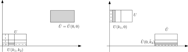
?figurename? 10: Two possibilities for the decomposition into subboxes

A simple but crucial observation is that since $I_{i}$ and $\tilde{I}_{i}$ are separated for both $i=1$ and $i=2$, we have $\mathcal{N}_{i}=\{0\}$ or $\tilde{\mathcal{N}}_{i}=\{0\}$ (cf. Figures 10). Hence for each pair $(k_{i},\tilde{k}_{i})\in\mathcal{N}_{i}\times\tilde{\mathcal{N}}_{i}$, $k_{i}=0$ or $\tilde{k}_{i}=0$, and thus

$$\bar{\kappa}_{i}(k_{i},\tilde{k}_{i}):=\max\{\kappa_{i}(k_{i}),\tilde{\kappa}_{i}(\tilde{k}_{i})\}=\max\{2^{-k_{i}(m_{i}-2)},2^{-\tilde{k}_{i}(m_{i}-2)}\}\varkappa_{i}=\varkappa_{i}$$ (5.4)

$$\bar{d}_{i}(k_{i},\tilde{k}_{i}):=\max\{d_{i}(k_{i}),\tilde{d}_{i}(\tilde{k}_{i})\}=\max\{2^{-k_{i}},2^{-\tilde{k}_{i}}\}\rho_{i}=\rho_{i}.$$ (5.5)

We conclude that

$$\frac{\kappa_{i}(k_{i})}{\bar{\kappa}_{i}(k_{i},\tilde{k}_{i})}=2^{-k_{i}(m_{i}-2)},$$ (5.6)

$$\frac{\tilde{\kappa}_{i}(k_{i})}{\bar{\kappa}_{i}(k_{i},\tilde{k}_{i})}=2^{-\tilde{k}_{i}(m_{i}-2)}\frac{d_{i}(k_{i})}{\bar{d}_{i}}=2^{-k_{i}},$$ (5.7)

$$d_{i}(k_{i})\tilde{d}_{i}(\tilde{k}_{i})=2^{-k_{i}-\tilde{k}_{i}}\rho_{i}^{2}=2^{-k_{i}\vee\tilde{k}_{i}}\rho_{i}^{2},$$ (5.8)

hence

$$Q= q(\bar{\kappa}_{1}\bar{d}_{1}^{2},\bar{\kappa}_{2}\bar{d}_{2}^{2})\prod_{i=1,2}q(d_{i}(k_{i}),\tilde{d}_{i}(\tilde{k}_{i}))q(\kappa_{i}(k_{i}),\tilde{\kappa}_{i}(\tilde{k}_{i}))$$

$$\leq \frac{\bar{\kappa}_{1}\bar{d}_{1}^{2}\vee\bar{\kappa}_{2}\bar{d}_{2}^{2}}{\bar{\kappa}_{1}\bar{d}_{1}^{2}\wedge\bar{\kappa}_{2}\bar{d}_{2}^{2}}2^{m_{1}(k_{1}+\tilde{k}_{1})+m_{2}(k_{2}+\tilde{k}_{2})}.$$ (5.9)

Thus, if we apply inequality (4.23) from Theorem 4.3 to the pairs of hypersurfaces $S(k),\tilde{S}(\tilde{k})$ and estimate by means of (5.4)–(Proof:), then we get

$$\|R^{*}_{S,\tilde{S}}\|_{L^{q}\times L^{q}\to L^{p}}\leq\sum_{k\in\mathcal{N},\tilde{k}\in\tilde{\mathcal{N}}}\|R^{*}_{S(k),\tilde{S}(\tilde{k})}\|_{L^{q}\times L^{q}\to L^{p}}$$

$$\lesssim(\varkappa_{1}\rho_{1}^{2}\varkappa_{2}\rho_{2}^{2})^{\frac{3}{p}-2+2\varepsilon}(\rho_{1}\rho_{2})^{\frac{2}{q^{\prime}}-\frac{1}{p}}\log^{\gamma}\left(\frac{\varkappa_{1}\rho_{1}^{2}}{\varkappa_{2}\rho_{2}^{2}}+\frac{\varkappa_{2}\rho_{2}^{2}}{\varkappa_{1}\rho_{1}^{2}}\right)\Big{(}\sum_{k\in\mathcal{N},\tilde{k}\in\tilde{\mathcal{N}}}[1+k_{1}+\tilde{k}_{1}+k_{2}+\tilde{k}_{2}]^{\gamma}$$

$$\times(\varkappa_{1}\rho_{1}^{2}2^{-k_{1}-\tilde{k}_{1}}\wedge\varkappa_{2}\rho_{2}^{2}2^{-k_{2}-\tilde{k}_{2}})^{3-3\varepsilon-\frac{5}{p}}\ 2^{-(k_{1}+\tilde{k}_{1}+k_{2}+\tilde{k}_{2})\left(\frac{1}{2}-\frac{1}{q}\right)}\Big{)}$$

$$\times\left(\varkappa_{1}\rho_{1}^{2}2^{-k_{2}(m_{2}-2)}\vee\varkappa_{2}\rho_{2}^{2}2^{-k_{1}(m_{1}-2)}\right)^{\frac{1-\varepsilon}{2}-\frac{1}{p}}\left(\varkappa_{1}\rho_{1}^{2}2^{-\tilde{k}_{2}(m_{2}-2)}\vee\varkappa_{2}\rho_{2}^{2}2^{-\tilde{k}_{1}(m_{1}-2)}\right)^{\frac{1-\varepsilon}{2}-\frac{1}{p}}.$$

We claim that

$$\sum_{k\in\mathcal{N},\tilde{k}\in\tilde{\mathcal{N}}}[1+k_{1}+\tilde{k}_{1}+k_{2}+\tilde{k}_{2}]^{\gamma}(\varkappa_{1}\rho_{1}^{2}2^{-k_{1}-\tilde{k}_{1}}\wedge\varkappa_{2}\rho_{2}^{2}2^{-k_{2}-\tilde{k}_{2}})^{3-3\varepsilon-\frac{5}{p}}$$

$$\hskip 28.45274pt\times 2^{-(k_{1}+\tilde{k}_{1}+k_{2}+\tilde{k}_{2})\left(\frac{1}{2}-\frac{1}{q}\right)}\left(\varkappa_{1}\rho_{1}^{2}2^{-k_{2}(m_{2}-2)}\vee\varkappa_{2}\rho_{2}^{2}2^{-k_{1}(m_{1}-2)}\right)^{\frac{1-\varepsilon}{2}-\frac{1}{p}}$$

$$\hskip 28.45274pt\times\left(\varkappa_{1}\rho_{1}^{2}2^{-\tilde{k}_{2}(m_{2}-2)}\vee\varkappa_{2}\rho_{2}^{2}2^{-\tilde{k}_{1}(m_{1}-2)}\right)^{\frac{1-\varepsilon}{2}-\frac{1}{p}}$$

$$\lesssim(\varkappa_{1}\rho_{1}^{2}\wedge\varkappa_{2}\rho_{2}^{2})^{3-3\varepsilon-\frac{5}{p}}(\varkappa_{1}\rho_{1}^{2}\vee\varkappa_{2}\rho_{2}^{2})^{1-\varepsilon-\frac{2}{p}}.$$ (5.10)

Taking this for granted, we arrived at estimate (5.1):

$$\|R^{*}_{S,\tilde{S}}\|_{L^{2}\times L^{2}\to L^{p}(Q_{S,\tilde{S}}(R))}\lesssim(\varkappa_{1}\rho_{1}^{2}\varkappa_{2}\rho_{2}^{2})^{\frac{3}{p}-2+2\varepsilon}(\rho_{1}\rho_{2})^{\frac{2}{q^{\prime}}-\frac{1}{p}}$$

$$\hskip 28.45274pt\times(\varkappa_{1}\rho_{1}^{2}\vee\varkappa_{2}\rho_{2}^{2})^{1-\varepsilon-\frac{2}{p}}(\varkappa_{1}\rho_{1}^{2}\wedge\varkappa_{2}\rho_{2}^{2})^{3-3\varepsilon-\frac{5}{p}}\log^{\gamma}\left(\frac{\varkappa_{1}\rho_{1}^{2}}{\varkappa_{2}\rho_{2}^{2}}+\frac{\varkappa_{2}\rho_{2}^{2}}{\varkappa_{1}\rho_{1}^{2}}\right)$$

$$=(\rho_{1}\rho_{2})^{\frac{2}{q^{\prime}}-\frac{1}{p}}(\varkappa_{1}\rho_{1}^{2}\vee\varkappa_{2}\rho_{2}^{2})^{\frac{1}{p}-1+\varepsilon}(\varkappa_{1}\rho_{1}^{2}\wedge\varkappa_{2}\rho_{2}^{2})^{1-\frac{2}{p}-\varepsilon}\log^{\gamma}\left(\frac{\varkappa_{1}\rho_{1}^{2}}{\varkappa_{2}\rho_{2}^{2}}+\frac{\varkappa_{2}\rho_{2}^{2}}{\varkappa_{1}\rho_{1}^{2}}\right).$$

We are thus left with the estimation of the dyadic sum in (5.10). Let

$$\mu=\frac{1}{p}-\frac{1-\varepsilon}{2}>0,\quad\nu=3-3\varepsilon-\frac{5}{p}>0,\quad\omega=\frac{1}{2}-\frac{1}{q}>0,\quad c_{i}=m_{i}-2.$$

Then $c_{i}\mu<\nu+\omega$ is equivalent to $m_{i}\left({1}/{p}-1/2\right)+\mathcal{O}(\varepsilon)<{1}/{q^{\prime}}$. This is satisfied since by our assumptions in the theorem we have $m_{i}\left({1}/{p}-{1}/{2}\right)<{1}/{q^{\prime}},$ and we can chose $\varepsilon$ arbitrarily small.

Estimate (5.10) will then be an easy consequence of the next lemma. Indeed, recalling our earlier observation that for each pair $(k_{i},\tilde{k}_{i})\in\mathcal{N}_{i}\times\tilde{\mathcal{N}}_{i}$ one of the entries $k_{i}$ or $\tilde{k}_{i}$ must be zero, we see that we have to sum over at most two of the parameters $k_{1},k_{2},\tilde{k}_{1},\tilde{k}_{2}$.

Thus, there are four possibilities: if exactly two of the parameters are nonzero, then there are two distinct cases: either these parameters belong to the same surface (i.e., $k_{1}=k_{2}=0$ or $\tilde{k}_{1}=\tilde{k}_{2}=0$), which correspond to the left picture in Figure 10, or the nonzero parameters belong to two different surfaces, as in the "over cross" situation shown in the picture on the right hand side of Figure 10. The remaining two possibilities are firstly that only one parameter $k_{1},k_{2},\tilde{k}_{1},\tilde{k}_{2}$ is nonzero, which happens if only one of the rectangles $U,\tilde{U}$ touches only one of the axes, and secondly the situation where both rectangles are located away from the axes. In this last situation, we have indeed no further decomposition and only one term to sum.

The first two of the afore-mentioned possibilities can be dealt with directly by the next lemma. But, notice that the corresponding sums of course dominate the sums over fewer parameters (or even none), which allows to also handle the remaining two possibilities. $\Box$

Lemma 5.2.

Let $\mu,\omega\geq 0$, $\nu>0$, $n,c_{1},c_{2}\geq 0$ such that $(c_{1}\vee c_{2})\mu<\nu+\omega$, and let $a,b\in\mathbbm{R}_{+}$. Then

$$\sum\limits_{k_{1},k_{2}\in\mathbbm{N}}(1+k_{1}+k_{2})^{n}2^{-(k_{1}+k_{2})\omega}(a2^{-k_{2}c_{2}}\vee b)^{-\mu}(a\vee b2^{-k_{1}c_{1}})^{-\mu}(a2^{-k_{1}}\wedge b2^{-k_{2}})^{\nu}$$

$$\leq \sum\limits_{k_{1},k_{2}\in\mathbbm{N}}(1+k_{1}+k_{2})^{n}2^{-(k_{1}+k_{2})\omega}(a\vee b)^{-\mu}(a2^{-k_{2}c_{2}}\vee b2^{-k_{1}c_{1}})^{-\mu}(a2^{-k_{1}}\wedge b2^{-k_{2}})^{\nu}$$

$$\lesssim (a\vee b)^{-2\mu}(a\wedge b)^{\nu}.$$

In the last estimate, the constant hidden by the symbol $\lesssim$ will depend only on the exponent $n$.

We remark that the bound in this lemma is essentially sharp, as one can immediately see by looking at the term with $k_{1}=0=k_{2}$. Notice that the proof is easier when $\omega>0$.

Proof:.

To prove the first inequality, observe that $a2^{-k_{2}c_{2}}\vee b2^{-k_{1}c_{1}}$ is bounded by $a2^{-k_{2}c_{2}}\vee b$ as well as by $a\vee b2^{-k_{1}c_{1}},$ hence by the minimum of these expressions. Therefore we have

$$(a2^{-k_{2}c_{2}}\vee b)\wedge(a\vee b2^{-k_{1}c_{1}}) \geq a2^{-k_{2}c_{2}}\vee b2^{-k_{1}c_{1}}$$

$$(a2^{-k_{2}c_{2}}\vee b)\vee(a\vee b2^{-k_{1}c_{1}}) =a\vee b,$$

hence

$$(a2^{-k_{2}c_{2}}\vee b)(a\vee b2^{-k_{1}c_{1}})\geq(a\vee b)(a2^{-k_{2}c_{2}}\vee b2^{-k_{1}c_{1}}).$$

Using the symmetry in this estimate, it suffices to estimate

$$S=a^{\nu}\sum_{\underset{a2^{-k_{1}}\leq b2^{-k_{2}}}{k_{1},k_{2}\in\mathbbm{N}}}k_{1}^{n}k_{2}^{n}2^{-(k_{1}+k_{2})\omega}(a2^{-k_{2}c_{2}}\vee b2^{-k_{1}c_{1}})^{-\mu}2^{-k_{1}\nu}.$$

On the one hand, we have

$$S\leq a^{\nu}b^{-\mu}\sum_{k_{1}}k_{1}^{n}2^{k_{1}(c_{1}\mu-\nu-\omega)}\sum\limits_{k_{2}:a2^{-k_{1}}\leq b2^{-k_{2}}}k_{2}^{n}2^{-k_{2}\omega}$$

$$\leq a^{\nu}b^{-\mu}\log^{n+1}\left(\frac{a}{b}+\frac{b}{a}\right)\sum_{k_{1}}k_{1}^{2n+1}2^{k_{1}(c_{1}\mu-\nu-\omega)}$$

$$\lesssim a^{\nu}b^{-\mu}\log^{n+1}\left(\frac{a}{b}+\frac{b}{a}\right).$$

In the case $\omega>0$, we might get along even without the $\log$-term. On the other hand,

$$S \leq a^{\nu-\mu}\sum_{k_{2}}k_{2}^{n}2^{k_{2}(c_{2}\mu-\omega)}\sum_{k_{1}:a2^{-k_{1}}\leq b2^{-k_{2}}}k_{1}^{n}2^{-k_{1}(\nu+\omega)}$$

$$\leq a^{\nu-\mu}\sum_{k_{2}}k_{2}^{n}2^{k_{2}(c_{2}\mu-\omega)}\sum_{k_{1}:a2^{-k_{1}}\leq b2^{-k_{2}}}k_{1}^{n}2^{-k_{1}\nu}$$

$$\sim a^{\nu-\mu}\log^{n}\left(\frac{a}{b}+\frac{b}{a}\right)\left(\frac{b}{a}\right)^{\nu}\sum_{k_{2}}k_{2}^{2n}2^{k_{2}(c_{2}\mu-\nu-\omega)}$$

$$\sim a^{-\mu}b^{\nu}\log^{n}\left(\frac{a}{b}+\frac{b}{a}\right).$$

Combining these two estimates, we obtain

$$\frac{S}{\log^{n+1}\left(\frac{a}{b}+\frac{b}{a}\right)}\lesssim a^{-\mu}b^{\nu}\wedge a^{\nu}b^{-\mu}=(a\vee b)^{-\mu}(a\wedge b)^{\nu}.$$

$\Box$

6 Passage from bilinear to linear estimates

Recall that $\bar{m}=m_{1}\vee m_{2},\,m=m_{1}\wedge m_{2}$ and ${1}/{h}={1}/{m_{1}}+{1}/{m_{2}}$. The first step to prove our main Theorem 1.2 is the following Lorentz space estimate for the adjoint restriction operator $R^{*}$ associated to $\Gamma=\text{\rm graph\,}(\phi).$

Theorem 6.1.

Let $p_{0}=1+{\bar{m}}/(\bar{m}+m)$, $2p>\max\{{10}/{3},2p_{0},h+1\}$ and ${1}/{s^{\prime}}\geq(h+1)/{2p}$. Then $R^{*}$ is bounded from $L^{s,t}(\Gamma,d\nu)$ to $L^{2p,t}(\mathbbm{R}^{3})$ for any $1\leq t\leq\infty$.

Proof:.

We begin by observing that we may assume that

$$\frac{h+1}{p}>1.$$ (6.1)

Indeed, if $2p\geq 2(h+1),$ then we have the Stein-Tomas type result that $R^{*}$ is bounded from $L^{2}(\Gamma,d\nu)$ to $L^{2p}(\mathbbm{R}^{3})$ (see [IKM10], [IM11]). Interpolating this with the trivial estimate from $L^{1}(\Gamma,d\nu)$ to $L^{\infty}(\mathbbm{R}^{3})$ and applying Hölder’s inequality on $\Gamma,$ we see that the situation where $(h+1)/p\leq 1$ is settled in Theorem 6.1.

In the remaining cases, interpolation theory for Lorentz spaces (see, e.g., [Gra08]) shows that it suffices to prove the restricted weak-type estimate

$$\|\widehat{\chi_{\Omega}d\nu}\|_{2p}\lesssim|\Omega|^{\frac{1}{s}}$$ (6.2)

for any measurable set $\Omega\subset Q=[0,1]\times[0,1]$.

To this end we perform the kind of Whitney decomposition mentioned in Section 5 of $Q\times Q=\bigcup\limits_{j}\bigcup\limits_{k\approx\tilde{k}}\tau_{jk}\times\tau_{j\tilde{k}}$ into “well-separated neighboring rectangles” $\tau_{jk}$ and $\tau_{j\tilde{k}},$ where

$$\tau_{jk}=[(k_{1}-1)2^{-j_{1}},k_{1}2^{-j_{1}}]\times[(k_{2}-1)2^{-j_{2}},k_{2}2^{-j_{2}}],$$

and where $k\approx\tilde{k}$ means that $2\leq|k_{i}-\tilde{k}_{i}|\leq C$, $i=1,2$ (compare [L05],[V05]). Then we may estimate

$$\|\widehat{\chi_{\Omega}d\nu}\|_{2p}^{2}=\|\widehat{\chi_{\Omega}d\nu}\widehat{\chi_{\Omega}d\nu}\|_{p}\leq\sum_{j}\big{[}\sum_{k\sim\tilde{k}}\|\textfrak{F}(\chi_{\Omega\cap\tau_{jk}}d\nu)\textfrak{F}(\chi_{\Omega\cap\tau_{j\tilde{k}}}d\nu)\|_{p}^{p^{*}}\big{]}^{\frac{1}{p^{*}}},$$

where

$$p^{*}=\min\{p,p^{\prime}\},$$ (6.3)

with ${1}/{p}+{1}/{p^{\prime}}=1$. The last step can be obtained by interpolation between the cases $p=2$, where one may apply Plancherel’s theorem, and the cases $p=1$ and $p=\infty,$ which are simply treated by means of the triangle inequality (compare Lemma 6.3. in [TVI00]). We claim that

$$(\bar{m}+3)\left(\frac{1}{p}-\frac{1}{2}\right)<\frac{h+1}{2p}.$$ (6.4)

Case 1: $\bar{m}\leq 2m.$ Then $\bar{m}\leq 3h$ and

$$(\bar{m}+3)\left(\frac{1}{p}-\frac{1}{2}\right)-\frac{h+1}{2p}\leq 3(h+1)\left(\frac{1}{p}-\frac{1}{2}\right)-\frac{h+1}{2p}=(h+1)\left(\frac{5}{2p}-\frac{3}{2}\right)<0$$

according to our assumptions.

Case 2: $\bar{m}>2m.$ Here,

$$h+1=\frac{\bar{m}m+\bar{m}+m}{\bar{m}+m}>\frac{\bar{m}m+3m}{\bar{m}+m}=(\bar{m}+3)\frac{m}{\bar{m}+m},$$

and thus

$$(\bar{m}+3)\left(\frac{1}{p}-\frac{1}{2}\right)-\frac{h+1}{2p}<(\bar{m}+3)\left(\frac{1}{p}-\frac{1}{2}-\frac{m}{\bar{m}+m}\frac{1}{2p}\right)$$

$$=(\bar{m}+3)\left(\frac{1}{2p}\left(1+\frac{\bar{m}}{\bar{m}+m}\right)-\frac{1}{2}\right)<0,$$

because of our assumption $2p>2p_{0}$.

In both cases, these estimates show that we may choose $q\geq 2$ such that

$$(\bar{m}+3)\left(\frac{1}{p}-\frac{1}{2}\right)<\frac{1}{q^{\prime}}<\frac{h+1}{2p}$$ (6.5)

(recall here (6.1), which allows to choose $q\geq 2$).

The first inequality allows to apply Theorem 5.1 to the pair of hypersurfaces $S_{jk}=\{(\xi,\phi(\xi)):\xi\in\tau_{jk}\}$ and $S_{j\tilde{k}}=\{(\xi,\phi(\xi)):\xi\in\tau_{j\tilde{k}}\},$ with

$$\rho_{i}= 2^{-j_{i}}$$

$$\varkappa_{i}\sim (k_{i}2^{-j_{i}})^{m_{i}-2}\sim(\tilde{k}_{i}2^{-j_{i}})^{m_{i}-2}$$ (6.6)

$$\varkappa_{i}\rho_{i}^{2}\sim k_{i}^{m_{i}-2}2^{-j_{i}m_{i}}.$$

Without loss of generality, we may assume that

$$k\in I:=\{k|k_{1}^{m_{1}-2}2^{-j_{1}m_{1}}\geq k_{2}^{m_{2}-2}2^{-j_{2}m_{2}}\},$$ (6.7)

i.e., $\varkappa_{1}\rho_{1}^{2}\geq\varkappa_{2}\rho_{2}^{2}$. Thus, by Theorem 5.1,

$$\|R^{*}_{S_{jk},S_{j\tilde{k}}}\|_{L^{q}(S_{jk})\times L^{q}(S_{j\tilde{k}})\to L^{p}(\mathbbm{R}^{3})}$$

$$\lesssim (\rho_{1}\rho_{2})^{\frac{2}{q^{\prime}}-\frac{1}{p}}(\varkappa_{1}\rho^{2}_{1}\vee\varkappa_{2}\rho^{2}_{2})^{-\frac{1}{p}}\left(\frac{\varkappa_{1}\rho^{2}_{1}\vee\varkappa_{2}\rho^{2}_{2}}{\varkappa_{1}\rho^{2}_{1}\wedge\varkappa_{2}\rho^{2}_{2}}\right)^{\frac{2}{p}-1+\varepsilon}$$

$$= 2^{-(j_{1}+j_{2})\left(\frac{2}{q^{\prime}}-\frac{1}{p}\right)}k_{1}^{-(m_{1}-2)\frac{1}{p}}2^{j_{1}m_{1}\frac{1}{p}}\left(\frac{k_{1}^{m_{1}-2}}{k_{2}^{m_{2}-2}}2^{-(j_{1}m_{1}-j_{2}m_{2})}\right)^{\frac{2}{p}-1+\varepsilon}$$

$$= A_{j}\cdot B_{k,j}^{\frac{1}{p}},$$

if we define

$$A_{j}=2^{-(j_{1}+j_{2})\left(\frac{2}{q^{\prime}}-\frac{1}{p}\right)}2^{j_{1}m_{1}\frac{1}{p}}2^{-(j_{1}m_{1}-j_{2}m_{2})\frac{2}{p}-1+\varepsilon},$$

$$B_{j,\tilde{k}}\sim B_{k,j}=k_{1}^{-(m_{1}-2)}\left(\frac{k_{1}^{m_{1}-2}}{k_{2}^{m_{2}-2}}\right)^{2-p+\varepsilon p}.$$

Since $|\{\tilde{k}:k\sim\tilde{k}\}|\lesssim 1$ for fixed $k$, we conclude that

$$\|\widehat{\chi_{\Omega}d\nu}\|_{2p}^{2} \lesssim \sum_{j}A_{j}\left[\sum_{k\sim\tilde{k}}\left(B_{k,j}^{\frac{1}{p}}|\Omega\cap\tau_{jk}|^{\frac{1}{q}}|\Omega\cap\tau_{j\tilde{k}}|^{\frac{1}{q}}\right)^{p^{*}}\right]^{\frac{1}{p^{*}}}$$

$$\lesssim \sum_{j}A_{j}\left[\sum_{k}B_{k,j}^{\frac{p^{*}}{p}}|\Omega\cap\tau_{jk}|^{\frac{2p^{*}}{q}}\right]^{\frac{1}{p^{*}}}.$$

Therefore we are reduced to showing that

$$\sum_{j}A_{j}\left[\sum_{k}B_{k,j}^{\frac{p^{*}}{p}}|\Omega\cap\tau_{jk}|^{\frac{2p^{*}}{q}}\right]^{\frac{1}{p^{*}}}\lesssim |\Omega|^{\frac{2}{s}}.$$ (6.8)

6.1 Further reduction

We decompose

$$\frac{2p^{*}}{q}=\frac{\alpha}{r^{*}}+\frac{1}{{r^{*}}^{\prime}},$$

where $r*\in[1,\infty]$ will be determined later, and introduce $r={r^{*}p^{*}}/{p}$. Applying Hölder’s inequality to the summation in $k,$ with Hölder exponent $r^{*}\geq 1,$ we get

$$\left(\sum_{k\in I}B_{k,j}^{\frac{p^{*}}{p}}|\Omega\cap\tau_{jk}|^{\frac{2p^{*}}{q}}\right)^{\frac{1}{p^{*}}} \leq \left(\sum_{k\in I}B_{k,j}^{\frac{p^{*}r^{*}}{p}}|\Omega\cap\tau_{jk}|^{\alpha}\right)^{\frac{1}{p^{*}r^{*}}}\leavevmode\nobreak\ \left(\sum_{k\in I}|\Omega\cap\tau_{jk}|\right)^{\frac{1}{p^{*}{r^{*}}^{\prime}}}$$

$$\leq \left(\sum_{k\in I}B_{k,j}^{r}\right)^{\frac{1}{pr}}\leavevmode\nobreak\ \min\{|\Omega|,2^{-j_{1}-j_{2}}\}^{\frac{\alpha}{p^{*}r^{*}}}\leavevmode\nobreak\ |\Omega|^{\frac{1}{p^{*}}\left(1-\frac{1}{r^{*}}\right)}$$

$$= \left(\sum_{k\in I}B_{k,j}^{r}\right)^{\frac{1}{pr}}\leavevmode\nobreak\ \min\{|\Omega|,2^{-j_{1}-j_{2}}\}^{\frac{2}{q}-\frac{1}{p^{*}}+\frac{1}{pr}}\leavevmode\nobreak\ |\Omega|^{\frac{1}{p^{*}}-\frac{1}{pr}}.$$

Moreover we have $|\Omega|\leq|Q|=1,$ as well as $1/{s^{\prime}}\geq{h+1}/{2p}$, i.e., $2-(h+1)/{p}\geq{2}/{s}$. Therefore $|\Omega|^{2-\frac{h+1}{p}}\leq|\Omega|^{\frac{2}{s}}$, and thus in order to prove (6.8), it suffices to show that

$$|\Omega|^{2-\frac{h+1}{p}-\frac{1}{p^{*}}+\frac{1}{pr}}\gtrsim\sum_{j}A_{j}\min\{|\Omega|,2^{-j_{1}-j_{2}}\}^{\frac{2}{q}-\frac{1}{p^{*}}+\frac{1}{pr}}\left[\sum_{k\in I}B_{k,j}^{r}\right]^{\frac{1}{rp}},$$

i.e., that

$$|\Omega|^{2-\frac{h+1}{p}-\frac{1}{p^{*}}+\frac{1}{pr}}$$

$$\gtrsim\sum_{j}2^{-(j_{1}m_{1}-j_{2}m_{2})\frac{2}{p}-1+\varepsilon}2^{-(j_{1}+j_{2})\left(\frac{2}{q^{\prime}}-\frac{1}{p}\right)}2^{j_{1}m_{1}\frac{1}{p}}\min\{|\Omega|,2^{-j_{1}-j_{2}}\}^{\frac{2}{q}-\frac{1}{p^{*}}+\frac{1}{pr}}$$

$$\hskip 56.9055pt\times\left[\sum_{k\in I}k_{1}^{(m_{1}-2)(1-p+\varepsilon p)r}k_{2}^{(m_{2}-2)(p-2-\varepsilon p)r}\right]^{\frac{1}{pr}}.$$

We apply the change of variables $l=j_{1}+j_{2}\in\mathbbm{N}$, $l^{\prime}=j_{1}m_{1}-j_{2}m_{2}\in\mathbbm{Z}$, such that

$$j_{1}=\frac{m_{2}l+l^{\prime}}{m_{1}+m_{2}}.$$

Then the exponent in $j_{1},j_{2}$ becomes

$$(j_{1}m_{1}-j_{2}m_{2})\left(1-\frac{2}{p}-\varepsilon\right)+(j_{1}+j_{2})\left(\frac{1}{p}-\frac{2}{q^{\prime}}\right)+j_{1}m_{1}\frac{1}{p}$$

$$= l^{\prime}\left(1-\frac{2}{p}-\varepsilon\right)+l\left(\frac{1}{p}-\frac{2}{q^{\prime}}\right)+\frac{m_{1}m_{2}l+m_{1}l^{\prime}}{m_{1}+m_{2}}\frac{1}{p}$$

$$= \frac{l^{\prime}}{p}\left(p-\varepsilon p-\frac{m_{1}+2m_{2}}{m_{1}+m_{2}}\right)+l\left(\frac{h+1}{p}-\frac{2}{q^{\prime}}\right).$$

The summation over $k\in I_{l^{\prime}}=\{k_{1}^{m_{1}-2}\geq k_{2}^{m_{2}-2}2^{l^{\prime}}\}$ is independent of $l$, and thus we have finally reduced the proof of (6.8) to proving the following two decoupled estimates:

$$\sum_{l^{\prime}=-\infty}^{\infty}2^{\frac{l^{\prime}}{p}(p-\varepsilon p-\frac{m_{1}+2m_{2}}{m_{1}+m_{2}})}\left[\sum_{k\in I_{l^{\prime}}}k_{1}^{(m_{1}-2)(1-p+\varepsilon p)r}k_{2}^{(m_{2}-2)(p-2-\varepsilon p)r}\right]^{\frac{1}{pr}}<\infty$$ (6.9)

and

$$\sum_{l=0}^{\infty}2^{l(\frac{h+1}{p}-\frac{2}{q^{\prime}})}\min\{|\Omega|,2^{-l}\}^{\frac{2}{q}-\frac{1}{p^{*}}+\frac{1}{pr}}\lesssim|\Omega|^{2-\frac{h+1}{p}-\frac{1}{p^{*}}+\frac{1}{pr}}.$$ (6.10)

6.2 The case $m>2$

In this case we have both $m_{1}>2$ and $m_{2}>2$.

6.2.1 Summation in $k$

We compare the sum over $k$ in (6.9) with an integral. We claim that

$$\int\limits_{\underset{k_{1}^{m_{1}-2}\geq k_{2}^{m_{2}-2}2^{l^{\prime}}}{k_{1},k_{2}\geq 1}}k_{1}^{(m_{1}-2)(1-p+\varepsilon p)r}k_{2}^{(m_{2}-2)(p-\varepsilon p-2)r}dk$$

$$\hskip 42.67912pt\lesssim\begin{cases}2^{|l^{\prime}|(\frac{1}{m_{1}-2}+(1-p+\varepsilon p)r)},&l^{\prime}\geq 0\\ |l^{\prime}|2^{|l^{\prime}|(\frac{1}{m_{2}-2}+(p-\varepsilon p-2)r)_{+}},&l^{\prime}<0,\end{cases},$$ (6.11)

provided that

$$a:=\frac{1}{m_{1}-2}+(1-p+\varepsilon p)r<0$$ (6.12)

and

$$a+b=\frac{1}{m_{1}-2}+\frac{1}{m_{2}-2}-r<0,$$ (6.13)

where

$$b :=\frac{1}{m_{2}-2}+(p-\varepsilon p-2)r\in\mathbbm{R}.$$ (6.14)

For the moment, we will simply assume that these conditions hold true. We shall collect several further conditions on the exponent $r$ and verify at the end of this section that we can indeed find an $r$ such that all these conditions are satisfied.

By means of the coordinate transformation $s=k_{1}^{m_{1}-2}$, $t=k_{2}^{m_{2}-2}$ (i.e., $dk\sim s^{\frac{1}{m_{1}-2}-1}t^{\frac{1}{m_{2}-2}-1}d(s,t)$ ), (6.2.1) simplifies to showing that

$$J(a,b)=\underset{\underset{\scriptstyle s\geq t2^{l^{\prime}}}{s,t\geq 1}}{\int\int}s^{a}t^{b}\frac{ds}{s}\frac{dt}{t}\lesssim\begin{cases}2^{|l^{\prime}|a}&l^{\prime}\geq 0\\ 2^{|l^{\prime}|b_{+}}&l^{\prime}<0,\end{cases},$$ (6.15)

provided that $a<0$, $a+b<0$. Here we have set $b_{+}=b\vee 0.$ Changing $t^{\prime}=s2^{-l^{\prime}}/t$, the set of integration for the $t$-variable $\{t:t\geq 1,s2^{-l^{\prime}}/t\geq 1\}$ transforms into $\{t^{\prime}:s2^{-l^{\prime}}/t^{\prime}\geq 1,t^{\prime}\geq 1\},$ and thus, since we assume that $a+b<0,$

$$J(a,b) = \underset{\underset{\scriptstyle s\geq t^{\prime}2^{l^{\prime}}}{s,t^{\prime}\geq 1}}{\int\int}s^{a}\left(\frac{s}{t^{\prime}}2^{-l^{\prime}}\right)^{b}\frac{ds}{s}\frac{dt^{\prime}}{t^{\prime}}=2^{-l^{\prime}b}\int_{t^{\prime}=1}^{\infty}t^{\prime-b}\int_{s=1\vee t^{\prime}2^{l^{\prime}}}^{\infty}s^{a+b}\frac{ds}{s}\frac{dt^{\prime}}{t^{\prime}}$$

$$= 2^{-l^{\prime}b}\int_{1}^{\infty}(1\vee t^{\prime}2^{l^{\prime}})^{a+b}t^{\prime-b}\frac{dt^{\prime}}{t^{\prime}}.$$

If $l^{\prime}\geq 0,$ then clearly $1\vee t^{\prime}2^{l^{\prime}}=t^{\prime}2^{l^{\prime}}$, and since $a<0,$ we get

$$J(a,b)=2^{l^{\prime}a}\int_{1}^{\infty}t^{\prime a}\frac{dt^{\prime}}{t^{\prime}}\sim 2^{l^{\prime}a}.$$

And, if $l^{\prime}<0$, the we split into

$$J(a,b)= 2^{-l^{\prime}b}\int_{1}^{2^{|l^{\prime}|}}t^{\prime-b}\frac{dt^{\prime}}{t^{\prime}}+2^{l^{\prime}a}\int_{2^{|l^{\prime}|}}^{\infty}t^{\prime a}\frac{dt^{\prime}}{t^{\prime}}=2^{-l^{\prime}b}\frac{1-2^{l^{\prime}b}}{b}+\int_{1}^{\infty}u^{a}\frac{du}{u}$$

$$\lesssim |l^{\prime}|(2^{|l^{\prime}|b}+1)\sim|l^{\prime}|2^{|l^{\prime}|b_{+}}$$

(notice that the additional factor $|l^{\prime}|$ arises in fact only when $b=0$). This proves (6.15).

6.2.2 Summation in $l^{\prime}$

In order to apply (6.2.1) to (6.9), we split the sum in (6.9) into summation over $l^{\prime}\geq 0$ and summation over $l^{\prime}<0$. In the first case $l^{\prime}\geq 0$, we obtain

$$\sum_{l^{\prime}\geq 0}2^{\frac{l^{\prime}}{p}(p-\varepsilon p-\frac{m_{1}+2m_{2}}{m_{1}+m_{2}})}\left[\sum_{k\in I}k_{1}^{(m_{1}-2)(1-p+\varepsilon p)r}k_{2}^{(m_{2}-2)(p-\varepsilon p-2)r}\right]^{\frac{1}{rp}}$$

$$\lesssim \sum_{l^{\prime}\geq 0}2^{\frac{l^{\prime}}{p}(p-\varepsilon p-1-\frac{m_{2}}{m_{1}+m_{2}})}2^{l^{\prime}(\frac{1}{pr}\frac{1}{m_{1}-2}+\frac{1-p+\varepsilon p}{p})}$$ (6.16)

$$= \sum_{l^{\prime}\geq 0}2^{\frac{l^{\prime}}{p}(\frac{1}{r}\frac{1}{m_{1}-2}-\frac{m_{2}}{m_{1}+m_{2}})}.$$

The sum is finite provided

$$\frac{1}{r}<\frac{m_{2}(m_{1}-2)}{m_{1}+m_{2}},$$ (6.17)

which gives yet another condition for our collection.

In the second case $l^{\prime}<0$, we have

$$\sum_{l^{\prime}<0}2^{\frac{l^{\prime}}{p}(p-\varepsilon p-\frac{m_{1}+2m_{2}}{m_{1}+m_{2}})}\left[\sum_{k\in I}k_{1}^{(m_{1}-2)(1-p+\varepsilon p)r}k_{2}^{(m_{2}-2)(p-\varepsilon p-2)r}\right]^{\frac{1}{rp}}$$

$$\lesssim \sum_{l^{\prime}<0}2^{\frac{l^{\prime}}{p}(p-\varepsilon p-\frac{m_{1}+2m_{2}}{m_{1}+m_{2}})}|l^{\prime}|2^{|l^{\prime}|(\frac{1}{pr}\frac{1}{m_{2}-2}+\frac{p-\varepsilon p-2}{p})_{+}}$$ (6.18)

$$= \sum_{l^{\prime}<0}|l^{\prime}|2^{\frac{l^{\prime}}{p}(p-\varepsilon p-\frac{m_{1}+2m_{2}}{m_{1}+m_{2}}-(\frac{1}{r}\frac{1}{m_{2}-2}+p-\varepsilon p-2)_{+})}.$$

Notice that for sufficiently small $\varepsilon>0$ we have $p-\varepsilon p>p_{0}=1+{\bar{m}}/(\bar{m}+m)\geq 1+{m_{2}}/(m_{1}+m_{2})$, and therefore

$$p-\varepsilon p-\frac{m_{1}+2m_{2}}{m_{1}+m_{2}}>0.$$ (6.19)

Thus the last sum in (6.2.2) converges in the case where

$$\frac{b}{r}=\frac{1}{r}\frac{1}{m_{2}-2}+p-\varepsilon p-2\leq 0.$$

This shows that we only need to discuss the case where $b>0$, in which we need that

$$0< p-\varepsilon p-\frac{m_{1}+2m_{2}}{m_{1}+m_{2}}-\frac{1}{r}\frac{1}{m_{2}-2}-p+\varepsilon p+2$$

$$= \frac{m_{1}}{m_{1}+m_{2}}-\frac{1}{r}\frac{1}{m_{2}-2},$$

which is equivalent to

$$\frac{1}{r}<\frac{m_{1}(m_{2}-2)}{m_{1}+m_{2}}.$$ (6.20)

Notice that this is of the same form as (6.17), only with the roles of $m_{1}$ and $m_{2}$ interchanged.

6.2.3 Summation in $l$

Recall that we want to show estimate (6.10), i.e.,

$$\sum_{l=0}^{\infty}2^{l(\frac{h+1}{p}-\frac{2}{q^{\prime}})}\min\{2^{-l},|\Omega|\}^{\frac{2}{q}-\frac{1}{p^{*}}+\frac{1}{pr}}\lesssim|\Omega|^{2-\frac{h+1}{p}-\frac{1}{p^{*}}+\frac{1}{pr}}.$$

We claim that it is sufficient to show that for $\mu>0$ and $\nu-\mu>0$

$$\int_{0}^{\infty}e^{x\mu}\min\{e^{-x},A\}^{\nu}dx\lesssim A^{\nu-\mu}.$$ (6.21)

Indeed, given (6.21), we apply it with $A=|\Omega|$, $\mu=(h+1)/p-2/{q^{\prime}}$ and $\nu={2}/{q}-{1}/{p^{*}}+1/{pr}$. Due to the choice of $q$ in (6.5), we have $\mu>0$. Moreover we want that

$$0<\nu-\mu=2-\frac{1}{p^{*}}+\frac{1}{pr}-\frac{h+1}{p}=\frac{1}{p}\left(2p-h-1-\frac{p}{p*}+\frac{1}{r}\right).$$

Notice that if $p\leq 2$, then ${p}/{p*}=1$, but if $p>2$, then ${p}/{p*}=p\left(1-{1}/{p}\right)=p-1$. Thus ${p}/{p*}=1+(p-2)_{+}$ for all $1\leq p\leq\infty$, i.e., the condition which is required here is

$$\frac{1}{r}>h+2-2p+(p-2)_{+}.$$ (6.22)

In order to verify (6.21), observe that

$$\int_{0}^{\infty}e^{x\mu}\min\{e^{-x},A\}^{\nu}dx= \int_{\ln A}^{\infty}e^{y\mu}A^{-\mu}\min\{e^{-y}A,A\}^{\nu}dy$$

$$= A^{\nu-\mu}\int_{\ln A}^{\infty}e^{y\mu}\min\{e^{-y},1\}^{\nu}dy.$$

The last integral can be estimated by

$$\int_{\ln A}^{\infty}e^{y\mu}\min\{e^{-y},1\}^{\nu}dy\leq\int_{-\infty}^{0}e^{y\mu}dy+\int_{0}^{\infty}e^{-y(\nu-\mu)}dy,$$

which is convergent since $\mu>0$ and $\nu-\mu>0$.

It still remains to be checked whether there exists some $1\leq r^{*}<\infty$ (for m>2) for which $r$ satisfies the conditions (6.12), (6.13), (6.17), (6.20) and (6.22).

This task will be accomplished in Lemma 6.2. First, we discuss the situation where $m=2$.

6.3 The case $m=2$

We will just give some hints how to modify the previous proof for this situation. In this case, $r=\infty$ turns out to be an appropriate choice, and the inequality that we need to start the argument with here reads

$$\left(\sum_{k\in I}B_{k,j}^{\frac{p^{*}}{p}}|\Omega\cap\tau_{jk}|^{\frac{2p^{*}}{q}}\right)^{\frac{1}{p^{*}}}\leq\big{(}\sup_{k\in I}B_{k,j}\big{)}^{\frac{1}{p}}\min\{|\Omega|,2^{-j_{1}-j_{2}}\}^{\frac{2}{q}-\frac{1}{p^{*}}}\leavevmode\nobreak\ |\Omega|^{\frac{1}{p^{*}}}.$$

This is very easy to prove, provided ${2p^{*}}/{q}\geq 1$ (notice that this condition corresponds to our previous decomposition of ${2p^{*}}/{q}$ when $r=\infty)$. To see that indeed ${2p^{*}}/{q}\geq 1,$ recall from (6.5) that $1/{q^{\prime}}<(h+1)/{2p}.$ Then, it is enough to check that $2p^{*}\left(1-(h+1)/{2p}\right)>1,$ i.e., $h+1-2p+p/{p^{*}}<0.$ The last condition is equivalent to $h+2-2p+(p-2)_{+}<0.$ However, this is what we shall indeed verify in the proof of Lemma 6.2 (compare estimate (6.30) when $m=2$).

Observe next that we may re-write the integral in $\eqref{sumink}$ in terms of the $L^{r}$-norm as

$$\left\|\left(k_{1}^{(m_{1}-2)(1-p+\varepsilon p)}k_{2}^{(m_{2}-2)(p-\varepsilon p-2)},\right)_{k\in I_{l^{\prime}}}\right\|_{r}\lesssim\begin{cases}2^{|l^{\prime}|(\frac{1}{r}\frac{1}{m_{1}-2}+1-p+\varepsilon p)}&l^{\prime}\geq 0,\\ |2^{|l^{\prime}|(\frac{1}{r}\frac{1}{m_{2}-2}+p-\varepsilon p-2)_{+}},&l^{\prime}<0,\end{cases}$$

provided the conditions (6.12) and (6.13) hold true, i.e., that

$$\frac{1}{m_{1}-2}+(1-p+\varepsilon p)r<0\quad\mbox{and}\quad\frac{1}{m_{1}-2}+\frac{1}{m_{2}-2}-r<0.$$

This gives rise to the conjecture that (for $r=\infty$) we should have

$$\sup_{k\in I}k_{1}^{(m_{1}-2)(1-p+\varepsilon p)} k_{2}^{(m_{2}-2)(p-\varepsilon p-2)}$$ (6.23)

$$\leq\sup_{s\geq t2^{l^{\prime}}}s^{1-p+\varepsilon p}t^{p-\varepsilon p-2} \lesssim\ \begin{cases}2^{|l^{\prime}|(1-p+\varepsilon p)}&l^{\prime}\geq 0\\ 2^{|l^{\prime}|(p-\varepsilon p-2)_{+}}&l^{\prime}<0,\end{cases}$$

which would suffice in this case. But notice that the conditions (6.12) and (6.13) are formally fulfilled for $r=\infty,$ and it is then easy to check that (6.23) indeed holds true, even in the case $m=2.$

6.3.1 Summation in $l^{\prime}$

The summation in $l^{\prime}$ becomes simpler here. We split again into the sums over $l^{\prime}\geq 0$ and $l^{\prime}<0$, and obtain for the first half of the sum in (6.2.2)

$$\sum_{l^{\prime}\geq 0}2^{\frac{l^{\prime}}{p}(p-\varepsilon p-\frac{m_{1}+2m_{2}}{m_{1}+m_{2}})}2^{l^{\prime}\frac{1-p+\varepsilon p}{p}}=\sum_{l^{\prime}\geq 0}2^{-\frac{l^{\prime}}{p}\frac{m_{2}}{m_{1}+m_{2}}}<\infty.$$

The second part of the sum becomes (compare (6.2.2))

$$\sum_{l^{\prime}<0}2^{\frac{l^{\prime}}{p}(p-\varepsilon p-\frac{m_{1}+2m_{2}}{m_{1}+m_{2}}-(p-\varepsilon p-2)_{+})}.$$

We already know from (6.19) that $p-\varepsilon p-(m_{1}+2m_{2})/(m_{1}+m_{2})>0$. Thus the sum converges if $p-\varepsilon p\leq 2$. For $p-\varepsilon p>2$, notice that

$$p-\varepsilon p-\frac{m_{1}+2m_{2}}{m_{1}+m_{2}}-(p-\varepsilon p-2)_{+}=\frac{m_{1}}{m_{1}+m_{2}}>0,$$

and thus the sum is finite.

6.3.2 Summation in $l$

It remains to show that

$$\qquad\sum_{l=0}^{\infty}2^{l(\frac{h+1}{p}-\frac{1}{q^{\prime}})}\min\{|\Omega|,2^{-l}\}^{\frac{1}{q}-\frac{1}{p^{*}}}\lesssim|\Omega|^{2-\frac{h+1}{p}-\frac{1}{p^{*}}},$$

which is the special case $r=\infty$ of (6.10). We saw that this holds true provided (6.22) is valid, i.e., if $1/{r}>h+2-2p+(p-2)_{+}$.

However, if $m=2,$ the

$$2p>p_{0}=\frac{2\bar{m}}{\bar{m}+2}+2=h+2.$$

Thus for the case $p\leq 2$ we have $h+2-2p+(p-2)_{+}=h+2-2p<0$. For the case $p>2$ notice that

$$h+2-2p+(p-2)_{+}=h-p=\frac{2\bar{m}}{\bar{m}+2}-p<2-p<0.$$

$\Box$

6.4 Final considerations

We finally verify that there is indeed always some $r$ for which all necessary conditions (6.12), (6.13), (6.17), (6.20) and (6.22) are satisfied in the case $m>2$. Recall that

$$\frac{2p^{*}}{q}=\frac{\alpha}{r^{*}}+\frac{1}{{r^{*}}^{\prime}},$$

and notice that it will suffice to verify the following equivalent inequalities:

$$\frac{1}{r}<(m_{1}-2)(p-1),$$ (6.24)

$$\frac{1}{r}<\frac{(m_{1}-2)(m_{2}-2)}{m_{1}+m_{2}-4},$$ (6.25)

$$\frac{1}{r}<\frac{m_{2}(m_{1}-2)}{m_{1}+m_{2}},$$ (6.26)

$$\frac{1}{r}<\frac{m_{1}(m_{2}-2)}{m_{1}+m_{2}},$$ (6.27)

$$\frac{1}{r}>h+2-2p+(p-2)_{+}.$$ (6.28)

Lemma 6.2.

Assume that $m>2$ and $2p>\max\{2p_{0},h+1\},$ where we recall that $p_{0}=1+{\bar{m}}/(\bar{m}+m).$ Define

$$J=\Big{]}0,1+(p-2)_{+}\Big{]}\cap\Big{]}h+2-2p+(p-2)_{+},\frac{\bar{m}(m-2)}{\bar{m}+m}\Big{[}.$$

Then $J\neq\emptyset,$ and for every $1/{r}\in J$ we have

$$r^{*}=\frac{rp}{p^{*}}\geq 1,\quad\mbox{and}\quad\alpha=r^{*}\left(\frac{2p^{*}}{q}-\frac{1}{{r^{*}}^{\prime}}\right)>0,$$ (6.29)

and moreover the inequalities (6.24), (6.25), (6.26), (6.27) and (6.28) are valid.

Proof:.

First of all, we will show that $J\neq\emptyset$. We need to see that

$$h+2-2p+(p-2)_{+}<\frac{\bar{m}(m-2)}{\bar{m}+m}=h-\frac{2\bar{m}}{\bar{m}+m},$$ (6.30)

i.e., that $2p_{0}=2+2\bar{m}/{\bar{m}+m}<2p-(p-2)_{+}$. For the case $p\leq 2$, this holds true since $2p>2p_{0}$. If $p>2$, observe that

$$h+2-2p+(p-2)_{+}=h-p<h-2\leq h-\frac{2\bar{m}}{\bar{m}+m}=\frac{\bar{m}(m-2)}{\bar{m}+m}.$$

Thus both intervals used for the definition of $J$ are not empty, but we still have to check that their intersection is not trivial. Since we assume that $2p>h+1$, we have

$$h+2-2p+(p-2)_{+}<1+(p-2)_{+}.$$

And, for $m>2$, we also have $0<\bar{m}(m-2)/(\bar{m}+m)$, which shows that $J\neq\emptyset$.

Next, if $1/{r}\in J$, then in particular ${1}/{r}\leq 1+(p-2)_{+}={p}/{p^{*}},$ and thus $r^{*}=r{p}/{p^{*}}\geq 1$. To prove (6.29), observe that due to our choice of $q$ in (6.5) we have $1/{q}>1-(h+1)/{2p}$, and thus it suffices to prove that

$$2p^{*}\left(1-\frac{h+1}{2p}\right)>\frac{1}{{r^{*}}^{\prime}}=1-\frac{p^{*}}{rp}.$$

This inequality is equivalent to

$$\frac{1}{r}>\frac{p}{p*}+h+1-2p=h+2-2p+(p-2)_{+},$$

and thus satisfied.

Considering the remaining conditions listed before the statement of the lemma, notice that (6.28) is immediate by the definition of $J$. Furthermore we have

$$\frac{1}{r}<\frac{\bar{m}(m-2)}{\bar{m}+m}=\frac{m_{1}m_{2}-2\bar{m}}{m_{1}+m_{2}}\leq\frac{m_{1}m_{2}-2m_{i}}{m_{1}+m_{2}}$$

for both $i=1,2$, which gives (6.26) and (6.27). To obtain (6.24), we estimate

$$\frac{1}{r}<\frac{\bar{m}(m-2)}{\bar{m}+m}\leq\frac{\bar{m}(m_{1}-2)}{\bar{m}+m}=(p_{0}-1)(m_{1}-2)<(p-\varepsilon p-1)(m_{1}-2).$$

Finally, observe that the following inequalities are all equivalent:

$$\frac{\bar{m}(m-2)}{\bar{m}+m} \leq\frac{(m_{1}-2)(m_{2}-2)}{m_{1}+m_{2}-4},$$

$$\frac{\bar{m}}{\bar{m}+m} \leq\frac{\bar{m}-2}{\bar{m}+m-4},$$

$$\bar{m}(\bar{m}+m)-4\bar{m} \leq\bar{m}(\bar{m}+m)-2(\bar{m}+m),$$

$$m \leq\bar{m}.$$

Hence (6.25) holds true as well. $\Box$

6.5 Finishing the proof

We can now conclude the prove of our main result, Theorem 1.2:

Corollary 6.3.

Let $2p>\max\{{10}/{3},h+1\}$, ${1}/{s^{\prime}}\geq(h+1)/{2p}$ and $1/{s}+(2\bar{m}+1)/{2p}<(\bar{m}+2)/{2}$. Then $R^{*}$ is bounded from $L^{s,t}(\Gamma)$ to $L^{2p,t}(\mathbbm{R}^{3})$ for every $1\leq t\leq\infty$. If moreover $s\leq 2p$ or $1/{s^{\prime}}>(h+1)/{2p}$, then $R^{*}$ is bounded from $L^{s}(\Gamma)$ to $L^{2p}(\mathbbm{R}^{3})$.

Proof:.

The crucial observation is that the intersection point of the two lines

$$\frac{1}{s^{\prime}}=\frac{h+1}{2p}\quad\mbox{and}\quad\frac{2\bar{m}+1}{2p}+\frac{1}{s}=\frac{\bar{m}+2}{2}$$

has the $p$-coordinate $p=\widehat{p_{0}}=1+{\bar{m}}/(\bar{m}+m)$ (comparing with (1.6), notice that $\widehat{p_{0}}=p_{0}/2$). So, what remains is to establish estimates for $R^{*}$ for the missing points $(1/s,1/p)$ lying within the sectorial region defined by the conditions $(2\bar{m}+1)/{2p}+1/{s}<(\bar{m}+2)/{2}$ and $1/p>1/\widehat{p_{0}}$ (the region above the horizontal threshold line $1/p=1/p_{0}$ from Theorem 6.1 (cf. Figure 11).

Notice also that if $m\geq\bar{m}/2,$ then $\widehat{p_{0}}\leq 5/3,$ i.e., $p_{0}\leq 10/3,$ and hence the condition $1/{s}+(2\bar{m}+1)/{2p}<(\bar{m}+2)/{2}$ becomes redundant.

Moreover, the condition $1/s+(2\bar{m}+1)/{2p}<(\bar{m}+2)/{2}$ does only depend on $\bar{m}$, but not on $m$, whereas the condition $1/{s^{\prime}}=(h+1)/{2p}$ depends on the height $h$, i.e., on both $m_{1}$ and $m_{2}.$

?figurename? 11: Range of $p$ and $q$ in Theorem 1.2

This leads to the following heuristic idea: Assume we fix $\bar{m}$ and consider a family of surfaces $\Gamma_{\bar{m},m^{\sharp}}$ corresponding to exponents $m_{1}=\bar{m}$ and $m_{2}=m^{\sharp}$ for different exponents $m<m^{\sharp}$ such that $\Gamma_{\bar{m},m}=\Gamma$ (think for instance of the graph of $x_{1}^{m^{\sharp}}+x_{2}^{\bar{m}}$ for $m^{\sharp}\neq m$). Let us then compare the restriction estimates that we got so far for the surface $\Gamma=\Gamma_{\bar{m},m}$ with the ones for the hypersurfaces $\Gamma_{\bar{m},m^{\sharp}}.$ Denote by $h$ and $h^{\sharp}$ the heights of these hypersurfaces. Then $h<h^{\sharp},$ so that the critical line $1/{s^{\prime}}=(h^{\sharp}+1)/{2p}$ lies below the critical line $1/{s^{\prime}}=(h+1)/{2p}$ for $\Gamma,$ but its intersection point with the corresponding horizontal threshold line $1/p=1/p_{0}^{\sharp},$ where $p_{0}^{\sharp}=2+{2\bar{m}}/{(\bar{m}+m^{\sharp})}<p_{0},$ lies above the previous intersection point (cf. Figure 12).

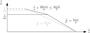
?figurename? 12: Variation of the minimal exponent

This suggests that for our theorem, it should morally be sufficient to “increase” $m^{\sharp}$ until $\bar{m}=2m^{\sharp},$ because then we would have $p_{0}^{\sharp}=2+{2\bar{m}}/(\bar{m}+m^{\sharp})={10}/{3}$. In other words, for any point $({1}/{s},1/{2p})$ fulfilling the assumptions of Theorem 1.2, we would find an $m^{\sharp}\in]m,\bar{m}/2]$ such that $({1}/{s},1/{2p})$ satisfies the requirements of Theorem 6.1 corresponding to the surface $\Gamma_{\bar{m},m^{\prime}}.$ Thus we would obtain the restriction estimate for the surface $\Gamma_{\bar{m},m^{\sharp}}$ at the point $({1}/{s},1/{2p})$. However, since this surface has “less curvature” than $\Gamma_{\bar{m},m},$ as $m^{\sharp}>m,$ the corresponding restriction inequality should hold true for $\Gamma_{\bar{m},m}=\Gamma$ as well.

To turn these heuristics into a solid proof, we just need to check that the bound for the bilinear operator that we obtained in Theorem 5.1 is increasing in $m$. Recall that for subsurfaces $S,\tilde{S}\subset S_{\bar{m},m}$ under the assumptions of the afore mentioned theorem we obtained the bound

$$\|R^{*}_{S,\tilde{S}}\|_{L^{s}(S)\times L^{s}(\tilde{S})\to L^{p}(\mathbbm{R}^{3})}$$

$$\quad\lesssim C_{\bar{m},m}:=(\rho_{1}\rho_{2})^{\frac{2}{s^{\prime}}-\frac{1}{p}}(\varkappa_{1}\rho^{2}_{1}\vee\varkappa_{2}\rho^{2}_{2})^{\frac{1}{p}-1+\varepsilon}(\varkappa_{1}\rho^{2}_{1}\wedge\varkappa_{2}\rho^{2}_{2})^{1-\frac{2}{p}-\varepsilon},$$

which we apply to $\rho_{i}=2^{-j_{i}}$ and $\varkappa_{i}=(k_{i}2^{-j_{i}})^{m_{i}-2}$ (cf. (6.6)). If we denote by $\rho_{i}^{\sharp},\varkappa_{i}^{\sharp}$ the corresponding quantities associated to the exponents $\bar{m}$ and $m^{\sharp},$ then clearly $\rho^{\sharp}_{i}=\rho_{i}$ and $\varkappa_{i}^{\sharp}\leq\varkappa_{i}.$ Since we seek to extend the range of validity of Theorem 6.1, we may assume that $2p\leq p_{0}<4$, and moreover that $2p\geq p_{0}^{\sharp}>2.$ Then we have $1/{p}-1+\varepsilon<0$ and ${1-2/{p}-\varepsilon}<0$ for sufficient small $\varepsilon>0$, and hence

$$C_{\bar{m},m}\leq(\rho^{\sharp}_{1}\rho^{\sharp}_{2})^{\frac{2}{s^{\prime}}-\frac{1}{p}}(\varkappa_{1}^{\sharp}(\rho^{\sharp}_{1})^{2}\vee\varkappa^{\sharp}_{2}(\rho^{\sharp}_{2})^{2})^{\frac{1}{p}-1+\varepsilon}(\varkappa^{\sharp}_{1}(\rho^{\sharp}_{1})^{2}\wedge\varkappa^{\sharp}_{2}(\rho^{\sharp}_{2})^{2})^{1-\frac{2}{p}-\varepsilon}=C_{\bar{m},m^{\sharp}}.$$

Proceeding with the latter estimate from here on as before in our proof of Theorem 6.1, but working now with $m^{\sharp}$ in place of $m,$ we arrive at the statement of Corollary 6.3. $\Box$

7 Appendix

7.1 A short argument to improve [FU09] to the critical line

We consider the set $A_{0}=\{x\in\mathbb{R}^{2}\,:\;1/2<|x|\leq 1\}$ and define $H={2\bar{m}}/{(2+\bar{m})}.$ Note that $H<h.$ Ferreyra and Urciuolo proved that for every $p$ for which $p>4$ and $1/{s^{\prime}}>{(H+1)}/p,$ there is a constant $C_{p,s}>0$ such that, for every function $f_{0}$ with supp $f_{0}\subset A,$ we have

$$\|R^{*}_{\mathbbm{R}^{2}}f_{0}\|_{p}\leq C_{p,s}\|f_{0}\|_{s}.$$

Re-scaling this, we obtain

$$\|R^{*}_{\mathbbm{R}^{2}}f_{j}\|_{p}\leq C_{p,s}2^{\frac{j}{h}\big{(}-\frac{1}{s^{\prime}}+\frac{h+1}{p}\big{)}}\|f_{j}\|_{s}$$ (7.1)

for every function $f_{j}$ such that supp$\,f_{j}\subset\{(x_{1},x_{2})\,:\;2^{-\frac{j+1}{m_{1}}}\leq x_{1}\leq 2^{-\frac{j}{m_{1}}},\;2^{-\frac{j+1}{m_{2}}}\leq x_{2}\leq 2^{-\frac{j}{m_{2}}}\}$ and the same range of $p,s.$

Given a function $f$ supported in the unit ball of $\mathbbm{R}^{2},$ we decompose $f=\sum_{j=0}^{\infty}f_{j},$ where the functions $f_{j}$ have supports as above. Then,

$$|\{x\,:\;|R^{*}_{\mathbbm{R}^{2}}f(x)|>\lambda\}|\leq|\{x\,:\;|\sum_{j=J}^{\infty}R^{*}_{\mathbbm{R}^{2}}f_{j}(x)|>\lambda/2\}|+|\{x\,:\;|\sum_{1}^{j=J}R^{*}_{\mathbbm{R}^{2}}f_{j}(x)|>\lambda/2\}|,$$

for some $J$ to be chosen appropriately. Using Chebyshev’s inequality, the last expression can be bounded by

$$\leq\bigg{(}\frac{2}{\lambda}\bigg{)}^{p_{1}}\|\sum_{j=J}^{\infty}R^{*}_{\mathbbm{R}^{2}}f_{j}\|_{L^{p_{1}}}^{p_{1}}+\bigg{(}\frac{2}{\lambda}\bigg{)}^{p_{2}}\|\sum_{j=1}^{J}R^{*}_{\mathbbm{R}^{2}}f_{j}\|_{L^{p_{2}}}^{p_{2}}.$$

Let us choose exponents $p_{1}>p>p_{2}$ such that $1/{s^{\prime}}={(h+1)}/p$ and ${(h+1)}/{p_{2}}>1/{s^{\prime}}>{(h+1)}/{p_{1}}>{(H+1)}/p.$ We use the triangular inequality and (7.1) and sum the resulting geometric series, obtaining the inequality

$$|\{x\,:\;|R^{*}_{\mathbbm{R}^{2}}f(x)|>\lambda\}|\lesssim\bigg{(}\frac{2}{\lambda}\bigg{)}^{p_{1}}2^{\frac{J}{h}\big{(}-\frac{p_{1}}{s^{\prime}}+{h+1}\big{)}}\|f\|_{L^{s}}^{p_{1}}+\bigg{(}\frac{2}{\lambda}\bigg{)}^{p_{2}}2^{\frac{J}{h}\big{(}-\frac{p_{2}}{s^{\prime}}+{h+1}\big{)}}\|f\|_{L^{s}}^{p_{2}}.$$

By choosing $J$ such that $2^{J}=\big{(}{\|f\|_{L^{s}}}/\lambda\big{)}^{hs^{\prime}},$ we then arrive at the weak type estimate

$$|\{x\,:\;|R^{*}_{\mathbbm{R}^{2}}f(x)|>\lambda\}|\lesssim\bigg{(}\frac{\|f\|_{L^{s}}}{\lambda}\bigg{)}^{(h+1)s^{\prime}}=\bigg{(}\frac{\|f\|_{L^{s}}}{\lambda}\bigg{)}^{p}.$$

From this, by interpolation with the trivial bound $\|R^{*}_{\mathbbm{R}^{2}}\|_{L^{1}\to L^{\infty}}\leq 1,$ we obtain the desired strong type estimate.

7.2 Faà di Bruno’s theorem and completion of the proof of Lemma 2.4

The formula of Faà di Bruno is a chain rule for higher order derivatives of the composition of two functions. This is well-known for functions in one real variable. However, we need a version for several variables.

Lemma 7.1 (Formula of Faa di Bruno).

Let $U\subset\mathbbm{R}^{n}$ and $V\subset\mathbbm{R}^{m},$ and let $g=(g^{1},\ldots,g^{m})\in C^{\infty}(U,V)$ and $f\in C^{\infty}(V,\mathbbm{R}^{l}).$ For $\alpha\in\mathbbm{N}^{n},$ we put $A_{\alpha}=\{\gamma\in\mathbbm{N}^{n}:1\leq|\gamma|\leq|\alpha|\}.$ Then $f\circ g$ is smooth, and for every $\alpha\in\mathbbm{N}^{n}$ we have

$$\partial^{\alpha}(f\circ g)=\alpha!\sum\limits_{1\leq|\beta|\leq|\alpha|}(\partial^{\beta}f)\circ g\sum\limits_{k}\prod_{j=1}^{m}\prod_{\gamma\in A_{\alpha}}\left[\frac{\partial^{\gamma}g^{j}}{\gamma!}\right]^{k_{\gamma}^{j}},$$

where the sum in $k$ is over all mappings $k:\{1,\ldots,m\}\times A_{\alpha}\to\mathbbm{N},(j,\gamma)\mapsto k_{\gamma}^{j},$ such that

$$\sum_{\gamma\in A_{\alpha}}k_{\gamma}^{j}=\beta_{j}$$ (7.1)

for all $j=1,\ldots,m$ and

$$\sum_{j=1}^{m}\sum_{\gamma\in A_{\alpha}}k_{\gamma}^{j}\gamma=\alpha.$$ (7.2)

Proof:.

The elegant short proof in [Sp05] for the one-dimensional case can easily be adapted to the higher-dimensional situation. $\Box$

We now come back to the proof of Lemma 2.4 and establish the still missing estimates for the derivatives of the function $\phi_{2}$ (given explicitly by (2.12)). Notice that these estimates can not simply be obtained by means of a scaling argument, since the first order derivatives are assumed to exhibit a different behavior than the higher order derivatives.

We shall not really make use of formula (2.12), but rather proceed as follows: denoting by $e_{1},\dots,e_{d+1}$ the canonical basis of $\mathbbm{R}^{d+1},$ after applying a suitable orthogonal transformation to $\mathbbm{R}^{d+1}$ we may and shall assume that $n_{1}=(0,\dots,0,1)=e_{d+1},$ and that $E_{1}=e_{1},\dots,E_{d-1}=e_{d-1}$ and $e_{d}=h_{1}$ (recall here from the first part of the proof of Lemma 2.4 that $E_{1},\dots,E_{d-1}$ is an orthonormal basis of $K=H_{1}\cap H_{2}$). Then we may regard $U_{1}$ as a subset of $\mathbbm{R}^{d},$ and we consider the function

$$H(\eta,\tau)=\tau-\phi_{1}(\eta),\qquad\eta\in U_{1},\tau\in\mathbbm{R},$$

whose set of zeros agrees exactly with $S.$ Observe first that the derivatives of $H$ satisfy almost the same kind of estimates as $\phi_{1}:$

$$\|H^{\prime}\|_{\infty}\leq \sqrt{A^{2}+1},\quad\|H^{(l)}\|_{\infty}\leq A_{l}Br^{l}\quad\mbox{for every }l\geq 2.$$ (7.3)

Let $\psi(\xi)=\xi+\phi_{2}(\xi)n_{2},\ \xi\in U_{2},$ be the parametrization of $S$ induced by $\phi_{2}.$ Moreover, we introduce coordinates on $U_{2}$ by writing $\xi=\xi_{1}E_{1}+\cdots+\xi_{d-1}E_{d-1}+\xi_{d}h_{2}.$ Then obviously

$$H(\psi(\xi))=0\quad\mbox{for all}\quad\xi\in U_{2}.$$ (7.4)

Furthermore,

$$\frac{\partial\psi}{\partial\xi_{j}}=E_{j}+\frac{\partial\phi_{2}}{\partial\xi_{j}}n_{2},\quad j=1,\ldots,d-1,\quad\frac{\partial\psi}{\partial\xi_{d}}=h_{2}+\frac{\partial\phi_{2}}{\partial\xi_{d}}n_{2},$$ (7.5)

and

$$\partial_{\xi}^{\alpha}\psi=\partial_{\xi}^{\alpha}\phi_{2}\,n_{2}\quad\mbox{for all}\quad\alpha\in\mathbbm{N}^{d},|\alpha|\geq 2.$$ (7.6)

From (7.4) and (7.5) we obtain that for $j=1,\dots,d,$

$$\frac{\partial\phi_{2}}{\partial\xi_{j}}(\xi)=-\frac{\langle(\nabla H)(\psi(\xi)),\tilde{e}_{j}\rangle}{\langle(\nabla H)(\psi(\xi)),n_{2}\rangle},$$ (7.7)

if we put $\tilde{e}_{j}=E_{j}=e_{j},$ if $j=1,\dots,d-1$ and $\tilde{e}_{d}=h_{2}.$ Notice also that our transversality condition $|\langle n_{2},N(v)\rangle|\geq a>0$ for all $v\in S$ implies that $|\langle(\nabla H)(\psi(\xi)),n_{2}\rangle|\geq a.$ Thus (7.7) implies that

$$\big{|}\frac{\partial\phi_{2}}{\partial\xi_{j}}(\xi)\big{|}\leq\frac{A+1}{a}.$$ (7.8)

It remains to show that

$$\|\partial^{\alpha}\phi_{2}\|_{\infty}=\|\partial^{\alpha}\psi\|_{\infty}\leq \tilde{A}_{l}Br^{|\alpha|}$$ (7.9)

for every $|\alpha|\geq 2,$ where we have used the abbreviation $\partial=\partial_{\xi}.$ By induction, we may assume that for every $\gamma\in\mathbbm{N}^{d}$ with $2\leq|\gamma|<|\alpha|$ inequality (7.9) holds true. Applying the partial derivative of order $\alpha$ to (7.4) yields

$$\partial^{\alpha}(H\circ\psi)=0.$$

We apply the formula of Faà di Bruno (Lemma 7.1). First, we discuss the summands in Faà di Bruno formula with $|\beta|=1$, say $\beta=e_{j_{0}}$ for some $j_{0}=1,\ldots,m$. How many $k$’s are there for which $\sum_{\gamma\in A_{\alpha}}k_{\gamma}^{j}=\beta_{j}=\delta_{jj_{0}}$ and $\sum_{j=1}^{m}\sum_{\gamma\in A_{\alpha}}k_{\gamma}^{j}\gamma=\alpha$? By the first condition, there exists a $\gamma_{0}$ such that $k^{j_{0}}_{\gamma_{0}}=1$ and $k^{j}_{\gamma}=0$ for $j\neq j_{0}$ or $\gamma\neq\gamma_{0}$. But then the second condition implies that $\gamma_{0}=\alpha$. Thus we obtain

$$\sum\limits_{|\beta|=1}(\partial^{\beta}H)\circ\psi\sum\limits_{k}\prod_{j=1}^{m}\prod_{\gamma\in A_{\alpha}}\left[\frac{\partial^{\gamma}\psi^{j}}{\gamma!}\right]^{k_{\gamma}^{j}}=\sum_{j_{0}=1}^{m}(\partial_{j_{0}}H)\circ\psi\left[\frac{\partial^{\alpha}\psi^{j_{0}}}{\alpha!}\right]^{k_{\alpha}^{j_{0}}}$$

$$=\frac{1}{\alpha!}\langle(\nabla H)\circ\psi,\partial^{\alpha}\psi\rangle=\frac{\partial^{\alpha}\phi_{2}}{\alpha!}\langle(\nabla H)\circ\psi,n_{2}\rangle,$$

where we have used (7.6) once more. This implies that

$$|\partial^{\alpha}\phi_{2}|\leq \frac{\alpha!}{a}\left|\sum\limits_{|\beta|=2}^{|\alpha|}(\partial^{\beta}H)\circ\psi\sum\limits_{k}\prod_{j=1}^{m}\prod_{\gamma\in A_{\alpha}}\left[\frac{\partial^{\gamma}\psi^{j}}{\gamma!}\right]^{k_{\gamma}^{j}}\right|,$$

where the sum in $k$ is over all mappings $k:\{1,\ldots,m\}\times A_{\alpha}\to\mathbbm{N},(j,\gamma)\mapsto k_{\gamma}^{j}$ such that $\sum_{\gamma\in A_{\alpha}}k_{\gamma}^{j}=\beta_{j}$ for all $j=1,\ldots,m$ and $\sum_{j=1}^{m}\sum_{\gamma\in A_{\alpha}}k_{\gamma}^{j}\gamma=\alpha$. Observe that for all $k$ appearing in the above sum, we have $k^{j}_{\alpha}=0$ for all $j=1,\ldots,m$:

For, otherwise there would be some $j_{0}$ such that $k_{\alpha}^{j_{0}}=1$ and $k_{\gamma}^{j}=0$ if $\gamma\neq\alpha$ or $j\neq j_{0}$, a contradiction to $2\leq|\beta|=\sum_{j,\gamma}k_{\gamma}^{j}$.
Thus, if $k_{\gamma}^{j}\neq 0$ for an exponent in the above sum, then we have $|\gamma|<|\alpha|,$ and therefore our induction hypothesis applies the following:

If $|\gamma|\geq 2$, then we may estimate $|\partial^{\gamma}\psi^{j}|\leq A_{|\gamma|}Br^{|\gamma|}.$ And, if $|\gamma|=1$, then in view of (7.5) and (7.8), we may estimate $|\partial^{\gamma}\psi^{j}|\leq 1+(A+1)/a\lesssim 1.$ Making also use of (7.3), we then arrive at the estimation

$$|\partial^{\alpha}\phi_{2}|\lesssim \sum\limits_{|\beta|=2}^{|\alpha|}Br^{|\beta|}\sum\limits_{k}\prod_{j=1}^{m}\prod_{|\gamma|=2}^{|\alpha|}\left[Br^{|\gamma|}\right]^{k_{\gamma}^{j}}$$

$$\leq \sum\limits_{|\beta|=2}^{|\alpha|}\sum\limits_{k}B^{1+\sum_{j}\sum_{|\gamma|=2}^{|\alpha|}k_{\gamma}^{j}}\ r^{|\beta|+\sum_{j}\sum_{|\gamma|=2}^{|\alpha|}k_{\gamma}^{j}|\gamma|}.$$

Notice that we have

$$|\beta|=\sum_{j}\beta_{j}= \sum_{j}\sum_{|\gamma|=1}^{|\alpha|}k_{\gamma}^{j}=\sum_{j}\sum_{|\gamma|=2}^{|\alpha|}k_{\gamma}^{j}+\sum_{j}\sum_{|\gamma|=1}k_{\gamma}^{j}|\gamma|,$$

and thus

$$B^{1+\sum_{j}\sum_{|\gamma|=2}^{|\alpha|}k_{\gamma}^{j}}r^{|\beta|+\sum_{j}\sum_{|\gamma|=2}^{|\alpha|}k_{\gamma}^{j}|\gamma|}=Br^{\sum_{j}\sum_{|\gamma|=1}^{|\alpha|}k_{\gamma}^{j}|\gamma|}(Br)^{\sum_{j}\sum_{|\gamma|=2}^{|\alpha|}k_{\gamma}^{j}}\leq Br^{|\alpha|},$$

where we have made use of our assumption $Br\leq 1$. This proves also (7.9).

References

- [Ba85] B. Barcelo Taberner, On the restriction of the Fourier transform to a conical surface, Transactions of the American Mathematical Society, 292 No1 (1985).
- [Ba86] B. Barcelo, The restriction of the Fourier transform to some curves and surfaces, Studia Mathematica 84 No1 (1986), 39–69.
- [BCT06] J. Bennet, A. Carbery, T. Tao, On the multilinear restriction and Kakeya conjectures. Acta Math. 196 (2006), no. 2, 261–302.
- [Bou85] Bourgain, J., Estimations de certaines fonctions maximales. C. R. Acad. Sci. Paris Sér. I Math., 301 (1985) no. 10, 499–502.
- [Bo91] J. Bourgain, Besicovitch-type maximal operators and applications to Fourier analysis, Geometric and Functional Analysis 22 (1991), 147-187.
- [Bo95a] J. Bourgain, Some new estimates on oscillatory integrals. Essays in Fourier Analysis in honor of E. M. Stein. Princeton Math. Ser. 42, Princeton University Press, Princeton, NJ 1995, 83–112.
- [Bo95b] J. Bourgain, Estimates for cone multipliers, Operator Theory: Advances and Applications 77 (1995), 1-16.
- [BoG11] J. Bourgain, L. Guth, Bounds on oscillatory integral operators based on multilinear estimates, Geometric and Functional Analysis, Vol.21 (2011) 1239-1295.
- [Bu15] S. Buschenhenke, A sharp - Fourier restriction theorem for a conical surface of finite type, Mathematische Zeitschrift, Vol. 280, Issue 1 (2015), 367-399.
- [F70] C. Fefferman, Inequalities for strongly singular convolution operators. Acta Math., (1970), 9–36.
- [F71] C. Fefferman, The multiplier problem for the ball, Annals of Mathematics 94 (1971) 330-336.
- [FU09] E. Ferreyra, M. Urciuolo, Fourier restriction estimates to mixed homogeneous surfaces, Journal of inequalities in pure and applied mathematics, Vol. 10 (2009) Issue 2, Article 35, pp. 11.
- [Gra08] L. Grafakos, Classical Fourier Analysis, Graduate Texts in Mathematics, Springer, 2008.
- [Gr81] A. Greenleaf, Principal Curvature and Harmonic Analysis, Indiana University Mathematics Journal, Vol. 30, No. 4 (1981).
- [IKM10] I. A. Ikromov, M. Kempe, D. Müller, Estimates for maximal functions associated with hypersurfaces in and related problems in harmonic analysis, Acta Mathematica 204 (2010), 151-271.
- [IM11] I. A. Ikromov, D. Müller, Uniform estimates for the Fourier transform of surface carried measures in and an application to Fourier restriction. J. Fourier Anal. Appl., 17 (2011), no. 6, 1292–1332.
- [IM15] Ikromov, Müller, Fourier Restriction for Hypersurfaces in Three Dimensions and Newton Polyhedra, Part I and II; http://arxiv.org/abs/1208.6090 and http://arxiv.org/abs/1410.3298; to appear Annals of Mathematics Studies.
- [L03] S. Lee, Endpoint estimates for the circular maximal function, Proc. Amer. Math. Soc. 131 (5) (2003) 1433–1442.
- [L05] S. Lee, Bilinear restriction estimates for surfaces with curvatures of different signs, Transactions of the American Mathematical Society, Vol. 358, No. 8, 3511-2533, 2005.
- [LV10] S. Lee, A. Vargas, Restriction estimates for some surfaces with vanishing curvatures, Journal of Functional Analysis 258 (2010), 2884-2909.
- [MVV96] Moyua, A., Vargas, A. and L. Vega, L., Schrödinger maximal function and restriction properties of the Fourier transform. Internat. Math. Res. Notices 16 (1996), 793–815.
- [MVV99] Moyua, A., Vargas, A. and L. Vega, L., Restriction theorems and maximal operators related to oscillatory integrals in Duke Math. J., 96 (3), (1999), 547-574.
- [S87] C. D. Sogge, A sharp restriction theorem for degenerate curves in , American Journal of Mathematics, Vol. 109, No. 2 (1987), pp. 223-228.
- [Sp05] K. Spindler, A short proof of the formula of Fa\adi Bruno, Elemente der Mathematik, Swiss Mathematical Society (2005), 33-35.
- [St86] E. Stein, Oscillatory Integrals in Fourier Analysis. Beijing Lectures in Harmonic Analysis. Princeton Univ. Press 1986.
- [Sto15] B. Stovall, Linear and bilinear restriction to certain rotationally symmetric hypersurfaces. Preprint 2015.
- [Str77] Strichartz, R. S.,Restrictions of Fourier transforms to quadratic surfaces and decay of solutions of wave equations. Duke Math. J. 44 (1977), no. 3, 705–714.
- [T01a] T. Tao Endpoint bilinear restriction theorems for the cone, and some sharp null-form estimates, Math. Z. 238 (2001), 215-268.solutions of wave equations. Duke Math. J., 44 (1977), 705–714.
- [T01b] T. Tao, From Rotating Needles to stability of waves: emerging connections between combinatorics, analysis, and PDE, Notices of the American Mathematical Society, 48 (2001).
- [T03a] T. Tao, A Sharp bilinear restriction estimate for paraboloids, Geometric and Functional Analysis 13, 1359-1384, 2003.
- [T03b] T. Tao, Recent progress on the Restriction conjecture, arXiv:math/0311181v1 [math.CA] 12 Nov 2003.
- [To75] P. A. Tomas, A restriction theorem for the Fourier transform. Bull. Amer. Math. Soc. 81 (1975), 477–478.
- [TVI00] T. Tao, A. Vargas, A bilinear approach to cone multipliers I. Restriction estimates, Geometric and Functional Analysis 10, 185-215, 2000.
- [TVII00] T. Tao, A. Vargas, A bilinear approach to cone multipliers II. Applications, Geometric and Functional Analysis 10, 216-258, 2000.
- [TVV98] Tao, T., Vargas, A. and Vega, L., A bilinear approach to the restriction and Kakeya conjectures. J. Amer. Math. Soc. 11 (1998) no. 4 , 967–1000.
- [V05] A. Vargas, Restriction theorems for a surface with negative curvature, Mathematische Zeitschrift 249, 97-111 (2005).
- [W95] T. Wolff, An improved bound for Kakeya type maximal functions, Revista Mat. Iberoamericana 11 (1995), 651-674.
- [W01] WT. Wolff, A Sharp Bilinear Cone Restriction Estimate, The Annals of Mathematics, Second Series, Vol. 153, No. 3, 661-698, 2001.
- [Z74] A. Zygmund, On Fourier coefficients and transforms of functions of two variables, Studia Mathematica 50 (1974), 189-201.