Two step robust fringe analysis method
with random shift
Abstract
We propose a two steps fringe analysis method assuming random phase step and changes in the illumination conditions. Our method constructs on a Gabor Filter–Bank (GFB) that independently estimates the phase from the fringe patterns and filters noise. As result of the GFB we obtain the two phase maps except by a random sign map. We show that such a random sign map is common to the independently computed phases and can be estimated from the residual between the phases. We estimate the final phase with a robust unwrapping procedure that interpolates unreliable phase regions. We present numerical experiments with synthetic and real date that demonstrate our method performance.
1 Method
In recent years there has been an interest for developing two–steps algorithms with random step; see for example the methods in [2, 3, 4, 5] and references therein. Those techniques have significantly reduced the acquisition time and have simplified the experimental setups. In this work we propose a robust algorithm that can overcome the limitation of random two-steps algorithms for dealing with variable illumination condition and noise. The proposed method is able to estimate the phase from two noise fringe pattern (FP) with a random phase step between them including temporal variations in illumination conditions and noise. We proceed as follows: first we motivate our algorithm and then we present the details.
In this work we assume the following FPs models
| (1) | |||||
| (2) |
where denotes the pixel position in a regular lattice . The unknowns are: the background illumination, and ; the local fringe contrast, and ; the independent noise, and ; the phase map we are interested in computing, ; and the random shift between the FPs, . In this work, we consider the standard assumptions used in single FP algorithms: , (for ), and are smooth.
Essentially the proposed method consists of three stage. Firstly, estimation of the wrapped phase with a sign ambiguity, this os obtain by using the operator. Second, estimation of the correct sign map based on the operator that computes the wrapped residual phase between a pair of phase map. Finally, we present a robust unwrap process, denoted by the operator , that interpolates unreliable estimated phase pixels. Following we define the method and the operators. After that, we provide the details.
Assume we have a method, represented for the operator , such that:
| (3) | |||||
| (4) |
where is a random sign field and is the phase wrapping operator, see [6]. Next, we use the operator that computed the residual wrapped phase between two given phases and . This operator is denoted by
| (5) |
where is the unwrapping operator, see [6]. Since , we obtain . Thus, we can estimate the sign with
| (6) |
Let be the wrapped computed phase; then, we can finally estimate the phase with
| (7) |
Essentially, this is the proposed method. Now we specify each one of the used operators: phase analysis (), residual phase () and unwrapping ().
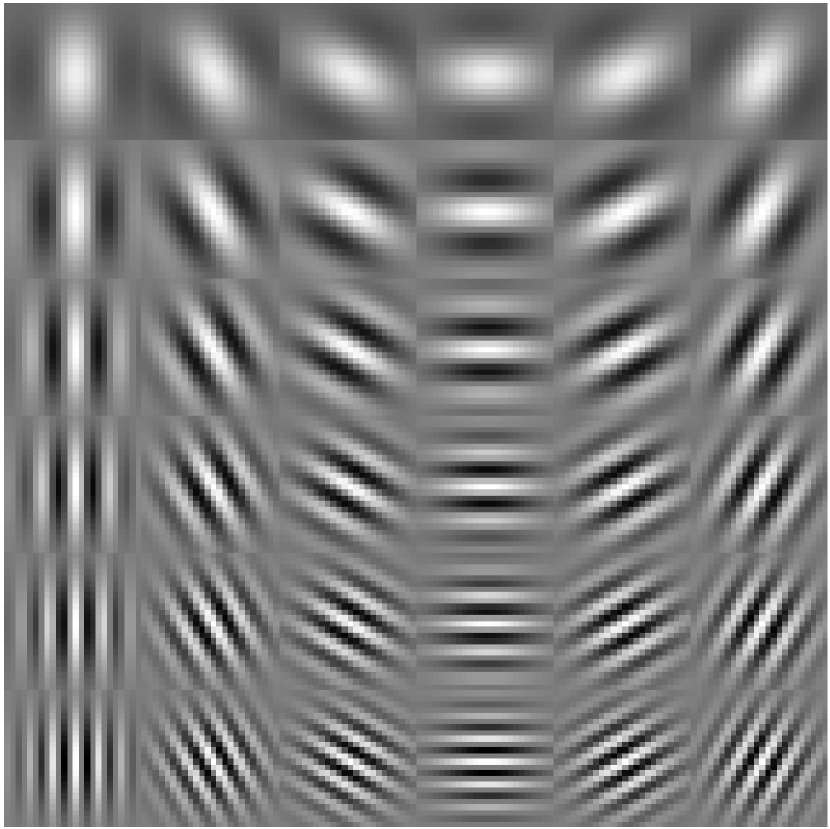
Robust Phase Analysis, . In order to compute the local phase from a noisy FP with variation in the background illumination and contrast, and closed fringes, one can use a general closed fringe method which simultaneously estimates the phase and the sign. However, those methods are computationally expensive. Therefore, as we have stated, our proposal takes advantage of the second shifted–FP for estimating the sign. Then we propose to use a Gabor’s Filter-Bank (GFB); i.e., a set of narrowband filters that only cover a half of the Discrete Fourier Domain and rejects: low-pass region related with the background illumination (DC) spectra and very-high frequencies assumed noise. Gabor Filters (GF) are bandpass filters which are obtained by modulating a sinusoid with a Gaussian [7]. The complex form of the convolution kernel is
| (8) |
where
| (9) |
| (10) |
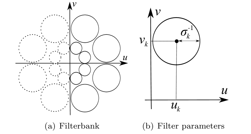
with , the width of the Gaussian filter (bandwidth of the bandpass filter) and the central complex frequency (center of the bandpass filter). The GF (8) can be understood by transforming it to the Fourier space. The transform of the term corresponds to a Dirac delta centred at , , and the transform of the Gaussian is another Gaussian . Then, by the convolution theorem of the Fourier transform, the Gabor filter in the frequency domain is given by ; see Figure 2.
Hence, the result of applying the th GF to the th fringe pattern is given by:
| (11) |
where denotes the convolution. is complex and expressed in rectangular coordinates (real and imaginary parts), the respective polar coordinates (magnitude and phase) are computed with
| (12) | |||||
| (13) |
for . Since the FP has locally a dominant frequency, in order to estimate the phase and magnitude at each pixel, we detect the filter with maximum response (the best tuned filter to the local frequency of the FP):
| (14) |
Thus, the magnitude and phase corresponding to the pixel, in the FP, is
| (15) | |||||
| (16) |
Since there exists a winner filter at each pixel, , we obtain a phase at each pixel even if the pixel in question belongs to a low frequency region (pixels in region with almost constant phase). In such a case, the GFB will be activated by white noise . To reduce such a noise detection, we use the computed magnitude as a confidence measure of the computed phase. We compute the mask of reliable phase with
| (17) |
where the threshold is a parameter of the method. In our experiments we use a single set of parameters for the GFB: such parameters are illustrated in Fig. 3.
Phase differences, . The next step is to implement (5) for computing the phase differences between the two estimated phases and . According to [6], the wrapped residual between two phases can be computed without explicit knowledge of with
| (18) |
using the identities:
| (19) |
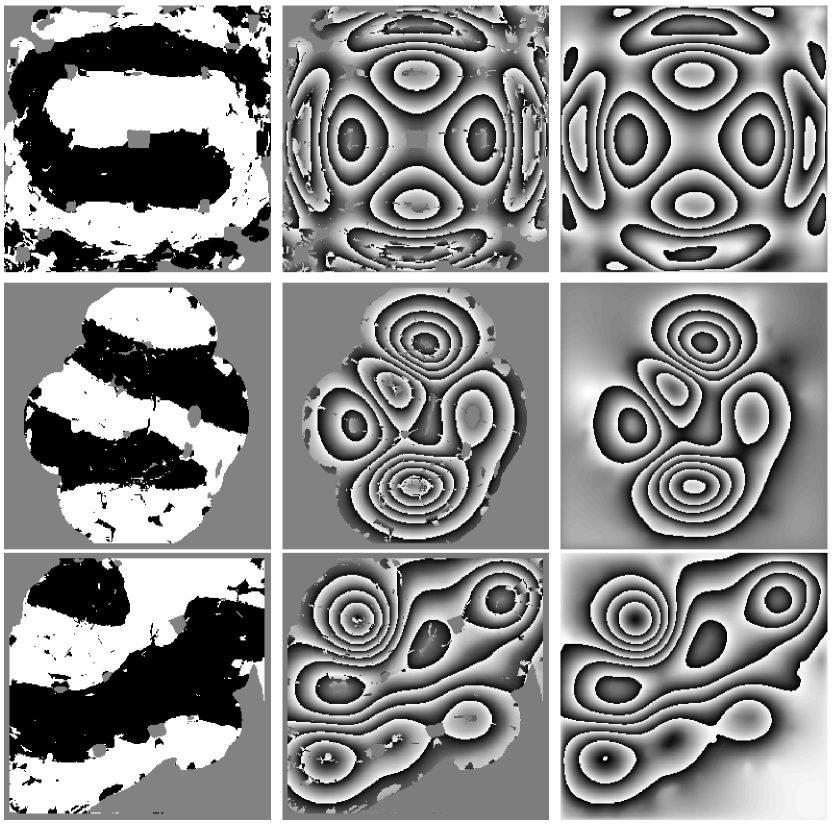
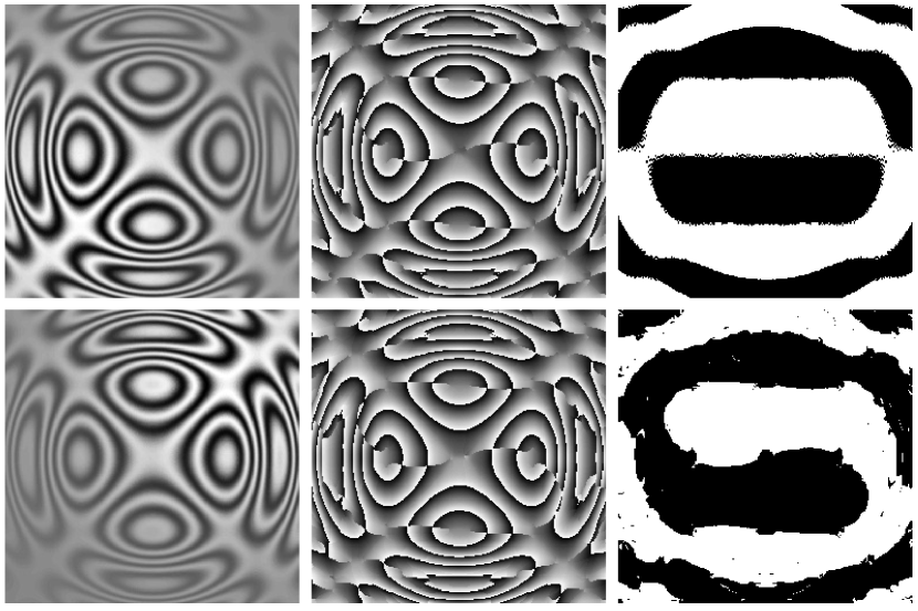
Robust phase unwrapping, . The last step is to unwrap the phase taking into account that the computed sign–map can be corrupted by errors: compare sign–maps in third column of Fig. 1 and experimental results in Fig. 5. We note that the sign is prone to be incorrectly computed at regions where the magnitude of the phase gradients are small (regions with almost constant phase). Such regions can be detected with the mask defined in (17).
In this work we use a variant of the unwrapping algorithm recently reported in [6]. The algorithm iteratively update the current estimate of the unwrapped phase with an unwrapped update phase :
| (20) |
where the updating field is computed by
| (21) |
where and are positive parameters and we define
| (22) |
and the set of first neighbour pixels to the pixel as
| (23) |
We modified the cost function (21) by introducing the binary weights and [see (17)] that define the region with reliable data. Hence, the phase at regions with invalid data are smoothly interpolated by effect of the regularization.
2 Experiments and Conclusions
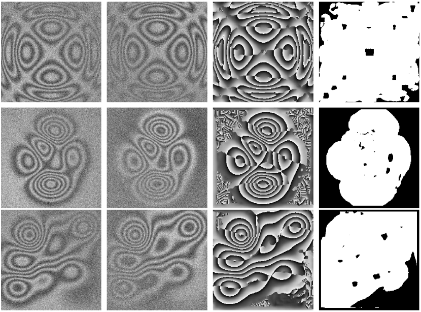
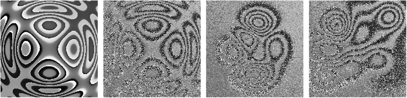
Figures 4 and 5 demonstrate the proposed method’s performance. The test FP are shown in Fig. 4: we use the same contrast modulation, and , as in the FPs of Fig. 1. The GFB robustly and independently estimate the phase, except by the random sign, of each FP with different background illumination (), contrast (), and corrupted with independent noise (). An advantage of the GFB is that one can obtain the quality map that defines regions where the estimated phase is reliable. Then, the proposed unwrapping procedure can effectively interpolate the missed phase regions.
Gram–Schmidt based orthonormalization (GSBO) has shown to be a computationally efficient method for computing a couple of quadrature images [3]. That interesting proposal has motivated works for overcoming its drawbacks: the performance of such a method is limited when there are variations in the background, contrast and noise; see Fig. 6.
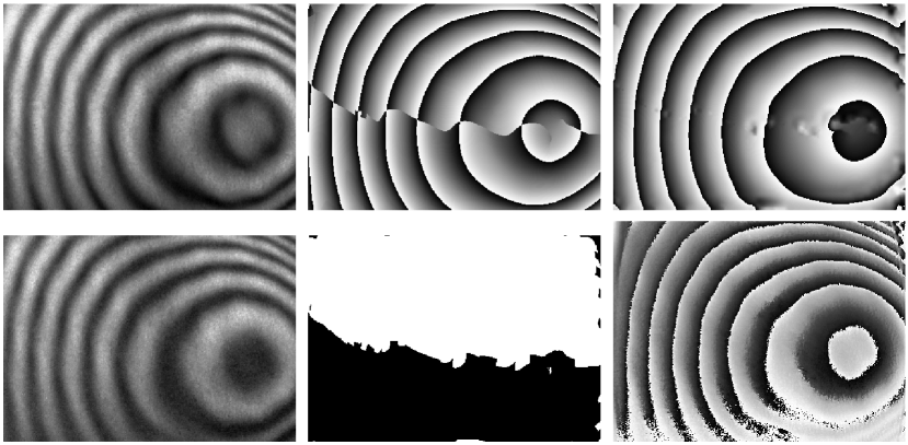
Fig. 7 shows the coupled phase with the proposed method using as test FP real interferograms. The used parameters of the filterbank, expressed in polar coordinates, are and ; with and . We can observe that our method correctly recover the phase. In contrast, we can note that GSBO fails to compute a phase even when the FP have a phase shift equals . The reason of the GSBO’s poor performance is the large changes in the illumination conditions. The GSBO approach can be improved by using a windows-wise technique [4]. Although this technique can reduce the effect of variation in illumination components, the main drawback is that it requires a window size that includes several fringe fringes, with the additional limitation of processing low frequency FP. In the best of our knowledge, the best procedure for reducing all the mentioned differences is by preprocessing the FPs with banks of quadrature filters (as GFB). In our work, we use the GBF as part of our process. The reader can find limitation of other two-step demodulation algorithms in [3, 4, 5]. In [5] it is described a sophisticated preprocess for normalising the fringes in order to apply GSBO. The result of such a prefiltering is similar in our approach to apply the GFB. However, differently to [5] that requires the additional step of GSBO for estimating the phase with the correct sign, in our case, the correction sign map is obtained directly from the GFB result; i.e., we do need the extra orthonormalization step.
References
- [1]
- [2] J. Deng, H. Wang, F. Zhang, D. Zhang, L. Zhong, and X. Lu, Opt. Lett., 37, 4669 (2012).
- [3] J. Vargas, J. A. Quiroga, C. O. S. Sorzano, J. C. Estrada, and J. M. Carazo, Opt. Lett., 37, 443 (2012).
- [4] J. Ma, Z. Wang, and T. Pan, Optics and Lasers in Engineering 55, 205 (2014).
- [5] M. Trusiak and K. Patorski, Opt. Exp., 23, 4672 (2015)
- [6] M. Rivera, F. J. Hernandez-Lopez, and A. Gonzalez, Optics and Lasers in Engineering 64, 51 (2015).
- [7] J. Daugman, Acoustics, Speech and Signal Processing, IEEE Transactions on 36, 1169 (1988).