Bursting noise in gene expression dynamics:
Linking microscopic and mesoscopic models

Abstract

The dynamics of short-lived mRNA results in bursts of protein production in gene regulatory networks. We investigate the propagation of bursting noise between different levels of mathematical modelling, and demonstrate that conventional approaches based on diffusion approximations can fail to capture bursting noise. An alternative coarse-grained model, the so-called piecewise deterministic Markov process (PDMP), is seen to outperform the diffusion approximation in biologically relevant parameter regimes. We provide a systematic embedding of the PDMP model into the landscape of existing approaches, and we present analytical methods to calculate its stationary distribution and switching frequencies.

Transcription and translation in the process of gene expression occur at the molecular level and in environments of relatively small copy numbers. The discreteness of the molecular dynamics and the inherent randomness with which reactions occur are known as ‘intrinsic noise’. It is now widely accepted that intrinsic noise plays an important role in gene regulatory networks^{1; 2; 3}. It promotes epigenetic diversity and enhances the adaptability of a single phenotype in changing environments ^{4; 5}. To investigate the effects of intrinsic noise, mathematical models at different levels have been constructed, ranging from microscopic models ^{6; 7; 3; 8; 9; 10} describing the finer origins of intrinsic noise to mesoscopic models^{11; 12; 13; 14; 15}. While the former capture the biological processes in more detail, the latter are computationally scalable and constructed to model more complex networks. These models all capture some signatures of intrinsic noise, but the detailed implementation of stochasticity varies from model to model. It is then important to consider how noise propagates between different levels of mathematical modelling. At present coarse-grained models are often proposed ad hoc and not derived from the more detailed lower-scale models. Is this always mathematically appropriate? What statistics of noise should modellers use at the different levels of coarse graining? What are the consequences of the choice of noise statistics, and what are the pitfalls in deriving models on the meso-level from finer models on smaller scales? These are some of the questions we aim to address in this work.

The above difficulties in transitioning between different levels of modelling can nicely be illustrated in the context of biological switches. These are systems with different metastable states and the possibility to ‘switch’ between those states. Biological organisms with such behaviour include the Lac switch ⁶ in Escherichia coli and the Enterobacteria phage $\lambda$ switch ⁷. Computational and mathematical models of these range from very detailed descriptions ^{6; 7} over individual-molecule approaches ^{9; 8; 16; 10} to mesoscopic models ^{11; 12; 14; 15}.

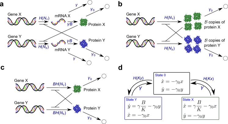
Figure 1: Schematic diagrams illustrating the model dynamics. (a) Full model (FM) describing both the mRNA and the protein populations; (b) Protein-only model with geometrically distributed (GB) or constant (CB) bursts. The quantity $\mathcal{B}$ is a geometrically distributed random number with mean $B$ in the GB model, and $\mathcal{B}=B$ is a constant in the CB model; (c) Protein-only model without bursts (NB); (d) The piecewise deterministic Markov process (PDMP).

The difficulties in connecting these different levels of modelling biological switches are amplified by the recent recognition that the mRNA populations are essential to describing the statistics of regulatory processes ^{17; 16}. Biologically, mRNA molecules are a relatively short-lived source compared to the proteins into which they ultimately translate. Protein production from a given mRNA molecule proceeds while it exists, but ceases after the mRNA decays. This leads to a production of protein in bursts—that is, the production is active for a relatively short and random period of mRNA lifetime, and during that time a random number of proteins is generated. This phenomenon is termed translational bursting ¹ and it can be observed in single-molecule experiments ¹⁸. While some mesoscopic models account for such bursting ^{14; 15}, the theoretical investigation of these processes is often limited to their stationary distribution and frequently does not include dynamic features such as switching times.

The aim of our work is to investigate the effects bursting noise in gene regulatory networks ^{19; 9; 16; 20; 10; 11; 13; 21}, and to construct connections between individual-based models and mesoscopic approaches. Specifically, we start from microscopic and individual-molecule-based models of a toggle switch and set out to construct coarse grained, mathematically tractable models without systematically biasing the outcomes.

I Results

Different scales of individual-based models of a toggle switch network. We compare four individual-based models and investigate the effect of bursting noise in a toggle switch network. The first model we consider describes both the mRNA and the protein population dynamics¹⁶. Fig. 1a illustrates the Markovian model of the regulatory network. Genes X and Y are transcribed into mRNA X and mRNA Y, respectively, which in turn are translated to produce proteins X and Y. The transcription of each of the two genes is suppressed by proteins of the respective other type via a Hill function^{2; 3} $H(N)=K\left[r_{0}+r/[1+(N/K)^{n}]\right]$, where $N$ stands for the number of suppressing proteins. The model parameter $K$ represents a typical population scale of the proteins, and the parameters $r$ and $r_{0}$ set the minimal ($r_{0}K$) and maximal transcription rates ($(r_{0}+r)K$). The parameter $n>0$ is the so-called Hill coefficient which models the cooperative binding of the repressors ³. More details of the reaction scheme can be found in the Supplementary Information. Proteins of either type, and the mRNA molecules degrade with constant rates $\gamma_{0}$ and $\gamma$ respectively. Biologically, mRNA molecules degrade much faster than the proteins do ($\gamma\gg\gamma_{0}$) ^{2; 14; 18}. The translation rate of the mRNA is parametrised by $\gamma B$ where the parameter $B$ is the relative frequency of protein production to mRNA degradation. In this parametrisation, the number of proteins one single mRNA molecule produces during its lifetime is a geometrically distribution random variable with mean $B$ (see Supplementary Information). Biologically the parameter $B$ varies depending on the type of product protein ²⁴. We assume $B\gtrsim 10$ in this work ^{2; 8} to investigate the effect of translational bursting. Together with the relatively short lifetime of mRNA molecules, this constitutes the origin of ‘translational bursting’ in the model ^{14; 25}: a relatively large number of protein molecules is synthesized in a relatively short period of time.

Parameter	Description	Value	Unit	Reference
$B$	Average number of protein each mRNA produces	30	molecule	2
$\gamma$	mRNA degradation rate	30	1/(cell cycle)	2
$\gamma_{0}$	Protein degradation rate	1.0	1/(cell cycle)	2; 9; 22
$r$	Maximum suppressed transcription rate	$6/100$	1/(cell cycle)	13; 23
$r_{0}$	Basal transcription rate	$1/150$	1/(cell cycle)	13; 23
$K$	A typical population scale of the proteins	200	molecule	13; 23
$n$	Hill coefficient	3.0	Dimensionless	9; 19; 13; 23

Table 1: Parameter set.

For simplicity, the process in Fig. 1a is assumed to be symmetric with respect to X and Y, but the analysis is easily generalised to asymmetric circuits. In Table 1 we list a set of estimated values of the parameters for the model organism E. coli, along with relevant references.

In the context of this work the model just described constitutes the most detailed model we will investigate and compare against. It serves as a starting point for the derivation of more coarse grained models, and for these purposes we will refer to it as the ‘full model’ (FM) in the following.

The FM describes both the mRNA and the protein populations, hence it constitutes a relatively high-dimensional system which complicates the mathematical analysis. Notably, the only role of mRNA in the FM is to generate proteins, and so mRNA can be left out, so long as the correct statistics of protein production is retained. The timescale separation between the mRNA and protein lifetimes leads to the following reduced model describing only the protein dynamics. In the limit of infinitely-fast mRNA degradation ($\gamma\gg\gamma_{0}$), proteins are generated instantaneously in bursts of geometrically distributed sizes with a mean $B$, and in between bursting events protein populations decay with rate $\gamma_{0}$. We will refer to the reduced model as the GB model (geometrically distributed bursts), see Fig. 1b ^{24; 17}. In the GB model, the transcription rates are regulated via the Hill function exactly as before in the FM.

A further reduction of the GB model involves replacing the geometrically distributed burst sizes by a constant size $B$. We will call this the CB model (constant bursts) ⁸. While the reduction of the full model to the model with geometrically distributed bursts is well controlled and exact in the limit $\gamma\gg\gamma_{0}$, the effects of introducing constant burst sizes are unclear at this stage, and require a detailed analysis (see below).

An even more reduced model is a model with no bursts^{10; 9; 8}, we will refer to this as the NB model. The reaction scheme is illustrated in Fig. 1c. In this model, only one single protein is synthesized when a transcription event occurs. We assume a $B$-fold increased transcription rate so that the average number of proteins synthesized per unit time is consistent with the FM, GB, and CB models.

Only the GB model approximates the stationary distribution of the FM. Numerical simulations of each of the models are carried out using standard methods ^{26; 27}. In the following we present statistical properties of the models, leaving typical sample paths to the Supplementary Information. Fig. 2 displays the numerically computed stationary distributions for the FM, GB, CB and NB models. They illustrate that the profiles of protein expressions in different model settings are quite distinct. This is due to the different representation of the underlying intrinsic noise.

While the stationary distributions of the FM and the GB model are in good agreement with each other, substantial discrepancies from the full model are found in the CB and NB models. In the CB model the stationary distribution of protein numbers is very localised compared to the FM and the GB model. In the NB model the probability distribution is even more sharply concentrated. This is because the NB model misses out two pertinent sources of noise. Bursting production in the CB model amplifies the stochasticity of transcription events and leads to a broadening of the protein distribution. Adding randomly distributed burst sizes (GB model) introduces further stochasticity, and diversifies of protein numbers even further.

Based on these results, we conclude that the bursting noise introduced by the mRNA populations significantly broadens the stationary distribution. In addition, the GB model approximates the FM model significantly better than the CB and NB models do. We can effectively discard the CB and NB models as faithful representation of the FM, and our subsequent discussion hence focuses mostly on the GB model.

The GB model approximates the mean first switching time of the FM. The toggle switch has two dynamic attractors, one in which protein X is highly expressed and where protein Y has a low concentration, and the other with inverted roles by symmetry. Starting from one attractor the switch can be driven to the other attractor by fluctuations. The timescale of such a transition quantifies the dynamical stability: the longer the timescale, the more stable the system is at the initial position. As we will study next, the way in which the bursting production of protein is implemented significantly affects the timescale of these switching processes.

Starting from initial condition $N_{\rm X}(0)=n_{x,0}$ and $N_{\rm Y}(0)=n_{y,0}$, we define the first switching time as the time it takes a sample path to reach the symmetric boundary $N_{\rm X}=N_{\rm Y}$. Mathematically, the first switching time is a random variable. The mean first switching time (MFST) is then the average value of the random first switching time. The MFST depends on the initial condition $\left(n_{x,0},n_{y,0}\right)$.

Sweeping across the space of possible initial configuration, the MFST of the FM and of the GB model are measured in simulations and presented in Fig. 3. We show the MFST of the CB in the Supplementary Information. As with the stationary distributions, the data in Fig. 3 indicates that the GB model approximates the switching times of the full model to a good accuracy. We remark that the MFST of the CB model is almost as twice as long as that of the GB and FM models, and the switching time in the NB model is longer than $1000$ cell cycles (Supplementary Information).

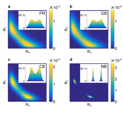
Figure 2: Stationary distribution of protein numbers, shown in the range $0\leq N_{\rm X},N_{\rm Y}\leq 700$ on a linear scale on both axes. (a) FM: Full model describing the mRNA and protein populations; (b) GB: protein-only model with geometrically distributed bursts; (c) CB: protein-only model with constant bursts; and (d) NB: protein-only model without bursts.

Diffusion approximation of the GB model. The evolution of the protein population in the GB model is described by a master equation (Supplementary Information). Solving master equations mathematically is however difficult and mostly limited to linear dynamics ^{28; 24}. The only realistic way forward for a theoretical analysis is often the so-called diffusion approximation.

In the diffusion approximation, the discrete-molecule process is approximated by a Gaussian process for continuous concentrations—numbers of the different types of molecules normalized by a typical population scale. The Gaussian process satisfies a diffusion equation (the Fokker–Planck equation) ^{29; 30}. Based on these methods, it is often possible to calculate or approximate the stationary behaviour and switching times of model gene networks. For existing studies in the context of toggle switches see ^{11; 13; 12}.

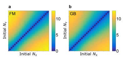
Figure 3: Mean first switching time as a function of the initial protein numbers ($0\leq N_{\rm X},N_{\rm Y}\leq 700$, shown on a linear scale). (a) FM: Full model; (b) GB model.

Deriving the diffusion approximation of the GB model requires modest modifications to the standard Kramers–Moyal expansion ^{29; 30}. These modifications are necessary to account for the randomness induced by the geometrically distributed burst size. Details of the derivation can be found in the Supplementary Information, we here only report the final outcome. The expansion results in two coupled Itō stochastic differential equations for the concentrations $x_{t}=N_{\rm X}(t)/K$ and $y_{t}=N_{\rm Y}(t)/K$. These are valid in the limit of large but finite populations ³¹ and of the form

$$dx_{t}={} v(x_{t},y_{t})dt+\sqrt{D(x_{t},y_{t})}dW_{t}^{(x)},$$ (1a)

$$dy_{t}={} v(y_{t},x_{t})dt+\sqrt{D(y_{t},x_{t})}dW_{t}^{(y)},$$ (1b)

with drift $v$ and diffusion $D$ given by

$$v(w,z):={} B\left(r_{0}+\frac{r}{1+z^{n}}\right)-{\gamma_{0}}w,$$ (2a)

$$D(w,z):={} \frac{B}{K}\left[\left(2B+1\right)\left(r_{0}+\frac{r}{1+z^{n}}\right)+\frac{\gamma_{0}}{B}w\right].$$ (2b)

The quantities $dW_{t}^{(x)}$ and $dW_{t}^{(y)}$ represent independent Wiener processes.

The diffusion approximation can only be expected to be accurate when molecule numbers are large so that the concentations $x_{t}$ and $y_{t}$ are effectively continuous. In principle, a similar analysis can also be applied to the master equations of the full model. In the FM mRNA numbers are rather small though (typically $<5$, see Supplementary Information), so the Gaussian approximation does not capture the statistics of the intrinsic noise faithfully. Similarly further analysis of the CB and NB models can be carried out based on the diffusion approximation. Given that CB and NB models fail to reproduce the behaviour of the FM, these results are relegated to the Supplementary Information.

Results from simulating the Gaussian process of equations (1) are shown in Fig. 4. While the data for the stationary distribution (Fig. 4a) looks similar to that of the full model (Fig. 2a), noticeable discrepancies are manifest in the mean first switching times (compare Fig. 4b and Fig. 3a). In Fig. 4c and d, we show the differences between simulation outcomes of the full model and those of the diffusion approximation of the GB model. Although the GB model itself approximates the full model well (Figs. 2 and 3), we conclude that the diffusion approximation fails to capture the relevant model outcomes.

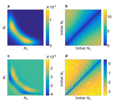
Figure 4: Diffusion approximation of the protein-only model with geometrically distributed random bursts (GB); (a) Stationary distribution as a function of the protein numbers; (b) Mean first switching time (MFST) as a function of the initial protein numbers, in the unit of cell cycles; (c) Net deviation of the stationary distribution from the full model; (d) Net deviation of the MFST from the FM. All axes show the range $0\leq N_{\rm X},N_{\rm Y}\leq 700$ on linear scales.

Constructing a mesoscopic piecewise deterministic Markov process. We have seen that the diffusion approximation of the GB model fails to reproduce the statistics of the full model. This underlines the need to construct coarse-grained models directly from the full model and without the intermediate step of a protein-only dynamics. We now proceed to introduce such a model. As before we describe protein concentrations by continuous variables, $x$ and $y$. The mRNA dynamics are captured by introducing three ‘states’: The $0$-state describes phases in which no mRNA is present. In the X-state there is one mRNA of type X and protein X is generated with rate $\gamma b$. The quantity $b=B/K$ is the mean burst size in the unit of protein concentration. No proteins of type Y are produced in the X-state. Similarly, in the Y-state protein Y is generated with rate $\gamma b$. Both types of protein are subject to natural degradation with rate $\gamma_{0}$ in any of the three states.

This is described by the following deterministic differential equations:

0-state: $$\quad\dot{x}=-\gamma_{0}x\quad\text{and}\quad\dot{y}=-\gamma_{0}y,$$ (3a)

X-state: $$\quad\dot{x}=\gamma b-\gamma_{0}x\quad\text{and}\quad\dot{y}=-\gamma_{0}y,$$ (3b)

Y-state: $$\quad\dot{x}=-\gamma_{0}x\quad\text{and}\quad\dot{y}=\gamma b-\gamma_{0}y.$$ (3c)

The rates with which the system transits between the states are based on the dynamics of the FM:

$$\text{0-state}\xrightarrow{H_{\text{}}\left(Ky\right)}{} \text{X-state, }~{}~{}~{}~{}~{}\text{X-state}\xrightarrow{\gamma}\text{0-state},$$

$$\text{0-state}\xrightarrow{H_{\text{}}\left(Kx\right)}{} \text{Y-state, }~{}~{}~{}~{}~{}\text{Y-state}\xrightarrow{\gamma}\text{0-state}.$$ (4)

No transitions occur directly between the X and Y states. The kinetic scheme is illustrated in Fig. 1d.

The stochasticity and discreteness of the mRNA populations is reflected in the random transitioning between the 0-, X- and Y-states. Between these Markovian events the protein concentrations evolve deterministically. We will refer to this model as the piecewise deterministic Markov process (PDMP).

Notably, at most one mRNA molecule of either type can be present in PDMP at any time. Although the model can be generalised to allow more than one mRNA molecule, the analysis below shows that the lowest-order approximation is sufficient to capture the relevant fluctuations of the mRNA dynamics.

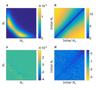
Figure 5: PDMP approximation. (a) Stationary distribution; (b) Mean first switching time in the unit of cell cycles as a function of initial protein numbers. (c) Net deviation of the stationary distribution from the full model; (d) Net deviation of the MFST of the PDMP model from the FM. All axes are on linear scales and show the range $0\leq N_{\rm X},N_{\rm Y}\leq 700$.

The PDMP approximation outperforms the diffusion approximation of the GB model. As in the GB model, we work in the limit of infinitely fast degrading mRNA ($\gamma\rightarrow\infty$). Simulations of the PDMP model in this limit can be carried out using a minor modification of a previously proposed algorithm¹⁵. We measure the stationary distribution of the PDMP model and the mean first switching times for different initial protein numbers. Results are shown in Fig. 5a and b, and we compare the outcome against that of the full model in Fig. 5c and d.

The simulation data indicate that the PDMP approximation outperforms the diffusion approximation of the GB model, and it provides a more faithful approximation to the FM. This is because the diffusion approximation introduces Gaussian noise. It retains some information about the variance of protein production and degradation, but it does not capture the geometrically distributed burst sizes in the GB model well enough. The PDMP approximation, on the other hand, models exponentially distributed bursts in protein concentration. The exponential distribution in the PDMP model is the analogue of the geometric distribution in the discrete-molecule GB model. While the PDMP model is an approximation as well, it retains the typical characteristics of the stationary distribution and switching times of the original model. At the same time the PDMP model is suitable for further mathematical analysis (see below).

When does the PDMP outperform the diffusion approximation? We now investigate the robustness of these findings. In Fig. 6 we vary two essential parameters, the mean burst size $B$, and the population scale $K$, while keeping the other parameters fixed. We measure the Jensen–Shannon distance ^{32; 33} between the resulting stationary distributions of the PDMP and that of the the full model. Data is shown in Fig. 6a and c. We also compare the mean first switching times starting from one of the stable modes, see Fig. 6b and d. The figure also shows results from the diffusion approximation of the GB model.

Results indicate that PDMP model outperforms the diffusion approximation of the GB model for mean burst sizes of $B\gtrsim 5$. We conclude that the bursting noise has to be considered in this biologically relevant regime ²⁴. The PDMP model incorporates only the bursting noise and neglects the demographic noise from random degradation of the proteins. The strength of this demographic noise is proportional to $1/\sqrt{K}$. The results in Fig. 6 c and d indicate that the difference in describing intrinsic noise propagates to physical observables even when the noise is weak ($K\approx 1000$ for fixed $B=30$).

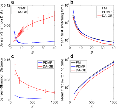
Figure 6: Performance of the PDMP model and the diffusion approximation of the GB model (DA-GB). (a) Jensen–Shanon distance between the stationary distribution PDMP (and DA-GB) and the stationary distribution of the FM; (b) Mean first switching time for varying value of $B$ at fixed $K=200$; (c-d) Similar to (a-b) but now varying $K$ at fixed $B=30$.

Analytic investigation of the PDMP process. The simplicity of the PDMP approach allows us to proceed with a mathematical analysis. We here only outline the main steps, further details are reported in the Supplementary Information. We denote the probability density that the system is in the $0$-state and with protein densities $x,y$ at time $t$ by $p_{\text{0}}(x,y,t)$. Similarly we write $p_{\text{X}}(x,y,t)$ and $p_{\text{Y}}(x,y,t)$ when the system is in the X- or Y-states. The evolution of these distributions then follows the forward equation

$$\frac{\partial}{\partial t}\left[\begin{array}[]{c}p_{\text{0}}\\ p_{\text{X}}\\ p_{\text{Y}}\end{array}\right]=\left(L^{\dagger}_{d}+L^{\dagger}_{\text{s}}\right)\left[\begin{array}[]{c}p_{\text{0}}\\ p_{\text{X}}\\ p_{\text{Y}}\end{array}\right],$$ (5)

where $L^{\dagger}_{d}$ and $L^{\dagger}_{s}$ drive the deterministic flow and the random switching between states respectively. These operators are of the form

$$L^{\dagger}_{d}:={} \left[\begin{array}[]{ccc}\left(L^{\dagger}_{d}\right)_{11}&0&0\\ 0&\left(L^{\dagger}_{d}\right)_{22}&0\\ 0&0&\left(L^{\dagger}_{d}\right)_{33}\end{array}\right],$$ (6d)

$$L^{\dagger}_{s}:={} \left[\begin{array}[]{ccc}-H_{\text{}}(Kx)-H_{\text{}}(Ky)&\gamma&\gamma\\ H_{\text{}}(Ky)&-\gamma&0\\ H_{\text{}}(Kx)&0&-\gamma\end{array}\right],$$ (6h)

with

$$\left(L^{\dagger}_{d}\right)_{11}:={} \gamma_{0}\partial_{x}\left(x\right)+\gamma_{0}\partial_{y}\left(y\right),$$ (7a)

$$\left(L^{\dagger}_{d}\right)_{22}:={} \partial_{x}\left(-\gamma b+\gamma_{0}x\right)+\gamma_{0}\partial_{y}\left(y\right),$$ (7b)

$$\left(L^{\dagger}_{d}\right)_{33}:={} \gamma_{0}\partial_{x}\left(x\right)+\partial_{y}\left(-\gamma b+\gamma_{0}y\right).$$ (7c)

The differential operators $\partial_{x}$ and $\partial_{y}$ act on all that follows to their right, including the probability densities $p_{0},p_{\text{X}}$ and $p_{\text{Y}}$ outside the matrix notation in equations (5) and (6).

The PDMP approximation applies in the limit $\gamma\rightarrow\infty$, i.e., fast return into the 0-state. The resident time in the X- and Y-states is exponentially distributed and scales as $\gamma^{-1}$. It formally tends to zero as $\gamma\to\infty$. On the other hand the translation rate $\gamma B$ tends to infinity in this limit. Combining the limiting behaviours of resident time and translation rate results in an exponentially distributed increment of protein concentration in each cycle of switching from the 0-state to the X- or Y-state, and then returning to the 0-state. As a consequence the PDMP converges to previously proposed continuous-state bursting models ^{14; 15; 18} in the limit $\gamma\rightarrow\infty$, and $p_{\text{0}}(x,y,t)$ satisfies

$$\partial_{t}p_{0}={} \partial_{x}\left(\gamma_{0}xp_{0}\right)+\partial_{y}\left(\gamma_{0}yp_{0}\right)-\left[H_{\text{}}(Kx)+H_{\text{}}(Ky)\right]p_{0}$$

$$+H_{\text{}}(Ky)\int_{0}^{x}\frac{1}{b}e^{-\frac{x-x^{\prime}}{b}}p_{0}\left(x^{\prime},y,t\right)dx^{\prime}$$

$$+H_{\text{}}(Kx)\int_{0}^{y}\frac{1}{b}e^{-\frac{y-y^{\prime}}{b}}p_{0}\left(x,y^{\prime},t\right)dy^{\prime},$$ (8)

as detailed in the Supplementary Information.

Analytic investigation of the mean first switching time. One of the strengths of the PDMP formulation (equations (5) and (6)) is the relative ease with which mean first switching times can be obtained. We first proceed by computing mean escape time from an arbitrary open domain $\Omega$. The mean first switching time can be calculated by setting $\Omega=\left\{(x,y):x<y\right\}$, recognising that the process can only exit this domain by crossing the boundary $x=y$.

Suppose, the system is initially at $(x,y)\in\Omega$, and in state $\text{Z}\in\left\{0,\text{X},\text{Y}\right\}$. We write $T_{\text{Z}}\left(x,y\right)$ for the mean first time at which the process exits the domain $\Omega$. The quantities $T_{\text{Z}}$ then satisfy the following backward equation ^{29; 30}

$$-\left[\begin{array}[]{c}1\\ 1\\ 1\end{array}\right]=\left(L_{d}+L_{\text{s}}\right)\left[\begin{array}[]{c}T_{0}(x,y)\\ T_{\text{X}}(x,y)\\ T_{\text{Y}}(x,y)\end{array}\right],$$ (9)

where $L_{d}$ and $L_{s}$ are adjoint to the operators in equations (6). They are given by

$$L_{d}:={} \left[\begin{array}[]{ccc}\left(L_{d}\right)_{11}&0&0\\ 0&\left(L_{d}\right)_{22}&0\\ 0&0&\left(L_{d}\right)_{33}\end{array}\right],$$ (10d)

$$L_{s}:={} \left[\begin{array}[]{ccc}-H_{\text{}}(Kx)-H_{\text{}}(Ky)&H_{\text{}}(Ky)&H_{\text{}}(Kx)\\ \gamma&-\gamma&0\\ \gamma&0&-\gamma\end{array}\right]$$ (10h)

with

$$\left(L_{d}\right)_{11}={} -\gamma_{0}x\partial_{x}-\gamma_{0}y\partial_{y},$$ (11a)

$$\left(L_{d}\right)_{22}={} \left(\gamma b-\gamma_{0}x\right)\partial_{x}-\gamma_{0}\left(y\right)\partial_{y},$$ (11b)

$$\left(L_{d}\right)_{33}={} -\gamma_{0}x\partial_{x}+\left(\gamma b-\gamma_{0}y\right)\partial_{y}.$$ (11c)

In the infinitely-fast degrading mRNA limit ($\gamma\rightarrow\infty$), and using appropriate boundary conditions (Supplementary Information) we arrive at

$$-1={} \left[-\gamma_{0}x\partial_{x}-\gamma_{0}y\partial_{y}-H(Kx)-H(Ky)\right]T_{0}\left(x,y\right)$$

$$+H(Ky)\int_{x}^{y}\frac{e^{-\frac{x^{\prime}-x}{b}}}{b}T_{0}\left(x^{\prime},y\right)dx^{\prime}$$

$$+H(Kx)\int_{y}^{\infty}\frac{e^{-\frac{y^{\prime}-y}{b}}}{b}T_{0}\left(x,y^{\prime}\right)dx^{\prime}.$$ (12)

This is the adjoint equation²⁹ of the expression in equation (8) on the open domain $\Omega$. Equation (12) is solved by a finite difference method, noting that it is self-consistent and no boundary condition needs to be specified. The solution is shown in Fig. 7, and reproduces the simulation outcome of the FM well.

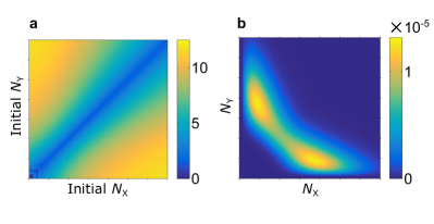
Figure 7: Theoretical prediction of the PDMP model. (a) Mean first passage time as a function of initial protein numbers, calculated from the backward equation (12); (b) Stationary distribution of protein numbers calculated from the WKB method. Axes of both panels show the range $0\leq N_{\rm X}(0),N_{\rm Y}(0)\leq 700$ on linear scales.

We remark that equation (12) is only valid for the half-plane $\Omega$. A detailed discussion can be found in the Supplementary Information.

Analytic investigation of the weak-noise limit. The analytical calculation of the stationary distributions of the PDMP model can be pursued further using the so-called Wentzel-Kramers-Brillouin (WKB) method. This technique is based on the ansatz

$$p_{\rm stat}\left(x,y\right)=\exp\left[-\frac{1}{b}\sum_{\ell=0}^{\infty}b^{\ell}S_{\ell}\left(x,y\right)\right],$$ (13)

where $b=B/K\ll 1$. One proceeds by considering $\left(L_{d}^{\dagger}+L_{s}^{\dagger}\right)p_{\rm stat}(x,y)=0$ order-by-order in $b$. To leading order we find the Hamilton–Jacobi equation

$$0={} \left[\gamma_{0}x-Bh\left(y\right)\right)]\partial_{x}S_{0}+\left[\gamma_{0}y-Bh\left(x\right)\right]\partial_{y}S_{0}$$

$$+\left[\gamma_{0}x+\gamma_{0}y-Bh\left(x\right)-Bh\left(y\right)\right]\left(\partial_{x}S_{0}\right)\left(\partial_{y}S_{0}\right)$$

$$+\gamma_{0}x\left(\partial_{x}S_{0}\right)^{2}+\gamma_{0}y\left(\partial_{y}S_{0}\right)^{2}$$

$$+\gamma_{0}x\left(\partial_{x}S_{0}\right)^{2}\left(\partial_{y}S_{0}\right)+\gamma_{0}y\left(\partial_{x}S_{0}\right)\left(\partial_{y}S_{0}\right)^{2},$$ (14)

where $h(z):=H(Kz)/K$. This equation is then numerically solved using the algorithm of Heymann and Vanden–Eijnden ³⁴. Results are shown in Fig. 8. Even though this only provides a first-order approximation and despite the fact that we have used $b=0.15$ (which is not very small) we obtain a reasonable agreement with the stationary distribution in Fig. 5a.

For completeness we have also carried out a WKB analysis of the diffusion approximation of the GB, CB and NB models. These are presented in the Supplementary Information.

The leading order function $S_{0}\left(x,y\right)$ is the so-called ‘rate function’ which quantifies the rare-event statistics of the process in the weak-noise limit $b\ll 1$ ^{35; 36}. Several studies have suggested that $S_{0}\left(x,y\right)$ is a suitable candidate for a ‘landscape’ of the non-equilibrium random processes in models of gene regulatory networks^{11; 10; 16; 17; 9}. The Hamilton–Jacobi equation (14) contains cubic terms such as $\left(\partial_{x}S_{0}\right)^{2}\left(\partial_{y}S_{0}\right)$, while diffusion equations are quadratic in derivatives of $S_{0}$. This illustrates the fundamental difference between the statistics of intrinsic noise in the diffusion approximation and the bursting noise in PDMP. Further more rigorous mathematical investigations into these differences would be very welcome in our view.

Figure 8: Rate functions $S_{0}$ as functions of the protein numbers $0\leq N_{\rm X},N_{\rm Y}\leq 700$ on a linear scale. (a) PDMP model; (b) Diffusion approximation of the GB model.

We compare the functions $S_{0}$ of the PDMP and the diffusion approximation of the GB model in Fig. 8. One observes a much ‘shallower’ rate function in the PMDP model, especially at larger protein numbers ($N_{\rm X},N_{\rm Y}\approx 700$). This is due to the long tails in the exponential bursting kernel of the PDMP model, which are not present in the diffusion approximation of the GB model. Such a fat-tail bursting kernel enhances the probability for the system to evolve to high protein concentrations. We identify this as the origin of the qualitatively distinct rare-event statistics in the two models.

Effects of bursting noise in a multi-switch network. Recently, multi-switch systems have gained interest^{13; 21; 37}. A schematic diagram of the three-way switch network proposed by ¹³ is shown in Fig. 9a. It is obtained from the classical toggle switch network by including a self-enhancing autoregulation. Our computational and mathematical setup requires only minor modifications to include generalisation to this case. Specifically, we replace the earlier Hill functions by

$$G(N_{\rm X},N_{\rm Y})={} q_{0}\left(1+\frac{r_{1}}{(N_{\rm X}/K_{1})^{n_{1}}+1}\right)$$

$$\times\left(1+\frac{r_{2}}{(N_{\rm Y}/K_{2})^{n_{2}}+1}\right),$$ (15)

with parameters¹³ $q_{0}=4$, $r_{1}=-4/5$, $r_{2}=7/3$, $n_{1}=3$, $n_{2}=1$, $K_{1}=160$, and $K_{2}=320$. The rest of the parameters follows Table 1. The negative value of $r_{1}$ reflects the positive autoregulation. To evaluate the effects of bursting noise on this multi-switch model, we consider again the full model, the diffusion approximation of the GB model, as well as the CB and NB models of the extended network.

Fig. 9 displays the stationary distribution to illustrate the effects of the bursting noise in the multi-switch network. The model without bursts (NB, panel f) has a stationary distribution consisting of three modes, as reported earlier¹³. Inclusion of constant bursts (CB, panel e) diversifies the protein expression and reduces the stability of the mode located at $N_{\rm X}=N_{\rm Y}\approx 230$. In the full model (panel b) there is no discernible concentration of probability in the symmetric mode, hence the three-way switching capability appears to be absent. We also notice that the saddle of the distribution in the FM is located at a state with much lower number of proteins compared to the NB and CB models. The most likely switching path ⁹ from one of the asymmetric modes to the other will differ significantly between the different variants of the model. The diffusion approximation of the GB model (panel c) does not capture the outcome of the FM either. Overall these findings confirm again that the inclusion of bursty noise statistics has significant effects on the model outcome. Finally, we observe in Fig. 9d that the PDMP model approximates the full model of the three-way switch well. We conclude that randomly distributed burst sizes are again the predominant form of intrinsic noise in the multi-switch network.

II Discussion and conclusion

Explicitly including mRNA dynamics in gene regulatory models inevitably introduces more complexity. We have quantitatively studied the effects of bursting noise ¹ in a biologically relevant regime or the model organism E. coli. To our knowledge, this is one of the first which attempts to build a rigorous connection between existing individual-based models^{3; 8; 9; 10} and more coarse-grained models^{11; 12; 14; 15}. Results of our simulations indicate that the bursting statistics of transcription and translation are essential ingredients of models of gene regulation. Coarse grained models need to account for bursting to retain correct statistics of noise-driven phenomena such as the switching between different dynamic attractors.

The implications of our observations are relevant to the abstract modelling of regulatory networks in different ways. We are now in a better position to address our opening question, and to say how noise propagates between different levels of modelling. Perhaps more importantly, our study may ultimately help to decide what level of modelling is most appropriate to study gene regulatory circuits computationally. The answer will of course depend on the question in the focus of the investigation. We have examined different levels of coarse graining, and we have identified the steps in these reduction procedures at which significant alternations to different model outcomes are introduced.

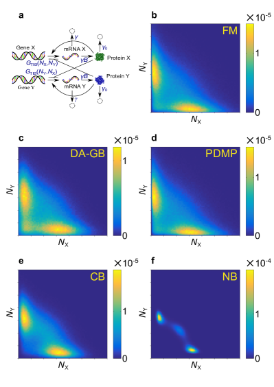
Figure 9: (a) Schematic diagram illustrating the network of the three-way switch, remaining panels show stationary distribution of protein numbers in the range $0\leq N_{X},N_{Y}\leq 700$ on linear scale. (b) Full model; (c) Diffusion approximation of the GB model; (d) PDMP approximation; (e) CB model; and (f)NB model.

Systematically choosing a suitable level of coarse-graining also facilitates the mathematical analysis of regulatory networks. The high dimensionality of full regulatory network effectively makes them intractable. Model reduction is needed to make progress, and our analysis demonstrates that the PDMP formulation is a powerful way forward, and that it can be more suitable than the conventional diffusion approximation. The PDMP model explicitly retains the bursting noise originating from the mRNA dynamics. Even though it effectively disregards the demographic noise from random degradation of the proteins, it delivers accurate predictions for stationary distributions and switching times.

As another strength, the PDMP formulation can relatively easily be generalised to accommodate more complex reactions. For example, in the Enterobacteria phage $\lambda$ switch it is not the monomer of the synthesized proteins which acts as the repressor to regulate transcription, but instead their dimer. Modelling these processes requires the inclusion of dimerization further downstream after transcription and translation ^{7; 10}. Preliminary results not shown here reveal that the PDMP approximates such dynamics well.

The fact that the piecewise deterministic Markov process is successful in approximating the full model opens a relatively new type of modelling paradigm. We acknowledge that we are not the first to propose this ^{38; 39; 40; 41; 28}. Our contribution consists in a first analytical treatment of PDMP models and in an systematic embedding into a wider landscape of modelling approaches. The bursting phenomenon is ubiquitous whenever there is a separation of time scales between the source and the product of a biological process. These are mRNA and protein in models of gene regulation, but we expect that these ideas can be applied to other biological problems with similar time-scale separation.

III Methods

Sample paths of the individual-based processes (FM, CB, NB, and GB) are generated using the standard Gillespie algorithm ^{26; 27}. The PDMP process is simulated using the algorithm discussed by Bokes et al¹⁵. Simulations of the stochastic differential equations resulting from the diffusion approximation are performed with a standard Euler–Maruyama scheme. The geometric minimum action method³⁴ is implemented using MATLAB R2010a, as is the finite-difference scheme to solve the backward equation (12). Further details can be found in the Supplementary Information.

IV Acknowledgement

The authors acknowledge supported by the Engineering and Physical Sciences Research Council EPSRC (UK) (grant reference EP/K037145/1). We thank Peter Ashcroft, Luis Fernandez–Lafuerza, Louise Dyson, and Charlie Doering for fruitful discussions.

V Author contributions

Y.T.L. conceived the study, performed analytical calculations and numerical simulations, prepared the figures. T.G. provided general direction of the study, confirming analytical calculations. Both authors wrote the manuscript.

VI Additional information

Supplementary Information accompanies this manuscript.

Competing financial interests: The authors declare no competing financial interests.

References

- (1) Kaern, M., Elston, T. C., Blake, W. J. & Collins, J. J. Stochasticity in gene expression: From theories to phenotypes. Nat. Rev. Genet. 6, 451–464 (2005).
- (2) Thattai, M. & van Oudenaarden, A. Intrinsic noise in gene regulatory networks. Proc. Natl. Acad. Sci. USA 98, 8614–8619 (2001).
- (3) Walczak, A. M., Mugler, A. & Wiggins, C. H. Analytic methods for modeling stochastic regulatory networks. Methods Mol. Biol. 880, 273–322 (2012).
- (4) Thattai, M. & van Oudenaarden, A. Stochastic gene expression in fluctuating environments. Genetics 167, 523–530 (2004).
- (5) Acar, M., Mettetal, J. T., & van Oudenaarden, A. Stochastic switching as a survival strategy in fluctuating environments. Nat. Genet. 40, 471–475 (2008).
- (6) Roberts, E., Magis, A., Ortiz, J. O., Baumeister, W. & Luthey-Schulten, Z. Noise contributions in an inducible genetic switch: A whole-cell simulation study. PLoS Comput. Biol. 7, e1002010 (2011).
- (7) Arkin, A., Ross, J. & McAdams, H. H. Stochastic kinetic analysis of developmental pathway bifurcation in phage -infected escherichia coli cells. Genetics 149, 1633–1648 (1998).
- (8) Walczak, A. M., Sasai, M. & Wolynes, P. G. Self-consistent proteomic field theory of stochastic gene switches. Biophys. J. 88, 828–850 (2005).
- (9) Roma, D. M., O’Flanagan, R. A., Ruckenstein, A. E., Sengupta, A. M. & Mukhopadhyay, R. Optimal path to epigenetic switching. Phys. Rev. E 71, 011902 (2005).
- (10) Warren, P. B. & ten Wolde, P. R. Chemical models of genetic toggle switches. J. Phys. Chem. B 109, 6812–6823 (2005).
- (11) Wang, J., Zhang, K., Xu, L. & Wang, E. Quantifying the waddington landscape and biological paths for development and differentiation. Proc. Natl. Acad. Sci. USA 108, 8257–8262 (2011).
- (12) Wang, J., Xu, L., Wang, E. & Huang, S. The potential landscape of genetic circuits imposes the arrow of time in stem cell differentiation. Biophys. J. 99, 29–39 (2010).
- (13) Lu, M. Y., Onuchic, J. & Ben-Jacob, E. Construction of an effective landscape for multistate genetic switches. Phys. Rev. Lett. 113, 5 (2014).
- (14) Friedman, N., Cai, L., Xie & X. S. Linking stochastic dynamics to population distribution: An analytical framework of gene expression. Phys. Rev. Lett. 97, 168302 (2006).
- (15) Bokes, P., King, J., Wood, A. A. & Loose, M. Transcriptional bursting diversifies the behaviour of a toggle switch: Hybrid simulation of stochastic gene expression. Bull. Math. Biol. 75, 351–371 (2013).
- (16) Strasser, M., Theis, F. J. & Marr, C. Stability and multiattractor dynamics of a toggle switch based on a two-stage model of stochastic gene expression. Biophys. J. 102, 19–29 (2012).
- (17) Assaf, M., Roberts, E. & Luthey-Schulten, Z. Determining the stability of genetic switches: Explicitly accounting for mrna noise. Phys. Rev. Lett. 106, 248102 (2011).
- (18) Cai, L., Friedman, N. & Xie, X. S. Stochastic protein expression in individual cells at the single molecule level. Nature 440, 358–362 (2006).
- (19) Gardner, T. S., Cantor, C. R. & Collins, J. J. Construction of a genetic toggle switch in escherichia coli. Nature 403, 339–342 (2000).
- (20) Wang, J. W., Zhang, J. J., Yuan, Z. J. & Zhou, T. S. Noise-induced switches in network systems of the genetic toggle switch. BMC Syst. Biol. 1, 14 (2007).
- (21) Lu, M. et al. Tristability in cancer-associated microRAN-TF chimera toggle switch. J. Phys. Chem. B 117, 13164–13174 (2013).
- (22) Taniguchi, Y. et al. Quantifying e-coli proteome and transcriptome with single-molecule sensitivity in single cells. Science 329, 533–538 (2010).
- (23) Kobayashi, H. et al. Programmable cells: Interfacing natural and engineered gene networks. Proc. Natl. Acad. Sci. USA 101, 8414–8419 (2004).
- (24) Shahrezaei, V. & Swain, P. S. Analytical distributions for stochastic gene expression. Proc. Natl. Acad. Sci. USA 105, 17256–17261 (2008).
- (25) Raj, A. & van Oudenaarden, A. Nature, nurture, or chance: Stochastic gene expression and its consequences. Cell 135, 216–226 (2008).
- (26) Schwartz, R. Biological modeling and simulation : a survey of practical models, algorithms, and numerical methods. Cambridge, MA: MIT Press (2008).
- (27) Gillespie, D. T. Exact stochastic simulation of coupled chemical-reactions. J. Phys. Chem. 81, 2340–2361 (1977).
- (28) Kumar, N., Platini, T. & Kulkarni, R. V. Exact distributions for stochastic gene expression models with bursting and feedback. Phys. Rev. Lett. 113, 5 (2014).
- (29) van Kampen, N. G. Stochastic Processes in Physics and Chemistry. Amsterdam: Elsevier Science B.V. (2007).
- (30) Gardiner, C. W. Handbook of Stochastic Methods. Springer, New York (2009).
- (31) Kurtz, T. G. Limit theorems for sequences of jump Markov processes approximating ordinary differential processes. J. Appl. Probab. 8, 344–356 (1971).
- (32) Lin, J. H. Divergence measures based on the shannon entropy. IEEE Trans. Inf. Theory 37, 145–151 (1991).
- (33) Endres, D. M. & Schindelin, J. E. A new metric for probability distributions. IEEE Trans. Inf. Theory 49, 1858–1860 (2003).
- (34) Heymann, M. & Vanden-Eijnden, E. The geometric minimum action method: A least action principle on the space of curves. Comm. Pure Appl. Math. 61, 1052–1117 (2008).
- (35) Freidlin, M. I. & Wentzell, A. D. Random Perturbations of Dynamical Systems. New York: Springer-Verlag (2012).
- (36) Zhou, J. X., Aliyu, M. D. S., Aurell, E. & Huang, S. Quasi-potential landscape in complex multi-stable systems. J. R. Soc. Interface 9, 3539–3553 (2012).
- (37) Guantes, R. & Poyatos, J. F. Multistable decision switches for flexible control of epigenetic differentiation. PLoS Comput. Biol. 4 e1000235. (2008).
- (38) Hasty, J., Pradines, J., Dolnik, M. & Collins, J. J. Noise-based switches and amplifiers for gene expression. Proc. Natl. Acad. Sci. USA 97, 2075–2080 (2000).
- (39) Zeiser, S., Franz, U., Wittich, O. & Liebscher, V. Simulation of genetic networks modelled by piecewise deterministic markov processes. IET Syst. Biol. 2, 113–135 (2008).
- (40) Zeiser, S., Franz, U. & Liebscher, V. Autocatalytic genetic networks modeled by piecewise-deterministic markov processes. J. Math. Biol. 60, 207–246 (2010).
- (41) Huang, G. R., Saakian, D. B., Rozanova, O., Yu, J. L. & Hu, C. K. Exact solution of master equation with gaussian and compound poisson noises. J. Stat. Mech. P11033 (2014).