Connecting strongly correlated superfluids by a quantum point contact
Abstract
Point contacts provide simple connections between macroscopic particle reservoirs. In electric circuits, strong links between metals, semiconductors or superconductors have applications for fundamental condensed-matter physics as well as quantum information processing. However for complex, strongly correlated materials, links have been largely restricted to weak tunnel junctions. Here we study resonantly interacting Fermi gases connected by a tunable, ballistic quantum point contact, finding a non-linear current-bias relation. At low temperature, our observations agree quantitatively with a theoretical model in which the current originates from multiple Andreev reflections. In a wide contact geometry, the competition between superfluidity and thermally activated transport leads to a conductance minimum. Our system offers a controllable platform for the study of mesoscopic devices based on strongly interacting matter.
The effect of strong interactions between the constituents of a quantum many-body system is at the origin of several challenging questions in physics. Whilst the ground states of strongly interacting systems are increasingly better understood Leggett:2006aa , the properties out of equilibrium and at finite temperature often remain puzzling, as these are determined by the excitations above the ground state. In laboratory experiments, strongly interacting systems are found in certain materials, as well as in quantum fluids and gases Leggett:2006aa . In solid-state systems, a conceptually simple and clean approach to probe non-equilibrium physics is provided by transport measurements through the well-defined geometry of a quantum point contact (QPC) Post:1994aa ; Scheer:1997aa ; Fischer:2007aa . Yet, the technical hurdles to realise a controlled QPC between strongly correlated materials pose a big challenge. Ultra-cold atomic Fermi gases in the vicinity of a Feshbach resonance, the so-called unitary regime, provide an alternative route to study correlated systems Zwerger:2011aa . Superfluidity has been established at low temperature Zwierlein:2005ab , but the finite- temperature properties are only partially understood Nascimbene:2011aa ; Ku:2012aa ; Sagi:2015aa , a situation similar to the field of strongly correlated materials.
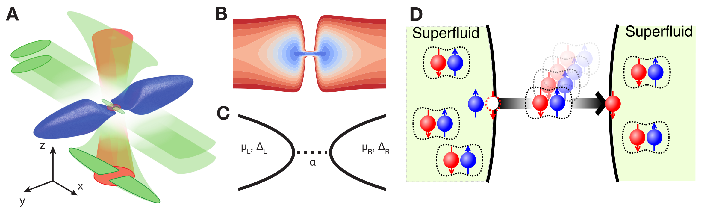
Recent progresses in the manipulation of cold atomic gases have allowed to create a mesoscopic device featuring quantised conductance between two reservoirs in the non-interacting regime Krinner:2015aa . We use this technique to create a QPC in a strongly interacting Fermi gas consisting of 6Li atoms in each of the two lowest hyperfine states, in a magnetic field of 832 G, where the interaction strength diverges due to a broad Feshbach resonance. The atoms form a strongly correlated superfluid, with a pairing gap larger than the chemical potential Zwerger:2011aa . Typical temperatures in the cloud are nK at a chemical potential of . The setup is presented in Figure 1A materialsandmethods . The QPC is characterised by transverse trapping frequencies of and kHz in - and -direction. An optical attractive ”gate” potential is used to tune the chemical potential and the number of channels in the QPC (see Figure 1B) materialsandmethods . We prepare two atomic clouds (reservoirs) with an atom number difference while blocking transport through the QPC with a repulsive laser beam. This results in a chemical potential bias between the two reservoirs , with the Fermi temperature and the function derived from the equation of state (EoS) of the trapped Fermi gas at unitarity Ku:2012aa ; materialsandmethods .
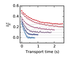
We open the QPC and measure as a function of time . Figure 2A presents this evolution for various strengths of the gate potential . We observe that the decays from its initial value to zero over a time scale of 0.5 to 1.5s. The shape of the decay curves deviates from an exponential and is a direct manifestation of a non- linear relation between and the atom current.
We extract the numerical derivative of these data materialsandmethods , yielding the instantaneous current at a certain shown in Figure 2B. We normalise the current and bias by the strength of the pairing gap , using the known relation of with the chemical potential for the low temperature Fermi gas, , with Schirotzek:2008aa and Ku:2012aa ; Zurn:2013aa .
The current-bias characteristics in Figure 2B are strongly non- linear for all the choices of , featuring a very strong response at low bias. The high-bias regime approaches a linear dependance with a nonzero intercept on the current axis, marking an excess current that depends on the strength of the . The current is much larger than what is observed for non-interacting atoms Krinner:2015aa , as observed in earlier measurements on strongly interacting atoms in multimode channels Stadler:2012kx .
We model the experimental system as two superfluid reservoirs connected by a single particle hopping mechanism solely characterised by the transparency of the QPC (see Figure 2C) Blonder:1982aa ; Averin:1995aa ; Cuevas:1996aa ; Bolech:2004aa ; PhysRevB.71.024517 . This model excludes any finite size and geometry-dependent effects, which we think of as absorbed in . It is motivated by the large proximity effect in superfluids separated by a ballistic normal barrier Zagoskin:1998aa . Indeed, we expect a coherence length of m, where is the Fermi velocity, is Boltzmann’s constant and is the temperature of the gas. This is comparable to half the length of the channel (5.6 m), thus we approximate the channel with a point-like connection. Using a non-equilibrium Keldysh Green function technique Kamenev:2011aa with mean-field approximation materialsandmethods we compare theoretical current-bias curves with our data.
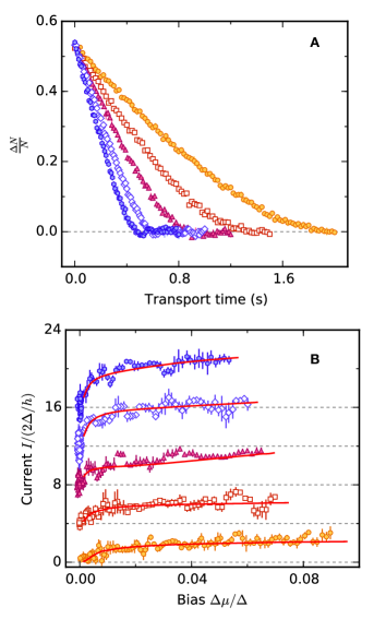
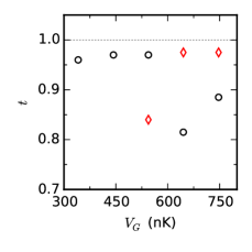
Since the pairing gap and the EoS of the unitary gas are known a priori, the only free parameter in our model is the transparency for each transverse mode in the QPC materialsandmethods . The solid lines in Figure 2B show the results with the best fits of . For the two lowest gate potentials we obtain good agreement with a single channel model, whereas for higher gate potentials three channels are required, in agreement with our reference measurement with a weakly interacting Fermi gas Krinner:2015aa .
The agreement between theory and experiment clarifies the microscopic origin of the current. Reflecting the strongly interacting nature of the system, we have . In this regime, a current flow is allowed via multiple coherent reflections of quasiparticles between superconducting reservoirs, i.e., multiple Andreev reflections, illustrated in Figure 1D Averin:1995aa . The gap for a single particle transfer can be bridged by the simultaneous, coherent transfer of pairs if , with a probability of order . As is seen in Figure 2B, the drop of current observed at low bias corresponds to Averin:1995aa , where the finite transparency suppresses the corresponding Andreev processes. In the very low bias regime, not resolved in the experiment, the DC current is exponentially suppressed and an oscillating current caused by the energy mismatch between the two reservoirs occurs. This averages to zero in the DC limit, and represents an AC Josephson current adding to the DC response materialsandmethods ; PhysRevLett.60.416 ; RevModPhys.74.741 ; Albiez:2005aa ; Ramanathan:2011aa ; LeBlanc:2011aa ; Jendrzejewski:2014aa .
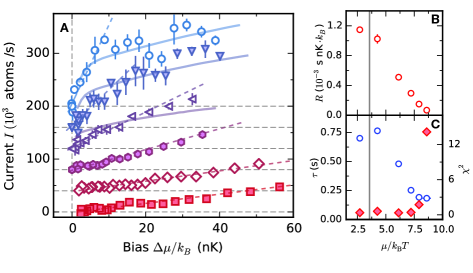
We now investigate the current-bias relation as a function of temperature, for a fixed gate potential nK. To this end, we introduce a controlled heating of both reservoirs before the transport is started, using variable amplitude parametric heating. With this method we explore a temperature range of 124-290 nK, from a deeply superfluid regime up to the superfluid-to-normal transition point. We measure the decay of particle imbalance with increasing temperature and observe a crossover towards exponential decay when temperature is above 145 nK. We extract the current- bias characteristic (Figure 3A) using the known finite-temperature EoS of the unitary Fermi gas Ku:2012aa ; materialsandmethods . With increasing temperature the non-linearity disappears and the current globally decreases. We interpret this as the disappearance of the superfluid contribution to transport as temperature is raised.
From these data, the differential resistance at low bias is estimated by fitting a line to the low bias region of the curve. The result is presented in Figure 3B, where the decrease in is clearly visible as temperature is decreased. We compare this to a model independent measure of the non-linearity of the characteristic provided by the parameter of an exponential fit to the entire decay curves materialsandmethods . This parameter, as well as the fitted timescale of the exponential decay tracks the measured differential resistance (Figure 3C).
While in the low temperature regime, non-linearity is captured by our mean- field model, the model fails to reproduce the resistance at high temperature, indicating a breakdown of the mean-field description. In particular, it predicts a resistance in the linear regime given by the non-interacting Landauer formula, while the resistance that we measure is one order of magnitude smaller. This constitutes an indirect evidence that the high temperature state of the gas is not a Fermi liquid, since Fermi liquid theory leads to the Landauer formula, setting the upper limit for the current carried by an ideal contact. One possible explanation is the presence of superfluid fluctuations, which are expected to be large close to Liu:2014aa . Indeed, it is known that a one-dimensional Fermi gas held between attractively interacting leads, a prototype of non-Fermi liquid system giamarchi:2003 , shows an enhanced conductance Maslov:1995aa ; Safi:1995aa ; PhysRevB.52.R8666 .
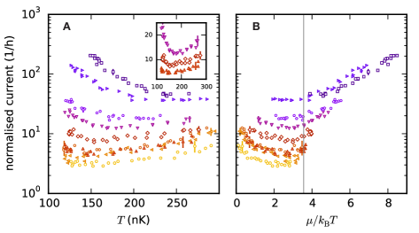
The physical picture emerging from these measurements relies on the finite- temperature properties of the reservoirs. Some of the intrinsic physics of the channel appears when the mode spacing in the QPC is comparable to the temperature range explored. In this situation, several modes are thermally populated Brantut:2013aa , enhancing transport for increasing temperature and competing with the subsequent reduction of the superfluid current. To show this, we decrease the confinement in the QPC along the direction to kHz and systematically measure the current at the largest bias as a function of temperature for various gate potential. The results are shown in Figure 4A where the current at high bias normalised to the bias is shown as a function of temperature for various gate potentials. In the linear response regime, this current-bias-ratio reduces to the differential conductance.
For large , we observe a decrease of the current with temperature over one order of magnitude. In this superfluid-dominated regime, the pairing gap is large compared to both temperature and level spacing in the QPC, analogous to the previous measurements. At low , the pairing gap is small and vanishes upon heating. In this channel-dominated regime, we observe an increase of the normalised current with temperature, which we attribute to thermal activation of transport channels in the QPC. There again, the current in the high temperature regime is much higher than predicted by a Fermi- liquid based Landauer formula.
At equilibrium in the reservoirs, superfluidity is universally related to the local fugacity Ho:2004aa due to the scale invariance of the unitary Fermi gas. This suggests the parameter as a common dimensionless scale for comparing conductances at various temperatures and . Figure 4B presents the normalised current as a function of . The data sets showing decreasing current with increasing temperature are all grouped in the high fugacity regime, below the expected superfluid transition point, confirming that this regime is dominated by superfluidity. Conversely, in the low fugacity regime the current increases with temperature, corresponding to the channel dominated regime. The crossover takes place close to the same fugacity for all the gate potentials, and is close to the universal transition point for the unitary Fermi gas at the center of the cloud. We expect that the exact location of the crossover, as well as the conductance at the minimum depend on the details of the channel geometry such as its energy dependent mode spacing. In addition, proximity effects should be reduced at high temperature and one dimensional physics could emerge in the QPC making the results dependent on its length Buchler:2004aa . Our setup, allowing for a direct and independent control of the geometry, could be used to investigate such effects in future experiments.
We acknowledge discussions with Christophe Berthod, Jan von Delft, Eugene Demler, Charles Grenier, Päivi Törmä and Johann Blatter. We acknowledge financing from NCCR QSIT, the ERC project SQMS, the FP7 project SIQS, Swiss NSF under division II and the Ambizione program, the ARO-MURI Non- equilibrium Many-body Dynamics grant (W911NF-14-1-0003).
References
- (1) A. J. Leggett, Quantum liquids: Bose condensation and Cooper pairing in condensed-matter systems (Oxford University Press, 2006).
- (2) N. van der Post, E. T. Peters, I. K. Yanson, J. M. van Ruitenbeek, Phys. Rev. Lett. 73, 2611 (1994).
- (3) E. Scheer, P. Joyez, D. Esteve, C. Urbina, M. H. Devoret, Phys. Rev. Lett. 78, 3535 (1997).
- (4) O. Fischer, M. Kugler, I. Maggio-Aprile, C. Berthod, C. Renner, Rev. Mod. Phys. 79, 353 (2007).
- (5) W. Zwerger, The BCS-BEC crossover and the unitary Fermi gas, vol. 836 (Springer Science & Business Media, 2011).
- (6) M. W. Zwierlein, J. R. Abo-Shaeer, A. Schirotzek, C. H. Schunck, W. Ketterle, Nature 435, 1047 (2005).
- (7) S. Nascimbène, et al., Phys. Rev. Lett. 106, 215303 (2011).
- (8) M. J. H. Ku, A. T. Sommer, L. W. Cheuk, M. W. Zwierlein, Science 335, 563 (2012).
- (9) Y. Sagi, T. E. Drake, R. Paudel, R. Chapurin, D. S. Jin, Phys. Rev. Lett. 114, 075301 (2015).
- (10) S. Krinner, D. Stadler, D. Husmann, J.-P. Brantut, T. Esslinger, Nature 517, 64 (2015).
- (11) Materials and methods are available as supplementary material on Science Online.
- (12) A. Schirotzek, Y.-i. Shin, C. H. Schunck, W. Ketterle, Phys. Rev. Lett. 101, 140403 (2008).
- (13) G. Zürn, et al., Phys. Rev. Lett. 110, 135301 (2013).
- (14) D. Stadler, S. Krinner, J. Meineke, J.-P. Brantut, T. Esslinger, Nature 491, 736 (2012).
- (15) G. E. Blonder, M. Tinkham, T. M. Klapwijk, Phys. Rev. B 25, 4515 (1982).
- (16) D. Averin, A. Bardas, Phys. Rev. Lett. 75, 1831 (1995).
- (17) J. C. Cuevas, A. Martín-Rodero, A. L. Yeyati, Phys. Rev. B 54, 7366 (1996).
- (18) C. J. Bolech, T. Giamarchi, Phys. Rev. Lett. 92, 127001 (2004).
- (19) C. J. Bolech, T. Giamarchi, Phys. Rev. B 71, 024517 (2005).
- (20) A. M. Zagoskin, Quantum theory of many-body systems (Springer, 1998).
- (21) A. Kamenev, Field theory of non-equilibrium systems (Cambridge University Press, 2011).
- (22) O. Avenel, E. Varoquaux, Phys. Rev. Lett. 60, 416 (1988).
- (23) J. C. Davis, R. E. Packard, Rev. Mod. Phys. 74, 741 (2002).
- (24) M. Albiez, et al., Phys. Rev. Lett. 95, 010402 (2005).
- (25) A. Ramanathan, et al., Phys. Rev. Lett. 106, 130401 (2011).
- (26) L. J. LeBlanc, et al., Phys. Rev. Lett. 106, 025302 (2011).
- (27) F. Jendrzejewski, et al., Phys. Rev. Lett. 113, 045305 (2014).
- (28) B. Liu, H. Zhai, S. Zhang, Phys. Rev. A 90, 051602 (2014).
- (29) T. Giamarchi, Quantum physics in one dimension (Oxford University Press, 2003).
- (30) D. L. Maslov, M. Stone, Phys. Rev. B 52, R5539 (1995).
- (31) I. Safi, H. J. Schulz, Phys. Rev. B 52, R17040 (1995).
- (32) V. V. Ponomarenko, Phys. Rev. B 52, R8666 (1995).
- (33) J.-P. Brantut, et al., Science 342, 713 (2013).
- (34) T.-L. Ho, Phys. Rev. Lett. 92, 090402 (2004).
- (35) H. P. Büchler, V. B. Geshkenbein, G. Blatter, Phys. Rev. Lett. 92, 067007 (2004).
Materials and Methods
Theoretical model
In general, transport properties of fermionic superfluid junctions with a few conduction channels can be dealt with in two different approaches: scattering formalism based on Bogoliubov-de Gennes equations PhysRevB.25.4515 ; PhysRevLett.75.1831 and Hamiltonian formalism with nonequilibrium Keldysh Green function techniques PhysRevB.54.7366 ; PhysRevLett.92.127001 ; PhysRevB.71.024517 . We adopt the latter approach, which allows us to compute currents with high accuracy and potentially to treat more general systems with interaction and disorder.
As discussed in the main text, since the junction is short, we approximate the 1D channels connecting two reservoirs by a quantum point contact. To be specific, we consider the following Hamiltonian:
| (1) | |||
| (2) |
Here, is the Hamiltonian of the reservoir and is idential to the so-called single channel model RevModPhys.80.885 , which consists of the quadratic part in the fermionic field including the kinetic energy, trapping potential, and chemical potential terms and the quartic part in describing the local pair interaction. On the other hand, describes tunneling processes between the reservoirs occurring at a single point denoted . The physical properties of the contact are assumed to be hidden in the tunneling amplitudes of each transverse mode of the 1D contact participating the tunneling. By assuming the above Hamiltonian and a steady state solution, one can obtain the current as follows:
| (3) |
where and are the total number of particles in the reservoirs and the average is expressed in terms of the Keldysh Green functions as discussed below. An important observation is the fact that the current depends only on the tunneling terms at position and therefore one can obtain a local action by integrating out the position dependence of the reservoir Hamiltonians.
While the above tunneling Hamiltonian has a simple structure, it is nevertheless difficult to obtain the current based on it since the Hamiltonian in each reservoir is quartic in . To go further, we adopt a quadratic (mean-field) approximation, which renders the local Hamiltonian quadratic in as
| (4) |
Here, and are the chemical potential and fermionic superfluid gap of the reservoir defined locally. This approximation allows one to obtain the local retarded and advanced Green functions in each reservoir as follows PhysRevB.54.7366 ; PhysRevLett.92.127001 ; PhysRevB.71.024517 :
| (5) |
where we introduce the Nambu representation for the fermions in each reservoir, is an infinitesimal positive parameter that regularizes the Green functions, and the upper (lower) sign corresponds to the retarded (advanced) Green function, . The Green functions are measured in units of an energy scale associated with the normal density of states at the Fermi level PhysRevB.54.7366 ; PhysRevLett.92.127001 ; PhysRevB.71.024517 . One obtains the Keldysh component of the Green functions by means of the fluctuation-dissipation theorem kamenev2011field : with the temperature . By using the Green functions obtained above, the corresponding local action can be expressed as
| (6) | |||
| (7) |
Note that is a four components spinor consisting of the Keldysh and Nambu components, and the matrix is given by
| (8) |
where kamenev2011field .
The action (6) and the two reservoirs and the tunnelling term could be regrouped in an eight by eight matrix. It is in principle possible to invert it and thus to obtain the full solution of this problem. Note however that frequencies with equal positive and negative shifts from the Fermi level () are used in the Nambu representation while absolute frequencies are conserved by the tunneling term (). This implies that, even if it is quadratic, in the presence of a finite bias the action is no longer diagonal in frequencies and one must consider an infinite dimensional matrix to be inverted. However, only a discrete set of frequencies are coupled by the tunnelling term. Physically, such an infinite discrete set of frequencies represents multiple Andreev reflections (See Figure 1 D in the main text and Refs. PhysRevB.25.4515 ; PhysRevLett.75.1831 ; PhysRevB.54.7366 ; PhysRevLett.92.127001 ; PhysRevB.71.024517 ), which are responsible for the non-linear behavior in fermionic superfluids. Since the weight of the terms with frequencies far away from the Fermi levels decreases, it is possible to truncate the infinite series of the multiple Andreev reflections PhysRevLett.92.127001 ; PhysRevB.71.024517 and thus to invert numerically the matrix with the desired accuracy.
Inverting the matrix allows to compute the current. Indeed the current can be expressed as PhysRevB.54.7366 ; PhysRevLett.92.127001 ; PhysRevB.71.024517
| (9) |
where is the Keldysh component appearing in the inverse of the full action PhysRevB.54.7366 ; PhysRevLett.92.127001 ; PhysRevB.71.024517 .
If both reservoirs are normal (), the offdiagonal elements in the Nambu representation disappear and the local action is diagonal in frequencies. One can then compute analytically the current and obtains the Landauer-Büttiker formula landauer ; PhysRevLett.57.1761 :
| (10) |
where is the Fermi distribution function in the reservoir , and is the so-called transparency associated with the hopping amplitude as
| (11) |
The transparency takes values in the interval , and perfectly transparent junctions corresponds to .
Using the above formalism, one can thus compute the current for the nonzero case as well by fixing the hopping amplitudes (see Figure S1). Results are given in Figure 2 B of the main text. In the case of the experimental system considered in the present paper, the junction is near perfect transparency .
Data fitting
The data presented in Figure 2B are fitted using the results of the numerical calculation of the current-bias characteristic, leaving only , the tunnelling amplitudes, as fit parameters. For each choice of gate potential the parameters are allowed to vary, reflecting the fact that the transparency is affected by the adiabaticity of the coupling and by the change of geometry induced by the gate potential. Figure S1 presents the fitted tunnelling amplitudes as a function of the gate potential. The lowest fitted value is , leading to a transparency for the corresponding mode larger than , compatible with the observation of quantized conductance in the non-interacting regime. Most of the fitted values are , corresponding to a transparency .
Thermodynamics
We make use of the known thermodynamic relations for harmonically trapped and homogeneous unitary Fermi gases to extract the chemical potential bias and temperature of the gases. In this section we describe the employed procedure.
Equation of states
The density equation of state (EoS) of the homogeneous unitary Fermi gas can be expressed as a universal function of ku2012revealing
| (12) |
with the de Broglie wavelength . Here the polylogarithm function represents the noninteracting part, while is the ratio between the unitary and noninteracting density as measured in ku2012revealing for . Using a fourth order virial expansion we extend the EoS to ku2012revealing ; PhysRevLett.102.160401 . Further, we use the phonon model as described in taylor_first_2009 ; PhysRevA.88.043630 to expand the EoS to . The full EoS is then given by:
| (13) |
In the local density approximation (LDA), each point in the cloud has a local chemical potential given by
| (14) |
with the chemical potential in the bottom of the trap. The total atom number in LDA is then given by the density integral over the full cloud
| (15) |
with the average trapping frequency and the dimensionless moments PhysRevA.87.063601
| (16) |
Using the known expression for the Fermi temperature we obtain the degeneracy factor
| (17) |
where the function formally represents the dependance of on . We now invert and obtain the universal function :
| (18) |
Since we have determined independantly, the function directly yields the global chemical potential in the harmonic trap in the reservoirs as a function of temperature.
In a similar way we use the EoS to convert an atom number imbalance into a chemical potential bias accounting for finite temperature. To this end we take the logarithm of Eq. (18) and derive it with respect to the atom number
| (19) | |||
| (20) |
where we have denoted the derivative of as . Using Eq. (18) to eliminate and making a first order approximation in in Eq. (20), we obtain an expression for the chemical potential bias as a function , and
| (21) |
Finite temperature compressibility
Temperature calibration
The temperature of the unitary Fermi gas can be obtained using the relation between the second moment of the density and the total energy per particle PhysRevLett.95.120402
| (25) |
with the second moment
| (26) |
We select the direction , because the cloud expands very slowly in during the time of flight of 0.8 s, due to the magnetic confinement in . The density profile after time of flight is then indistinguishable from in situ pictures. Further, we use the EoS (Eq. (12)) to express the total energy per particle with reference to the Fermi level . To this end we integrate the energy density over the full cloud and obtain
| (27) |
We can now combine Eq. (27) and Eq. (25) to obtain . Plugging this into Eq. (17) yields the temperature .
Between the end of the transport process and the moment the cloud is imaged in the experiment cycle, the cloud is heated due to spontaneous emission and parasitic heating, with a heating rate dependant on the power of the dipole trap laser. To obtain the temperature during transport , we thus subtract the total heating in the dipole trap from the temperature at imaging .
| (28) |
where is the time span between the mean transport time and the imaging. In the data of Figure 2 the dipole trap was decompressed during transport and recompressed for imaging, which leads to a decreased heating rate. Furthermore the decompressed cloud has a that differs from the one during imaging due to the dependancy on . For an adiabatic recompression stays constant, so the temperature scales with the ratio between the trap frequency of the compressed () and decompressed () cloud. Summarising all these corrections then yields the temperature during transport
| (29) |
with the waiting time () and heating rate () in the compressed (decompressed) trap.
Chemical potential in the point contact
Determining the chemical potential using the equation of state implies the assumption of and ideal harmonic trap. However the more complex gemoetry at the center of the cloud in the underlying potential of our system due to the gate potential and the confinement beams in and direction must be taken into account. We corrected for two effects in estimating the chemical potential in the point contact:
-
1.
The first correction originates from the fact that the QPC confinement in expels atoms from the center of the cloud, leading to an increased global chemical potential. This confinement is absent during imaging, thus it must be corrected for explicitly. The confinement pushes atoms into the reservoirs, increasing the chemical potential with respect to the harmonic trap case . The correction factor is dependant on the trapping frequency of the harmonic trap and the total atom number . We estimate by computing the density distribution using the Thomas-Fermi approximation in the full trap based on the homogeneous equation of state. For the measurements presented here we find correction factors between 1.21 and 1.27.
-
2.
A second correction to the chemical potential arises from finite darkness () of the same repulsive beam in the QPC, leading to a n additional repulsive optical potential in the nodal line where atoms reside, with an amplitude and a gaussian waist of m. This is confirmed by a measurement of the conductance of non interacting Fermions in the point contact, compared with an ab-initio calculation with the Landauer formula.
The chemical potential and the gap are evaluated in the trap center under disregard of confinement induced effects. We are presentaly not aware of calculations of the gap and chemical potential in the presence of 3D scattering and weak confinement.
Numerical derivative of decay curves
To obtain the current-bias curves shown in the main text, we calculate the numerical derivative of the measured with respect to time. To this end we extract the local slope using a linear fit over a window of six consecutive points. We then shift the window by one point and repeat. Note that the overlap of windows creates correlations between adjacent point in the derivative, which leads to oscillating artefacts in the current bias curves.
From the local slope one obtains the current :
| (30) |
Exponential fits
We fit the decay curves at various temperatures (see Figure S3) with an exponential fit of the from
| (31) |
with the initial imbalance and the decay time as fit parameters. To test the merit of the exponential fit, we deduce the deviation between the fit and experiemental data. For each decay curve only values for are taken into account, and the obtained value is divided by the number of points :
| (32) |
Here is the imbalance form the data at , is the standard deviation from averaging in and is the imbalance as obtained from the fit at .
Current determination
To obtain the normalized current shown in Figure 4 we compare the initial particle imbalance to the imbalance after a short time , determined for each value of the gate potential separately. The mean current in this time window is then given by . Normalizing this with respect to the chemical potential bias yields
| (33) |
which is plotted in Figure 4. Here we made a linear approximation in the compressibility , and used the harmonic mean between and to account for averaging over a finite range of the bias.
References
- (1) G. E. Blonder, M. Tinkham, T. M. Klapwijk, Phys. Rev. B 25, 4515 (1982).
- (2) D. Averin, A. Bardas, Phys. Rev. Lett. 75, 1831 (1995).
- (3) J. C. Cuevas, A. Martin-Rodero, A. L. Yeyati, Phys. Rev. B 54, 7366 (1996).
- (4) C. J. Bolech, T. Giamarchi, Phys. Rev. Lett. 92, 127001 (2004).
- (5) C. J. Bolech, T. Giamarchi, Phys. Rev. B 71, 024517 (2005).
- (6) I. Bloch, J. Dalibard, W. Zwerger, Rev. Mod. Phys. 80, 885 (2008).
- (7) A. Kamenev, Field Theory of Non-Equilibrium Systems (Cambridge University Press, 2011).
- (8) R. Landauer, IBM J. Res. Dev. 1, 233 (1957).
- (9) M. Büttiker, Phys. Rev. Lett. 57, 1761 (1986).
- (10) M. J. Ku, A. T. Sommer, L. W. Cheuk, M. W. Zwierlein, Science 335, 563 (2012).
- (11) X.-J. Liu, H. Hu, P. D. Drummond, Phys. Rev. Lett. 102, 160401 (2009).
- (12) E. Taylor, et al., Physical Review A 80, 053601 (2009).
- (13) Y.-H. Hou, L. P. Pitaevskii, S. Stringari, Phys. Rev. A 88, 043630 (2013).
- (14) E. R. S. Guajardo, M. K. Tey, L. A. Sidorenkov, R. Grimm, Phys. Rev. A 87, 063601 (2013).
- (15) J. E. Thomas, J. Kinast, A. Turlapov, Phys. Rev. Lett. 95, 120402 (2005).
- (16) S. Krinner, D. Stadler, D. Husmann, J.-P. Brantut, T. Esslinger, Nature 517, 64 (2015).