Including parameter dependence in the data and covariance for cosmological inference

Abstract

The final step of most large-scale structure analyses involves the comparison of power spectra or correlation functions to theoretical models. It is clear that the theoretical models have parameter dependence, but frequently the measurements and the covariance matrix depend upon some of the parameters as well. We show that a very simple interpolation scheme from an unstructured mesh allows for an efficient way to include this parameter dependence self-consistently in the analysis at modest computational expense. We describe two schemes for covariance matrices. The scheme which uses the geometric structure of such matrices performs roughly twice as well as the simplest scheme, though both perform very well.

1 Introduction

The study of large-scale structure - using the cosmic microwave background, galaxy and cluster surveys, weak lensing, 21cm-background fluctuations and other probes - promises to teach us a wealth of information about our Universe and theories of fundamental physics and for this reason has been the focus of intense community effort for many decades. The final stage in any cosmological data analysis, from which the key constraints and insights are derived, is the comparison of a summary statistic (or set of statistics) with the predictions of a theoretical model, and it is this stage which is the focus of this paper. Within cosmology the most common approach is to construct a likelihood function and derive limits on a set of cosmological parameters (or a class of theories) given the data. Frequently this is done with a Markov Chain Monte Carlo algorithm [1, 2] or nested sampling scheme [3]. What is desired then is the ability to compute the likelihood function of the data, given the model, as a function of the theoretical parameters.

Within the large-scale structure community the most common assumption about the likelihood function is that it is Gaussian. This is inspired by the central limit theorem under the assumption that there are many modes contributing to each measurement. The approximation becomes more reliable as the data become better constraining, though its reliability can depend on the summary statistic being used to compare data with theory. For this paper, we shall assume that the Gaussian likelihood approximation is sufficient; we refer the reader to the existing literature on the scope and validity of this approximation for different probes.

We denote the parameters upon which our theory depends with $\vec{p}$ and write the data in vector form, $d_{i}$ and expected value and covariance of the observations as $\mu_{i}(\vec{p})$ and $C_{ij}(\vec{p})$. Within the Gaussian approximation, the likelihood is

$$\mathcal{L}(\vec{p})\propto\left|C(\vec{p})\right|^{-1/2}\exp\left[-\frac{1}{2}\left(d_{i}(\vec{p})-\mu_{i}(\vec{p})\right)^{T}C(\vec{p})^{-1}_{ij}\left(d_{j}(\vec{p})-\mu_{j}(\vec{p})\right)\right].$$ (1.1)

We emphasize that dependence on $\vec{p}$ exists in three places - (i) the prediction $\mu_{i}(\vec{p})$, (ii) the data vector $d_{i}(\vec{p})$ and (iii) the covariance matrix $C_{ij}(\vec{p})$. Any self-consistent evaluation of the likelihood function needs to address all three dependences. The first of these is what might be described as the “modeling” or “prediction” phase and can be addressed with approaches from direct analytic calculation to detailed numerical simulations. We will assume that this dependence is addressed at the level of precision required for current and future surveys. Our purpose in this paper is to argue that the latter two dependences, often ignored in analyses, are also readily addressable.

Motivated by studies of weak gravitational lensing, baryon acoustic oscillations (BAO) and redshift space distortions (RSD), we are interested in measuring the 2-point function of shear, galaxies, quasars or Lyman $\alpha$ absorption from a large (redshift) survey. To simplify the exposition we shall specialize to the case of a galaxy 2-point function, though most of our statements are intended to hold more generally. The summary statistic is thus the galaxy power spectrum or correlation function, or perhaps an integral of these (e.g. [4]). We have indicated a dependence of $d_{i}$ on $\vec{p}$ since, given the observed positions of galaxies and the selection function, computation of the correlation function or power spectrum requires the assumption of a fiducial cosmology and this should ideally be consistent with the cosmological parameters being tested. Further model dependence is introduced if ‘weights’ are used in the calculation or if density field reconstruction [5] is used to sharpen the acoustic features in the clustering signal.

In what follows we shall assume that $\mu_{i}(\vec{p})$ is in hand. This is the ‘modeling’ phase of the problem, and is the subject of a large literature in itself. Recent comparisons of models focused on BAO and RSD can be found in [6, 7, 8, 9, 10]. The computation of $C_{ij}(\vec{p})$ is more complex. While the expression for Cov$[P(\vec{k}^{\prime}),P(\vec{k}^{\prime\prime})]$ or Cov$[\xi(\vec{r}^{\prime}),\xi(\vec{r}^{\prime\prime})]$ within linear perturbation theory (assuming Gaussian statistics for the density fluctuations) is straightforward, deviations from linear theory can be important on the scales of interest for current and future surveys and properly handling the mask associated with a complex observing geometry is non-trivial. The situation becomes even more complex if we use a non-linear filter such as density field reconstruction (to sharpen the BAO peak) before computing the 2-point function. These complexities have led to analysts generating their covariance matrices through Monte Carlo simulation of a large number of mock catalogs. While ideally the covariance matrix is generated for each and every parameter set of interest, this is computationally expensive. Even the more limited procedure of iteratively regenerating the covariance matrix for the best fit cosmology is not usually attempted. As we prepare for the next generation of surveys, it behooves us to rethink these steps. In what follows we shall advocate and investigate a low order interpolation scheme that provides a simple, approximate, route to including the parameter variations in $d_{i}$ and $C_{ij}$ with moderate computational cost.

Essentially our proposal is to generate an interpolator (or emulator, or response model) for the data and covariance matrix based on values pre-computed at certain points in the parameter space. This interpolator then allows the rapid computation of the likelihood for any cosmology, self-consistently including changes to the fiducial cosmology, bias and growth factor. We implicitly assume that for current and future surveys the range of parameters being searched are sufficiently small that a low order interpolation is sufficient, and we investigate here a simple linear interpolation from an unstructured mesh. This is not the only choice, but it does allow for easy updating and refining of the mesh as the data improve and the attention is focussed on smaller regions of parameter space. Recently [11] presented an alternative procedure, aimed at the weak lensing case. This builds upon work presented in [12] which developed an interpolation for cosmological power spectra derived from N-body simulations. Some of the techniques introduced or refined in those papers could be of use in our context, but we have found that the simple situation described below performs quite well in this context so the more sophisticated approach may not be needed.

The outline of the paper is as follows. In the next section we describe the basics of our interpolation scheme. We describe the simple case of interpolation of the data vector, e.g. $\xi_{\ell}(r_{i})$ or $P(k_{i})$, in section 3. Section 4 describes how one can interpolate the covariance matrix, or its inverse the precision matrix. This situation is more complex, so we divide this section into several subsections and relegate some technical details to appendices. We finish with a summary of our main results and directions for future work in section 5.

2 Interpolation scheme

Below we shall discuss how to compute the data and covariance at particular points in the parameter space, but first we introduce some notation which will be used in each case. To begin we distinguish between ‘fast parameters’, which may enter the data, model or covariance matrix but do not require any difficult recomputations and ‘slow’ parameters which need significant calculation. We need only interpolate in the ‘slow’ parameters, and henceforth we shall restrict ourselves to this set. We shall assume there are $n_{p}$ such parameters. We shall also assume that we are interpolating a single object (e.g. the total covariance matrix rather than the sample variance and shot-noise pieces of it) though the generalization to multiple objects is trivial and splitting the data or covariance matrix may be beneficial.

There are numerous methods for performing interpolation (schemes which are particularly relevant to our situation are kernel interpolation and tensor B-splines) and we do not need to use the same method for each component of the problem. However doing so simplifies the discussion. Perhaps the simplest technique is multilinear interpolation (from an unstructured grid) and we shall use this method below as an illustrative example. The reasons are twofold. First, we expect changes to our data and covariance to be small and smooth, so a low-dimensional method should be adequate and very easy to code. Second, by using an unstructured mesh it is easy to later add additional interpolation points if they become available. Adding additional points close to the regions of high likelihood can be more valuable than more complex interpolation schemes. Of course, many of the points we discuss below can be adapted to more complex interpolation schemes if necessary.

To interpolate from an unstructured mesh we need our functions evaluated for at least $n_{p}+1$ points. To begin let us imagine that we have the data, model or covariance evaluated at $n_{p}+1$ points in the parameter space, chosen such that the simplex they define encloses the entire high-likelihood region. We can trivially interpolate to any interior point using (homogeneous) Möbius barycentric coordinates, also known as areal coordinates [e.g. 13]. Given a point, $\vec{p}$, interior to the simplex defined by $\{\vec{p}_{i}\}$, solve for the areal coordinates $x_{i}$ which satisfy $\vec{p}=\sum_{i}x_{i}\vec{p}_{i}$ and $\sum_{i}x_{i}=1$ (this is a simple linear transformation). If the point is interior to the simplex then $0\leq x_{i}\leq 1$ for all $i$, and this can be used as a test for an interior point. Then the interpolated function, $F$, is simply $\sum_{i}x_{i}F_{i}$, where the $F_{i}$ are the data, model or covariance evaluated at parameters $\vec{p}_{i}$. This technique is frequently referred to as linear Lagrange interpolation.

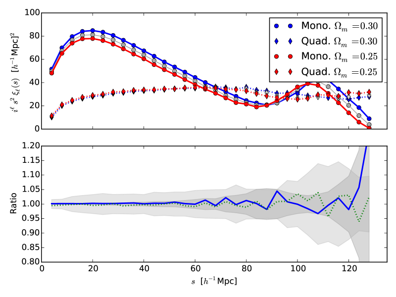
Figure 1: How the correlation function changes with distance scale. In the upper panel the lines show the average redshift-space monopole and quadrupole moments of the correlation function of halos from two N-body simulations assuming a distance redshift relation appropriate to $\Lambda$CDM with $\Omega_{m}=0.25$ (red), 0.275 (light grey) and 0.30 (blue). The distance to $z=1$ varies by 3 per cent for these cosmologies. The halos are taken from the $z=1$ outputs of two simulations with the same cosmology but different initial conditions and observed from each of the 8 corners as if along a lightcone. The halos have masses $5\times 10^{12}<M<10^{13}\,h^{-1}M_{\odot}$ and form 16 realizations of an octant of the sky cut to $0.8<z<1.2$. Note that the correlation function assuming $\Omega_{m}=0.275$ can be described to better than 10 per cent by the linear interpolation of the 0.25 and 0.30 results except where it crosses zero. The lower panel shows the ratio of the linear interpolation to the 0.275 result. The light and dark grey bands show the $1\,\sigma$ error on the mean (from the scatter of the 16 samples) of the $\Omega_{m}=0.275$ value for the quadrupole and monopole respectively. The interpolation error is below this for all scales even for such a large interpolation.

A better scheme would add at least one additional point, close to a prior guess of the maximum likelihood parameters. Adding further points in this region is desirable, with the number limited primarily by computational resources. There are three criteria which could determine where to place additional points: (1) place points where the likelihood is high, or (2) in regions where the linear interpolation performs the worst, or (3) near the edges of the parameter space (if the simplices so defined prove advantageous). The best distribution of points is likely to be dependent upon the specifics of the problem. In the presence of these additional points the interpolation begins by first finding the $n_{p}+1$ points closest to the point, $\vec{p}$, of interest whose simplex encloses $\vec{p}$. Using these $n_{p}+1$ points, find the areal coordinates, $x_{i}$ and compute $\sum_{i}x_{i}F_{i}$ as before. We note in passing that parameter redefinitions may improve the performance of any interpolation scheme and that if we have a metric on the parameter space we can define ‘near’ and ‘far’ in terms of an approximation to a prior likelihood, but we shall not pursue this route here. We also note that while we have pursued interpolation from an unstructured mesh, many of the techniques we describe below can be useful in other interpolation schemes.

3 Interpolating the data vector

Typically one treats the data vector as fixed when doing cosmological inference, but in principle it can depend upon the cosmological model if that model includes changes in the distance-redshift relation or if complex processes such as density field reconstruction are applied to the data prior to computing the power spectrum or correlation function. For the range of cosmologies usually considered the changes in the distance-redshift relation are relatively small, and smooth. A similar smoothness applies for density field reconstruction. Thus we expect any changes in our 2-point function to be smooth functions of the input parameters and hope that they can be linearly interpolated with little error.

To illustrate this point we take the positions halos from two large N-body simulations, viewed from each corner of the boxes as if they filled an octant on the sky. Sixteen samples of halos were constructed, each in a shell $0.8<z<1.2$. Holding the angular and redshift coordinates appropriate to the ‘true’ cosmology (as assumed in running the simulation) we convert to distances in three other cosmologies with different distance-redshift relations and then compute the halo auto-correlation function. For simplicity we take the distance-redshift relation to be that of $\Lambda$CDM cosmologies with $\Omega_{m}=0.25$, 0.275 and 0.3 though this is just for illustration and when analyzing data it may make more sense to use a scheme such as outlined in ref. [15]. The results are shown in figure 1 where we see that the changes are smooth functions of the input parameters and linear interpolation from the endpoints results in errors in the interior smaller than the observational error. The variation in currently allowed cosmologies is smaller than this, and thus the interpolation should perform even better when used in cosmological inference, especially if one of the places where the data are evaluated is very close to the best-fitting cosmology. For current and future surveys there is little cost to computing the correlation function or power spectrum of the data for a number of different fiducial cosmologies, so the interpolation can be made almost arbitrarily precise. For this reason we shall not investigate this in detail, and turn instead to the more complex step of interpolating the covariance matrix. This is frequently the more computationally demanding calculation and is also the least straightforward conceptually.

4 Interpolating covariance

In large-scale structure analyses it is often the case that the covariance matrix is fixed throughout the analysis, usually at a fiducial cosmology where it was determined either through analytic means or, most often, Monte Carlo simulation. Computation of the covariance matrix from Monte Carlo simulation is often the most computationally demanding step in the analysis. Using the wrong covariance matrix won’t lead to a bias on average, but it may alter the confidence levels (see e.g. ref. [16] for a recent study and see [11] for a discussion of computing parameter dependent covariance matrices in the weak lensing case). In the limit that the fluctuations are Gaussian, the dynamics given by linear perturbation theory, the tracer bias is scale independent and the 2-point functions are very well measured, the covariance matrix will be essentially fixed and all models which are close to the data will have very similar covariance matrices. Also, for sufficiently constraining data the assumption of a fixed covariance matrix is relatively good (see discussion in Appendix A). Violations of any of these assumptions (e.g. not well constrained correlation functions on large scales or at high redshift, non-linear contributions to the dynamics, violations of the scale-independent bias assumption or inclusion of the trispectrum on small scales) can lead to relevent parameter dependence of $C$ in the high likelihood regions. In this regard it is worth noting that it is reasonably straightforward to include the parameter dependence of $C$ if $C(\vec{p})$ or its inverse can be evaluated (possibly with regularization, possible simultaneously [17]) at a few locations and the parameter dependence is smooth or small. If the likelihood is insensitive to changes in $C$ with $\vec{p}$ it is even less sensitive to small interpolation errors when including that dependence. The decision on whether to invest the resources to allow interpolation of the covariance matrix will require a case-by-case analysis.

4.1 Background

Both the covariance matrix, $C$, and its inverse, the precision matrix, are symmetric, positive-definite (SPD) matrices. Given their importance in so many branches of engineering and the sciences it is no surprise that there is a vast literature on the properties of SPD matrices. The subset of SPD matrices has a rich mathematical structure, being a manifold with tangent vectors, geodesics and a metric (e.g. [18]). In particular, there are several methods for performing interpolation between such matrices at discretely sampled points in parameter space. All such interpolations implicitly depend upon a measure of distance between matrices, and there are several such distance measures. We review some of these measures, and the associated interpolations and averages, in Appendix B, and here focus on the results.

Consider linearly interpolating between an SPD matrix $M_{0}$ at $t=0$ and $M_{1}$ at $t=1$. The arithmetic interpolation is trivially $M_{t}=(1-t)M_{0}+tM_{1}$ and this is also SPD for $0\leq t\leq 1$ since the SPD matrices form a convex cone. The geometric interpolation is almost as simple, $M_{t}=M_{0}(M_{0}^{-1}M_{1})^{t}$ or the symmetric form $M_{t}=M_{0}^{1/2}(M_{0}^{-1/2}M_{1}M_{0}^{-1/2})^{t}M_{0}^{1/2}$, where the matrix power can be easily done in the diagonal basis. In fact precisely this scheme is commonly used in computer graphics to interpolate perspective changes and rotations (using quaternions in place of rotation matrices for simplicity). Unlike arithmetic interpolation, geometric interpolation gives an SPD matrix for all $t$ and so can also be used for extrapolation although we won’t make use of that feature here.

The generalization to multidimensional interpolation, as described above, is straightforward. The arithmetic mean is trivially $m^{-1}\sum_{k}M_{k}$. The geometric mean is not quite so simple, since the matrices may not all be diagonal in the same basis, however the geometric mean can be defined as the unique solution, $M$, to $\sum_{k}{\rm Log}\left(M_{k}^{-1}M\right)=0$. Interpolation then corresponds to including weights, $u_{i}$, given by the areal coordinates of the point in the simplex, i.e. solving $M=\sum_{k}u_{k}M_{k}$ or $\sum_{k}u_{k}\,{\rm Log}\left(M_{k}^{-1}M\right)=0$ (see e.g. [19] for further discussion). We discuss several techniques for solving this second equation in Appendix C.

4.2 Diagonal example

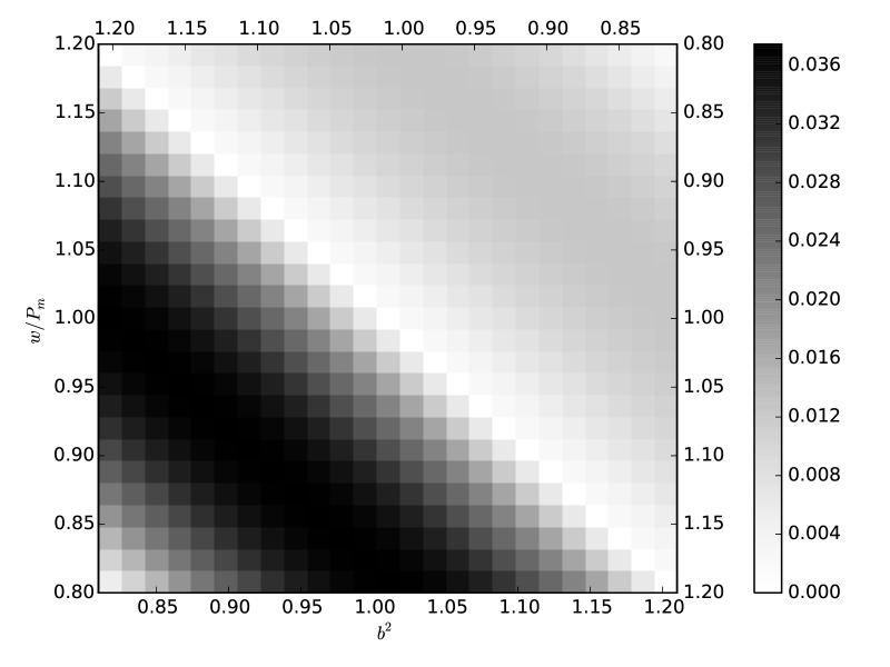
Figure 2: An example of the deviation obtained using arithmetic or geometric interpolation within a 2D simplex (i.e. a triangle) for a single element of the precision matrix corresponding to equation 4.1. The grey scale shows $\Omega_{\rm est}/\Omega_{\rm true}-1$. The lower left triangle shows the results for arithmetic interpolation, while the upper right triangle shows the results for geometric interpolation (with the upper right vertex being identified with the lower left). In both cases we interpolate the parameters linearly in $b^{2}$ and $w$. We scan the white noise level from below to above the cosmological power since the interpolations become exact in the limit that either term dominates. The dark band in the lower triangle indicates the worst-case scenario where the shot-noise and cosmological power are approximately equal.

Let us illustrate these ideas with some simple examples. In Gaussian, linear theory, if we work in $k$-space, the matrices are diagonal and all of these operations become trivial. A typical Cov in this limit is

$${\rm Cov}\left[P_{i},P_{j}\right]=\epsilon_{i}\left(P_{i}+w_{i}\right)^{2}\delta_{ij}$$ (4.1)

where $P_{i}$ is the $i$th bandpower, $\epsilon_{i}=2/N_{i}$ is a small number when the number of modes per bin, $N_{i}=V_{\rm surv}(4\pi k_{i}^{2}\Delta k)$, is large and $w_{i}=1/\bar{n}$ is the amplitude of the white- or shot-noise component. In the simplest biasing scheme, and neglecting redshift-space distortions, $P_{i}=b^{2}P_{\rm mat}(k_{i})$.

Let us consider the simplest 2D scheme where we vary just $b$ and $w$ and interpolate within the simplex $(b^{2}=b_{1}^{2},w=w_{1})$, $(b^{2}=b_{2}^{2},w=w_{1})$ and $(b^{2}=b_{1}^{2},w=w_{2})$. If we were to break equation 4.1 into its 3 parts then each could be interpolated simply, i.e. both parameters would be ‘fast’. We shall instead consider interpolating the square of the sum as a single block, treating both $b$ and $w$ as ‘slow’ parameters. In a modern survey we typically know $b$ and $w$ to order 10-20 per cent, so we will choose $\pm 20$ per cent as the range over which to vary $b^{2}$ and $\pm 20$ per cent as the range over which to vary $w$. For this situation, and for typical values of $b$ and $w$, we find that both arithmetic and geometric interpolation recover the actual result to about a per cent. The deviation is largest furthest from the vertices of the simplex, and when $b^{2}P\simeq w$, as expected. An example is shown in figure 2. We have chosen to interpolate the parameters linearly in $b^{2}$ and $w$, though we could also have chosen to interpolate in $\log b^{2}$ and $\log w$ or any mixture. The performance is not particularly dependent on this choice, but for the configuration shown linear-linear interpolation worked very well.

Although this example is somewhat artificial (we did not split the covariance matrix into its component parts and we used diagonal matrices) two characteristics can be seen. First, we see some preference for the geometric interpolation over the arithmetic one. Second, both perform quite well over the range of parameters we may expect to explore.

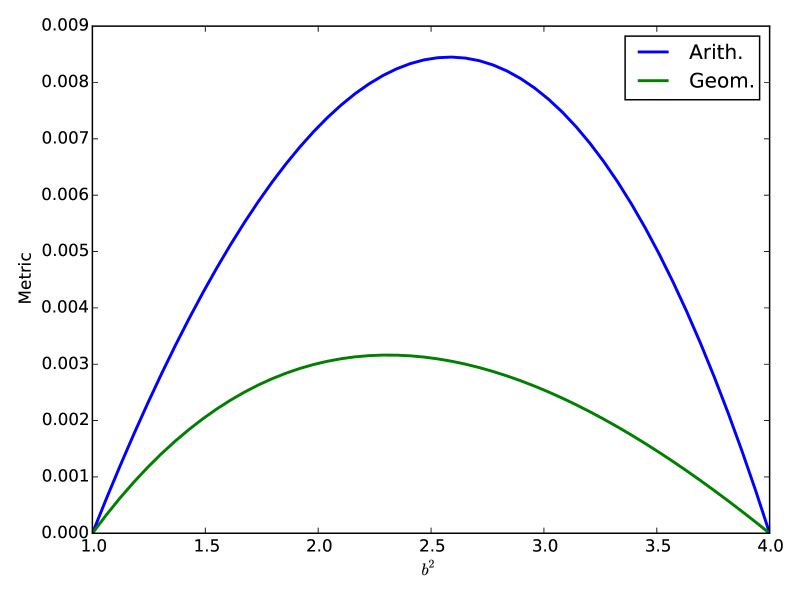
Figure 3: An example of interpolation in one dimension, in this case the large-scale bias, using arithmetic interpolation and geometric interpolation. The covariance matrix is $40\times 40$, containing entries for $\xi_{0}$ and $\xi_{2}$ evaluated at 20 points between $s=25\,h^{-1}$Mpc and $125\,h^{-1}$Mpc using linear theory with $\bar{n}=3\times 10^{-4}\,h^{3}\,{\rm Mpc}^{-3}$. The interpolated $n\times n$ precision matrix, $\Omega$, is compared to the true one using the metric $n^{-1}||C\ \Delta\Omega||_{F}$. Note the sub-percent deviation even when interpolating over such a broad range in bias at fixed shot-noise. For comparison, using a fixed covariance matrix across the range leads to an order of magnitude larger deviation by the same metric.

4.3 Matrix example

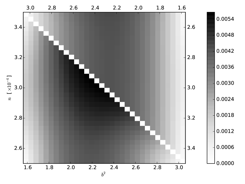
Figure 4: An example of interpolation in two dimensions (the large-scale bias and the number density). The covariance matrix is $40\times 40$, containing entries for $\xi_{0}$ and $\xi_{2}$ evaluated at 20 points between $s=25\,h^{-1}$Mpc and $125\,h^{-1}$Mpc computed using linear theory. The greyscale compares the interpolated $n\times n$ precision matrix, $\Omega$, to the true one using the metric $n^{-1}||C\ \Delta\Omega||_{F}$. The lower right half gives the results for arithmetic interpolation while the upper right gives the results for geometric interpolation (with the upper right vertex identified with the lower left). See text for further discussion.

This exercise was artificial in dealing with diagonal matrices. As a next step let us consider interpolation of non-sparse matrices. For this example we use the covariance matrix for the multipoles of the correlation function, computed in linear theory assuming Gaussian statistics and normalized by the survey volume, $V$. Motivated by the example of fitting baryon acoustic oscillations and redshift-space distortions we compute the covariance of $\xi_{\ell}(s)$ in linear theory in 20 bins of $s$ running from $25\,h^{-1}$Mpc to $125\,h^{-1}$Mpc for $\ell=0$ and $\ell=2$. This results in a $40\times 40$ covariance matrix with neighboring bins quite highly correlated.

We interpolate the full matrix (i.e. not dividing it into shot-noise and sample variance terms or pre-whitening it in any way) in $b^{2}$ holding the shot-noise fixed and compare the interpolated value to the exact calculation. The result is shown in figure 3 where we see a clear preference for geometric interpolation over arithmetic interpolation but excellent performance from both. The metric used to compare the interpolated, $n\times n$ precision matrix to that evaluated explicitly is $n^{-1}||C\,\Delta\Omega||_{F}$, where $||\cdot||_{F}$ indicates the Frobenius norm (see Appendix B). This is essentially the rms (averaged over elements) deviation from the identity of $\Omega_{\rm est}$ times $C_{\rm true}$. We see that interpolation induces sub-percent rms deviations even over such a broad range. For comparison, using a fixed covariance matrix across the range leads to an order of magnitude larger difference at the endpoints by the same metric. If we interpolate the correlation matrix (i.e. the covariance matrix normalized to unity along the diagonals) then the deviation is approximately halved, but of course we must then additionally interpolate the scaling of the diagonal entries.

Next we consider interpolating in $b^{2}$ and $\bar{n}$. In this case we interpolate over the range $1.25<b<1.75$ and $2.5\times 10^{-4}<\bar{n}<3.5\times 10^{-4}\,h^{3}{\rm Mpc}^{-3}$. The results are shown in figure 4 with the same metric as in figure 3. In this situation the preference for geometric interpolation over arithmetic interpolation is less clear, though we do find that the geometric interpolation does tend to perform better with the chosen metric. Again the absolute performance of both the arithmetic and geometric schemes is very good. If we had used a fixed covariance matrix (e.g. the one at the lower left corner) the metric at the worst point is 10 times larger than the worst-case shown in figure 4.

An alternative metric for evaluating how well we have estimated $\Omega$ is to compute tr$[C_{\rm true}\Omega_{\rm est}]-n$ where $C$ and $\Omega$ are $n\times n$ matrices. If the data are drawn from a Gaussian distribution, centered on the theory and with covariance $C_{\rm true}$, and if $\chi^{2}$ is computed using $\Omega_{\rm est}$ for the precision matrix then the average value of $\chi^{2}$ is tr$[C_{\rm true}\Omega_{\rm est}]$. For the case considered in figure 4, tr$[C_{\rm true}\Omega_{\rm est}]-n$ is never larger than about $0.03\,n$ and usually considerably less. This can be compared to the $\sqrt{2n}$ change in $\chi^{2}$ required for a $1\,\sigma$ change in the likelihood. On average, then, the error made by using the interpolated $\Omega$ in place of the ‘true’ $\Omega$ in this case is negligible compared to the statistical uncertainties in the measurement and probably small compared to the errors in determining the $C_{k}$ by Monte Carlo at each of the control points. We have investigated a number of other metrics for comparing matrices, and find a similar story by each measure.

4.4 More dimensions and simplices

As a final example we consider interpolating the covariance matrix for the multipoles of the correlation function, as above, in a 4-parameter space and over multiple simplices. We allow $b$ and $\bar{n}$ to vary, as above, but now additionally include variations in the linear growth rate, $f$, and a dilation parameter $\alpha$. The large-scale bias and shot-noise affect the amplitudes of the two contributions to the covariance, the growth rate alters the the quadrupole to monopole ratio and the dilation parameter shifts the entire correlation function in scale. Thus this parameter set allows considerable freedom in the structure of the matrices we are interpolating over.

We take the range of the parameters to be $1.25<b<1.75$, $2.5<\bar{n}<3.5\times 10^{-4}\,h^{3}\,{\rm Mpc}^{-3}$, $0.74<f<0.76$ and $0.98<\alpha<1.02$. To start, we evaluate the covariance matrices at points distributed throughout the volume (see below). Then we throw points at random within the space. For each point we find its enclosing simplex, compute the areal coordinates within that simplex and perform geometric interpolation from the 5 vertices of the simplex. Using the same metric as before, we find that the performance is excellent.

We have investigated several distributions of points, finding that they all perform quite well. First we placed the points at the vertices of a hypercube bounding the parameter set (i.e. picking either the upper or lower limits, above, for each parameter), plus an additional point at the center for a total of 17 points. The rms deviation of $C_{\rm true}\Omega_{\rm est}$ from the identity matrix for randomly thrown points was sub-percent. We also investigated using orthogonal arrays of points with 8 or 9 vertices (specifically OA(8,4,2,3) and OA(9,4,3,2) purely as illustrative examples). Within the region bounded by the points the rms deviation as again below a percent. Finally we investigated a 9 point configuration with a central point and 8 points where each parameter was individually varied to the edges of its range while the others were held fixed at the central point. Again we found that the interpolation performed very well for the enclosed points. For every case we investigated with approximately 10 points, sub-percent rms deviations were found throughout the region enclosed by the points.

Our conclusion is thus that low order interpolation from an unstructured mesh, while it may not be optimal, is very likely sufficient for upcoming surveys focused on BAO and RSD analyses of the power spectrum and correlation function. Using an interpolated precision matrix can reduce the error in the likelihood, compared to holding the precision matrix fixed, by a non-trivial factor and even a relatively coarse set of points provides an accurate interpolation. We have not considered the interesting problem of optimizing the position of the points in the mesh. Any such solution is likely to be problem specific, and to depend on the nature of the matrices being interpolated. Instead we have shown that the performance of our simple interpolation is not strongly dependent on the choice of mesh points. Finally, it is very conceivable that a more sophisticated interpolation approach could be devised and that it would save computational resources. The geometric interpolation method we have advocated has a simple generalization to techniques such a kriging, inverse distance weighting or kernel estimation. We leave such investigations to future work.

5 Conclusions

The study of large-scale structure has become a powerful means of learning about cosmology and fundamental physics. Analyses of large-scale structure data sets have become increasingly complex and sophisticated as the data themselves have grown in size and constraining power. In this paper we have focused on the comparison of theoretical models to the most common summary statistics derived from such data: the redshift-space power spectrum and correlation function. Under the assumption of a Gaussian likelihood function the computation of statistical confidence levels or goodness-of-fit of models requires knowledge of the theory, the data and the covariance matrix. In principle all three can depend on the parameters being tested though the full dependence is not usually included. We have shown that a very simple interpolation scheme from an unstructured mesh allows for an efficient way to include this parameter dependence self-consistently in the analysis at modest computational expense.

We have advocated multi-linear interpolation, under the assumption that the range of parameters being explored is relatively small and the changes smooth. For vector-valued quantities, such as the data vector of $P(k_{i})$ or $\xi_{\ell}(s_{i})$, the interpolation is straightforward. For matrix-valued quantities the best interpolation scheme is not as obvious. We have compared two, arithmetic interpolation and geometric interpolation, and found them to perform well though the geometric scheme (which uses the geometric structure of the group) can have up to half of the deviation of the simpler arithmetic scheme. As an illustrative example we showed that, for reasonable variations in shot-noise and large-scale bias, sub-percent deviations from interpolation could be achieved in predicting the linear theory covariance matrix at any point interior to the simplex. The interpolation introduces errors significantly smaller than the statistical uncertainty.

This work assumes that the data and covariance matrix have been computed at the simplex points. We leave to future work an investigation of the optimal mesh placement and efficient ways to compute the covariance matrices by conditioning the sample covariance derived from Monte Carlo simulation.

Acknowledgements: NP is supported in part by a DOE Early Career grant DE-SC0008080. MW would like to thank the Royal Observatory of Edinburgh and the Higgs Centre for their hospitality while much of this work was completed. We would like to thank Joanne Cohn and Avery Meiksin for helpful conversations on group theory and numerical methods.

Appendix A Neglecting the parameter dependence of the covariance

For large data sets, with well constrained parameters, it is often possible to neglect the parameter dependence of the covariance matrix compared to that of the mean, or theoretical prediction. This is obviously the case if the covariance matrix is independent of the parameters (e.g. the shot-noise limit for galaxy surveys) but can be true more generally. In this situation performing a simple $\chi^{2}$ analysis is enough. In this appendix we quantify how neglecting the parameter dependence of the covariance matrix affects the likelihood in some simple cases, always assuming that the ‘fixed’ covariance matrix is chosen to be close to that of the best fit model. For a discussion of how an incorrect covariance matrix affects the likelihood, see e.g. [16, 11].

As in the main text, let us assume a Gaussian form for the likelihood of the theory, $\mu$, given data, $d$, with covariance $C$:

$$-2\ln\mathcal{L}=(d-\mu)^{T}C^{-1}(d-\mu)+{\rm tr}\ln C+\cdots$$ (A.1)

then the parameter dependence can enter in the mean, $\mu(p)$, or variance, $C(p)$. Obviously we cannot make a generic statement about which is the dominant dependence, since e.g. a priori we could have $\mu$ or $C$ be $p$-independent. For the case of galaxy surveys however we can make considerable progress (see [20] for very related discussion and [21] for an investigation for the case of BAO and [22] for an investigation for the case of cosmic shear).

Let us consider how the likelihood function falls from its peak as we vary the parameters away from the best-fit point. For analytic simplicity and in order to bring out the key points we shall work in linear theory and use a $k$-space basis. Without loss of generality we can take our ‘parameters’ to be bandpowers in a $k$-bin, $p_{i}$, with the measurements of the power spectrum in the bin being $P_{i}=P(k_{i})$. With these assumptions $\mu=p_{i}$ while Cov$[P_{i},P_{j}]=\epsilon_{i}(p_{i}+w_{i})^{2}\delta_{ij}$ where $\epsilon_{i}=2/N_{i}$ is a small number when the number of independent modes per bin, $N_{i}$, is large and we have written the white- or shot-noise component as $w_{i}$. Our covariance matrix is most parameter dependent when $w_{i}\equiv 0$, or we are in the ‘sample variance limit’. We shall therefore make this assumption. Note that the covariance is diagonal in $k$-space in linear theory, so the log-likelihood becomes

$$-2\ln\mathcal{L}=\sum_{i}\ln|C_{ii}|+\frac{(P_{i}-p_{i})^{2}}{C_{ii}}+\cdots=\sum_{i}\ln p_{i}^{2}+\frac{(P_{i}-p_{i})^{2}}{\epsilon_{i}p_{i}^{2}}+\cdots$$ (A.2)

where $\cdots$ represents terms independent of $p_{i}$. Note how the first term (from the variation of the covariance matrix) is independent of $\epsilon_{i}$ while the second becomes increasingly more important as $\epsilon_{i}\to 0$. For large amounts of data, small $\epsilon_{i}$, the parameter dependence of the covariance term only becomes important once we are far from the peak of the likelihood function, i.e. for models which are disfavored by the data. To see this, note that for a model to be allowed $p_{i}$ must be close to $P_{i}$, i.e. within $\sqrt{\epsilon}$. For such variations, we can compute the difference between allowing the covariance to vary and holding it fixed at the peak of the likelihood. This difference scales as $\sqrt{\epsilon}$. The parameter dependence of the covariance therefore only becomes important for models disfavored by the data.

An alternative approach [20] is to look at the Fisher matrix, i.e. the expectation value of the Hessian of the log-likelihood. For a Gaussian this becomes

$$F_{\alpha\beta}\propto{\rm tr}\left[C^{-1}C_{,\alpha}C^{-1}C_{,\beta}\right]+\mu_{,\alpha}C^{-1}\mu_{,\beta}$$ (A.3)

where $,\alpha$ denotes a derivative with respect to parameter $p_{\alpha}$ and we have chosen Greek indices to label the parameters which can now be arbitrary. The Fisher matrix represents the curvature of the likelihood around the peak, assuming ‘typical’ data. Once again, note that the first term (arising from the parameter-dependence of the covariance) is independent of the overall normalization of $C$ while the second term scales as the inverse of the normalization. It is easy to show that for bandpowers as parameters and the same assumptions as above the first term is $\mathcal{O}(\sum_{i}p_{i}^{-2})$ while the second is $N_{i}$ times larger and so dominates in the large-volume, high-precision limit.

Appendix B Distance measures for SPD matrices

In this appendix we quickly review some common distance measures on the space of symmetric, positive-definite (SPD) matrices.

The most basic distance measure is the Frobenius norm (sometimes called the Hilbert-Schmidt norm). The Frobenius norm is the one induced by the inner product on matrices thought of as a vector space: $\langle\mathbf{A},\mathbf{B}\rangle={\rm tr}(\mathbf{AB}^{T})$. If we work with symmetric matrices, $||\mathbf{A}||=\sqrt{{\rm tr}(\mathbf{A}^{2})}$.

We can also use the Kullback-Liebler divergence (or information gain). The KL divergence between two zero-mean Gaussians with covariances $C_{a}$ and $C_{b}$ is

$$D_{KL}(C_{a}||C_{b})=\frac{1}{2}\left[{\rm tr}\left(C_{a}C_{b}^{-1}\right)-\log\det\left(C_{a}C_{b}^{-1}\right)-N\right]$$ (B.1)

with $C_{a}$ and $C_{b}$ $N\times N$ matrices and $D\geq 0$ with equality only if $C_{a}=C_{b}$. A distance measure can be constructed from $D_{KL}$ by symmetrizing the arguments. If $\lambda_{i}$ are the eigenvalues of $C_{a}^{-1}C_{b}$ then

$$D_{KL}^{\rm sym}(C_{a},C_{b})=\frac{1}{2}\sum_{i=1}^{N}\left(\sqrt{\lambda_{i}}-\frac{1}{\sqrt{\lambda_{i}}}\right)^{2}$$ (B.2)

and the square root of $D_{KL}^{\rm sym}$ is a distance measure which is invariant under congruent transformations and inversion.

Finally we can consider the space of positive-definite symmetric matrices as a manifold, with a Riemannian metric defined by the Frobenius dot product on the tangent space at any point. The geodesic distance between matrices $C_{a}$ and $C_{b}$ then becomes [e.g. 19]

$$D_{R}(C_{a},C_{b})=||{\rm Log}(C_{a}^{-1}C_{b})||_{F}=\sqrt{\sum_{i=1}^{N}\log^{2}\lambda_{i}}$$ (B.3)

where the $\lambda_{i}$ in the last equality are the eigenvalues of the matrix $C_{a}^{-1}C_{b}$. Note that for any positive-definite symmetric matrix $M$ we can decompose it into a diagonal and orthogonal matrix as $M=UDU^{T}$ with $D$ containing the eigenvalues and $U$ the eigenvectors of $M$. In this basis taking Log$M$ simply becomes taking the log of the diagonal entries, i.e. ${\rm Log}M=U\ln(D)U^{T}$.

Each of these different distance measures naturally lead to a different interpolation scheme. Consider for example taking the ‘average’. Under the Frobenius norm the arithmetic average, $\bar{C}$, of the matrices $C_{k}$ minimizes the squared distance: $\sum_{k}\left|\bar{C}-C_{k}\right|^{2}$. The geodesic distance leads to geometric means of matrices as the appropriate average, while the KL-based distance gives the geometric mean of the arithmetic and harmonic means [24]. Similar situations arise when performing interpolation, as described in the main text.

Appendix C Solving the geometric interpolation equation

Suppose we are given the values of the covariance matrix at the $m=n_{p}+1$ corners of a simplex, $C_{k}$, and the areal coordinates $u_{k}$ corresponding to the (interior) point for which we want the interpolated value of the precision matrix, $\Omega$. In order to interpolate geometrically we need to find the matrix $\Omega$ which solves

$$G(\Omega)\equiv\sum_{k=1}^{m}u_{k}{\rm Log}\left(C_{k}\Omega\right)=0\quad.$$ (C.1)

One method would be to use Newton’s algorithm for matrix valued functions of matrices. This requires the (Fréchet) derivative of $G$. Fast numerical algorithms for computing both the logarithm and its derivative exist [25], but are complex. A more standard approach is to use a variant of Broyden’s method [26], or other quasi-Newton methods, which do not require the explicit evaluation of a derivative. By stacking the columns of our matrices atop each other we can turn $n\times n$ matrices into $n^{2}$-dimensional vectors (this is the “vec” operation, equivalent to replacing pairs of indices, $ij$, by a super-index, $I$) and the problem reduces to a standard one of simultaneously solving multiple non-linear equations. Various efficient and general algorithms for this problem exist, however convergence can be difficult to achieve when the number of terms in the sum and the dimension of the matrices becomes large.

The method we have used is a fixed point algorithm due to ref. [24]. If we rotate our bases by $\Omega_{1}^{-1/2}$ to set $\Omega_{1}=1$ and left and right multiply by $\Omega^{1/2}$ and $\Omega^{-1/2}$ we can write equation C.1 as

$${\rm Log}\hat{\Omega}=-\sum_{k=2}^{m}u_{k}^{\prime}\ {\rm Log}\left(\hat{\Omega}^{1/2}\hat{C}_{k}\hat{\Omega}^{1/2}\right)$$ (C.2)

where hats denote the matrices in rotated coordinates and the $u_{k}^{\prime}$ are $u_{k}$ divided by $1-\sum_{k=2}^{m}u_{k}$. Ref. [24] shows that this can be solved for $S={\rm Log}\hat{\Omega}$ using a fixed point iteration

$$S^{\ell+1}=\alpha S^{\ell}+(\alpha-1)\sum_{k=2}^{m}u_{k}^{\prime}\ {\rm Log}\left(\exp(S^{\ell}/2)\hat{C}_{k}\exp(S^{\ell}/2)\right)$$ (C.3)

starting at $S^{0}=\sum_{k}u_{k}^{\prime}\ {\rm Log}\hat{\Omega}_{k}$. This converges for $\alpha=(m+a)/(m+a+1)$ for any integer $a>0$ and we have found that convergence is typically very rapid. In fact for the situations we have explored the starting guess is already a good approximation to the geometric mean. When checking for convergence it is easier to use the symmetric form

$$\Omega^{1/2}G(\Omega)\Omega^{-1/2}=0=\sum_{k=1}^{m}u_{k}{\rm Log}\left(\Omega^{1/2}C_{k}\Omega^{1/2}\right)$$ (C.4)

for which the arguments of the Log are explicitly SPD, which allows for quick computation.

References

- [1] W. R. Gilks, S. Richardson, and D. J. Spiegelhalter, Markov Chain Monte Carlo in Practice. Chapman and Hall, London, 1996 (ISBN: 0-412-05551-1).
- [2] W. R. Gilks, Markov Chain Monte Carlo In Practice. Chapman and Hall/CRC, 1999.
- [3] P. Mukherjee, D. Parkinson, and A. R. Liddle, A Nested Sampling Algorithm for Cosmological Model Selection, ApJL 638 (Feb., 2006) L51–L54, [astro-ph/0508461].
- [4] X. Xu, M. White, N. Padmanabhan, D. J. Eisenstein, J. Eckel, K. Mehta, M. Metchnik, P. Pinto, and H.-J. Seo, A New Statistic for Analyzing Baryon Acoustic Oscillations, ApJ 718 (Aug., 2010) 1224–1234, [arXiv:1001.2324].
- [5] D. J. Eisenstein, H.-J. Seo, E. Sirko, and D. N. Spergel, Improving Cosmological Distance Measurements by Reconstruction of the Baryon Acoustic Peak, ApJ 664 (Aug., 2007) 675–679, [astro-ph/0604362].
- [6] C. Blake, S. Brough, M. Colless, C. Contreras, W. Couch, S. Croom, T. Davis, M. J. Drinkwater, K. Forster, D. Gilbank, M. Gladders, K. Glazebrook, B. Jelliffe, R. J. Jurek, I.-H. Li, B. Madore, D. C. Martin, K. Pimbblet, G. B. Poole, M. Pracy, R. Sharp, E. Wisnioski, D. Woods, T. K. Wyder, and H. K. C. Yee, The WiggleZ Dark Energy Survey: the growth rate of cosmic structure since redshift , MNRAS 415 (Aug., 2011) 2876–2891, [arXiv:1104.2948].
- [7] C. Blake, S. Brough, M. Colless, C. Contreras, W. Couch, S. Croom, D. Croton, T. M. Davis, M. J. Drinkwater, K. Forster, D. Gilbank, M. Gladders, K. Glazebrook, B. Jelliffe, R. J. Jurek, I.-h. Li, B. Madore, D. C. Martin, K. Pimbblet, G. B. Poole, M. Pracy, R. Sharp, E. Wisnioski, D. Woods, T. K. Wyder, and H. K. C. Yee, The WiggleZ Dark Energy Survey: joint measurements of the expansion and growth history at , MNRAS 425 (Sept., 2012) 405–414, [arXiv:1204.3674].
- [8] L. Anderson, É. Aubourg, S. Bailey, F. Beutler, V. Bhardwaj, M. Blanton, A. S. Bolton, J. Brinkmann, J. R. Brownstein, A. Burden, C.-H. Chuang, A. J. Cuesta, K. S. Dawson, D. J. Eisenstein, S. Escoffier, J. E. Gunn, H. Guo, S. Ho, K. Honscheid, C. Howlett, D. Kirkby, R. H. Lupton, M. Manera, C. Maraston, C. K. McBride, O. Mena, F. Montesano, R. C. Nichol, S. E. Nuza, M. D. Olmstead, N. Padmanabhan, N. Palanque-Delabrouille, J. Parejko, W. J. Percival, P. Petitjean, F. Prada, A. M. Price-Whelan, B. Reid, N. A. Roe, A. J. Ross, N. P. Ross, C. G. Sabiu, S. Saito, L. Samushia, A. G. Sánchez, D. J. Schlegel, D. P. Schneider, C. G. Scoccola, H.-J. Seo, R. A. Skibba, M. A. Strauss, M. E. C. Swanson, D. Thomas, J. L. Tinker, R. Tojeiro, M. V. Magaña, L. Verde, D. A. Wake, B. A. Weaver, D. H. Weinberg, M. White, X. Xu, C. Yèche, I. Zehavi, and G.-B. Zhao, The clustering of galaxies in the SDSS-III Baryon Oscillation Spectroscopic Survey: baryon acoustic oscillations in the Data Releases 10 and 11 Galaxy samples, MNRAS 441 (June, 2014) 24–62, [arXiv:1312.4877].
- [9] M. White, B. Reid, C.-H. Chuang, J. L. Tinker, C. K. McBride, F. Prada, and L. Samushia, Tests of redshift-space distortions models in configuration space for the analysis of the BOSS final data release, MNRAS 447 (Feb., 2015) 234–245, [arXiv:1408.5435].
- [10] M. White, Reconstruction within the Zeldovich approximation, MNRAS 450 (July, 2015) 3822–3828, [arXiv:1504.0367].
- [11] C. B. Morrison and M. D. Schneider, On estimating cosmology-dependent covariance matrices, JCAP 11 (Nov., 2013) 9, [arXiv:1304.7789].
- [12] K. Heitmann, D. Higdon, M. White, S. Habib, B. J. Williams, E. Lawrence, and C. Wagner, The Coyote Universe. II. Cosmological Models and Precision Emulation of the Nonlinear Matter Power Spectrum, ApJ 705 (Nov., 2009) 156–174, [arXiv:0902.0429].
- [13] H. Coxeter, Introduction to geometry. Wiley classics library. Wiley, 1969.
- [14] V. T. Rajan, Optimality of the delaunay triangulation in rd, in Proceedings of the Seventh Annual Symposium on Computational Geometry, SCG ’91, (New York, NY, USA), pp. 357–363, ACM, 1991.
- [15] F. Zhu, N. Padmanabhan, and M. White, Optimal redshift weighting for baryon acoustic oscillations, MNRAS 451 (July, 2015) 4755–4762, [arXiv:1411.1424].
- [16] A. Taylor, B. Joachimi, and T. Kitching, Putting the precision in precision cosmology: How accurate should your data covariance matrix be?, MNRAS 432 (July, 2013) 1928–1946, [arXiv:1212.4359].
- [17] M. Pourahmadi, M. J. Daniels, and T. Park, Simultaneous modelling of the cholesky decomposition of several covariance matrices, Journal of Multivariate Analysis 98 (2007), no. 3 568 – 587.
- [18] S. Helgason, Differential geometry, Lie groups, and symmetric spaces, vol. 80. Academic press, 1979.
- [19] M. Moakher and P. Batchelor, Symmetric Positive-Definite Matrices: From Geometry to Applications and Visualization. Mathematics and Visualization. Springer Berlin Heidelberg, 2006.
- [20] M. Tegmark, Measuring Cosmological Parameters with Galaxy Surveys, Physical Review Letters 79 (Nov., 1997) 3806–3809, [astro-ph/9706198].
- [21] A. Labatie, J. L. Starck, and M. Lachièze-Rey, Effect of Model-dependent Covariance Matrix for Studying Baryon Acoustic Oscillations, ApJ 760 (Dec., 2012) 97, [arXiv:1210.0878].
- [22] T. Eifler, P. Schneider, and J. Hartlap, Dependence of cosmic shear covariances on cosmology. Impact on parameter estimation, A&A 502 (Aug., 2009) 721–731, [arXiv:0810.4254].
- [23] S. T. Smith, Covariance, subspace, and intrinsic crame r-rao bounds, Signal Processing, IEEE Transactions on 53 (2005), no. 5 1610–1630.
- [24] M. Moakher, On the averaging of symmetric positive-definite tensors, Journal of Elasticity 82 (2006), no. 3 273–296.
- [25] A. H. Al-Mohy, N. J. Higham, and S. D. Relton, Computing the Fréchet derivative of the matrix logarithm and estimating the condition number, j-SISC 35 (2013), no. 4 C394–C410.
- [26] C. G. Broyden, A new method of solving nonlinear simultaneous equations, j-COMP-J 12 (Feb., 1969) 94–99.