Improved Algorithms for Radar-Based Reconstruction of Asteroid Shapes

Abstract

We describe our implementation of a global-parameter optimizer and Square Root Information Filter (SRIF) into the asteroid-modelling software shape. We compare the performance of our new optimizer with that of the existing sequential optimizer when operating on various forms of simulated data and actual asteroid radar data. In all cases, the new implementation performs substantially better than its predecessor: it converges faster, produces shape models that are more accurate, and solves for spin axis orientations more reliably. We discuss potential future changes to improve shape’s fitting speed and accuracy.

I. Introduction

Earth-based radar is a powerful tool for gathering information about bodies in the Solar System. Radar observations can dramatically improve the determination of the physical properties and orbital elements of small bodies (such as asteroids and comets). An important development in the past two decades has been the formulation and implementation of algorithms for asteroid shape reconstruction based on radar data (Hudson, 1993; Hudson & Ostro, 1994; Ostro et al., 1995; Hudson & Ostro, 1995). This problem is not trivial because it requires the joint estimation of the spin state and shape of the asteroid. Because of the nature of radar data, recovery of the spin state depends on knowledge of the shape and vice versa. Even with perfect spin state information, certain peculiarities of radar images (such as the two-to-one or several-to-one mapping between surface elements on the object and pixels within the radar image) make recovery of the physical shape challenging (Ostro, 1993). This is a computationally intensive problem, potentially involving hundreds to thousands of free parameters and millions of data points.

Despite the computational cost, astronomers are keen on deriving shape and spin information from asteroid radar images. The most compelling reason to do so is the fact that radar is the only Earth-based technique that can produce detailed three-dimensional information of near-Earth objects. This is possible because radar instruments achieve spatial resolutions that dramatically surpass the diffraction limit. In other words, radar instruments can resolve objects substantially smaller than the beamwidth of the antenna used to obtain the images. For example, the Arecibo telescope, the primary instrument used for the data presented in this paper, has a beamwidth of ${\sim}2$ arcminutes at the nominal 2380 MHz frequency of the radar. Yet observers can easily gather shape information to an accuracy of decameters for objects several millions of kilometers from Earth, achieving an effective spatial resolution of ${\sim}1$ milliarcsecond.

Radar has other advantages as well. Unlike most observational techniques inside the Solar System, radar does not rely on any external sources of light, be it reflected sunlight, transmitted starlight, or thermal emission. This human-controlled illumination allows for greater flexibility with respect to the observations. In addition, because of the wavelengths involved, radar observations can be performed during the day, further enhancing this flexibility. Radar also has the ability to probe an object’s sub-surface properties, which can give important information about the object such as porosity, surface and sub-surface dielectric constant, and the presence of near-surface ice.

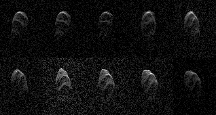
Figure 1.— A time-series of range-Doppler images of the asteroid 2000 ET70 (Naidu et al., 2013), starting in the top left and proceeding to the right. The epochs of consecutive images are separated by 18 minutes. Distance from the observer increases downwards, and Doppler increases to the right.

Asteroid shape data are important for various reasons. For certain asteroids, reliable determination of an orbital future cannot be determined without shape and spin information. The Yarkovsky effect, for example, can change an asteroid’s semi-major axis at a rate of ${\sim}10^{-4}$ AU/My for km-sized objects (Vokrouhlický et al., 2000; Bottke et al., 2006; Nugent et al., 2012). This effect occurs because the rotating body absorbs sunlight and then re-emits that light in a non-sunward direction, resulting in a gentle perturbation to the asteroid’s orbit. The Yarkovsky effect is greatly dependent on the shape of the object, since re-emission of absorbed sunlight is a surface phenomenon. It is responsible for the largest source of uncertainty in trajectory predictions for near-Earth asteroids (NEAs) with sizes under 2 km, and it must be taken into account when evaluating impact probabilities (Giorgini et al., 2002; Chesley et al., 2014; Farnocchia et al., 2013).

Knowledge of the shape also provides clues about the formation and interaction history of asteroids. For example, radar-derived shapes of asteroids have been instrumental in identifying binary asteroids and contact binaries, which represent ${\sim}16\%$ and ${\sim}10\%$ of the population, respectively (Margot et al., 2002; Benner et al., 2008). They have also provided strong evidence that NEA binaries form by a spin-up and mass shedding process (Margot et al., 2002; Ostro et al., 2006). For single asteroids, knowledge of the morphology guides interpretation of the collisional history and surface modification processes.

Shapes also affect spin evolution during two-body interactions (e.g., torques during close planetary encounters) and orbital evolution of binary NEAs (e.g., tidal, gravitational, and non-gravitational interactions between components) (e.g., Margot et al., 2002; Ostro et al., 2006; Scheeres et al., 2006; Ćuk & Nesvorný, 2010; Jacobson et al., 2014; Naidu & Margot, 2015). Finally, shapes are needed when calculating the gravity environment near asteroids, which is of special importance for proximity operations (Fujiwara et al., 2006; Naidu et al., 2013; Nolan et al., 2013; Takahashi & Scheeres, 2014).

The determination of an asteroid’s spin state from radar data is equally valuable. In contrast to lightcurve period determinations, which are neither sidereal nor synodic, the radar-based measurements yield sidereal periods. These estimates are needed to test the agreement between physical theories and observations, e.g., the change in asteroid spin rate due to sunlight (e.g., Taylor et al., 2007; Lowry et al., 2007) and subsequent shape evolution (e.g., Harris et al., 2009; Fahnestock & Scheeres, 2009). Proper modeling of the Yarkovsky perturbations to an asteroid’s heliocentric orbit or to the evolution of binary orbits (e.g., Margot et al., 2015) also require knowledge of the spin state. Finally, important insights can be gained about asteroid physical properties and collisional evolution from the spin distributions of both regular rotators and non-principal-axis rotators (e.g., Pravec et al., 2002).

II. Current Method

Asteroid shapes and spin states are currently modeled using the shape software package (Hudson, 1993; Magri et al., 2007). shape takes a model for the asteroid, which is based on both shape and spin parameters, as well as scattering behavior, and projects that model into the same space as that of the radar observables. This space, called the range-Doppler space, has dimensions of range and line-of-sight velocity (figure 1). shape can also handle optical lightcurve data when fitting for asteroid shapes, but we did not use this capability in this paper.

shape then compares the mapping of the model into this space to the radar observables, and makes changes to the model parameters in an attempt to minimize the sum of squares of residuals. shape uses increasing model complexity to build up a representation for the asteroid, from a basic ellipsoid model to capture gross features, to a spherical harmonic model which can represent finer surface elements (See section V.1) and finally a model based on contiguous triangular facets (hereafter vertex model). The spin state is generally estimated in the early stages of the shape fitting – this is normally done by using trial values of the spin state while simultaneously fitting for the shape itself.

shape currently uses a Sequential Parameter Fit (SPF) mechanism to adjust the model following a comparison between the model projection and the radar observables. SPF minimizes $\chi^{2}$ using a “bracket and Brent” method (Press et al., 1992) – for each iteration, this process minimizes $\chi^{2}$ for variations in that individual parameter only, while all other parameters are held constant. This process is not only slow, but it also does not guarantee convergence on a global minimum, or even the nearest local minimum, because minimization always progresses along a single parameter axis at a time. We have worked towards replacing the SPF currently implemented in shape with a modified Square Root Information Filter (SRIF), as outlined in section III.1.

III. Solution via Normal Equations

Before detailing the mechanics of the SRIF, it is worth discussing the Normal Equations Method (NEM), to which SRIF is related  (Press et al., 1992). A classical NEM minimizes the weighted residuals between a model and data with noise assumed to be Gaussian by determining the direction in parameter space in which $\chi^{2}$ is decreasing fastest. Specifically, suppose one has a set of $m$ observables, $\vec{z}$, with weights that are the diagonal elements of an $m\times m$ matrix $W$, and a model function $\vec{f}(\vec{x})$, where $\vec{x}$ is an $n$-dimensional parameter vector. Assuming independent data points with Gaussian-distributed errors, the probability of the model matching the data is given by

$$p(\vec{f}(\vec{x})\ |\ \vec{z})\propto p(\vec{z}\ |\ \vec{f}(\vec{x}))\propto\exp(-\frac{1}{2}\vec{R}^{\intercal}W\vec{R}),$$

where $\vec{R}=\vec{z}-\vec{f}(\vec{x})$. Therefore maximizing the model probability is the same as minimizing the value

$$\chi^{2}(\vec{x})=\vec{R}^{\intercal}W\vec{R}.$$

Perturbing $\vec{x}$ by some amount, $\vec{\delta x}$, and minimizing $\chi^{2}(\vec{x})$ over $\vec{\delta x}$ yields

$$(A^{\intercal}WA)\vec{\delta x}=A^{\intercal}W\vec{R},$$

where

$$A=\frac{\partial\vec{R}}{\partial\vec{x}}.$$

Thus, changing one’s parameter vector by

$$\vec{\delta x}=(A^{\intercal}WA)^{-1}A^{\intercal}W\vec{R}$$ (1)

yields a decrease in $\chi^{2}(\vec{x})$. For non-linear systems, this process is repeated multiple times until the change in $\chi^{2}$ from one iteration to the next has passed below a fiducial fraction. Equation 1 is also known as the weighted normal equation.

A major issue with NEM is the computation of the inverse of the matrix $A^{\intercal}WA$. This matrix has $n^{2}$ elements and thus can be quite large for a model with many parameters. In addition, numerical stability can be a serious issue – $A^{\intercal}WA$ may be ill-conditioned, and thus taking the inverse can result in numerical errors (see Appendix).

One way to quantify the issue of numerical stability is by using the condition number $\kappa(M)$, where $\kappa(M)\equiv||M||*||M^{-1}||$. A smaller $\kappa(M)$ corresponds to a better conditioned matrix $M$, meaning that fewer errors will accrue in the calculation of $M^{-1}$.

Since

$$\kappa(A^{\intercal}WA)\propto\kappa(A)^{2}$$

and

$$\kappa(A)>1$$

for non-orthogonal matrix A, the classical NEM increases the risk of numerical instabilities

Finally, for problems involving a very large number of observations and model parameters, even the calculation of $(A^{\intercal}WA)$ is non-trivial, as this matrix multiplication scales like $m^{2}n$. The number of observations needed for an asteroid shape reconstruction typically number in the millions, with potentially $10^{2}-10^{5}$ free parameters.

III.1. Square Root Information Filter

The Square Root Information Filter (SRIF) was originally developed by Bierman in 1977 (Bierman, G. J. (1977), Lawson & Hanson (1995)). The algorithm minimizes $\chi^{2}$ for time series data with Gaussian errors, and is inspired by the Kalman filter algorithm. SRIF is more stable, more accurate, and faster than the algorithm currently used in shape. SRIF is also more numerically stable (and, in some cases faster) than a solution via normal equations. Our implementation of SRIF includes some changes to the original algorithm, which will be discussed in section IV.

SRIF gets around all the problems described above by utilizing matrix square roots and Householder operations (see Bierman, G. J. (1977), pg. 59) to increase the numerical stability when determining $\delta\vec{x}$. Instead of minimizing $\chi^{2}$, SRIF minimizes

$$Q=(\chi^{2})^{\frac{1}{2}}=||W^{\frac{1}{2}}\vec{R}||,$$

where $W^{\frac{1}{2}}$ is the square root of the matrix $W$, defined such that

$$W=W^{\frac{1}{2}}W^{\frac{1}{2}}.$$

In general, the square root of a matrix is multivalued, however since $W$ is positive-semidefinite, all square roots are real. We select the positive root by convention.

Then, along similar lines as NEM, a change of $\vec{\delta x}$ is introduced to the parameter vector $\vec{x}$, and $Q^{\prime}=Q(\vec{x}+\vec{\delta x})$ is minimized over this change.

$Q^{\prime}$ is smallest when

$$||W^{\frac{1}{2}}\vec{R}(\vec{x}+\vec{\delta x})||\approx||W^{\frac{1}{2}}(\vec{R}(\vec{x})+A\vec{\delta x})||$$

$$=||W^{\frac{1}{2}}\vec{R}(\vec{x})+W^{\frac{1}{2}}A\vec{\delta x}||$$

is minimized.

A matrix $H$ is defined such that $HW^{\frac{1}{2}}A$ is upper triangular. $H$ is orthogonal and can be generated by the product of $n$ Householder operation matrices. Note that the orthogonality of $H$ guarantees that

$$||W^{\frac{1}{2}}\vec{R}(\vec{x})+W^{\frac{1}{2}}A\vec{\delta x}||=||H(W^{\frac{1}{2}}\vec{R}(\vec{x})+W^{\frac{1}{2}}A\vec{\delta x})||$$

$$=||HW^{\frac{1}{2}}\vec{R}(\vec{x})+HW^{\frac{1}{2}}A\vec{\delta x}||.$$

From the definition of $H$, $HW^{\frac{1}{2}}A$ can be rewritten as

$$HW^{\frac{1}{2}}A=\left(\begin{array}[]{c}A^{\prime}\\ Z\end{array}\right),$$

where $A^{\prime}$ is an $n\times n$ upper-triangular matrix, and $Z$ is the $(m-n)\times n$ zero-matrix. Then, rewriting

$$HW^{\frac{1}{2}}\vec{R}(\vec{x})=\left(\begin{array}[]{c}\vec{R_{x}^{\prime}}\\ \vec{R_{z}^{\prime}}\end{array}\right),$$

where $R_{x}^{\prime}$ and $R_{z}^{\prime}$ are $m\times 1$ and $(n-m)\times 1$ arrays, respectively, yields

$$Q^{\prime}=\left|\left|\left(\begin{array}[]{c}\vec{R_{x}^{\prime}}+A^{\prime}\vec{\delta x}\\ \vec{R_{z}^{\prime}}+Z\vec{\delta x}\end{array}\right)\right|\right|=\left|\left|\left(\begin{array}[]{c}\vec{R_{x}^{\prime}}+A^{\prime}\vec{\delta x}\\ \vec{R_{z}^{\prime}}\end{array}\right)\right|\right|.$$

This is clearly minimized over $\delta x$ when

$$\vec{R_{x}^{\prime}}=-A^{\prime}\vec{\delta x}$$

or

$$\vec{\delta x}=-A^{\prime-1}\vec{R_{x}^{\prime}}.$$ (2)

Since $A^{\prime}$ is upper triangular, its inverse can be easily calculated, and singularity can be trivially detected. Furthermore, the condition number of the inverted matrix is proportional to $\kappa(A)$, as opposed to $\kappa(A)^{2}$ in the NEM case.

Finally, note that $A^{\intercal}WA$ is never calculated, which, as mentioned in section III, is a computationally intensive calculation.

IV. Additions to SRIF

IV.1. Optimizations

The number of operations necessary to generate the Householder matrix $H$ grows as O($n^{2}(m-n)$), where the number of observations $m$ always exceeds the number of parameters $n$. Although this growth profile is favorable with respect to $m$ when compared to that of NEM (O($m^{2}n$)), it becomes problematic for high resolution models (large $n$). To maintain good performance in large $n$ situations, we have implemented three main optimizations to the standard SRIF.

Our first addition is to run the matrix triangularization simultaneously on multiple cores, which results in a significant speed-up. Note that although Householder matrices are generated iteratively, any given iteration $k$ requires $n-k$ column-wise operations, and each of these operations are independent from each-other. Therefore, the Householder matrix calculations can be done in a thread-safe manner.

The second addition we made to the standard SRIF is the inclusion of a secondary $\chi^{2}$ minimization for the scaling of $\vec{\delta{x}}$, so that

$$Q^{\prime}=Q(\vec{x}+\alpha\vec{\delta x})$$

is minimized over $\alpha$. This minimization is done with an eleven point grid search for $\alpha$, from $\alpha=10^{-3}$ to $\alpha=10^{3.5}$. The additional minimization adds a trivial additional computation cost to the overall minimization of $\chi^{2}$, but allows for faster convergence, and the possibility of skipping over local minima in the $\chi^{2}$-space.

The final change we made to the underlying SRIF algorithm also granted the largest speed improvement. Even with the optimizations described above, the O$(n^{2}(m-n))$ nature of the triangularization algorithm scales the computational cost drastically with increased model complexity. Furthermore, the need to store a derivative matrix for each iteration results in sizeable memory overhead when working with large datasets. To mitigate this problem, we modified the SRIF algorithm to select a subset of the nominal free parameters during each parameter vector adjustment, and to only fit for that subset. We tried a variety of subset selection methods, and concluded after testing that a “semi-random” mode was the most effective. During each parameter vector adjustment, this mode randomly selects a fixed number, $b$, of parameters from the nominal set of parameters $\{x_{s}\}$ for which the condition

$$k_{s}\leq\lfloor{i*\frac{b}{n}}\rfloor$$

is satisfied, where $k_{s}$ is the total number of times parameter $x_{s}$ has been considered over the course of the entire fit, $i$ is the total number of times that the parameter vector has been adjusted, $n$ is the total number of nominal free parameters, and $\lfloor\ \rfloor$ is the round down operator.

When fitting for both shape and spin state simultaneously (Section V.3), the spin axis orientation parameters were always included in the fit at each parameter vector adjustment step.

IV.2. Penalty functions

The SPF routine can currently fit models to data while taking into account a suite of “penalty functions” that favor models with desirable properties. In a way, these penalty functions serve to make the fit operate in a more global context – there may be a local minimum in $\chi^{2}$-space towards which the fitting algorithm would want to tend, but that minimum can be ruled out a priori thanks to physical considerations. These penalty functions include limits on ellipsoid axis ratios to avoid absurdly elongated or flattened shapes, constraints on shape concavities to avoid unrealistic surface topographies, and limits on the model center of mass distance from the image center, to name a few. We have implemented these penalty functions in the SRIF framework by redefining the residual vector as

$$\vec{R}^{\prime\prime}=\left(\begin{array}[]{c}\vec{z}-\vec{f}(\vec{x})\\ \vec{p_{w}}\end{array}\right),$$

where

$$\vec{p_{w}}=\left(\begin{array}[]{c}p_{1}\times w_{1}\\ \vdots\\ p_{N}\times w_{N}\end{array}\right)$$

for which $\{p_{i}\}$ , $\{w_{i}\}$ are the set of penalty functions and penalty weights, respectively, and

$$A^{\prime\prime}=\frac{\partial\vec{R^{\prime\prime}}}{\partial\vec{x}}.$$

The algorithm then progresses as described in section III.1, with $\vec{R}^{\prime\prime}$ replacing $\vec{R}$ and $A^{\prime\prime}$ replacing $A^{\prime}$.

V. Results

We tested our implementation with three different types of data. First, we generated simple spherical harmonic shapes and simulated images with Gaussian noise. Second, we used existing shape models of asteroids and simulated images with $\chi^{2}$-distributed errors, the appropriate model for radar noise. Third, we used an actual asteroid radar data set. In all cases, we fit the images to recover the shapes using SRIF, SPF, and a third-party Levenberg-Marquardt algorithm (LM), a standard optimizing algorithm which is used across a wide variety of fields and applications (Press et al., 1992). Except where otherwise noted, our tests did not involve adjustments to parameters controlling the radar scattering law, ephemeris corrections, or spin axis orientation.

V.1. Simulated data with artificial shapes

These tests consisted of generating an initial basic shape (either spherical, oblate ellipsoid, or prolate ellipsoid), and randomly perturbing the spherical harmonic representation of this shape to get a new, non-trivial object.

Simulated range-Doppler images of this object were generated, and these images were fit for using the three aforementioned algorithms. This test serves as a good absolute test of a fitting method, because a solution is guaranteed to exist within the framework used (namely, a spherical harmonic representation). Figure 2 shows an example of the resulting shape when starting with a prolate ellipsoid. Three randomly generated objects were created for each of the three basic shapes, for a total of nine test cases.

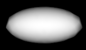
a) b)

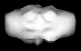
Figure 2.— Example of artifical shape used as a test object to be fitted for. a) The initial shape, a prolate ellipsoid, before any of the spherical harmonic parameters have been changed. b) A perturbed prolate ellipsoid.

For each test case, we then generated between 20 and 30 simulated radar images and added Gaussian noise such that pixel values on the target exceed the root-mean-square (rms) deviations of the noise by an average factor of $\sim 5$ and a peak factor of $\sim 150$. These images were used to attempt to reconstruct the perturbed shape, with the original basic shape (sphere, prolate ellipsoid, or oblate ellipsoid) given as the initial condition. This process was repeated for each of the nine test cases.

The three fitting algorithms shared the same starting conditions for each test. For each fit, the models comprised 121 free parameters (corresponding to the coefficients of a ten-degree spherical harmonic representation), and the simulated images contained a total of 2.4 million data points. Stopping criteria were also normalized for the three different test types – a fit was considered finished if the $\chi^{2}$ statistic had not changed to within three significant digits after one hour, or twelve hours had passed since the fit began, whichever occurred first. Time-based stopping criteria – as opposed to iteration-based – were chosen in order to account for fundamental differences between the algorithms with respect to the definition of a single iteration. In addition, fits were allowed to run past the criteria stopping point, and the criteria were analyzed and applied afterwards. This was to avoid missing a drop-off in $\chi^{2}$ in one test type that might not appear in another. All times are wall clock time.

The results of these tests (figure 3) indicate that SRIF consistently performs better than the currently-used SPF algorithm. In addition, SRIF appears to ultimately converge on a lower chi-squared than LM in all cases.

SRIF also converged on a reduced chi-squared ($\chi_{red}^{2}$) of less than 1.3 (indicating a reasonable approximation of the correct model parameters had been found) in eight out of the nine tests, while SPF was only able to do so in one out of the nine tests.

V.2. Simulated data with existing asteroid shape models

We conducted another set of tests using existing shape models of asteroids. Three cases were tested - Itokawa, the 1999 KW4 primary, and 2000 ET70 (figure 4). As opposed to the previous set of tests, these shapes are not guaranteed to be well approximated with a spherical harmonic representation. However, a best-fit spherical harmonic representation can still be found.

For this set of images we used $\chi^{2}$-distributed errors, which is the correct noise model for individual images of radar echo power. We chose a noise model such that the pixel values on the target exceed the rms deviations of the noise by an average factor of $\sim 2$ and a peak factor of $\sim 60$. When multiple images are summed, one can often rely on the fact that errors approach normality by the central limit theorem, hence the choice of Gaussian noise for the images tested in section V.1.

The results of these tests are illustrated in figure 5, and an example comparison of a fit synthetic image to the simulated image is shown in figure 6. Our implementation of SRIF clearly performs faster and with higher accuracy than both SPF and LM.

V.3. Spin state

Jointly solving for spin state and shape is typically challenging and time-consuming with the traditional implementation of shape. A common approach is to estimate the spin state as best as possible with rudimentary shapes (e.g., ellipsoids or low-order spherical harmonic models) in a basic grid search. One can then use the most favorable trial values of the spin state to fit a model for the physical shape to the observed radar images. Experience with traditional shape indicates that the algorithm rarely deviates much from the initial conditions given on the spin state, probably as a result of the one-parameter-at-a-time fitting approach.

Our tests indicate that SRIF is capable of fitting a reasonable asteroid shape, even when the initial shape and spin state parameters are far away from their optimal values. This advantage likely results from the joint estimation of shape and spin parameters.

For example, figure 7 shows the best-fit spherical harmonics shape, as determined by SRIF, for a set of simulated images of the asteroid Itokawa. The initial conditions for the shape parameters were a sphere with a radius $10\%$ larger than the longest axis of the actual shape model. In addition, the initial spin axis was $30$ degrees off from the spin axis with which the data were simulated. We repeated these experiments with a variety of starting conditions, as well as several different shape models, with similar results.

SRIF’s capacity to fit for both shape and spin state parameters can drastically cut down on the total time required to obtain an accurate asteroid shape model.

V.4. Real data: 2000 ET70

We have run shape with all three fitting algorithms on actual radar images of the asteroid 2000 ET70 (Naidu et al., 2013). shape was run initially with an ellipsoid model. The starting conditions for this model were such that the ellipsoid axes were all equal. The best fit ellipsoid model ($a/b=1.16,b/c=1.13$) was then converted into a spherical harmonic model with 122 model components (corresponding to the coefficients of a ten-degree spherical harmonic representation, as well as one overall size scaling factor), which was then fit again to the data. This process resulted in a final spherical harmonic model (figure 8) for the asteroid with a $\chi_{red}^{2}$ of 2.1. The stopping criterion was a reduction in $\chi_{red}^{2}$ less than 0.01 between two consecutive iterations.

For the first stage, SRIF fit a substantially better ellipsoid than SPF did, although it took about eight minutes longer (Table 1). For the second stage, SRIF converged on a final solution more than two times faster than SPF. This further corroborates the results obtained from our tests with simulated data.

Table 1Run statistics for SPF and SRIF fits for 2000 ET70 data.

Model	$\chi^{2}_{initial}$	$\chi_{final}^{2}$			Runtime (hours)
		SPF	LM	SRIF	SPF	LM	SRIF
2000 ET70: Ellipsoid	3.7	2.8	2.7	2.4	0.02	0.84	0.129
2000 ET70: Sph. Harm.	2.4	2.10	2.37	2.10	2.98	0.1725	1.36

VI. Future changes

The addition of SRIF to shape has improved fitting performance, but additional changes can still be made to allow shape to function optimally with real-world data.

VI.1. Global vs local variable partitioning

The fits discussed in this paper were performed on global parameters only – namely, parameters that are valid across all data sets associated with the object in question. When performing a high-fidelity fit on multiple data sets, however, it is necessary to take into account local parameters as well. These are model arguments which apply only at specific points in time. For example, while the mean radius and rotation rate of an asteroid is a global parameter, the system temperature and ephemeris correction parameters on the third day of observations are local to the data taken on the third day of observations.

Processing local parameters is less computationally intensive than processing global parameters. The gradients of any observables not within a local parameter’s timeframe are known a priori to be zero. This greatly reduces the number of modelling function calls that must be made when considering local parameters. In addition, the triangularization of a derivative matrix scales with the number of non-zero elements. This means that while the total number of additional parameters scales like the product of the number of datasets with the average number of local parameters per dataset, the additional computation time only scales with the average number of local parameters per data set. Because of this, adding the capacity for processing local parameters will only increase runtime by ${\sim}20\%$. We plan on adding this functionality in a future version of shape.

VI.2. Additional fitting methods

Tests that we have run with the simulated and real data have indicated that the $\chi^{2}$-space for shape-models is not smooth. Figure 9 shows a two-dimensional slice of the $\chi^{2}$-space for a spherical harmonic model against 2000 ET70 data. The multi-valleyed nature of this space makes it difficult for local fitting methods to find the global minimum. In light of this, global fitting mechanisms such as simulated annealing or Markov Chain Monte Carlo may be better suited for this problem. These methods can be supplemented by a gradient descent method like SRIF. In fact, utilizing a hybrid of these methods may prove to be the optimal solution for this class of problem. Until such methods are implemented, convergence on a global minimum will be dependent on a good choice of starting conditions. This often forces shape modelers to explore a variety of initial conditions, and identifying such starting conditions is not always practical.

VI.3. Additional shape representations

There are serious drawbacks to using spherical harmonics to represent the radius of an object at each latitude-longitude grid point. Many asteroid shapes are poorly approximated by this representation (e.g., the 1999 KW4 primary) and there are entire classes of shapes (e.g., banana) that can not be described at all in this fashion. Traditionally, this problem has been solved by the use of vertex models, but these shape representations typically involve a large number of parameters (i.e., the coordinates of three vertices per facet). We are currently looking into new representation methods, some of which may allow for a greater range of shapes, while at the same time cutting down on the number of free parameters.

VII. Conclusions

We have added new optimization procedures into the asteroid shape modeling software shape, enabling the use of a Levenberg-Marquardt algorithm or a Square Root Information Filter. We implemented several optimizations to the SRIF algorithm to increase performance in shape inversion problems. Tests on both simulated and actual data indicate that our additions allow shape inversion to proceed more quickly and with better fidelity than was previously possible. The SRIF implementation also facilitates simultaneous fits of the spin axis orientation and shape.

Appendix A Numerical Stability

Issues with numerical stability can arise when multiplying matrices with elements at or near the square root of the machine precision. This can lead to erroneous results, or singular matrices for which further calculations (such as the matrix inverse) are impossible.

For example (Bierman, G. J., 1977), consider the case when

$$A=\left(\begin{array}[]{c c}1&1-\epsilon\\ 1-\epsilon&1\\ 1&1\end{array}\right)$$

and

$$W=I.$$

Then

$$(A^{\intercal}WA)=\left(\begin{array}[]{c c}3-2\epsilon+\epsilon^{2}&3-2\epsilon\\ 3-2\epsilon&3-2\epsilon+\epsilon^{2}\end{array}\right)$$

Thus, in the case that $\epsilon$ is equal to or less than the square root of the machine precision,

$$(A^{\intercal}WA)=\left(\begin{array}[]{c c}3-2\epsilon&3-2\epsilon\\ 3-2\epsilon&3-2\epsilon\end{array}\right).$$

This matrix is singular, and thus $(A^{\intercal}WA)^{-1}$ cannot be computed. This problem is particularly insidious because matrix singularity in higher dimensions can be difficult to detect.

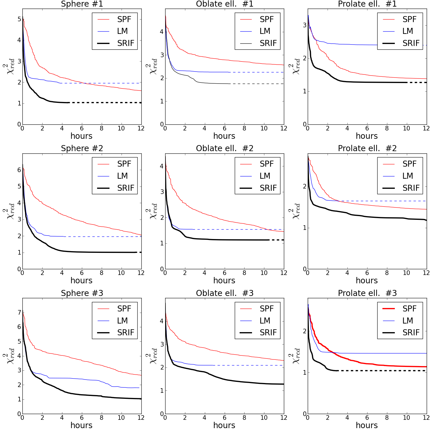
Figure 3.— Results of three fitting algorithms (Sequential Parameter Fit, Levenberg-Marquardt, and Square-Root Information Filter) with three artificial shapes (perturbed versions of a sphere, oblate ellipsoid, and prolate ellipsoid). Bold lines indicate fits which converged to a $\chi^{2}_{red}<1.3$. Dashed lines indicate the assumed future state for fits that had converged on a solution before the 12-hour time frame.

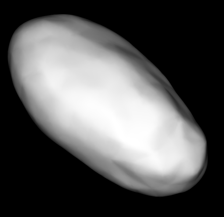
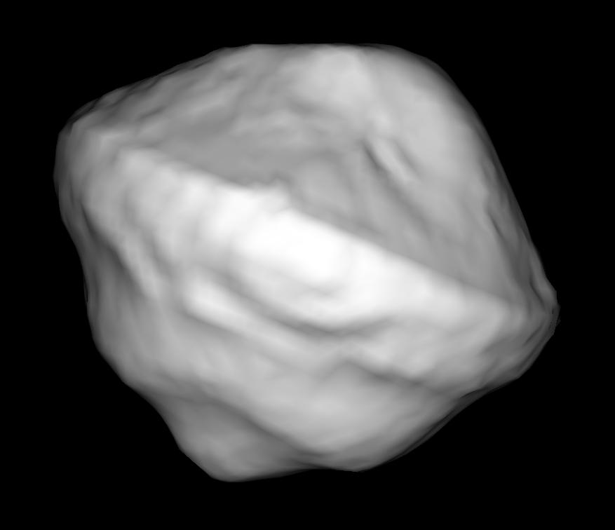
a) b) c)

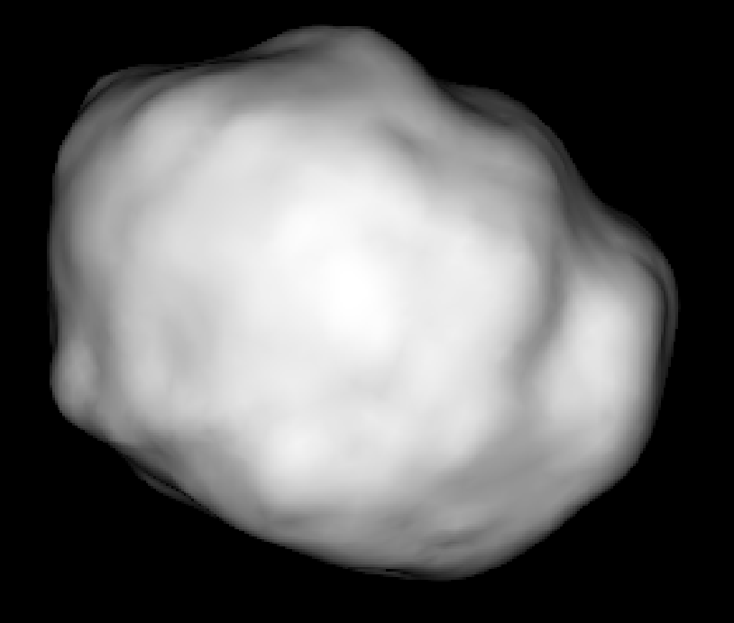
Figure 4.— Plane of sky representations of the radar-derived shape models of (a) Itokawa, (b) 1999 KW4, and (c) 2000 ET70 .

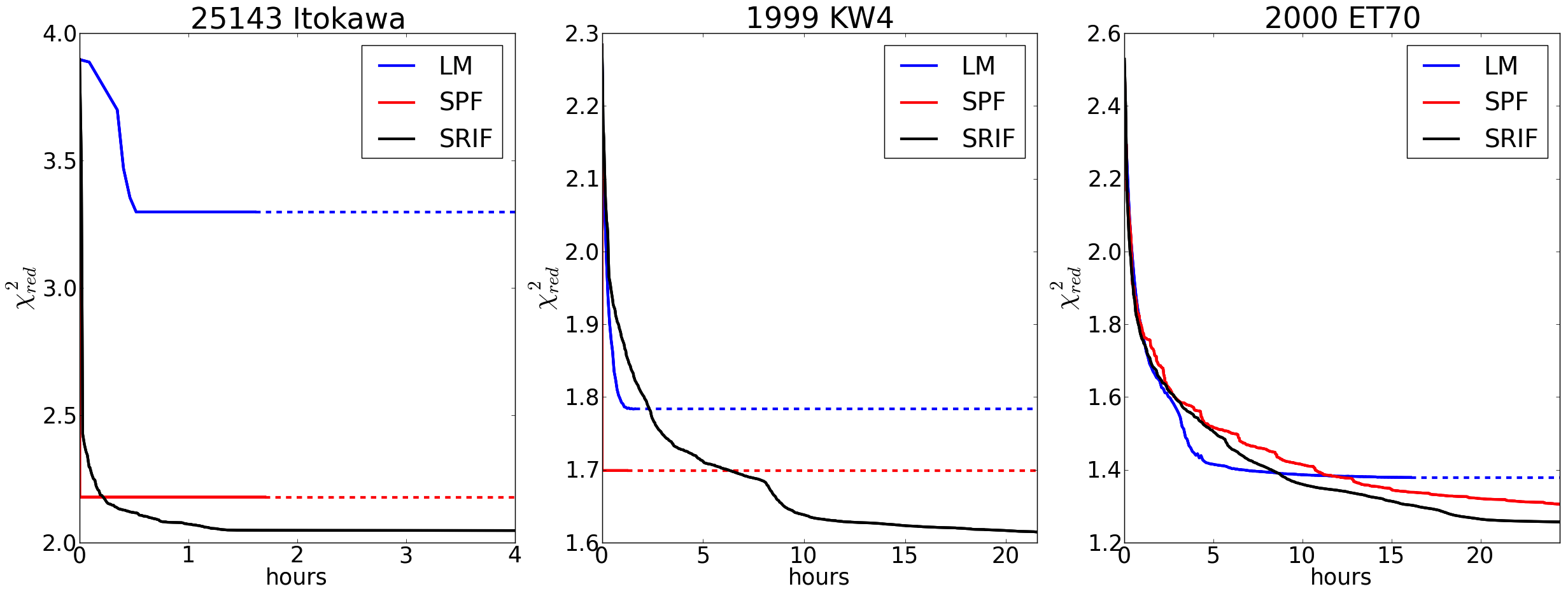
Figure 5.— Results comparing SRIF, LM, and SPF operating on real asteroid shapes with simulated $\chi^{2}$-distributed errors. Dashed lines indicate the assumed future state for fits that had converged on a solution. These fits were run without penalty functions. Note that the solution arrived at by SPF for 1999 KW4 was a non-physical, pebble-sized asteroid. Avoiding non-physical minima in the $\chi^{2}$ space would require human intervention to manually tweak the starting conditions. We did not perform such tweaks in order to maintain consistency in our tests.

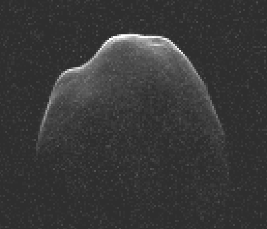
a) b)

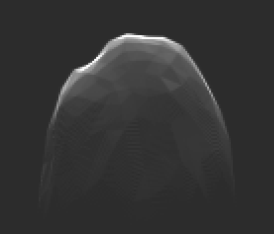
Figure 6.— (a) Example of a simulated input to the shape modeling algorithm. The input is generated by projecting the shape model into range-Doppler space at a specific observation epoch and adding random noise. (b) The corresponding synthetic image produced by the shape modeling algorithm after fitting for the shape.

a)

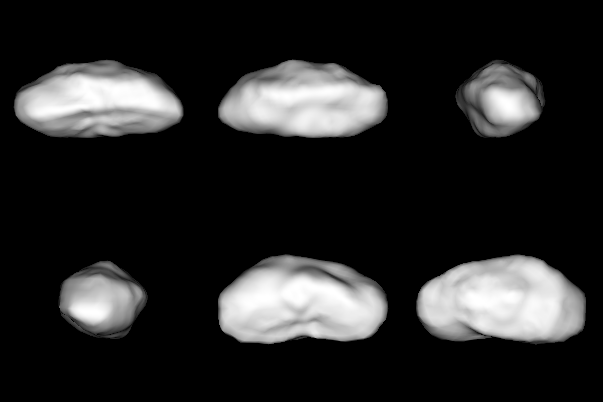
b)

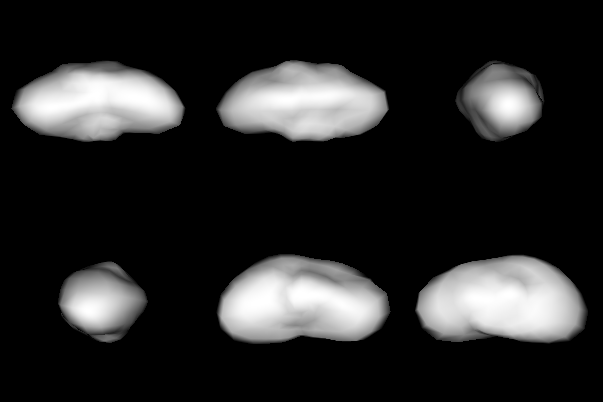
Figure 7.— a) The Itokawa shape model that was used to generate simulated radar images (Ostro et al., 2005). b) The best-fit SRIF tenth degree spherical-harmonics model for those simulated data, using penalty functions. The initial conditions for the shape parameters were a sphere with an offset spin axis latitude and longitude.

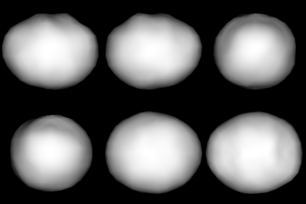
Figure 8.— The best SRIF fit spherical harmonic model for 2000 ET70, which is in good agreement with the model of Naidu et al. (2013).

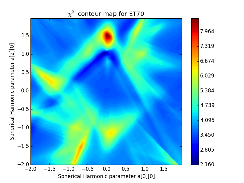
Figure 9.— A two-dimensional slice of the $\chi^{2}$ space for fitting shape models to radar data. This contour map represents $\chi^{2}$ for a spherical harmonic model with all parameters fixed except two of the elements of the primary coefficient matrix. Note that the blue regions indicate low $\chi^{2}$, and that there are several of these regions for a derivative-based optimizer to fall towards, depending on the initial set of starting conditions.

References

- Benner et al. (2008) Benner, L. A. M., Nolan, M. C., Margot, J. L., et al. 2008, in Bulletin of the American Astronomical Society, Vol. 40, AAS/Division for Planetary Sciences Meeting Abstracts #40, 432
- Bierman, G. J. (1977) Bierman, G. J. 1977, ”Factorization Methods for Discrete Sequential Estimation” (Dover)
- Bottke et al. (2006) Bottke, Jr., W. F., Vokrouhlický, D., Rubincam, D. P., & Nesvorný, D. 2006, Annual Review of Earth and Planetary Sciences, 34, 157
- Chesley et al. (2014) Chesley, S. R., Farnocchia, D., Nolan, M. C., et al. 2014, Icarus, 235, 5
- Ćuk & Nesvorný (2010) Ćuk, M., & Nesvorný, D. 2010, Icarus, 207, 732
- Fahnestock & Scheeres (2009) Fahnestock, E. G., & Scheeres, D. J. 2009, Icarus, 201, 135
- Farnocchia et al. (2013) Farnocchia, D., Chesley, S. R., Chodas, P. W., et al. 2013, Icarus, 224, 192
- Fujiwara et al. (2006) Fujiwara, A., Kawaguchi, J., Yeomans, D. K., et al. 2006, Science, 312, 1330
- Giorgini et al. (2002) Giorgini, J. D., Ostro, S. J., Benner, L. A. M., et al. 2002, Science, 296, 132
- Harris et al. (2009) Harris, A. W., Fahnestock, E. G., & Pravec, P. 2009, Icarus, 199, 310
- Hudson (1993) Hudson, R. S. 1993, Remote Sensing Reviews, 8, 195
- Hudson & Ostro (1994) Hudson, R. S., & Ostro, S. J. 1994, Science, 263, 940
- Hudson & Ostro (1995) —. 1995, Science, 270, 84
- Jacobson et al. (2014) Jacobson, S. A., Scheeres, D. J., & McMahon, J. 2014, ApJ, 780, 60
- Lawson & Hanson (1995) Lawson, C. L., & Hanson, R. J. 1995, SIAM Classics in Applied Mathematics, Vol. 15, ”Solving Least Squares Problems” (Philadelphia: Society for Industrial and Applied Mathematics)
- Lowry et al. (2007) Lowry, S. C., Fitzsimmons, A., Pravec, P., et al. 2007, Science, 316, 272
- Magri et al. (2007) Magri, C., Ostro, S. J., Scheeres, D. J., et al. 2007, Icarus, 186, 152
- Margot et al. (2002) Margot, J. L., Nolan, M. C., Benner, L. A. M., et al. 2002, Science, 296, 1445
- Margot et al. (2015) Margot, J. L., Pravec, P., Taylor, P. A., Carry, B., & Jacobson, S. A. 2015, in Asteroids IV, in press
- Naidu & Margot (2015) Naidu, S. P., & Margot, J. L. 2015, AJ, 149, 80
- Naidu et al. (2013) Naidu, S. P., Margot, J. L., Busch, M. W., et al. 2013, Icarus, 226, 323
- Nolan et al. (2013) Nolan, M. C., Magri, C., Howell, E. S., et al. 2013, Icarus, 226, 629
- Nugent et al. (2012) Nugent, C. R., Margot, J. L., Chesley, S. R., & Vokrouhlický, D. 2012, Astronomical Journal, 144, 60
- Ostro et al. (1995) Ostro, S., Hudson, R., Jurgens, R., et al. 1995, Science, 270, 80+
- Ostro (1993) Ostro, S. J. 1993, Reviews of Modern Physics, 65, 1235
- Ostro et al. (2005) Ostro, S. J., Benner, L. A. M., Magri, C., et al. 2005, Meteoritics and Planetary Science, 40, 1563
- Ostro et al. (2006) Ostro, S. J., Margot, J. L., Benner, L. A. M., et al. 2006, Science, 314, 1276
- Pravec et al. (2002) Pravec, P., Harris, A. W., & Michalowski, T. 2002, in Asteroids III (Univ. of Arizona Press), 113–122
- Press et al. (1992) Press, W. H., Teukolsky, S. A., Vetterling, W. T., & Flannery, B. P. 1992, Numerical Recipes in C (2nd Ed.): The Art of Scientific Computing (New York, NY, USA: Cambridge University Press)
- Scheeres et al. (2006) Scheeres, D. J., Fahnestock, E. G., Ostro, S. J., et al. 2006, Science, 314, 1280
- Takahashi & Scheeres (2014) Takahashi, Y., & Scheeres, D. J. 2014, Celestial Mechanics and Dynamical Astronomy, 119, 169
- Taylor et al. (2007) Taylor, P. A., Margot, J. L., Vokrouhlický, D., et al. 2007, Science, 316, 274
- Vokrouhlický et al. (2000) Vokrouhlický, D., Milani, A., & Chesley, S. R. 2000, Icarus, 148, 118