Connectivity in Secure Wireless Sensor Networks
under Transmission Constraints

Abstract

In wireless sensor networks (WSNs), the Eschenauer–Gligor (EG) key pre-distribution scheme is a widely recognized way to secure communications. Although the connectivity properties of secure WSNs with the EG scheme have been extensively investigated, few results address physical transmission constraints. These constraints reflect real–world implementations of WSNs in which two sensors have to be within a certain distance from each other to communicate. In this paper, we present the first zero–one laws for connectivity in WSNs employing the EG scheme under transmission constraints. These laws improve recent results [10, 11] significantly, are sharp, and help specify the critical transmission ranges for connectivity. Our analytical findings, which are also confirmed via numerical experiments, provide precise guidelines for the design of secure WSNs in practice. The application of our theoretical results to frequency hopping of wireless networks is discussed in some detail.

1 INTRODUCTION

The Eschenauer–Gligor key pre-distribution scheme [7] is regarded as a typical approach to secure communications in wireless sensor networks (WSNs). In this scheme (referred to as the EG scheme hereafter), each sensor is independently assigned the same number of distinct cryptographic keys selected uniformly at random from a key pool before deployment. After deployment, any two sensors establish a link between them, if they share at least one key.

Connectivity in secure WSNs employing the EG scheme has been extensively studied in the literature [2, 18, 17, 22, 10, 11]. However, most existing research [2, 18, 17, 22] unrealistically assumes unconstrained sensor-to-sensor communications; i.e., any two sensors can communicate regardless of the distance between them. Only two recent results [10, 11] take transmission constraints into consideration, but do not provide zero–one laws for connectivity.

In this paper, we establish the first and also sharp zero–one laws for connectivity in WSNs using the EG scheme under practical transmission constraints. We present significantly improved conditions for asymptotic connectivity over those of Krishnan et al. [10] and Krzywdziński and Rybarczyk [11], and also demonstrate that as the parameters move further away from these conditions, the network rapidly becomes asymptotically disconnected. Our results provide useful guidelines for dimensioning the EG scheme and adjusting sensor transmission power to ensure network connectivity. Moreover, our zero–one laws enable us to determine the critical transmission ranges for connectivity. Intuitively, as the transmission range surpasses (resp., falls below) the critical value and grows (resp., declines) further, the network immediately enters an asymptotically connected (resp., disconnected) state.

To model transmission constraints, we use the popular disk model [14, 8, 13, 12, 20], in which each sensor’s transmission area is a disk with a uniform distance as its radius; i.e., two sensors have to be within the radius distance to communicye directly. The network area in our analysis is either a torus or a square. The square accounts for the real–world boundary effect whereby some transmission region of a sensor close to the network boundary may falls outside the network field. In contrast, the torus eliminates the boundary effect.

The rest of the paper is organized as follows. In Section 2, we describe the system model. Section 3 presents the main results, leading to the discussion of critical transmission ranges in Section 4. Afterwards, we explain the practicality of theorems’ conditions in Section 5. We provide numerical experiments in Section 6. In Section 7, we discuss the application of our results to frequency hopping in detail. Section 8 reviews related work; and Section 9 concludes the paper. The Appendix contains the zero–law proofs and the sketch of the (simpler) one–law proofs.

2 SYSTEM MODEL

In a WSN with size $n$ and sensor set $\mathcal{V}=\{v_{1},v_{2},\ldots,v_{n}\}$, the EG scheme independently assigns a set of $K_{n}$ distinct cryptographic keys, which are selected uniformly at random from a pool of $P_{n}$ keys, to each sensor node. The set of keys of each sensor is called the key ring and is denoted by $S_{x}$ for sensor $v_{x}$. The EG scheme is modeled by a random key graph [17, 22, 10], denoted by $G_{RKG}(n,K_{n},P_{n})$ in which an edge exists between two nodes $v_{x}$ and $v_{y}$ if and only if they possess at least one common key; i.e., the event $[S_{x}\hskip 2.0pt{\cap}\hskip 2.0ptS_{y}\neq\emptyset]$, denoted by $K_{xy}$, holds. As for the sensor distribution, we consider that the $n$ nodes are independently and uniformly deployed in a network area $\mathcal{A}$. The disk model induces a random geometric graph [14, 10, 11, 13, 8, 20], denoted by $G_{RGG}(n,r_{n},\mathcal{A})$, in which an edge exists between two sensors if and only if their distance is no greater than $r_{n}$. In a secure WSN using the EG scheme under the disk model, two sensors $v_{x}$ and $v_{y}$ establish a direct link between them if and only if they share at least one key and are within distance $r_{n}$. We denote the event establishing this direct link by $E_{xy}$. If we let graph $G(n,\theta_{n},\mathcal{A})$ model such a WSN, it is straightforward to see $G(n,\theta_{n},\mathcal{A})$ is the intersection of random key graph $G_{RKG}(n,K_{n},P_{n})$ and random geometric graph $G_{RGG}(n,r_{n},\mathcal{A})$; namely,

$$G(n,\theta_{n},\mathcal{A}) =G_{RKG}(n,K_{n},P_{n})\hskip 2.0pt{\cap}\hskip 2.0ptG_{RGG}(n,r_{n},\mathcal{A}),$$

where parameters $K_{n},P_{n}$ and $r_{n}$ are together represented by $\theta_{n}$. Also, if we let region $\mathcal{A}$ be either a torus $\mathcal{T}$ or a square $\mathcal{S}$, each with a unit area, we obtain the two graphs

$$G(n,\theta_{n},\mathcal{T}) =G_{RKG}(n,K_{n},P_{n})\hskip 2.0pt{\cap}\hskip 2.0ptG_{RGG}(n,r_{n},\mathcal{T}),$$

and

$$G(n,\theta_{n},\mathcal{S}) =G_{RKG}(n,K_{n},P_{n})\hskip 2.0pt{\cap}\hskip 2.0ptG_{RGG}(n,r_{n},\mathcal{S}).$$

We let $p_{s}$ be the probability of key sharing between two sensors and note that $p_{s}$ is also the edge probability in random key graph $G_{RKG}(n,K_{n},P_{n})$. It holds that $p_{s}=\mathbb{P}[{K}_{xy}]=\mathbb{P}[S_{x}\cap S_{y}\neq\emptyset]$. Clearly, if $P_{n}<2K_{n}$, then $p_{s}=1$. If $P_{n}\geq 2K_{n}$, as shown in previous work [2, 17, 22], we have $p_{s}=1-{\binom{P_{n}-K_{n}}{K_{n}}}\big{/}{\binom{P_{n}}{K_{n}}}$. If $P_{n}\geq 2K_{n}$, by [3, Lemma 6], it further holds that

$$p_{s} \leq{{K_{n}}^{2}}/{P_{n}}.$$ (1)

By [24, Lemma 8], (1) implies that if ${{K_{n}}^{2}}/{P_{n}}=o(1)$, then

$$p_{s} ={{K_{n}}^{2}}/{P_{n}}\cdot\big{[}1-O\big{(}{{K_{n}}^{2}}/{P_{n}}\big{)}\big{]}\sim{{K_{n}}^{2}}/{P_{n}}.$$ (2)

We will frequently use (1) and (2) throughout the paper.

Let $p_{e}$ be the probability that a link exists between two sensors in the WSN modeled by graph $G(n,\theta_{n},\mathcal{A})$; i.e., $p_{e}$ is the edge probability in $G(n,\theta_{n},\mathcal{A})$. It holds that $p_{e}=\mathbb{P}[E_{xy}]$. When $\mathcal{A}$ is the torus $\mathcal{T}$, clearly $p_{e}$ equals $\pi{r_{n}}^{2}\cdot p_{s}$; and if ${{K_{n}}^{2}}/{P_{n}}=o(1)$, then $p_{e}\sim\pi{r_{n}}^{2}\cdot{{K_{n}}^{2}}/{P_{n}}$ by (2). When $\mathcal{A}$ is the square $\mathcal{S}$, it is a simple matter to show $p_{e}\leq\pi{r_{n}}^{2}\cdot p_{s}$ and $p_{e}\geq(1-2{r_{n}})^{2}\cdot\pi{r_{n}}^{2}\cdot p_{s}$, yielding $p_{e}\sim\pi{r_{n}}^{2}\cdot p_{s}$ if $r_{n}=o(1)$. Therefore, on $\mathcal{S}$, if $r_{n}=o(1)$ and ${{K_{n}}^{2}}/{P_{n}}=o(1)$, we further obtain $p_{e}\sim\pi{r_{n}}^{2}\cdot{{K_{n}}^{2}}/{P_{n}}$ in view of (2).

In addition to random key graphs and random geometric graphs, the Erdős-Rényi graph [6] has also been extensively studied. An Erdős–Rényi graph $G_{ER}(n,p_{n})$ is defined on a set of $n$ nodes such that any two nodes establish an edge in between independently with probability $p_{n}$. As already shown in the literature [2, 17, 18, 22], random key graph $G_{RKG}(n,K_{n},P_{n})$ and Erdős-Rényi graph $G_{ER}(n,p_{n})$ have similar connectivity properties when they are matched through edge probabilities; i.e. when $p_{s}=p_{n}$. Hence, it would be tempting to exploit this analogy and conclude that connectivity in $G(n,\theta_{n},\mathcal{A})$ (i.e., $G_{RKG}(n,K_{n},P_{n})\hskip 2.0pt{\cap}\hskip 2.0ptG_{RGG}(n,r_{n},\mathcal{A})$) is similar to that of $G_{ER}(n,p_{n})\hskip 2.0pt{\cap}\hskip 2.0ptG_{RGG}(n,r_{n},\mathcal{A})$, which was recently established [15]. However tempting, such heuristic approaches do not work as graphs $G_{ER}(n,p_{s})$ and $G_{RKG}(n,K_{n},P_{n})$ (and their respective intersections) are quite different. For instance, in $G_{ER}(n,p_{s})$, for any three nodes $v_{x},v_{y}$ and $v_{z}$, the event that $v_{x}$ has edges with both $v_{y}$ and $v_{z}$, is independent of the event that $v_{y}$ and $v_{z}$ has an edge between them. However, in $G_{RKG}(n,K_{n},P_{n})$, these two events are not independent from each other, since the event that $v_{x}$ has edges with both $v_{y}$ and $v_{z}$ means that the key rings $S_{y}$ and $S_{z}$ of $v_{y}$ and $v_{z}$ respectively both have intersections with the key ring $S_{x}$ of $v_{x}$. This has an impact on whether $S_{y}$ and $S_{z}$ intersects. In fact, it has been formally proven [22, 3] that graphs $G_{ER}(n,p_{s})$ and $G_{RKG}(n,K_{n},P_{n})$ exhibit different characteristics in terms of properties including clustering coefficient, number of triangles, etc.

3 THE MAIN RESULTS

We detail the main results below. The notation “$\ln$” stands for the natural logarithm function.

3.1 Connectivity in a Secure WSN on a Torus

Theorem 1 presents a zero–one law for connectivity in $G(n,\theta_{n},\mathcal{T})$, which models a secure WSN working under the EG scheme and the disk model on a unit torus.

Theorem 1.

Let graph $G(n,\theta_{n},\mathcal{T})$ be the intersection of random key graph $G_{RKG}(n,K_{n},P_{n})$ and random geometric graph $G_{RGG}(n,r_{n},\mathcal{T})$ on a unit torus $\mathcal{T}$, where there exist some $\mu_{n}=\omega(1)$ and constant $c_{1}$ such that

$$\max\bigg{\{}\frac{\ln n}{\ln\ln n},\hskip 1.5pt\mu_{n}\cdot\sqrt{\frac{P_{n}\ln n}{n}}\bigg{\}} \leq K_{n}\leq c_{1}\sqrt{\frac{P_{n}}{\ln n}}$$ (3)

for all $n$ sufficiently large. For all $n$, let the sequence $\alpha_{n}$ be defined through

$$\pi{r_{n}}^{2}\cdot\frac{{K_{n}}^{2}}{P_{n}} =\frac{\ln n+\alpha_{n}}{n}.$$ (4)

Then

$$\lim\limits_{n\to\infty}\mathbb{P}\left[\begin{array}[]{l}\textrm{$G(n,\theta_{n},\mathcal{T})$}\\ \textrm{is connected.}\end{array}\right] =\begin{cases}0,~{}~{}\textrm{if $\lim\limits_{n\to\infty}{\alpha_{n}}=-\infty$},\\ 1,~{}~{}\textrm{if $\lim\limits_{n\to\infty}{\alpha_{n}}=\infty$}.\end{cases}$$ (7)

Remark 1.

Under (3), we obtain $\frac{{K_{n}}^{2}}{P_{n}}\leq\frac{{c_{1}}^{2}}{\ln n}=o(1)$. Then as noted in Section 2, $\pi{r_{n}}^{2}\cdot\frac{{K_{n}}^{2}}{P_{n}}$ in (4) asymptotically equals the edge probability in graph $G(n,\theta_{n},\mathcal{T})$.

3.2 Connectivity in a Secure WSN on a Square

Theorem 2 gives a zero–one law for connectivity in $G(n,\theta_{n},\mathcal{S})$, which models a secure WSN working under the EG scheme and the disk model on a unit square.

Theorem 2.

Let graph $G(n,\theta_{n},\mathcal{S})$ be the intersection of random key graph $G_{RKG}(n,K_{n},P_{n})$ and random geometric graph $G_{RGG}(n,r_{n},\mathcal{S})$ on a unit square $\mathcal{S}$, where there exist some constants $c_{2}>0,$ $0<c_{3}<1$, $c_{4}>0$ and $\nu_{n}=o(1)$ such that

$$c_{2}\sqrt{\frac{P_{n}\ln n}{n^{c_{3}}}} \leq K_{n}\leq\min\Bigg{\{}\nu_{n}\cdot\sqrt{\frac{P_{n}}{\ln n}},\hskip 1.5pt{\frac{c_{4}P_{n}}{n\ln n}}\hskip 2.0pt\Bigg{\}}$$ (8)

for all $n$ sufficiently large. Assume that $\frac{{K_{n}}^{2}}{P_{n}}\cdot n^{1/3}\ln n$ either is bounded for all $n$ or converges to $\infty$ as $n\to\infty$, and for all $n$ let the sequence $\alpha_{n}$ be defined through

$$\pi{r_{n}}^{2}\cdot\textrm{ $\frac{{K_{n}}^{2}}{P_{n}}$}$$

$$=\begin{cases}\textrm{ $\frac{\ln\frac{nP_{n}}{{K_{n}}^{2}}\hskip 2.0pt-\hskip 2.0pt\ln\ln\frac{nP_{n}}{{K_{n}}^{2}}\hskip 2.0pt+\hskip 2.0pt\alpha_{n}}{n}$},&\textrm{for~{}}\textrm{\large$\frac{{K_{n}}^{2}}{P_{n}}$}=\omega\textrm{\large$\left(\frac{1}{n^{1/3}\ln n}\right)$},\\ \vspace{-7pt}\\ \textrm{ $\frac{4\ln\frac{P_{n}}{{K_{n}}^{2}}\hskip 2.0pt-\hskip 2.0pt4\ln\ln\frac{P_{n}}{{K_{n}}^{2}}\hskip 2.0pt+\hskip 2.0pt\alpha_{n}}{n}$},&\textrm{for~{}}\textrm{\large$\frac{{K_{n}}^{2}}{P_{n}}$}=O\textrm{\large$\left(\frac{1}{n^{1/3}\ln n}\right)$}.\end{cases}$$ (9)

Then

$$\lim\limits_{n\to\infty}\mathbb{P}\left[\begin{array}[]{l}\textrm{$G(n,\theta_{n},\mathcal{S})$}\\ \textrm{is connected.}\end{array}\right] =\begin{cases}0,~{}~{}\textrm{if $\lim\limits_{n\to\infty}{\alpha_{n}}=-\infty$},\\ 1,~{}~{}\textrm{if $\lim\limits_{n\to\infty}{\alpha_{n}}=\infty$.}\end{cases}$$ (12)

Remark 2.

Under (8), we have $\frac{{K_{n}}^{2}}{P_{n}}\leq\frac{{\nu_{n}}^{2}}{\ln n}=o(1)$. If it further holds $r_{n}=o(1)$ (this is true with confined $\alpha_{n}$), then as established in Section 2, $\pi{r_{n}}^{2}\cdot\frac{{K_{n}}^{2}}{P_{n}}$ in (9) asymptotically equals the edge probability in graph $G(n,\theta_{n},\mathcal{S})$.

4 CRITICAL TRANSMISSION RANGES

4.1 The Critical Transmission Range for Connectivity in a Secure WSN on a Unit Torus

By Theorem 1, under condition (3), we can determine the critical transmission range $r_{n}^{*}(\mathcal{T})$ for connectivity in a secure WSN on a unit torus modeled by graph $G(n,\theta_{n},\mathcal{T})$ through

$$\pi\big{[}{r_{n}^{*}(\mathcal{T})}\big{]}^{2}\cdot\frac{{K_{n}}^{2}}{P_{n}} =\frac{\ln n}{n},$$

inducing the following expression of $r_{n}^{*}(\mathcal{T})$:

$$r_{n}^{*}(\mathcal{T})=\sqrt{\frac{\ln n}{\pi n}\cdot\frac{P_{n}}{{K_{n}}^{2}}}.$$ (13)

By (13), it is clear that with $n$ fixed, $r_{n}^{*}(\mathcal{T})$ decreases as $\frac{{K_{n}}^{2}}{P_{n}}$ increases. This is expected since as mentioned in Remark 1 after Theorem 1, $\frac{{K_{n}}^{2}}{P_{n}}$ asymptotically equals the probability that two sensors share at least one key; and $\pi{r_{n}}^{2}\cdot\frac{{K_{n}}^{2}}{P_{n}}$ asymptotically equals the edge probability in $G(n,\theta_{n},\mathcal{T})$. As the probability of key sharing increases, sensors can reduce their transmission ranges to maintain network connectivity.

We explain $r_{n}^{*}(\mathcal{T})=o(1)$, which is anticipated as the node density $n$ grows to $\infty$. From $K_{n}\geq\sqrt{\frac{P_{n}\ln n}{n}}\cdot\mu_{n}$ in (3), where $\mu_{n}=\omega(1)$, it follows that $\frac{{K_{n}}^{2}}{P_{n}}=\omega\big{(}\frac{\ln n}{n}\big{)}$, which along with (13) leads to $r_{n}^{*}(\mathcal{T})=o(1)$.

4.2 The Critical Transmission Range for Connectivity in a Secure WSN on a Unit Square

By Theorem 2, under condition (8), we can determine the critical transmission range $r_{n}^{*}(\mathcal{S})$ for connectivity in a secure WSN on a unit square modeled by graph $G(n,\theta_{n},\mathcal{S})$ through

$$\pi\big{[}{r_{n}^{*}(\mathcal{S})}\big{]}^{2}\cdot\frac{{K_{n}}^{2}}{P_{n}}$$

$$=\begin{cases}\textrm{ $\frac{\ln\frac{nP_{n}}{{K_{n}}^{2}}\hskip 2.0pt-\hskip 2.0pt\ln\ln\frac{nP_{n}}{{K_{n}}^{2}}\hskip 2.0pt}{n}$},&\textrm{for~{}}\textrm{\large$\frac{{K_{n}}^{2}}{P_{n}}$}=\omega\textrm{\large$\left(\frac{1}{n^{1/3}\ln n}\right)$},\\ \vspace{-7pt}\\ \textrm{ $\frac{4\ln\frac{P_{n}}{{K_{n}}^{2}}\hskip 2.0pt-\hskip 2.0pt4\ln\ln\frac{P_{n}}{{K_{n}}^{2}}\hskip 2.0pt}{n}$},&\textrm{for~{}}\textrm{\large$\frac{{K_{n}}^{2}}{P_{n}}$}=O\textrm{\large$\left(\frac{1}{n^{1/3}\ln n}\right)$},\end{cases}$$ (14)

so $r_{n}^{*}(\mathcal{S})$ is specified by

$$r_{n}^{*}(\mathcal{S})=\begin{cases}\textrm{ $\sqrt{\frac{\ln\frac{nP_{n}}{{K_{n}}^{2}}\hskip 1.5pt-\hskip 1.5pt\ln\ln\frac{nP_{n}}{{K_{n}}^{2}}}{\frac{\pi n{K_{n}}^{2}}{P_{n}}}}$},&\textrm{for~{}}\textrm{\large$\frac{{K_{n}}^{2}}{P_{n}}$}=\omega\textrm{\large$\left(\frac{1}{n^{1/3}\ln n}\right)$},\\ \vspace{-7pt}\\ 2\textrm{ $\sqrt{\frac{\ln\frac{P_{n}}{{K_{n}}^{2}}\hskip 1.5pt-\hskip 1.5pt\ln\ln\frac{P_{n}}{{K_{n}}^{2}}}{\frac{\pi n{K_{n}}^{2}}{P_{n}}}}$},&\textrm{for~{}}\textrm{\large$\frac{{K_{n}}^{2}}{P_{n}}$}=O\textrm{\large$\left(\frac{1}{n^{1/3}\ln n}\right)$}.\end{cases}$$ (15)

First, we show that for fixed and sufficiently large $n$, the critical transmission range $r_{n}^{*}(\mathcal{S})$ decreases as $\frac{{K_{n}}^{2}}{P_{n}}$ increases. Similar to the discussion on $r_{n}^{*}(\mathcal{T})$, this is also expected in that as the probability $\frac{{K_{n}}^{2}}{P_{n}}$ of key sharing increases, sensors can reduce their transmission ranges to maintain network connectivity. For the formal argument we note that $f(x)=\ln x-\ln\ln x$ is an increasing function of $x$ for $x>e$ since its derivative $f^{\prime}(x)=\frac{1}{x}(1-\frac{1}{\ln x})$ is positive, where $e$ is the base of $\ln$. From condition (8), we have $\frac{P_{n}}{{K_{n}}^{2}}\geq\frac{\ln n}{{\nu_{n}}^{2}}$, which implies that $\frac{P_{n}}{{K_{n}}^{2}}>e$ for all $n$ sufficiently large. Hence, for fixed and sufficiently large $n$, $\big{(}\ln\frac{P_{n}}{{K_{n}}^{2}}-\ln\ln\frac{P_{n}}{{K_{n}}^{2}}\big{)}$ and $\big{(}\ln\frac{nP_{n}}{{K_{n}}^{2}}-\ln\ln\frac{nP_{n}}{{K_{n}}^{2}}\big{)}$ are both increasing as $\frac{P_{n}}{{K_{n}}^{2}}$ increases, and hence decreasing as $\frac{{K_{n}}^{2}}{P_{n}}$ increases. Hence, $r_{n}^{*}(\mathcal{S})$ also decreases as $\frac{{K_{n}}^{2}}{P_{n}}$ increases by (15).

Second, we show that the critical transmission range $r_{n}^{*}(\mathcal{S})=o(1)$, which is anticipated as the node density $n$ grows to $\infty$. From condition (8), for all $n$ sufficiently large, we have $\frac{{c_{2}}^{2}\ln n}{n^{c_{3}}}\leq\frac{{K_{n}}^{2}}{P_{n}}<\frac{{c_{4}}^{2}}{\ln n}$, or $\frac{n\ln n}{{c_{4}}^{2}}<\frac{nP_{n}}{{K_{n}}^{2}}\leq\frac{n^{c_{3}+1}}{{c_{2}}^{2}\ln n}$. This implies that in the case $\frac{{K_{n}}^{2}}{P_{n}}=\omega\left(\frac{1}{n^{1/3}\ln n}\right)$ of (14), the term $\pi[{r_{n}^{*}(\mathcal{S})}]^{2}\cdot\frac{{K_{n}}^{2}}{P_{n}}$ is $\Theta\big{(}\frac{\ln n}{n}\big{)}$. The second case of (14), namely $\frac{{K_{n}}^{2}}{P_{n}}=O\left(\frac{1}{n^{1/3}\ln n}\right)$ or $\frac{P_{n}}{{K_{n}}^{2}}=\Omega\left(n^{1/3}\ln n\right)$, and condition $\frac{P_{n}}{{K_{n}}^{2}}\leq\frac{n^{c_{3}}}{{c_{2}}^{2}\ln n}$ derived from (8) imply that term $\pi[{r_{n}^{*}(\mathcal{S})}]^{2}\cdot\frac{{K_{n}}^{2}}{P_{n}}$ of (14) is also $\Theta\big{(}\frac{\ln n}{n}\big{)}$. Hence, the term $\pi[{r_{n}^{*}(\mathcal{S})}]^{2}\cdot\frac{{K_{n}}^{2}}{P_{n}}$ is $\Theta\big{(}\frac{\ln n}{n}\big{)}$ in (14). This fact and condition $\frac{{K_{n}}^{2}}{P_{n}}\geq\frac{{c_{2}}^{2}\ln n}{n^{c_{3}}}=\omega\big{(}\frac{\ln n}{n}\big{)}$ imply that $r_{n}^{*}(\mathcal{S})=o(1)$.

Third, we relate the critical transmission ranges of the unit square $\mathcal{S}$ and torus $\mathcal{T}$, namely $r_{n}^{*}(\mathcal{S})\geq r_{n}^{*}(\mathcal{T})$ for all $n$ sufficiently large. Intuitively, this relationships is caused by the boundary effects of $\mathcal{S}$. Specifically, two sensors close to opposite edges of the square may be unable to establish a link on the square $\mathcal{S}$ but may have a link in between on the torus $\mathcal{T}$ because of possible wrap-around connections on the torus. In view of (13) and (15), to prove $r_{n}^{*}(\mathcal{S})\geq r_{n}^{*}(\mathcal{T})$, we only need to show for all $n$ sufficiently large that
(i) $\big{(}\ln\frac{nP_{n}}{{K_{n}}^{2}}-\ln\ln\frac{nP_{n}}{{K_{n}}^{2}}\geq\ln n\big{)}$ for $\frac{{K_{n}}^{2}}{P_{n}}=\omega\left(\frac{1}{n^{1/3}\ln n}\right)$ and
(ii) $\big{(}4\ln\frac{P_{n}}{{K_{n}}^{2}}-4\ln\ln\frac{P_{n}}{{K_{n}}^{2}}\geq\ln n\big{)}$ for $\frac{{K_{n}}^{2}}{P_{n}}=O\left(\frac{1}{n^{1/3}\ln n}\right)$.

To prove (i), we recall that condition (8) implies $\frac{P_{n}}{{K_{n}}^{2}}\geq\frac{\ln n}{{\nu_{n}}^{2}}$ and $\frac{nP_{n}}{{K_{n}}^{2}}\leq\frac{n^{c_{3}+1}}{{c_{2}}^{2}\ln n}$, where $\nu_{n}=o(1)$. It follows that, for all $n$ sufficiently large, $\frac{P_{n}}{{K_{n}}^{2}}\geq\frac{\ln n}{{\nu_{n}}^{2}}\geq\ln\frac{n^{c_{3}+1}}{{c_{2}}^{2}\ln n}\geq\ln\frac{nP_{n}}{{K_{n}}^{2}}$, implies $\ln\frac{nP_{n}}{{K_{n}}^{2}}-\ln\ln\frac{nP_{n}}{{K_{n}}^{2}}-\ln n=\ln\frac{P_{n}}{{K_{n}}^{2}}-\ln\ln\frac{nP_{n}}{{K_{n}}^{2}}\geq 0$, which proves (i).

To prove (ii), recall that $\frac{{K_{n}}^{2}}{P_{n}}=O\left(\frac{1}{n^{1/3}\ln n}\right)$ implies $\frac{P_{n}}{{K_{n}}^{2}}=\Omega\left(n^{1/3}\ln n\right)$, and hence $\frac{P_{n}}{{K_{n}}^{2}}\geq c_{5}n^{1/3}\ln n$ for some constant $c_{5}>0$. Together with $\frac{P_{n}}{{K_{n}}^{2}}\leq\frac{n^{c_{3}}}{{c_{2}}^{2}\ln n}$, this implies that, for all $n$ sufficiently large, $4\ln\frac{P_{n}}{{K_{n}}^{2}}-4\ln\ln\frac{P_{n}}{{K_{n}}^{2}}\geq\ln n$, which proves (ii).

4.3 Phase Transition in the Critical Range $r_{n}^{*}(\mathcal{S})$

Corollary 1.

Under the conditions of Theorem 2, a phase transition occurs for $r_{n}^{*}(\mathcal{S})$ when $\frac{{K_{n}}^{2}}{P_{n}}$ is of the order of $\frac{1}{n^{1/3}\ln n}$, namely

$$\lim\limits_{n\to\infty}\bigg{\{}\bigg{[}\pi\big{[}{r_{n}^{*}(\mathcal{S})}\big{]}^{2}\cdot\frac{{K_{n}}^{2}}{P_{n}}\bigg{]}\bigg{/}\bigg{(}\frac{\ln n}{n}\bigg{)}\bigg{\}}$$

$$=\begin{cases}\textrm{$1+\lim\limits_{n\to\infty}\Big{(}{\ln\frac{P_{n}}{{K_{n}}^{2}}}\Big{/}{\ln n}\Big{)}$},&\textrm{for~{}}\textrm{\large$\frac{{K_{n}}^{2}}{P_{n}}$}=\omega\textrm{\large$\left(\frac{1}{n^{1/3}\ln n}\right)$},\\ \vspace{-10pt}\\ \textrm{$4\lim\limits_{n\to\infty}\Big{(}{\ln\frac{P_{n}}{{K_{n}}^{2}}}\Big{/}{\ln n}\Big{)}$},&\textrm{for~{}}\textrm{\large$\frac{{K_{n}}^{2}}{P_{n}}$}=O\textrm{\large$\left(\frac{1}{n^{1/3}\ln n}\right)$}.\end{cases}$$ (16)

To prove this corollary, we recall that $\frac{{K_{n}}^{2}}{P_{n}}\geq\frac{{c_{1}}^{2}\ln n}{n^{c_{2}}}$ in (8), which implies that

$$\ln\ln\frac{nP_{n}}{{K_{n}}^{2}} \leq\ln\ln\frac{n^{c_{2}+1}}{{c_{1}}^{2}\ln n}=o(\ln n).$$ (17)

For the case $\frac{{K_{n}}^{2}}{P_{n}}=\omega\left(\frac{1}{n^{1/3}\ln n}\right)$ of (14) and given (17), if $\lim\limits_{n\to\infty}\Big{(}{\ln\frac{P_{n}}{{K_{n}}^{2}}}\Big{/}{\ln n}\Big{)}=a$, we obtain

$$\bigg{\{}\pi\big{[}{r_{n}^{*}(\mathcal{S})}\big{]}^{2}\cdot\frac{{K_{n}}^{2}}{P_{n}}\bigg{\}}\bigg{/}\bigg{(}\frac{\ln n}{n}\bigg{)}$$

$$\quad=\bigg{(}{\ln\frac{nP_{n}}{{K_{n}}^{2}}-\ln\ln\frac{nP_{n}}{{K_{n}}^{2}}}\bigg{)}\bigg{/}{\ln n}$$

$$\quad\to a+1,\textrm{ as }n\to\infty.$$ (18)

Condition (8) implies $\frac{P_{n}}{{K_{n}}^{2}}\geq\frac{\ln n}{{c_{4}}^{2}}$, which along with $\frac{P_{n}}{{K_{n}}^{2}}=o\left(n^{1/3}\ln n\right)$ leads to $a\in[0,\frac{1}{3}]$.

For the case $\frac{{K_{n}}^{2}}{P_{n}}=O\left(\frac{1}{n^{1/3}\ln n}\right)$ of (14) and given (17), if $\lim\limits_{n\to\infty}\Big{(}{\ln\frac{P_{n}}{{K_{n}}^{2}}}\Big{/}{\ln n}\Big{)}=a$, we have

$$\bigg{\{}\pi\big{[}{r_{n}^{*}(\mathcal{S})}\big{]}^{2}\cdot\frac{{K_{n}}^{2}}{P_{n}}\bigg{\}}\bigg{/}\bigg{(}\frac{\ln n}{n}\bigg{)}$$

$$\quad=\bigg{(}{4\ln\frac{P_{n}}{{K_{n}}^{2}}-4\ln\ln\frac{P_{n}}{{K_{n}}^{2}}}\bigg{)}\bigg{/}{\ln n}$$

$$\quad\to 4a,\textrm{ as }n\to\infty.$$ (19)

Condition (8) implies $\frac{P_{n}}{{K_{n}}^{2}}\leq\frac{n^{c_{3}}}{{c_{2}}^{2}\ln n}$ where $0<c_{3}<1$. This and $\frac{P_{n}}{{K_{n}}^{2}}=\Omega\left(n^{1/3}\ln n\right)$ show $a\in[\frac{1}{3},c_{3}]$.

Finally, (18) and (19) together yield (16). To understand $\lim\limits_{n\to\infty}\Big{(}{\ln\frac{P_{n}}{{K_{n}}^{2}}}\Big{/}{\ln n}\Big{)}=a$, it is a simple matter to check that such condition means for arbitrary $\epsilon>0$,

$$n^{-a-\epsilon}\leq\frac{{K_{n}}^{2}}{P_{n}} \leq n^{-a+\epsilon},\textrm{ for }n\textrm{ sufficiently large}.$$ (20)

Example values of $\frac{{K_{n}}^{2}}{P_{n}}$ satisfying (20) are $c_{6}n^{-a}(\ln n)^{c_{7}}$, $c_{8}n^{-a}(\ln n)^{c_{9}}(\ln n\ln n)^{c_{10}}$, where $c_{6},c_{7},c_{8},c_{9}$ and $c_{10}$ are all arbitrary constants (of course, the coefficients $c_{6}$ and $c_{8}$ should be positive).

Corollary 1 enables us to compare our results with the best known to date (viz., Section 8), where the upper bounds on ${{\lim\limits_{n\to\infty}\big{\{}\pi\big{[}{r_{n}^{*}(\mathcal{S})}\big{]}^{2}\cdot\frac{{K_{n}}^{2}}{P_{n}}\big{/}\big{(}\frac{\ln n}{n}\big{)}\big{\}}}}$ are $8$ and $2\pi$, respectively [11, 10]. Note that phase transitions are not observed for the critical range $r_{n}^{*}(\mathcal{T})$ of a torus $\mathcal{T}$.

5 PRACTICALITY

In practical implementations of WSNs, $K_{n}$ controls the number of keys in each sensor’s memory, and should be small [7] compared to both $n$ and $P_{n}$ due to limited memory and computational capability of sensors.

5.1 Practicality of the Theorem 1 Conditions

By (3), we obtain constraints (i) $\frac{{K_{n}}^{2}}{P_{n}}=\omega\big{(}\frac{\ln n}{n}\big{)}$ and (ii) $\frac{{K_{n}}^{2}}{P_{n}}=O\big{(}\frac{1}{\ln n}\big{)}$, in view of $\frac{{K_{n}}^{2}}{P_{n}}\geq{\mu_{n}}^{2}\cdot\frac{\ln n}{n}$ with $\mu_{n}=\omega(1)$, and $\frac{{K_{n}}^{2}}{P_{n}}\leq\frac{{c_{1}}^{2}}{\ln n}$. In addition, (3) enforces (iii) $K_{n}\geq\frac{\ln n}{\ln\ln n}$. All these contraints (i), (ii) and (iii) hold in real–world WSN applications.

5.2 Practicality of the Theorem 2 Conditions

We first discuss the relationship enforced between $P_{n}$ and $K_{n}$ by (8). It is a simple matter to see (8) is equivalent to the combination of (iv) $\frac{K_{n}}{P_{n}}\leq\frac{c_{4}}{n\ln n}$ and (v) $\frac{{c_{2}}^{2}\ln n}{n^{c_{3}}}\leq\frac{{K_{n}}^{2}}{P_{n}}\leq\frac{{\nu_{n}}^{2}}{\ln n}$ both for all $n$ sufficiently large.

We then derive the constraint on $P_{n}$. From condition (8), we obtain $c_{2}\sqrt{\frac{P_{n}\ln n}{n^{c_{3}}}}\leq\nu_{n}\sqrt{\frac{P_{n}}{\ln n}}$, and $c_{2}\sqrt{\frac{P_{n}\ln n}{n^{c_{3}}}}\leq{\frac{c_{4}P_{n}}{n\ln n}}$, both for all $n$ sufficiently large. The former constraint leads to $\nu_{n}\geq\frac{c_{2}\ln n}{n^{c_{3}/2}}$, which with $\nu_{n}=o(1)$ can be easily satisfied by finding suitable $\nu_{n}$ (e.g., $\nu_{n}=\frac{c_{2}\ln n}{n^{c_{3}/3}}$) in view of $c_{3}>0$. It is easy to see that the latter constraint yields (vi) $P_{n}\geq{c_{2}}^{2}{c_{4}}^{-2}n^{2-c_{3}}(\ln n)^{3}$, for all $n$ sufficiently large.

We now present the constraint $K_{n}$. From condition (vi) and $\frac{{K_{n}}^{2}}{P_{n}}\geq\frac{{c_{2}}^{2}\ln n}{n^{c_{3}}}$ (derived from (8)), it holds that (vii) $K_{n}\geq c_{2}\sqrt{\frac{P_{n}\ln n}{n^{c_{3}}}}\geq{c_{2}}^{2}{c_{4}}^{-1}n^{1-c_{3}}(\ln n)^{2}$ for all $n$ sufficiently large.

To explain the practicality of (8), it suffices to show constraints (iv)–(vii) above are all satisfied in practice. As long as $c_{2},c_{4}>0$ and $0<c_{3}<1$ hold, constants $c_{2},c_{3}$ and $c_{4}$ can be specified arbitrarily. For $c_{3}$ close to $1$, we know that by (vi), the key pool size $P_{n}$ can be the node number $n$ multiplied by a small fractional power order of $n$; and by (vii), the key ring size $K_{n}$ can have a small fractional power order of $n$. These $K_{n}$ and $P_{n}$ are practical. In addition, the condition that $\frac{{K_{n}}^{2}}{P_{n}}\cdot n^{1/3}\ln n$ either is bounded for all $n$ or converges to $\infty$ as $n\to\infty$ is imposed to avoid the degenerate situation where as $n\to\infty$, the sequence $\frac{{K_{n}}^{2}}{P_{n}}\cdot n^{1/3}\ln n$ does not approach to $\infty$ yet has a subsequence tending to $\infty$.

In particular, for $P_{n}=\Theta\big{(}n^{1+\varepsilon_{1}}\big{)}$ and $K_{n}=\Theta\big{(}n^{\varepsilon_{2}}\big{)}$ with $\varepsilon_{1}$ and $\varepsilon_{2}$ satisfying $0<\varepsilon_{1}<1$ and $\frac{\varepsilon_{1}}{2}<\varepsilon_{2}<\varepsilon_{1}$, we can ensure (iv)–(vii) with suitably selected $c_{2},c_{3}$ and $c_{4}$; i.e., (8) holds. Such values of $P_{n}$ and $K_{n}$ are very practical with $\varepsilon_{1}$ and $\varepsilon_{2}$ arbitrarily small. We set $c_{3}>1+\varepsilon_{1}-2\varepsilon_{2}$, and specify $c_{2}$ and $c_{4}$ appropriately (recall that $0<c_{3}<1$ and $c_{2},c_{4}>0$ also have to be hold as conditions in Theorem 2). As (vi) and (vii) are implied by (8), which is equivalent to the combination of (iv) and (v), we only need to show (iv) and (v) as follows. For $P_{n}=\Theta\big{(}n^{1+\varepsilon_{1}}\big{)}$ and $K_{n}=\Theta\big{(}n^{\varepsilon_{2}}\big{)}$, with $\varepsilon_{2}<\varepsilon_{1}$, then $\frac{K_{n}}{P_{n}}=\Theta\big{(}n^{-1+\varepsilon_{2}-\varepsilon_{1}}\big{)}$, so (iv) holds for arbitrary constant $c_{4}$. Moreover, due to $2\varepsilon_{2}>\varepsilon_{1}$ and $c_{3}>1+\varepsilon_{1}-2\varepsilon_{2}$, then $\frac{{K_{n}}^{2}}{P_{n}}=\Theta\big{(}n^{-(1+\varepsilon_{1}-2\varepsilon_{2})}\big{)}$ so $\frac{{K_{n}}^{2}}{P_{n}}\geq\frac{{c_{2}}^{2}\ln n}{n^{c_{3}}}$ for all $n$ sufficiently large with arbitrary constant $c_{2}$; and because of $1+\varepsilon_{1}-2\varepsilon_{2}>1-\varepsilon_{1}>0$, it holds that $\frac{{K_{n}}^{2}}{P_{n}}=\Theta\big{(}n^{-(1+\varepsilon_{1}-2\varepsilon_{2})}\big{)}$, so $\frac{{K_{n}}^{2}}{P_{n}}\leq\frac{{\nu_{n}}^{2}}{\ln n}$ for all $n$ sufficiently large after we find suitable $\nu_{n}=o(1)$; e.g., $\nu_{n}=\Theta\big{(}n^{-(1+\varepsilon_{1}-2\varepsilon_{2})/3}\big{)}$. Therefore, we have demonstrated both (iv) and (v), thus validating (8).

6 NUMERICAL EXPERIMENTS

We present numerical simulation in the non-asymptotic regime to support our asymptotic results. We write graph $G(n,\theta_{n},\mathcal{A})$ as $G(n,{K}_{n},{P}_{n},r_{n},\mathcal{A})$. In Figure 1, we depict the probability that graph $G(n,{K},{P},r,\mathcal{A})$ (i.e., $G(n,\theta,\mathcal{A})$) is connected, where $\mathcal{A}$ is either the unit torus $\mathcal{T}$ or the unit square $\mathcal{S}$; and the subscript $n$ is removed since we fix the number of nodes at $n=2,000$ in all experiments. For each pair $(\mathcal{A},K,P,r)$, we generate $500$ independent samples of $G(n,{K},{P},r,\mathcal{A})$ and count the number of times that the obtained graphs are connected. Then the count divided by $500$ becomes the empirical probability for connectivity. As illustrated, we observe the evident threshold behavior in the probability that $G(n,{K},{P},r,\mathcal{A})$ is connected as such probability transitions from zero to one as $r$ varies slightly from a certain value.

\psfrag{Y}{{{{ $r$}}}}\psfrag{Z}{{${{\mathbb{P}[G(n,{K},{P},r,\mathcal{A})\textrm{ is connected.}]}}$}}\includegraphics[width=173.44534pt]{figures/nume7.eps}

Figure 1: A plot of the empirical probability that graph $G(n,{K},{P},r,\mathcal{A})$ (i.e., $G(n,\theta,\mathcal{A})$) is connected as a function of $r$ with $n=2,000$, where $\mathcal{A}$ is either the unit torus $\mathcal{T}$ or the unit square $\mathcal{S}$.

7 APPLICATION IN FREQUENCY HOPPING

Frequency hopping is a classic approach for transmitting wireless signals by switching a carrier among different frequency channels. Frequency hopping offers improved communication resistance to narrowband interference, jamming attacks, and signal interception by eavesdroppers. It also enables more efficient bandwidth utilization than fixed-frequency transmission [9]. For these reasons, military radio systems, such as HAVE QUICK and SINCGARS [1], use frequency hopping extensively. A typical method of implementing frequency hopping is for the sender and receiver to first agree on a secret seed and a pseudorandom number generator (PRNG). Then the seed is input to the PRNG by both the sender and the receiver to produce a sequence of pseudo-random frequencies, each of which is used for communication in a time interval [9].

We consider a wireless network of $n$ nodes where nodes establish shared secret seeds for frequency hopping as follows. Each node uniformly and independently selects $K_{n}$ secret seeds out of a secret pool consisting of $P_{n}$ secret seeds. Two nodes can communicate with each other via frequency hopping if and only if they share at least one secret seed and are within each other’s transmission range. Two nodes can derive a unique seed from the shared seeds in several ways. For example, the unique seed could be the cryptographic hash of the concatenated seeds shared between two nodes [5]. Alternately, if two nodes $u$ and $v$ share a seed $k_{uv}$ (which might also be shared by other pairs of nodes), they can establish a probabilistically unique secret seed $H(u,v,k_{uv})$, where the two node identities are ordered and $H$ is an entropy-preserving cryptographic hash function.

The above way of bootstrapping seeds has the following advantages. First, without knowledge of a PRNG seed, an adversary cannot predict in advance the frequency that two nodes will use. In addition, each communicating pair of nodes can generate a secret seed that differs from the seed that another nearby node pair uses. Then it is also likely that distinct communicating node pairs located in the same vicinity utilize different frequencies. Thus, without any additional coordination protocol to avoid using the same frequency, distinct communicating node pairs nearby could work simultaneously without causing co-channel interference.

Now we construct a graph $G_{f}$ based on the above scenario. Each of the $n$ wireless nodes represents a node in $G_{f}$. There exists an edge between two nodes in $G_{f}$ if and only if they can communicate with each other via frequency hopping; i.e., they share a secret seed and are in communication range with each other. Therefore, if all $n$ nodes are uniformly and independently deployed in a network area $\mathcal{A}$, which is either a unit torus $\mathcal{T}$ or a unit square $\mathcal{S}$, and all nodes have the same transmission range $r_{n}$, then $G_{f}$ is exactly $G(n,\theta_{n},\mathcal{T})$ when $\mathcal{A}=\mathcal{T}$ and $G(n,\theta_{n},\mathcal{S})$ when $\mathcal{A}=\mathcal{S}$. Our zero–one laws on connectivity of $G(n,\theta_{n},\mathcal{T})$ and $G(n,\theta_{n},\mathcal{S})$, allow us to find the network parameters under which $G_{f}$ is connected. This provides useful guideline for the design of large-scale wireless networks with frequency hopping.

8 RELATED WORK

\psfrag{A}{{${{\lim\limits_{n\to\infty}\big{(}{\ln\frac{{K_{n}}^{2}}{P_{n}}}\big{/}{\ln n}\big{)}}}$}}\psfrag{B}{{${{\lim\limits_{n\to\infty}\big{\{}\pi\big{[}{r_{n}^{*}(\mathcal{S})}\big{]}^{2}\cdot\frac{{K_{n}}^{2}}{P_{n}}\big{/}\big{(}\frac{\ln n}{n}\big{)}\big{\}}}}$}}\psfrag{C}{\hbox to0.0pt{\hss\footnotesize${{-1}}$\hss}}\psfrag{D}{\hbox to0.0pt{\hss\footnotesize${{-1/3}}$\hss}}\psfrag{E}{{${{2\pi}}$}}\psfrag{Y}{\hbox to0.0pt{\hss\footnotesize${{0}}$\hss}}\psfrag{Z}{\hbox to0.0pt{\hss\footnotesize${{0}}$\hss}}\psfrag{G}{{${{8}}$}}\psfrag{H}{{${{4}}$}}\psfrag{I}{{${{4/3}}$}}\psfrag{M}{{${{1}}$}}\psfrag{K}{{ \hskip 25.0pt Upper bounds of MFCS result \cite[cite]{[\@@bibref{}{Krzywdzi}{}{}]}}}\psfrag{N}{{ }}\psfrag{O}{{ \hskip 25.0pt Upper bounds of ISIT result \cite[cite]{[\@@bibref{}{ISIT_RKGRGG}{}{}]}}}\psfrag{P}{{ }}\psfrag{J}{{ Exact values}}\psfrag{Q}{{ }}\includegraphics[width=390.25534pt]{figures/Doc5.eps}

Figure 2: A comparison of the connectivity results for graph $G(n,\theta_{n},\mathcal{S})$, the intersection of random key graph $G_{RKG}(n,K_{n},P_{n})$ and random geometric graph $G_{RGG}(n,r_{n},\mathcal{A})$, where $r_{n}^{*}(\mathcal{S})$ is the critical transmission range for connectivity in $G(n,\theta_{n},\mathcal{S})$.

Yi [23] et al. consider graph $G(n,\theta_{n},\mathcal{A})$, where the network region $\mathcal{A}$ is either a disk $\mathcal{D}$ or a square $\mathcal{S}$, each of unit area. They show that for graph $G(n,\theta_{n},\mathcal{D})$ or $G(n,\theta_{n},\mathcal{S})$, if $\pi{r_{n}}^{2}\cdot\frac{{K_{n}}^{2}}{P_{n}}=\frac{\ln n+\alpha}{n}$ and $\frac{{K_{n}}^{2}}{P_{n}}=\omega\big{(}\frac{1}{\ln n}\big{)}$, the number of isolated nodes asymptotically follows a Poisson distribution with mean $e^{-\alpha}$. Pishro-Nik et al. [16] also obtain such result on asymptotic Poisson distribution with condition $\frac{{K_{n}}^{2}}{P_{n}}=\omega\big{(}\frac{1}{\ln n}\big{)}$ generalized to $\frac{{K_{n}}^{2}}{P_{n}}=\Omega\big{(}\frac{1}{\ln n}\big{)}$. They further investigate connectivity in graph $G(n,\theta_{n},\mathcal{S})$. In practical WSNs, $K_{n}$ is expected to be several orders of magnitude smaller than $P_{n}$, so it often holds that $\frac{{K_{n}}^{2}}{P_{n}}=o\big{(}\frac{1}{\ln n}\big{)}$, which is not addressed in the two work above [23, 16] and is addressed in our theorems. Recently, for graph $G(n,\theta_{n},\mathcal{S})$, Krzywdziński and Rybarczyk [11] and Krishnan et al. [10] obtain connectivity results, covering the case of $\frac{{K_{n}}^{2}}{P_{n}}=o\big{(}\frac{1}{\ln n}\big{)}$. We elaborate their theoretical findings below and explain that our results significantly improve theirs. Krzywdziński and Rybarczyk [11] present that in $G(n,\theta_{n},\mathcal{S})$ on $\mathcal{S}$, if $\pi{r_{n}}^{2}\cdot\frac{{K_{n}}^{2}}{P_{n}}\geq\frac{8\ln n}{n}$ with $K_{n}\geq 2$ and $P_{n}=\omega(1)$,
then $G(n,\theta_{n},\mathcal{S})$ is almost surely connected. Krishnan et al. [10] demonstrate that if $\pi{r_{n}}^{2}\cdot\frac{{K_{n}}^{2}}{P_{n}}\geq\frac{2\pi\ln n}{n}$ with $K_{n}=\omega(1)$ and $\frac{{K_{n}}^{2}}{P_{n}}=o(1)$, then $G(n,\theta_{n},\mathcal{S})$ is almost surely connected. Both only provide upper bounds on ${{\lim\limits_{n\to\infty}\big{\{}\pi\big{[}{r_{n}^{*}(\mathcal{S})}\big{]}^{2}\cdot\frac{{K_{n}}^{2}}{P_{n}}\big{/}\big{(}\frac{\ln n}{n}\big{)}\big{\}}}}$, with one being $8$ and the other being $2\pi$, where $r_{n}^{*}(\mathcal{S})$ is the critical transmission range for connectivity in $G(n,\theta_{n},\mathcal{S})$. In this paper, we determine the exact value of this limit by deriving $r_{n}^{*}(\mathcal{S})$. As illustrated in Figure 2, we plot the term ${{\lim\limits_{n\to\infty}\big{\{}\pi\big{[}{r_{n}^{*}(\mathcal{S})}\big{]}^{2}\cdot\frac{{K_{n}}^{2}}{P_{n}}\big{/}\big{(}\frac{\ln n}{n}\big{)}\big{\}}}}$ with respect to ${{\lim\limits_{n\to\infty}\big{(}{\ln\frac{{K_{n}}^{2}}{P_{n}}}\big{/}{\ln n}\big{)}}}$. The curve of the exact values is based on our result (16) in Section 4.

For random key graph $G_{RKG}(n,K_{n},P_{n})$, Blackburn and Gerke [2], Rybarczyk [17], and Yağan and Makowski [22] establish zero–one laws for its connectivity. In particular, Rybarczyk’s result is that with $K_{n}\geq 2$ for all $n$ sufficiently large and $\frac{{K_{n}}^{2}}{P_{n}}=\frac{\ln n+{\alpha_{n}}}{n}$, then graph $G_{RKG}(n,K_{n},P_{n})$ is almost surely connected (resp., disconnected) if $\lim\limits_{n\to\infty}{\alpha_{n}}=\infty$ (resp., $\lim\limits_{n\to\infty}{\alpha_{n}}=-\infty$). Rybarczyk [18] also shows zero–one laws for $k$-connectivity, where $k$-connectivity means that the graph remains connected despite the removal of any $(k-1)$ nodes.

Random geometric graph $G_{RGG}(n,r_{n},\mathcal{A})$ has been widely studied due to its application to wireless networks. Gupta and Kumar [8] show that when $\mathcal{A}$ is a unit-area disk $\mathcal{D}$ and $\pi{r_{n}}^{2}=\frac{\ln n+\alpha_{n}}{n}$, $G_{RGG}(n,r_{n},\mathcal{D})$ is almost surely connected if and only if $\lim_{n\to\infty}\alpha_{n}=\infty$. Penrose [13] explores $k$-connectivity in $G_{RGG}(n,r,\mathcal{A})$, where $\mathcal{A}$ is a $d$-dimensional unit cube with $d\geq 2$. For $\mathcal{A}$ being the unit torus $\mathcal{T}$, he obtains that with $\rho_{n}$ denoting the minimum $r_{n}$ to ensure $k$-connectivity in $G_{RGG}(n,r_{n},\mathcal{T})$, where $k\geq 1$, then the probability that $\pi{\rho_{n}}^{2}$ is at most $\ln n+(k-1)\ln\ln n-\ln[(k-1)!]+\alpha$ asymptotically converges to $e^{-e^{-\alpha}}$. Li et al. [12] prove that with $k\geq 2$, to have graph $G_{RGG}(n,r,\mathcal{S})$ asymptotically $k$-connected with probability at least $e^{-e^{-\alpha}}$ for some $\alpha$, a sufficient condition is that the term $\pi{r_{n}}^{2}$ is at least $\ln n+(2k-3)\ln\ln n-2\ln[(k-1)!]+2\alpha$; and a necessary condition is that $\pi{r_{n}}^{2}$ is no less than $\ln n+(k-1)\ln\ln n-\ln[(k-1)!]+\alpha$. For $k\geq 2$, Wan et al. [20] determine the exact formula of $r_{n}$ such that graph $G_{RGG}(n,r,\mathcal{S})$ or $G_{RGG}(n,r_{n},\mathcal{D})$ is asymptotically $k$-connected with probability $e^{-e^{-\alpha}}$, where as noted above, $\mathcal{D}$ is a disk of unit area.

9 CONCLUSION

We establish the first and sharp zero–one laws for connectivity in WSNs employing the widely-used Eschenauer–Gligor key pre-distribution scheme under transmission constraints. Such zero–one laws significantly improve recent results [10, 11] in the literature. Our theoretical findings are confirmed via numerical experiments, and are applied to frequency hopping of wireless networks.

Appendix A USEFUL LEMMAS

Lemma 1 (Palm’s Theory [14]).

Consider a Poisson process with density $\lambda$ counting the number of events. If independent of the Poisson process, each event further does not survive with probability $p$, then the number of survived events is a Poisson variable with mean $p\lambda$.

We defer the proofs of Lemmas 2–5 to Appendix D. As detailed in Section B.1.1 later, we demonstrate the zero–law for graph $G(n,\theta_{n},\mathcal{A})$ by proving the same result for its Poissonized version, graph $G_{\textrm{Poisson}}(n,\theta_{n},\mathcal{A})$, where the only difference between $G_{\textrm{Poisson}}(n,\theta_{n},\mathcal{A})$ and $G(n,\theta_{n},\mathcal{A})$ is that the node distribution of the former is a homogeneous Poisson point process with intensity $n$ on $\mathcal{A}$ while that of the latter is a uniform $n$-point process. Then we present Lemma 2 on $G_{\textrm{Poisson}}(n,\theta_{n},\mathcal{A})$.

Lemma 2.

In graph $G_{\textrm{Poisson}}(n,\theta_{n},\mathcal{A})$, let $I_{x}$ be the event that node $v_{x}$ is isolated, and $D_{r_{n}}(\hat{v_{x}})$ be the intersection of $\mathcal{A}$ and the disk centered at position $\hat{v_{x}}\in\mathcal{A}$ with radius $r_{n}$. We have

$$\mathbb{P}[I_{x}] =\int_{\mathcal{A}}e^{-np_{s}|D_{r_{n}}(\hat{v_{x}})|}\,\textrm{d}\hat{v_{x}};$$ (21)

and with $\phi_{u}$ denoting ${\mathbb{P}}\big{[}\hskip 1.0ptK_{{x}j}\hskip 2.0pt{\cap}\hskip 2.0ptK_{{y}j}\boldsymbol{\mid}(|S_{xy}|=u)\hskip 1.0pt\big{]}$, where $u=0,1,\ldots,K_{n}$, then for $u=1,2,\ldots,K_{n}$,

$$\mathbb{P}\big{[}I_{x}\hskip 2.0pt{\cap}\hskip 2.0ptI_{y}\boldsymbol{\mid}(|S_{xy}|=u)\big{]}$$

$$=\int_{\mathcal{A}}\int_{\mathcal{A}\setminus D_{r_{n}}(\hat{v_{x}})}$$

$$\quad e^{-n\{p_{s}|D_{r_{n}}(\hat{v_{x}})|+p_{s}|D_{r_{n}}(\hat{v_{y}})|-\phi_{u}|D_{r_{n}}(\hat{v_{x}})\hskip 1.0pt\cap\hskip 1.0ptD_{r_{n}}(\hat{v_{y}})|\}}\textrm{d}\hat{v_{x}}\textrm{d}\hat{v_{y}},$$ (22)

and

$$\mathbb{P}\big{[}I_{x}\hskip 2.0pt{\cap}\hskip 2.0ptI_{y}\boldsymbol{\mid}(|S_{xy}|=0)\big{]}$$

$$=\int_{\mathcal{A}}\int_{\mathcal{A}}$$

$$\quad e^{-n\{p_{s}|D_{r_{n}}(\hat{v_{x}})|+p_{s}|D_{r_{n}}(\hat{v_{y}})|-\phi_{{{}_{0}}}|D_{r_{n}}(\hat{v_{x}})\hskip 1.0pt\cap\hskip 1.0ptD_{r_{n}}(\hat{v_{y}})|\}}\textrm{d}\hat{v_{x}}\textrm{d}\hat{v_{y}},$$ (23)

with $\phi_{{{}_{0}}}$ meaning $\phi_{u}$ when $u=0$.

Lemma 3.

Under (3) and (4), for all $n$ sufficiently large, with $\alpha_{n}<0$, we obtain $\pi{r_{n}}^{2}n\cdot\frac{{K_{n}}^{2}}{P_{n}}\leq\ln n$, $r_{n}=o(1)$, and $\pi{r_{n}}^{2}{p_{s}}n=\ln n+\alpha_{n}-O(1)$.

Lemma 4.

Under (8) and (9), we have the following: $\ln\frac{n}{p_{s}}=\Theta(\ln n)$; and for $|\alpha_{n}|=O(\ln\ln n)$, then (a) $r_{n}=o(1)$, $\pi{r_{n}}^{2}\cdot\frac{{K_{n}}^{2}}{P_{n}}=\Theta\big{(}\frac{\ln n}{n}\big{)}$ and $\pi{r_{n}}^{2}\cdot p_{s}=\Theta\big{(}\frac{\ln n}{n}\big{)}$; and (b) with $\delta_{n}$ for all $n$ be defined via

$$\pi{r_{n}}^{2}{p_{s}}=\begin{cases}\textrm{ $\frac{\ln\frac{n}{{p_{s}}}\hskip 2.0pt-\hskip 2.0pt\ln\ln\frac{n}{{p_{s}}}\hskip 2.0pt+\hskip 2.0pt\delta_{n}}{n}$},&\textrm{for~{}}p_{s}=\omega\textrm{\large$\left(\frac{1}{n^{1/3}\ln n}\right)$},\\ \vspace{-7pt}\\ \textrm{ $\frac{4\ln\frac{1}{p_{s}}\hskip 2.0pt-\hskip 2.0pt4\ln\ln\frac{1}{p_{s}}\hskip 2.0pt+\hskip 2.0pt\delta_{n}}{n}$},&\textrm{for~{}}p_{s}=O\textrm{\large$\left(\frac{1}{n^{1/3}\ln n}\right)$},\end{cases}$$ (24)

it holds that $\delta_{n}=\alpha_{n}\pm O(1)$.

Lemma 5.

If $P_{n}\geq 3K_{n}$, then for any three distinct nodes $v_{x},v_{y}$ and $v_{z}$ and for any $u=0,1,\ldots,K_{n}$,

$$\mathbb{P}[({K}_{xz}\cap{K}_{yz}\boldsymbol{\mid}(|S_{xy}|=u)] \leq\frac{u{K_{n}}}{P_{n}}+\frac{2{K_{n}}^{4}}{{P_{n}}^{2}}.$$

Lemma 6.

In graph $G_{\textrm{Poisson}}(n,\theta_{n},\mathcal{T})$ under conditions (3) and (4) with $|\alpha_{n}|=O(\ln\ln n)$, then

$$n\mathbb{P}[I_{x}]=o(n^{\epsilon})\textrm{ for any constant }\epsilon>0.$$ (25)

Lemma 7.

In graph $G_{\textrm{Poisson}}(n,\theta_{n},\mathcal{S})$ under conditions (8) and (9) with $|\alpha_{n}|=O(\ln\ln n)$, then

$$n\mathbb{P}[I_{x}]=o(n^{\epsilon})\textrm{ for any constant }\epsilon>0.$$ (26)

Lemma 8.

For $\mathcal{A}$ being $\mathcal{T}$ under conditions (3) and (4) with $|\alpha_{n}|=O(\ln\ln n)$, or $\mathcal{A}$ being $\mathcal{S}$ under conditions (8) and (9) also with $|\alpha_{n}|=O(\ln\ln n)$, then with $m$ denoting $\big{\lceil}n-n^{\frac{1}{2}+c_{0}}\big{\rceil}$, where $c_{0}$ is an arbitrary constant with $0<c_{0}<\frac{1}{2}$, it holds that

$$\boldsymbol{\big{|}}\mathbb{P}\left[\hskip 2.0ptG(n,\theta_{n},\mathcal{A})\textrm{ has no isolated node.}\hskip 2.0pt\right]$$

$$-\mathbb{P}\left[\hskip 2.0ptG_{\textrm{Poisson}}(m,\theta_{n},\mathcal{A})\textrm{ has no isolated node.}\hskip 2.0pt\right]\boldsymbol{\big{|}}=o(1).$$

Lemma 9.

Consider graph $G_{ER}(n,p_{n})\hskip 2.0pt{\cap}\hskip 2.0ptG_{RGG}(n,r_{n},\mathcal{T})$,
where $G_{ER}(n,p_{n})$ is an Erdős–Rényi graph; and
$G_{RGG}(n,r_{n},\mathcal{T})$ is a random geometric graph on a unit torus $\mathcal{T}$. Let the sequence $\nu_{n}$ for all $n$ be defined through

$$\pi{r_{n}}^{2}p_{n} =\frac{\ln n+\nu_{n}}{n}.$$

Then as $n\to\infty$,

$$\mathbb{P}\left[\begin{array}[]{l}G_{ER}(n,p_{n})\\ \hskip 2.0pt{\cap}\hskip 2.0ptG_{RGG}(n,r_{n},\mathcal{T}\hskip 1.0pt)\\ \textrm{is connected.}\end{array}\right] \to\begin{cases}0,~{}~{}\textrm{if $\lim\limits_{n\to\infty}{\nu_{n}}=-\infty$},\\ 1,~{}~{}\textrm{if $\lim\limits_{n\to\infty}{\nu_{n}}=\infty$.}\end{cases}$$ (30)

Lemma 10.

([15, Theorem 2.5 and Proposition 8.5]). Consider graph $G_{ER}(n,p_{n})\hskip 2.0pt{\cap}\hskip 2.0ptG_{RGG}(n,r_{n},\mathcal{S}\hskip 1.0pt)$ with
$p_{n}=o\left(\frac{1}{\ln n}\right)$, where $G_{ER}(n,p_{n})$ is an Erdős–Rényi graph; and $G_{RGG}(n,r_{n},\mathcal{S})$ is a random geometric graph on a unit square $\mathcal{S}$. With $p_{n}\cdot n^{1/3}\ln n$ either being bounded for all $n$ or converging to $\infty$ as $n\to\infty$, let the sequence $\nu_{n}$ for all $n$ be defined through

$$\pi{r_{n}}^{2}p_{n}$$

$$= \frac{\ln\frac{n}{p_{n}}-\ln\ln\frac{n}{p_{n}}+\nu_{n}}{n},\textrm{\normalsize~{}for~{}\small}p_{n}=\omega\left(\frac{1}{n^{1/3}\ln n}\right),$$

$$= \frac{4\ln\frac{1}{p_{n}}-4\ln\ln\frac{1}{p_{n}}+\nu_{n}}{n},\textrm{\normalsize~{}for~{}\small}\begin{array}[]{l}p_{n}=O\left(\frac{1}{n^{1/3}\ln n}\right),\vspace{2pt}\\ \textrm{and }r_{n}=n^{-\Omega(1)}.\end{array}$$ (31c)

Then as $n\to\infty$,

$$\mathbb{P}\left[\begin{array}[]{l}G_{ER}(n,p_{n})\\ \hskip 2.0pt{\cap}\hskip 2.0ptG_{RGG}(n,r_{n},\mathcal{S}\hskip 1.0pt)\\ \textrm{is connected.}\end{array}\right] \to\begin{cases}0,~{}~{}\textrm{if $\lim\limits_{n\to\infty}{\nu_{n}}=-\infty$},\\ 1,~{}~{}\textrm{if $\lim\limits_{n\to\infty}{\nu_{n}}=\infty$.}\end{cases}$$ (36)

Lemma 11.

If $K_{n}=\Omega\left((\ln n)^{3}\right)$, $\frac{K_{n}}{P_{n}}=O\left(\frac{1}{n\ln n}\right)$ and $\frac{{K_{n}}^{2}}{P_{n}}=O\left(\frac{1}{\ln n}\right)$, then there exists $p_{n}$ with

$$p_{n} =\frac{{K_{n}}^{2}}{P_{n}}\cdot\left[1-O\left(\frac{1}{\ln n}\right)\right]$$ (37)

such that for any topology $\mathcal{A}$ and any monotone increasing graph property $\mathscr{P}$,

$$\mathbb{P}[\hskip 2.0ptG_{RKG}(n,K_{n},P_{n})\hskip 2.0pt{\cap}\hskip 2.0ptG_{RGG}(n,r_{n},\mathcal{A})\textrm{ has }\mathscr{P}.\hskip 2.0pt]$$

$$\quad\geq\mathbb{P}[\hskip 2.0ptG_{ER}(n,p_{n})\hskip 2.0pt{\cap}\hskip 2.0ptG_{RGG}(n,r_{n},\mathcal{A})\textrm{ has }\mathscr{P}.\hskip 2.0pt]-o(1).$$

Appendix B ESTABLISHING THE ZERO–LAWS

We first explain the basic ideas of the proofs.

B.1 Basic Ideas of the Proofs

B.1.1 Poissonization and de-Poissonization

We demonstrate the zero–laws using the standard Poissonization technique [14, 13]. The idea is that the zero–law for graph $G(n,\theta_{n},\mathcal{A})$ follows once we establish the result with Poissonization; i.e., once we obtain the zero–law for graph $G_{\textrm{Poisson}}(n,\theta_{n},\mathcal{A})$. See Lemma 8 for the rigorous argument.

B.1.2 Method of the moments

We reuse the notation in Lemma 2; i.e., here in graph $G_{\textrm{Poisson}}(n,\theta_{n},\mathcal{A})$, where $\mathcal{A}$ is the unit torus $\mathcal{T}$ or the unit square $\mathcal{S}$, let $I_{x}$ be the event that node $v_{x}$ is isolated, and $D_{r_{n}}(\hat{v_{x}})$ be the intersection of $\mathcal{A}$ and the disk centered at position $\hat{v_{x}}\in\mathcal{A}$ with radius $r_{n}$.

We use the method of the moments for the proof. Note that $n$ is the expected number of nodes in graph $G_{\textrm{Poisson}}(n,\theta_{n},\mathcal{A})$. By [24, Fact 1 and Lemma 1], the zero–law is proved once we demonstrate

$$\lim\limits_{n\to\infty}n\mathbb{P}[I_{x}] =\infty,$$ (38)

and

$$\mathbb{P}[I_{x}\hskip 2.0pt{\cap}\hskip 2.0ptI_{y}] \leq\big{\{}\mathbb{P}[I_{x}]\big{\}}^{2}\cdot[1+o(1)].$$ (39)

Below we prove (38) and (39), respectively. Note that given condition $\lim\limits_{n\to\infty}{\alpha_{n}}=-\infty$ in the zero–laws, we obtain ${\alpha_{n}}<0$ for all $n$ sufficiently large.

B.2 Proving the Zero–Law of Theorem 1

As just noted, we have $\alpha_{n}<0$ for all $n$ sufficiently large so we can use results from Lemma 3.

B.2.1 Establishing (38) on the unit torus $\mathcal{T}$

By Lemma 2, it holds that

$$\mathbb{P}[I_{x}] =\int_{\mathcal{T}}e^{-np_{s}|D_{{r_{n}}}(\hat{v_{x}})|}\,\textrm{d}\hat{v_{x}}.$$

Since $\mathcal{T}$ is a unit torus, it holds that $D_{{r_{n}}}(\hat{v_{x}})=\pi{r_{n}}^{2}$ for any $\hat{v_{x}}\in\mathcal{T}$. Then

$$\mathbb{P}[I_{x}] =e^{-\pi{r_{n}}^{2}p_{s}n}\cdot|\mathcal{T}|=e^{-\pi{r_{n}}^{2}p_{s}n}.$$ (40)

Using $\pi{r_{n}}^{2}{p_{s}}n=\ln n+\alpha_{n}-O(1)$ from Lemma 3 in (40) and considering $\lim\limits_{n\to\infty}{\alpha_{n}}=-\infty$, we obtain

$$n\mathbb{P}[I_{x}] =ne^{-\ln n-\alpha_{n}-O(1)}\to\infty\textrm{ as }n\to\infty.$$

B.2.2 Establishing (39) on the unit torus $\mathcal{T}$

By the law of total probability, it is clear that

$$\mathbb{P}[I_{x}\hskip 2.0pt{\cap}\hskip 2.0ptI_{y}] =\sum_{u=0}^{K_{n}}\mathbb{P}\big{[}\hskip 1.0ptI_{x}\hskip 2.0pt{\cap}\hskip 2.0ptI_{y}\boldsymbol{\mid}(|S_{xy}|=u)\hskip 1.0pt\big{]}\mathbb{P}[\hskip 1.0pt|S_{xy}|=u\hskip 1.0pt].$$ (41)

Applying Lemma 2 to (41), we derive

$$\mathbb{P}\big{[}\hskip 1.0ptI_{x}\hskip 2.0pt{\cap}\hskip 2.0ptI_{y}\boldsymbol{\mid}(|S_{xy}|=u)\hskip 1.0pt\big{]}$$

$$\leq\int_{\mathcal{A}}\int_{\mathcal{A}}$$

$$~{}~{}e^{-n\{p_{s}|D_{{r_{n}}}(\hat{v_{x}})|+p_{s}|D_{{r_{n}}}(\hat{v_{y}})|-\phi_{u}|D_{{r_{n}}}(\hat{v_{x}})\hskip 1.0pt\cap\hskip 1.0ptD_{{r_{n}}}(\hat{v_{y}})|\}}\textrm{d}\hat{v_{x}}\textrm{d}\hat{v_{y}}.$$ (42)

Here we consider $\mathcal{A}$ as the torus $\mathcal{T}$. For any $\hat{v_{x}}\in\mathcal{T}$ and any $\hat{v_{y}}\in\mathcal{T}$, we have $D_{{r_{n}}}(\hat{v_{x}})=\pi{r_{n}}^{2}$ and $D_{{r_{n}}}(\hat{v_{y}})=\pi{r_{n}}^{2}$. If $\hat{v_{y}}\in\mathcal{A}\setminus D_{2{r_{n}}}(\hat{v_{x}})$ (i.e., $\hat{v_{x}}$ and $\hat{v_{y}}$ have a distance greater than $2{r_{n}}$), where $D_{2{r_{n}}}(\hat{v_{x}})$ is the intersection of $\mathcal{T}$ and the disk centered at $\hat{v_{x}}$ with radius $2{r_{n}}$, then $|D_{r_{n}}(\hat{v_{x}})\hskip 2.0pt{\cap}\hskip 2.0ptD_{r_{n}}(\hat{v_{y}})|=0$; and if $\hat{v_{y}}\in D_{2{r_{n}}}(\hat{v_{x}})$, then $|D_{r_{n}}(\hat{v_{x}})\hskip 2.0pt{\cap}\hskip 2.0ptD_{r_{n}}(\hat{v_{y}})|\leq\pi{r_{n}}^{2}$. Therefore, from (42),

$$\mathbb{P}\big{[}\hskip 1.0ptI_{x}\hskip 2.0pt{\cap}\hskip 2.0ptI_{y}\boldsymbol{\mid}(|S_{xy}|=u)\hskip 1.0pt\big{]}$$

$$\leq{\big{(}}1-4\pi{{r_{n}}}^{2}+4\pi{r_{n}}^{2}e^{\pi{r_{n}}^{2}\phi_{u}n}{\big{)}}e^{-2\pi{r_{n}}^{2}p_{s}n}.$$ (43)

Substituting (43) into (41), we obtain

$$\mathbb{P}[I_{x}\hskip 2.0pt{\cap}\hskip 2.0ptI_{y}]$$

$$\leq(1-4\pi{r_{n}}^{2})e^{-2\pi{r_{n}}^{2}p_{s}n}$$

$$\hskip 2.0pt+4\pi{r_{n}}^{2}e^{-2\pi{r_{n}}^{2}p_{s}n}\sum_{u=0}^{K_{n}}\Big{\{}\mathbb{P}[\hskip 1.0pt|S_{xy}|=u\hskip 1.0pt]e^{\pi{r_{n}}^{2}\phi_{u}n}\Big{\}}.$$ (44)

Applying ${r_{n}}=o(1)$ from Lemma 3 to (44), then (39) is proved once we show

$$\sum_{u=0}^{K_{n}}\Big{\{}\mathbb{P}[\hskip 1.0pt|S_{xy}|=u\hskip 1.0pt]e^{\pi{r_{n}}^{2}\phi_{u}n}\Big{\}} =O(1).$$ (45)

By [24, Lemma 10], $\mathbb{P}[|S_{xy}|=u]\leq\frac{1}{u!}\big{(}\frac{{K_{n}}^{2}}{P_{n}-K_{n}}\big{)}^{u}$ holds, which along with Lemma 5 gives rise to

$$\sum_{u=0}^{K_{n}}\Big{\{}\mathbb{P}[\hskip 1.0pt|S_{xy}|=u\hskip 1.0pt]e^{\pi{r_{n}}^{2}\phi_{u}n}\Big{\}}$$

$$\quad\leq e^{2\pi{r_{n}}^{2}n\cdot\frac{{K_{n}}^{4}}{{P_{n}}^{2}}+\frac{{K_{n}}^{2}}{P_{n}-K_{n}}\cdot e^{\pi{r_{n}}^{2}n\frac{K_{n}}{P_{n}}}}.$$ (46)

Given $\frac{{K_{n}}^{2}}{P_{n}}\leq\frac{{c_{1}}^{2}}{\ln n}$, we have $\frac{{K_{n}}^{2}}{P_{n}}=O\big{(}\frac{1}{\ln n}\big{)}$ and thus $\frac{{K_{n}}^{2}}{P_{n}-K_{n}}\leq\frac{2{K_{n}}^{2}}{P_{n}}$ for all $n$ sufficiently large. In view of $\pi{r_{n}}^{2}n\cdot\frac{{K_{n}}^{2}}{P_{n}}\leq\ln n$ from Lemma 3 and $K_{n}\geq\frac{\ln n}{\ln\ln n}$ by condition (3), it holds that for all $n$ sufficiently large,

$$e^{\pi{r_{n}}^{2}n\frac{K_{n}}{P_{n}}} \leq e^{{K_{n}}^{-1}\ln n}\leq e^{\ln\ln n}=\ln n.$$ (47)

Using (47), $\frac{{K_{n}}^{2}}{P_{n}-K_{n}}\leq\frac{2{K_{n}}^{2}}{P_{n}}$, $\pi{r_{n}}^{2}n\cdot\frac{{K_{n}}^{2}}{P_{n}}\leq\ln n$ and $\frac{{K_{n}}^{2}}{P_{n}}=O\big{(}\frac{1}{\ln n}\big{)}$ in (46), we establish (45). As explained before, the proof of (39) is now completed.

B.3 Proving the Zero–Law of Theorem 2

We will explain that $|\alpha_{n}|$ can be confined as $O(\ln\ln n)$. To see this for the zero–law, it suffices to show

$$\textrm{The zero--law of Theorem \ref{thm:s} under $|\alpha_{n}|=O(\ln\ln n)$}\Rightarrow$$

$$\textrm{The zero--law of Theorem \ref{thm:s} regardless of }|\alpha_{n}|=O(\ln\ln n).$$

Letting $\widetilde{\alpha}_{n}$ be $\max\{\alpha_{n},-\ln\ln n\}$, we define $\widetilde{r}_{n}$ through

$$\pi{\widetilde{r}_{n}}^{2}\cdot\textrm{ $\frac{{K_{n}}^{2}}{P_{n}}$}$$

$$=\begin{cases}\textrm{ $\frac{\ln\frac{nP_{n}}{{K_{n}}^{2}}\hskip 2.0pt-\hskip 2.0pt\ln\ln\frac{nP_{n}}{{K_{n}}^{2}}\hskip 2.0pt+\hskip 2.0pt\widetilde{\alpha}_{n}}{n}$},&\textrm{for~{}}\textrm{\large$\frac{{K_{n}}^{2}}{P_{n}}$}=\omega\textrm{\large$\left(\frac{1}{n^{1/3}\ln n}\right)$},\\ \vspace{-7pt}\\ \textrm{ $\frac{4\ln\frac{P_{n}}{{K_{n}}^{2}}\hskip 2.0pt-\hskip 2.0pt4\ln\ln\frac{P_{n}}{{K_{n}}^{2}}\hskip 2.0pt+\hskip 2.0pt\widetilde{\alpha}_{n}}{n}$},&\textrm{for~{}}\textrm{\large$\frac{{K_{n}}^{2}}{P_{n}}$}=O\textrm{\large$\left(\frac{1}{n^{1/3}\ln n}\right)$}.\end{cases}$$ (48)

It is clear that $r_{n}\leq\widetilde{r}_{n}$. We write graph $G(n,\theta_{n},\mathcal{S})$ as $G(n,{K}_{n},{P}_{n},r_{n},\mathcal{S})$. Then we can construct graph $G(n,{K}_{n},{P}_{n},\widetilde{r}_{n},\mathcal{S})$ as follows such that it is a supergraph of $G(n,{K}_{n},{P}_{n},r_{n},\mathcal{S})$. In $G(n,{K}_{n},{P}_{n},r_{n},\mathcal{S})$, with each node increasing its transmission range from $r_{n}$ to $\widetilde{r}_{n}$, then the graph becomes $G(n,{K}_{n},{P}_{n},\widetilde{r}_{n},\mathcal{S})$.

For the zero–law, we consider $\lim\limits_{n\to\infty}{\alpha_{n}}=-\infty$, which yields $\lim\limits_{n\to\infty}{\widetilde{\alpha}_{n}}=-\infty$ and $|\widetilde{\alpha}_{n}|=O(\ln\ln n)$. If we have the zero–law of Theorem 2 under $|\alpha_{n}|=O(\ln\ln n)$, then even $|\alpha_{n}|=O(\ln\ln n)$ does not hold, in view of $\lim\limits_{n\to\infty}{\widetilde{\alpha}_{n}}=-\infty$ and $|\widetilde{\alpha}_{n}|=O(\ln\ln n)$, we apply the zero–law to graph $G(n,{K}_{n},{P}_{n},\widetilde{r}_{n},\mathcal{S})$ and obtain that under (8) and (48), graph $G(n,{K}_{n},{P}_{n},\widetilde{r}_{n},\mathcal{S})$ is disconnected almost surely. Then as a subgraph of graph $G(n,{K}_{n},{P}_{n},\widetilde{r}_{n},\mathcal{S})$, graph $G(n,{K}_{n},{P}_{n},r_{n},\mathcal{S})$ is also disconnected. Hence, we obtain the zero–law of Theorem 2 regardless of the condition $|\alpha_{n}|=O(\ln\ln n)$.

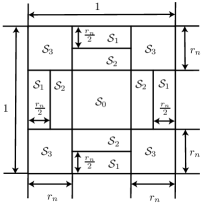
Figure 3: We partition the unit square $\mathcal{S}$ into $\mathcal{S}_{0},\mathcal{S}_{1},\mathcal{S}_{2}$ and $\mathcal{S}_{3}$. Note that each of $\mathcal{S}_{1},\mathcal{S}_{2}$ and $\mathcal{S}_{3}$ has four parts.

B.3.1 Establishing (38) on the unit square $\mathcal{S}$

By Lemma 2, $\mathbb{P}[I_{x}]=\int_{\mathcal{S}}e^{-np_{s}D_{{r_{n}}}(\hat{v_{x}})}\,\textrm{d}\hat{v_{x}}$ holds. To compute $\mathbb{P}[I_{x}]$ based on this, we partition $\mathcal{S}$ in a way similar to that by Li et al. [12] and Wan et al. [20]. Specifically, $\mathcal{S}$ is divided into $\mathcal{S}_{0},\mathcal{S}_{1},\mathcal{S}_{2}$ and $\mathcal{S}_{3}$, respectively, as illustrated in Figure 3 (note that $r_{n}<\frac{1}{2}$ for all $n$ sufficiently large due to $r_{n}=o(1)$ by Lemma 4). $\mathcal{S}_{0}$ consists of all points each with a distance greater than ${r_{n}}$ to its nearest edge of $\mathcal{S}$, whereas $\mathcal{S}_{3}$ is the area in which each point has distances no greater than ${r_{n}}$ to at least two edges of $\mathcal{S}$. We further divide $\mathcal{S}\setminus\{\mathcal{S}_{0}\cup\mathcal{S}_{3}\}$ into $\mathcal{S}_{1}$ and $\mathcal{S}_{2}$ as follows. In $\mathcal{S}\setminus\{\mathcal{S}_{0}\cup\mathcal{S}_{3}\}$, $\mathcal{S}_{1}$ compromise points whose distance to the nearest edge of $\mathcal{S}$ is no greater than $\frac{{r_{n}}}{2}$, while the remaining area is $\mathcal{S}_{2}$; i.e., $\mathcal{S}_{2}=\mathcal{S}\setminus\{\mathcal{S}_{0}\cup\mathcal{S}_{1}\cup\mathcal{S}_{3}\}$.

For $i=0,1,2,3$, we define

$$T_{i}: =\int_{\mathcal{S}_{i}}e^{-np_{s}|D_{{r_{n}}}(\hat{v_{x}})|}\,\textrm{d}\hat{v_{x}}.$$ (49)

Then it is clear that $\mathbb{P}[I_{x}]=\sum_{i=0}^{3}T_{i}$. From (24) in Lemma 4, there exists $\delta_{n}$ with $\delta_{n}=\alpha_{n}\pm O(1)$ such that (i) if $p_{s}=\omega\left(\frac{1}{n^{1/3}\ln n}\right)$, then

$$\pi{r_{n}}^{2}{p_{s}} =\frac{\ln\frac{n}{{p_{s}}}-\ln\ln\frac{n}{{p_{s}}}+\delta_{n}}{n};$$ (50)

and (ii) if $p_{s}=O\left(\frac{1}{n^{1/3}\ln n}\right)$, then

$$\pi{r_{n}}^{2}{p_{s}} =\frac{4\ln\frac{1}{p_{s}}-4\ln\ln\frac{1}{p_{s}}+\delta_{n}}{n}.$$ (51)

We explain below in detail that in case (i), $\lim\limits_{n\to\infty}T_{1}=\infty$ follows, yielding $\lim\limits_{n\to\infty}\mathbb{P}[I_{x}]=\infty$ (i.e., (38)).

To evaluate $T_{1}$, we introduce some notation as follows. For any position $\hat{v_{x}}\in\mathcal{S}_{1}$, we let the distance from $\hat{v_{x}}$ to the nearest edge of the square $\mathcal{S}$ be $g$, where $0\leq g\leq\frac{{r_{n}}}{2}$. For $\hat{v_{x}}\in\mathcal{S}_{1}$, clearly $|D_{{r_{n}}}(\hat{v_{x}})|$ is determined given $g$; and we denote it by $H(g)$. As used before, we have Lagrange’s notation for differentiation; namely, the first and second derivatives of a function $f$ are denoted by $f^{\prime}$ and $f^{\prime\prime}$, respectively. It is easy to derive

$$H(g) =[\pi-\arccos({g}/{{r_{n}}})]{r_{n}}^{2}+g\sqrt{{r_{n}}^{2}-g^{2}},$$ (52)

$$H^{\prime}(g) =2\sqrt{{r_{n}}^{2}-g^{2}},$$ (53)

and

$$H^{\prime\prime}(g) =-2{g}/{\sqrt{{r_{n}}^{2}-g^{2}}}.$$ (54)

Since $\mathcal{S}_{1}$ consists of four rectangles, each of which has length $1-2{r_{n}}$ and width $\frac{{r_{n}}}{2}$, it follows that

$$T_{1} =\int_{\mathcal{S}_{1}}e^{-p_{s}n|D_{{r_{n}}}(\hat{v_{x}})|}\,\textrm{d}\hat{v_{x}}=4(1-2{r_{n}})\int_{0}^{\frac{{r_{n}}}{2}}e^{-p_{s}nH(g)}\,\textrm{d}g.$$ (55)

For simplicity, we write $H(g)$ as $H$. Then

$$e^{-p_{s}nH}\,\textrm{d}g$$

$$=-(p_{s}n)^{-1}(H^{\prime})^{-1}\,\textrm{d}e^{-p_{s}nH}$$

$$=-(p_{s}n)^{-1}\big{\{}\textrm{d}\big{[}(H^{\prime})^{-1}e^{-p_{s}nH}\big{]}-e^{-p_{s}nH}\,\textrm{d}(H^{\prime})^{-1}\big{\}}$$

$$=(p_{s}n)^{-1}\big{\{}\textrm{d}\big{[}-(H^{\prime})^{-1}e^{-p_{s}nH}\big{]}-(H^{\prime})^{-2}H^{\prime\prime}e^{-p_{s}nH}\textrm{d}g\big{\}}.$$ (56)

From (56) and $H^{\prime\prime}\leq 0$,

$$\int_{0}^{\frac{{r_{n}}}{2}}e^{-p_{s}nH(g)}\,\textrm{d}g\geq\frac{e^{-p_{s}nH(0)}}{p_{s}nH^{\prime}(0)}-\frac{e^{-p_{s}nH\left(\frac{{r_{n}}}{2}\right)}}{p_{s}nH^{\prime}\left(\frac{{r_{n}}}{2}\right)}.$$ (57)

From (52) and (53), then $H(0)=\pi{r_{n}}^{2}/2$, $H^{\prime}(0)=2r_{n}$, $H\left(\frac{{r_{n}}}{2}\right)=\big{(}\frac{2}{3}\pi+\frac{\sqrt{3}}{4}\big{)}{r_{n}}^{2}$ and $H^{\prime}\left(\frac{{r_{n}}}{2}\right)=\sqrt{3}r_{n}$. Using these and $\pi{r_{n}}^{2}{p_{s}}n=\Theta(\ln n)$ from Lemma 4 in (57), we derive

$$\int_{0}^{\frac{{r_{n}}}{2}}e^{-p_{s}nH(g)}\,\textrm{d}g \geq\frac{e^{-\pi{r_{n}}^{2}p_{s}n/2}}{2r_{n}p_{s}n}\cdot[1-o(1)],$$

which along with $r_{n}=o(1)$ from Lemma 4 is applied to (55) so that

$$\mathbb{P}[I_{x}]\geq T_{1} \geq 2(r_{n}p_{s}n)^{-1}e^{-\pi{r_{n}}^{2}p_{s}n/2}\cdot[1-o(1)].$$ (58)

From (50), we get

$$e^{-\pi{r_{n}}^{2}p_{s}n} =e^{-\ln\frac{n}{p_{s}}+\ln\ln\frac{n}{p_{s}}-\delta_{n}}=\frac{p_{s}}{n}e^{-\delta_{n}}\ln\frac{n}{p_{s}},$$ (59)

and with $\Delta$ denoting $\pi{r_{n}}^{2}p_{s}n$ (note that $\Delta=\Theta(\ln n)$ from Lemma 4),

$$r_{n} =\pi^{-\frac{1}{2}}{p_{s}}^{-\frac{1}{2}}n^{-\frac{1}{2}}\Delta^{\frac{1}{2}}.$$ (60)

Then using (59) and (60) in (58), it follows that

$$n\mathbb{P}[I_{x}]$$

$$\geq n\cdot 2\pi^{\frac{1}{2}}{p_{s}}^{-\frac{1}{2}}n^{-\frac{1}{2}}\Delta^{-\frac{1}{2}}\cdot p_{s}^{\frac{1}{2}}{n^{-\frac{1}{2}}}e^{-\frac{\delta_{n}}{2}}\bigg{(}\ln\frac{n}{p_{s}}\bigg{)}^{\frac{1}{2}}\cdot[1-o(1)]$$

$$\geq 2\pi^{\frac{1}{2}}\bigg{(}\Delta^{-1}\ln\frac{n}{p_{s}}\bigg{)}^{\frac{1}{2}}e^{-\frac{\delta_{n}}{2}}\cdot[1-o(1)].$$

From $\Delta=\Theta(\ln n)$ and $\ln\frac{n}{p_{s}}=\Theta(\ln n)$ in Lemma 4, with $\lim\limits_{n\to\infty}\alpha_{n}=-\infty$ producing $\lim\limits_{n\to\infty}\delta_{n}=-\infty$, we have

$$\lim_{n\to\infty}\big{\{}n\mathbb{P}[I_{x}]\big{\}}=\infty.$$

With $p_{s}=O\left(\frac{1}{n^{1/3}\ln n}\right)$, by [15, Equation (8.21)], it follows that

$$\lim_{n\to\infty}\big{\{}n\mathbb{P}[I_{x}]\big{\}}=\infty\textrm{ if }\lim_{n\to\infty}\delta_{n}=-\infty.$$

B.3.2 Establishing (39) on the unit square $\mathcal{S}$

Clearly, (41) and (42) still hold. Here we consider the network area $\mathcal{A}$ as the unit square $\mathcal{S}$. For any $\hat{v_{x}}\in\mathcal{S}$ and any $\hat{v_{y}}\in\mathcal{S}$, we have $|D_{r_{n}}(\hat{v_{x}})\hskip 2.0pt{\cap}\hskip 2.0ptD_{r_{n}}(\hat{v_{y}})|\leq\pi{r_{n}}^{2}$, which is applied to (42) so that

$$\mathbb{P}\big{[}\hskip 1.0ptI_{x}\hskip 2.0pt{\cap}\hskip 2.0ptI_{y}\boldsymbol{\mid}(|S_{xy}|=u)\hskip 1.0pt\big{]}$$

$$\leq e^{\pi{r_{n}}^{2}\phi_{u}n}\int_{\mathcal{S}}e^{-np_{s}|D_{{r_{n}}}(\hat{v_{x}})|}\,\textrm{d}\hat{v_{x}}\int_{\mathcal{S}}e^{-np_{s}|D_{{r_{n}}}(\hat{v_{y}})|}\,\textrm{d}\hat{v_{y}}$$

$$=e^{\pi{r_{n}}^{2}\phi_{u}n}\cdot\big{\{}\mathbb{P}[I_{x}]\big{\}}^{2},$$ (61)

where we use the result that $\int_{\mathcal{S}}e^{-np_{s}|D_{{r_{n}}}(\hat{v_{x}})|}\,\textrm{d}\hat{v_{x}}$ and $\int_{\mathcal{S}}e^{-np_{s}|D_{{r_{n}}}(\hat{v_{y}})|}\,\textrm{d}\hat{v_{y}}$ both equal $\mathbb{P}[I_{x}]$ in the last step of (61). Then using (61) in (41), we obtain

$$\mathbb{P}[I_{x}\hskip 2.0pt{\cap}\hskip 2.0ptI_{y}]\leq\big{\{}\mathbb{P}[I_{x}]\big{\}}^{2}\cdot\sum_{u=0}^{K_{n}}\Big{\{}\mathbb{P}[|S_{xy}|=u]e^{\pi{r_{n}}^{2}\phi_{u}n}\Big{\}}.$$ (62)

Since (46) also holds here, we know from (46) and (62) that the proof of (39) on $\mathcal{S}$ is completed once we prove

$$2\pi{r_{n}}^{2}n\cdot\frac{{K_{n}}^{4}}{{P_{n}}^{2}}+\frac{{K_{n}}^{2}}{P_{n}-K_{n}}\cdot e^{\pi{r_{n}}^{2}n\frac{K_{n}}{P_{n}}} =o(1).$$ (63)

Under (8) with $\nu_{n}=o(1)$, we have $\frac{{K_{n}}^{2}}{P_{n}}\leq\frac{{\nu_{n}}^{2}}{\ln n}=o\big{(}\frac{1}{\ln n}\big{)}$, so (2) holds. From Lemma 4, it is always true that $\pi{r_{n}}^{2}n\cdot\frac{{K_{n}}^{2}}{P_{n}}=\Theta(\ln n)$, which along with $\frac{{K_{n}}^{2}}{P_{n}}=o\big{(}\frac{1}{\ln n}\big{)}$ and condition $K_{n}\geq c_{2}\sqrt{\frac{P_{n}\ln n}{n^{c_{3}}}}$ in (8) with $c_{3}>0$ leads to $\pi{r_{n}}^{2}n\cdot\frac{{K_{n}}^{4}}{{P_{n}}^{2}}=o(1)$ and

$$e^{\pi{r_{n}}^{2}n\frac{K_{n}}{P_{n}}}=e^{\pi{r_{n}}^{2}n\frac{{K_{n}}^{2}}{P_{n}}\cdot{K_{n}}^{-1}}\to 1,\textrm{ as }n\to\infty.$$ (64)

Then (63) is proved, completing the proof of (39) on $\mathcal{S}$.

Appendix C ESTABLISHING THE ONE–LAWS

From (8), we have $K_{n}=\Omega\left((\ln n)^{3}\right)$, $\frac{K_{n}}{P_{n}}=O\left(\frac{1}{n\ln n}\right)$ and $\frac{{K_{n}}^{2}}{P_{n}}=O\left(\frac{1}{\ln n}\right)$. Therefore, in view that all conditions of Lemma 11 are satisfied, and considering that connectivity is a monotone increasing graph property, we apply Lemma 11 to obtain for some $p_{n}$ with (37),

$$\mathbb{P}[G_{RKG}(n,K_{n},P_{n})\hskip 2.0pt{\cap}\hskip 2.0ptG_{RGG}(n,r_{n},\mathcal{S})\textrm{ is connected.}]$$

$$\geq\mathbb{P}[G_{ER}(n,p_{n})\hskip 2.0pt{\cap}\hskip 2.0ptG_{RGG}(n,r_{n},\mathcal{S})\textrm{ is connected.}]-o(1).$$ (65)

Here we also define $\nu_{n}$ through (LABEL:lem:erg_rgg_rnpn). We will show that under (8) and (9), $\nu_{n}$ specified in (LABEL:lem:erg_rgg_rnpn) of Lemma 10 equals $\alpha_{n}\pm O(1)$, where $\alpha_{n}$ is set in (9).

In order to assess $\nu_{n}$, we see from (LABEL:lem:erg_rgg_rnpn) that it is useful to evaluate $\ln\frac{1}{p_{n}}$ and $\ln\ln\frac{1}{p_{n}}$. Given (37), we obtain

$$\ln\frac{1}{p_{n}} =\ln\frac{P_{n}}{{K_{n}}^{2}}-\ln\left[1-O\left(\frac{1}{\ln n}\right)\right]$$

$$=\ln\frac{P_{n}}{{K_{n}}^{2}}-O\left(\frac{1}{\ln n}\right),$$ (66)

and with $\frac{{K_{n}}^{2}}{P_{n}}=O\left(\frac{1}{\ln n}\right)$,

$$\ln\ln\frac{1}{p_{n}} =\ln\left[\ln\frac{P_{n}}{{K_{n}}^{2}}-O\left(\frac{1}{\ln n}\right)\right]$$

$$=\ln\left\{\ln\frac{P_{n}}{{K_{n}}^{2}}\left[1-O\left(\frac{1}{\ln n\ln\ln n}\right)\right]\right\}$$

$$=\ln\ln\frac{P_{n}}{{K_{n}}^{2}}-O\left(\frac{1}{\ln n\ln\ln n}\right).$$ (67)

By (37), it holds that

$$p_{n} \sim\frac{{K_{n}}^{2}}{P_{n}},$$

so we have

$$p_{n} =\omega\left(\frac{1}{n^{1/3}\ln n}\right)\textrm{ if and only if }\frac{{K_{n}}^{2}}{P_{n}}=\omega\left(\frac{1}{n^{1/3}\ln n}\right),$$ (68)

and

$$p_{n} =O\left(\frac{1}{n^{1/3}\ln n}\right)\textrm{ if and only if }\frac{{K_{n}}^{2}}{P_{n}}=O\left(\frac{1}{n^{1/3}\ln n}\right).$$ (69)

Now it is ready to compute $\nu_{n}$ according to (LABEL:lem:erg_rgg_rnpn). On the one hand, for $\frac{{K_{n}}^{2}}{P_{n}}=\omega\left(\frac{1}{n^{1/3}\ln n}\right)$ which is equivalent to $p_{n}=\omega\left(\frac{1}{n^{1/3}\ln n}\right)$ in view of (68), we apply (LABEL:lem:erg_rgg_rnpn) (66) and (67) to derive

$$\nu_{n} =\pi{r_{n}}^{2}p_{n}\cdot n-\bigg{(}\ln\frac{n}{p_{n}}-\ln\ln\frac{n}{p_{n}}\bigg{)}$$

$$=\pi{r_{n}}^{2}\cdot\frac{{K_{n}}^{2}}{P_{n}}\cdot\left[1-O\left(\frac{1}{\ln n}\right)\right]\cdot n$$

$$\quad-\bigg{[}\ln\frac{nP_{n}}{{K_{n}}^{2}}-O\left(\frac{1}{\ln n}\right)\bigg{]}$$

$$\quad+\ln\ln\frac{nP_{n}}{{K_{n}}^{2}}-O\left(\frac{1}{\ln n\ln\ln n}\right)$$ (70)

With $\pi{r_{n}}^{2}\cdot\frac{{K_{n}}^{2}}{P_{n}}=\Theta\big{(}\frac{\ln n}{n}\big{)}$,

$$\nu_{n} =\pi{r_{n}}^{2}\cdot\frac{{K_{n}}^{2}}{P_{n}}\cdot n-\ln\frac{nP_{n}}{{K_{n}}^{2}}+\ln\ln\frac{nP_{n}}{{K_{n}}^{2}}$$

$$\quad-\Theta(\ln n)\cdot O\left(\frac{1}{\ln n}\right)+O\left(\frac{1}{\ln n}\right)-O\left(\frac{1}{\ln n\ln\ln n}\right)$$

$$=\alpha_{n}\pm O(1).$$ (71)

On the other hand, for $\frac{{K_{n}}^{2}}{P_{n}}=O\left(\frac{1}{n^{1/3}\ln n}\right)$ that is equivalent to $p_{n}=O\left(\frac{1}{n^{1/3}\ln n}\right)$ in view of (69), we use (LABEL:lem:erg_rgg_rnpn) (66) and (67) to obtain

$$\nu_{n} =\pi{r_{n}}^{2}p_{n}\cdot n-\bigg{(}4\ln\frac{1}{p_{n}}-4\ln\ln\frac{1}{p_{n}}\bigg{)}$$

$$=\pi{r_{n}}^{2}\cdot\frac{{K_{n}}^{2}}{P_{n}}\cdot\left[1-O\left(\frac{1}{\ln n}\right)\right]\cdot n$$

$$\quad-4\bigg{[}\ln\frac{P_{n}}{{K_{n}}^{2}}-O\left(\frac{1}{\ln n}\right)\bigg{]}$$

$$\quad+4\bigg{[}\ln\ln\frac{P_{n}}{{K_{n}}^{2}}-O\left(\frac{1}{\ln n\ln\ln n}\right)\bigg{]}$$ (72)

Then

$$\nu_{n} =\pi{r_{n}}^{2}\cdot\frac{{K_{n}}^{2}}{P_{n}}\cdot n-4\ln\frac{P_{n}}{{K_{n}}^{2}}+4\ln\ln\frac{P_{n}}{{K_{n}}^{2}}$$

$$\quad-\Theta(\ln n)\cdot O\left(\frac{1}{\ln n}\right)+O\left(\frac{1}{\ln n}\right)-O\left(\frac{1}{\ln n\ln\ln n}\right)$$

$$=\alpha_{n}\pm O(1).$$ (73)

Summarizing (71) and (73), with (8) and (9), $\nu_{n}$ defined in (LABEL:lem:erg_rgg_rnpn) equals $\alpha_{n}\pm O(1)$ specified in (9). Then by Lemmas 10 and 11, the result follows.

Appendix D ESTABLISHING THE LEMMAS

D.1 The Proof of Lemma 2

When node $v_{x}$ is at position $\hat{v_{x}}$, the number of nodes within area $D_{r_{n}}(\hat{v_{x}})$ follows a Poisson distribution with mean $nD_{r_{n}}(\hat{v_{x}})$; and to have an edge with $v_{x}$ in graph $G_{\textrm{Poisson}}(n,\theta_{n},\mathcal{A})$, a node not only has to be within a $D_{r_{n}}(\hat{v_{x}})$ but also has to share at least a key with node $v_{x}$. Then by Lemma 1, the number of nodes neighboring to $v_{x}$ at $\hat{v_{x}}$ follows a Poisson distribution with mean $np_{s}|D_{r_{n}}(\hat{v_{x}})|$; and the probability that such number is $0$ equals $e^{-np_{s}|D_{r_{n}}(\hat{v_{x}})|}$. Integrating $\hat{v_{x}}$ over $\mathcal{A}$, we derive the probability that node $v_{x}$ is isolated (i.e., $\mathbb{P}[I_{x}]$) via

$$\mathbb{P}[I_{x}] =n\int_{\mathcal{A}}e^{-np_{s}|D_{r_{n}}(\hat{v_{x}})|}\,\textrm{d}\hat{v_{x}};$$

namely, (21) follows.

Below we demonstrate (22) and (23). For the ease of explanation, we define

$$\mathcal{E}\big{[}(v_{x}\textrm{ at }\hat{v_{x}})\hskip 2.0pt{\cap}\hskip 2.0pt(v_{y}\textrm{ at }\hat{v_{y}})\hskip 2.0pt{\cap}\hskip 2.0pt(|S_{xy}|=u)\big{]}$$

as the event that

• nodes $v_{x}$ and $v_{y}$ are at positions $\hat{v_{x}}$ and $\hat{v_{y}}$, respectively;

• and $v_{x}$ and $v_{y}$ share a certain number $u$ of keys, where $u=0,1,\ldots,K_{n}$.

Conditioning on $\mathcal{E}\big{[}(v_{x}\textrm{ at }\hat{v_{x}})\hskip 2.0pt{\cap}\hskip 2.0pt(v_{y}\textrm{ at }\hat{v_{y}})\hskip 2.0pt{\cap}\hskip 2.0pt(|S_{xy}|=u)\big{]}$, we further define $N(\mathcal{E})$ as the number of nodes different from $v_{x}$ and $v_{y}$, and neighboring to at least one of $v_{x}$ and $v_{y}$. By Lemma 1, $N(\mathcal{E})$ follows a Poisson distribution with mean

$$n\cdot{\mathbb{P}}\bigg{[}\hskip 1.0pt\textrm{E}_{{x}j}\hskip 2.0pt{\cup}\hskip 2.0pt\textrm{E}_{{y}j}\hskip 2.0pt\boldsymbol{\bigg{|}}\hskip 2.0pt{(|S_{xy}|=u)}\begin{array}[]{l}{\small\hskip 2.0pt{\cap}\hskip 2.0pt(v_{x}\textrm{ is at }\hat{v_{x}}),}\\ {\small\hskip 2.0pt{\cap}\hskip 2.0pt(v_{y}\textrm{ is at }\hat{v_{y}}).}\end{array}\bigg{]},$$ (76)

which we denote by $\lambda_{\hat{v_{x}},\hat{v_{y}},u}$ below.

Conditioning on $\mathcal{E}\big{[}(v_{x}\textrm{ at }\hat{v_{x}})\hskip 2.0pt{\cap}\hskip 2.0pt(v_{y}\textrm{ at }\hat{v_{y}})\hskip 2.0pt{\cap}\hskip 2.0pt(|S_{xy}|=u)\big{]}$, event $I_{x}\hskip 2.0pt{\cap}\hskip 2.0ptI_{y}$ (i.e., the event that nodes $v_{x}$ and $v_{y}$ are both isolated) is equivalent to $N(\mathcal{E})\hskip 2.0pt{\cap}\hskip 2.0pt\overline{E_{xy}}$. Conditioning on event $(|S_{xy}|=u)$, for event $\overline{E_{xy}}$ to occur, the distance between $v_{x}$ at $\hat{v_{x}}$ and $v_{y}$ at $\hat{v_{y}}$ has to be greater than distance $r_{n}$ for $u=1,2,\ldots,K_{n}$; and there is no such requirement for $u=0$ as $(|S_{xy}|=0)$ already implies $\overline{E_{xy}}$. Therefore, we obtain

$$\mathbb{P}\Big{[}I_{x}\hskip 2.0pt{\cap}\hskip 2.0ptI_{y}\hskip 2.0pt\boldsymbol{\Big{|}}\hskip 2.0pt\mathcal{E}\big{[}(v_{x}\textrm{ at }\hat{v_{x}})\hskip 2.0pt{\cap}\hskip 2.0pt(v_{y}\textrm{ at }\hat{v_{y}})\hskip 2.0pt{\cap}\hskip 2.0pt(|S_{xy}|=0)\big{]}\Big{]}$$

$$\quad=\mathbb{P}\big{[}N(\mathcal{E})=0\big{]}$$

$$\quad=e^{-n\lambda_{\hat{v_{x}},\hat{v_{y}},0}},$$ (77)

where $\lambda_{\hat{v_{x}},\hat{v_{y}},0}$ stands for $\lambda_{\hat{v_{x}},\hat{v_{y}},u}$ when $u=0$; and for $u=1,2,\ldots,K_{n}$,

• if $\hat{v_{x}}$ and $\hat{v_{y}}$ has a distance greater than $r_{n}$, then

  $$\mathbb{P}\Big{[}I_{x}\hskip 2.0pt{\cap}\hskip 2.0ptI_{y}\hskip 2.0pt\boldsymbol{\Big{|}}\hskip 2.0pt\mathcal{E}\big{[}(v_{x}\textrm{ at }\hat{v_{x}})\hskip 2.0pt{\cap}\hskip 2.0pt(v_{y}\textrm{ at }\hat{v_{y}})\hskip 2.0pt{\cap}\hskip 2.0pt(|S_{xy}|=u)\big{]}\Big{]}$$

  $$\quad=\mathbb{P}\big{[}N(\mathcal{E})=0\big{]}$$

  $$\quad=e^{-n\lambda_{\hat{v_{x}},\hat{v_{y}},u}};$$ (78)

• and if $\hat{v_{x}}$ and $\hat{v_{y}}$ has a distance no greater than distance $r_{n}$, then

  $$\mathbb{P}\Big{[}I_{x}\hskip 2.0pt{\cap}\hskip 2.0ptI_{y}\hskip 2.0pt\boldsymbol{\Big{|}}\hskip 2.0pt\mathcal{E}\big{[}(v_{x}\textrm{ at }\hat{v_{x}})\hskip 2.0pt{\cap}\hskip 2.0pt(v_{y}\textrm{ at }\hat{v_{y}})\hskip 2.0pt{\cap}\hskip 2.0pt(|S_{xy}|=u)\big{]}\Big{]}$$

  $$\quad=0.$$ (79)

For $u=0,1,\ldots,K_{n}$, integrating

$$\mathbb{P}\Big{[}I_{x}\hskip 2.0pt{\cap}\hskip 2.0ptI_{y}\hskip 2.0pt\boldsymbol{\Big{|}}\hskip 2.0pt\mathcal{E}\big{[}(v_{x}\textrm{ at }\hat{v_{x}})\hskip 2.0pt{\cap}\hskip 2.0pt(v_{y}\textrm{ at }\hat{v_{y}})\hskip 2.0pt{\cap}\hskip 2.0pt(|S_{xy}|=u)\big{]}\Big{]}$$

with $\hat{v_{x}}$ over $\mathcal{A}$ and $\hat{v_{y}}$ also over $\mathcal{A}$, we then obtain $\mathbb{P}\big{[}I_{x}\hskip 2.0pt{\cap}\hskip 2.0ptI_{y}\boldsymbol{\mid}(|S_{xy}|=u)\big{]}$. Hence, in view of (77–79), it is easy to establish

$$\mathbb{P}\big{[}I_{x}\hskip 2.0pt{\cap}\hskip 2.0ptI_{y}\boldsymbol{\mid}(|S_{xy}|=u)\big{]}$$

$$~{}=\int_{\mathcal{A}}\int_{\mathcal{A}\setminus D_{r}(\hat{v_{x}})}e^{-n\lambda_{\hat{v_{x}},\hat{v_{y}},u}}\,\textrm{d}\hat{v_{x}}\,\textrm{d}\hat{v_{y}};$$ (80)

and

$$\mathbb{P}\big{[}I_{x}\hskip 2.0pt{\cap}\hskip 2.0ptI_{y}\boldsymbol{\mid}(|S_{xy}|=0)\big{]}$$

$$~{}=\int_{\mathcal{A}}\int_{\mathcal{A}}e^{-n\lambda_{\hat{v_{x}},\hat{v_{y}},0}}\,\textrm{d}\hat{v_{x}}\,\textrm{d}\hat{v_{y}}.$$ (81)

To evaluate (80) and (81), we calculate $\lambda_{\hat{v_{x}},\hat{v_{y}},u}$ below based on its expression in (76). By (76), it is clear that

$$\lambda_{\hat{v_{x}},\hat{v_{y}},u}$$

$$=n\cdot{\mathbb{P}}\bigg{[}\hskip 1.0pt\textrm{E}_{{x}j}\hskip 2.0pt\boldsymbol{\bigg{|}}\hskip 2.0pt{(|S_{xy}|=u)}\begin{array}[]{l}{\small\hskip 2.0pt{\cap}\hskip 2.0pt(v_{x}\textrm{ is at }\hat{v_{x}}),}\\ {\small\hskip 2.0pt{\cap}\hskip 2.0pt(v_{y}\textrm{ is at }\hat{v_{y}}).}\end{array}\bigg{]}$$ (84)

$$\quad+n\cdot{\mathbb{P}}\bigg{[}\hskip 1.0pt\textrm{E}_{{x}j}\hskip 2.0pt\boldsymbol{\bigg{|}}\hskip 2.0pt{(|S_{xy}|=u)}\begin{array}[]{l}{\small\hskip 2.0pt{\cap}\hskip 2.0pt(v_{x}\textrm{ is at }\hat{v_{x}}),}\\ {\small\hskip 2.0pt{\cap}\hskip 2.0pt(v_{y}\textrm{ is at }\hat{v_{y}}).}\end{array}\bigg{]}$$ (87)

$$\quad-n\cdot{\mathbb{P}}\bigg{[}\hskip 1.0pt\textrm{E}_{{x}j}\hskip 2.0pt{\cap}\hskip 2.0pt\textrm{E}_{{y}j}\hskip 2.0pt\boldsymbol{\bigg{|}}\hskip 2.0pt{(|S_{xy}|=u)}\begin{array}[]{l}{\small\hskip 2.0pt{\cap}\hskip 2.0pt(v_{x}\textrm{ is at }\hat{v_{x}}),}\\ {\small\hskip 2.0pt{\cap}\hskip 2.0pt(v_{y}\textrm{ is at }\hat{v_{y}}).}\end{array}\bigg{]}.$$ (90)

To further assess (90), we have the following observations. To begin with,

$$\textrm{E}_{{x}j} =\textrm{K}_{{x}j}\cap\big{[}\hskip 1.0ptv_{j}\textrm{ is within }D_{r}(\hat{v_{x}})\hskip 1.0pt\big{]}.$$ (91)

Each of $K_{{x}j}$ and $K_{{y}j}$ is independent of $(|S_{xy}|=u)$, but $K_{{x}j}\hskip 2.0pt{\cap}\hskip 2.0ptK_{{y}j}$ is not independent of $(|S_{xy}|=u)$. Clearly,

$${\mathbb{P}}\big{[}K_{{x}j}\boldsymbol{\mid}(|S_{xy}|=u)\big{]} ={\mathbb{P}}\big{[}K_{{x}j}\big{]}=p_{s},$$ (92)

and

$${\mathbb{P}}\big{[}K_{{y}j}\boldsymbol{\mid}(|S_{xy}|=u)\big{]} ={\mathbb{P}}\big{[}K_{{y}j}\big{]}=p_{s}.$$ (93)

We also recall

$$\phi_{u}={\mathbb{P}}\big{[}\hskip 1.0ptK_{{x}j}\hskip 2.0pt{\cap}\hskip 2.0ptK_{{y}j}\boldsymbol{\mid}(|S_{xy}|=u)\hskip 1.0pt\big{]}.$$ (94)

Then we use (91–94) in (90) to derive

$$\lambda_{\hat{v_{x}},\hat{v_{y}},u} =np_{s}\cdot{\big{[}}\big{|}D_{r_{n}}(\hat{v_{x}})\big{|}+\big{|}D_{r_{n}}(\hat{v_{y}})\big{|}{\big{]}}$$

$$\quad-n\phi_{u}\cdot\big{|}D_{r_{n}}(\hat{v_{x}})\hskip 2.0pt{\cap}\hskip 2.0ptD_{r_{n}}(\hat{v_{y}})\big{|}.$$ (95)

Substituting (95) into (80) and (81), we establish (22) and (23), respectively. $\square$

D.2 The Proof of Lemma 3

Given (4) and $\alpha_{n}<0$, we obtain ${\pi{r_{n}}^{2}\cdot\frac{{K_{n}}^{2}}{P_{n}}}\cdot n\leq\ln n$, which together with $\frac{{K_{n}}^{2}}{P_{n}}\geq\frac{{\mu_{n}}^{2}\ln n}{n}=\omega\big{(}\frac{\ln n}{n}\big{)}$ resulted from condition (3) brings about $r_{n}=o(1)$ because of $\pi r_{n}^{2}=O\big{(}\frac{\ln n}{n}\big{)}\cdot\big{[}\omega\big{(}\frac{\ln n}{n}\big{)}\big{]}^{-1}=o(1)$. With condition (3), it follows that $\frac{{K_{n}}^{2}}{P_{n}}\leq\frac{{c_{1}}^{2}}{\ln n}=O(\frac{1}{\ln n})$. Then from (2) (4) and ${\pi{r_{n}}^{2}\cdot\frac{{K_{n}}^{2}}{P_{n}}}\cdot n\leq\ln n$, we obtain

$$\pi{r_{n}}^{2}{p_{s}}n =\pi{r_{n}}^{2}\cdot\frac{{K_{n}}^{2}}{P_{n}}\cdot n\cdot\bigg{[}1-O\bigg{(}\frac{{K_{n}}^{2}}{P_{n}}\bigg{)}\bigg{]}$$

$$=\ln n+\alpha_{n}-O(\ln n)\cdot O\bigg{(}\frac{1}{\ln n}\bigg{)}$$

$$=\ln n+\alpha_{n}-O(1).$$

D.3 The Proof of Lemma 4

From $\frac{{c_{2}}^{2}\ln n}{n^{c_{3}}}\leq\frac{{K_{n}}^{2}}{P_{n}}\leq\frac{{\nu_{n}}^{2}}{\ln n}$, (1) and (2), there exists $\varphi_{n}$ with $\lim\limits_{n\to\infty}\varphi_{n}=1$ such that $\frac{{c_{2}}^{2}\ln n}{n^{c_{3}}}\cdot\varphi_{n}\leq p_{s}\leq\frac{{\nu_{n}}^{2}}{\ln n}$. Then $\ln(n/p_{s})\leq(1+c_{3})\ln n-\ln\ln n-\ln\varphi_{n}-2\ln c_{2}$ and $\ln(n/p_{s})\geq\ln n+\ln\ln n-2\ln\nu_{n}$ hold, leading to $\ln(n/p_{s})=\Theta(\ln n)$. Similarly, $\ln\frac{nP_{n}}{{K_{n}}^{2}}=\Theta(\ln n)$. For $\frac{{K_{n}}^{2}}{P_{n}}=O\left(\frac{1}{n^{1/3}\ln n}\right)$, then in view of $\ln\frac{nP_{n}}{{K_{n}}^{2}}=\Theta(\ln n)$, $\pi{r_{n}}^{2}\cdot\frac{{K_{n}}^{2}}{P_{n}}\cdot n=\ln\frac{nP_{n}}{{K_{n}}^{2}}-\ln\ln\frac{nP_{n}}{{K_{n}}^{2}}+\alpha_{n}$ resulted from (9), and $|\alpha_{n}|=O(\ln\ln n)$, we obtain $\pi{r_{n}}^{2}\cdot\frac{{K_{n}}^{2}}{P_{n}}=\Theta\big{(}\frac{\ln n}{n}\big{)}$. On the other hand, for $\frac{{K_{n}}^{2}}{P_{n}}=\omega\left(\frac{1}{n^{1/3}\ln n}\right)$, then we apply $\ln\frac{P_{n}}{{K_{n}}^{2}}=\ln\left[\omega\left(n^{1/3}\ln n\right)\right]=\Theta(\ln n)$ and condition $\pi{r_{n}}^{2}\cdot\frac{{K_{n}}^{2}}{P_{n}}\cdot n4\ln\frac{P_{n}}{{K_{n}}^{2}}-4\ln\ln\frac{P_{n}}{{K_{n}}^{2}}+\alpha_{n}$ from (9) and $|\alpha_{n}|=O(\ln\ln n)$ to derive $\pi{r_{n}}^{2}\cdot\frac{{K_{n}}^{2}}{P_{n}}=\Theta\big{(}\frac{\ln n}{n}\big{)}$. Hence, under either $\frac{{K_{n}}^{2}}{P_{n}}=O\left(\frac{1}{n^{1/3}\ln n}\right)$ or $\frac{{K_{n}}^{2}}{P_{n}}=\omega\left(\frac{1}{n^{1/3}\ln n}\right)$, it holds that $\pi{r_{n}}^{2}\cdot\frac{{K_{n}}^{2}}{P_{n}}=\Theta\big{(}\frac{\ln n}{n}\big{)}$, which along with (2) and $\frac{{K_{n}}^{2}}{P_{n}}\geq\frac{{c_{2}}^{2}\ln n}{n^{c_{3}}}$ resulting in $\pi{r_{n}}^{2}\cdot p_{s}=\Theta\big{(}\frac{\ln n}{n}\big{)}$ and $r_{n}=o(1)$, respectively.

In order to assess $\delta_{n}$, we see from (24) that it is useful to evaluate $\ln\frac{1}{p_{s}}$ and $\ln\ln\frac{1}{p_{s}}$. From $\frac{{K_{n}}^{2}}{P_{n}}\leq\frac{{\nu_{n}}^{2}}{\ln n}$ and (2), then we obtain $\ln\frac{1}{p_{s}}=\ln\frac{P_{n}}{{K_{n}}^{2}}-O\left(\frac{1}{\ln n}\right)$, which leads to
$\ln\ln\frac{1}{p_{s}}=\ln\big{[}\ln\frac{P_{n}}{{K_{n}}^{2}}-O\left(\frac{1}{\ln n}\right)\big{]}=\ln\ln\frac{P_{n}}{{K_{n}}^{2}}-O\left(\frac{1}{\ln n\ln\ln n}\right)$.

Now it is ready to compute $\delta_{n}$. In view of (2), clearly $p_{s}=O\left(\frac{1}{n^{1/3}\ln n}\right)$ (resp., $p_{s}=\omega\left(\frac{1}{n^{1/3}\ln n}\right)$) is equivalent to $p_{s}=\omega\left(\frac{1}{n^{1/3}\ln n}\right)$ (resp., $\frac{{K_{n}}^{2}}{P_{n}}=\omega\left(\frac{1}{n^{1/3}\ln n}\right)$). We apply the expressions of $\ln\frac{1}{p_{s}}$ and $\ln\ln\frac{1}{p_{s}}$ above, $\pi{r_{n}}^{2}\cdot\frac{{K_{n}}^{2}}{P_{n}}\cdot n=\Theta(\ln n)$, (9) and (24) to show that under either $p_{s}=O\left(\frac{1}{n^{1/3}\ln n}\right)$ or $p_{s}=\omega\left(\frac{1}{n^{1/3}\ln n}\right)$, we always have

$$\delta_{n} =\alpha_{n}-\Theta(\ln n)\cdot O\left(\frac{1}{\ln n}\right)+O\left(\frac{1}{\ln n}\right)-O\left(\frac{1}{\ln n\ln\ln n}\right)\vspace{-5pt}$$

$$=\alpha_{n}\pm O(1).$$

D.4 The Proof of Lemma 5

To begin with, it holds that

$$\mathbb{P}[K_{{xz}}\cap K_{yz}\boldsymbol{\mid}(|S_{xy}|=u)]$$

$$~{}=\mathbb{P}[K_{{xz}}\boldsymbol{\mid}(|S_{xy}|=u)]+\mathbb{P}[K_{yz}\boldsymbol{\mid}(|S_{xy}|=u)]$$

$$~{}\quad-(1-\mathbb{P}[\overline{K_{{xz}}}\cap\overline{K_{yz}}\boldsymbol{\mid}(|S_{xy}|=u)])$$

$$~{}=2p_{s}-1+\binom{P_{n}-(2K_{n}-u)}{K_{n}}\bigg{/}\binom{P_{n}}{K_{n}}.\vspace{-5pt}$$ (96)

By [22, Lemma 7.1] and [24, Fact 2], it follows that

$$\binom{P_{n}-(2K_{n}-u)}{K_{n}}\bigg{/}\binom{P_{n}}{K_{n}}\leq\bigg{(}1-\frac{2K_{n}-u}{P_{n}}\bigg{)}^{K_{n}}$$

$$\leq 1-\frac{(2K_{n}-u)K_{n}}{P_{n}}\cdot{K_{n}}+\frac{1}{2}\bigg{[}\frac{(2K_{n}-u)K_{n}}{P_{n}}\bigg{]}^{2}.\vspace{-5pt}$$ (97)

Applying (1) (i.e., $p_{s}\leq\frac{{K_{n}}^{2}}{P_{n}}$) and (97) to (96), we have

$$\mathbb{P}[({K}_{xz}\cap{K}_{yz}\boldsymbol{\mid}(|S_{xy}|=u)] \leq\frac{u{K_{n}}}{P_{n}}+\frac{2{K_{n}}^{4}}{{P_{n}}^{2}}.$$

D.5 The Proof of Lemma 6

From (40), it follows that

$$n\mathbb{P}[I_{x}] =ne^{-\pi{r_{n}}^{2}p_{s}n}=ne^{-\ln n-\alpha_{n}\pm O(1)}.$$

With $|\alpha_{n}|=O(\ln\ln n)$, we have for any constant $\epsilon>0$,

$$n\mathbb{P}[I_{x}]=o(n^{\epsilon}).$$

D.6 The Proof of Lemma 7

As in Section B.3.1, we partition $\mathcal{S}$ according to Figure 3 and define $T_{i}$ for $i=0,1,2,3$ according to (49); i.e.,

$$T_{i}: =\int_{\mathcal{S}_{i}}e^{-np_{s}|D_{{r_{n}}}(\hat{v_{x}})|}\,\textrm{d}\hat{v_{x}}.$$

Then

$$\mathbb{P}[I_{x}] =\sum_{i=0}^{3}T_{i}.$$ (98)

To compute $T_{0}$, we use $D_{{r_{n}}}(\hat{v_{x}})=\pi{r_{n}}^{2}$ for any position $\hat{v_{x}}\in\mathcal{S}_{0}$, and $|\mathcal{S}_{0}|=(1-2{r_{n}})^{2}\leq 1$ to derive

$$T_{0} =\int_{\mathcal{S}_{0}}e^{-p_{s}n|D_{{r_{n}}}(\hat{v_{x}})|}\,\textrm{d}\hat{v_{x}}\leq e^{-\pi{r_{n}}^{2}p_{s}n}.$$ (99)

We present below an upper bound on $T_{1}$. In view of (56), we further have

$$-(H^{\prime})^{-2}H^{\prime\prime}e^{-p_{s}nH}\,\textrm{d}g$$

$$\quad=-(H^{\prime})^{-3}H^{\prime\prime}e^{-p_{s}nH}\,\textrm{d}H$$

$$\quad=-(p_{s}n)^{-1}(H^{\prime})^{-3}H^{\prime\prime}\,\textrm{d}\big{(}-e^{-p_{s}nH}\big{)}.$$ (100)

For $0\leq g\leq\frac{{r_{n}}}{2}$, it holds from (53) and (54) that

$$-\frac{H^{\prime\prime}}{(H^{\prime})^{3}} =\frac{g}{4({r_{n}}^{2}-g^{2})^{2}}\leq\frac{\frac{{r_{n}}}{2}}{4\times\left(\frac{3}{4}{r_{n}}^{2}\right)^{2}}=\frac{2}{9{r_{n}}^{3}}.$$ (101)

By (100) and (101), it follows that

$$-\int_{0}^{\frac{{r_{n}}}{2}}(H^{\prime})^{-2}H^{\prime\prime}e^{-p_{s}nH}\textrm{d}g \leq\frac{2}{9{r_{n}}^{3}p_{s}n}\int_{0}^{\frac{{r_{n}}}{2}}\textrm{d}\big{(}-e^{-p_{s}nH}\big{)}.$$ (102)

Applying (102) to (56),

$$\int_{0}^{\frac{{r_{n}}}{2}}e^{-p_{s}nH(g)}\,\textrm{d}g\leq\frac{e^{-p_{s}nH(0)}}{p_{s}nH^{\prime}(0)}+\frac{2e^{-p_{s}nH(0)}}{9{r_{n}}^{3}{p_{s}}^{2}n^{2}}.$$ (103)

Using (103) in (55),

$$T_{1} \leq\frac{4e^{-p_{s}nH(0)}}{p_{s}nH^{\prime}(0)}+\frac{8e^{-p_{s}nH(0)}}{9{r_{n}}^{3}{p_{s}}^{2}n^{2}}.$$ (104)

From (52) and (53), then $H(0)=\pi{r_{n}}^{2}/2$ and’ $H^{\prime}(0)=2r_{n}$. Using these and $\pi{r_{n}}^{2}{p_{s}}n=\Theta(\ln n)$ from Lemma 4 in (104), we derive

$$T_{1} \leq 2(r_{n}p_{s}n)^{-1}e^{-\pi{r_{n}}^{2}p_{s}n/2}\cdot[1+o(1)].$$ (105)

Now we assess $T_{2}$. For $\hat{v_{x}}\in\mathcal{S}_{2}$, when the distance from $\hat{v_{x}}$ to the nearest edge of $\mathcal{S}$ equals $\frac{{r_{n}}}{2}$, the area $|D_{{r_{n}}}(\hat{v_{x}})|$ reaches its minimum $c_{0}\pi{r_{n}}^{2}$, where $c_{0}:=\frac{2}{3}+\frac{\sqrt{3}}{4\pi}$. Then with $|\mathcal{S}_{2}|=2{r_{n}}(1-2{r_{n}})\leq 2{r_{n}}$, it follows

$$T_{2} =\int_{\mathcal{S}_{2}}e^{-p_{s}n|D_{{r_{n}}}(\hat{v_{x}})|}\,\textrm{d}\hat{v_{x}}\leq 2{r_{n}}e^{-c_{0}\pi{r_{n}}^{2}p_{s}n}.$$ (106)

To evaluate $T_{3}$, we apply ${\pi{r_{n}}^{2}}/{4}\leq D_{{r_{n}}}(\hat{v_{x}})\leq\pi{r_{n}}^{2}$ for any $\hat{v_{x}}\in\mathcal{S}_{3}$, and $|\mathcal{S}_{3}|=4{r_{n}}^{2}$ to obtain

$$T_{3} =\int_{\mathcal{S}_{3}}e^{-p_{s}n|D_{{r_{n}}}(\hat{v_{x}})|}\,\textrm{d}\hat{v_{x}}\leq 4{r_{n}}^{2}e^{-\pi{r_{n}}^{2}p_{s}n/4}.$$ (107)

Substituting (99) (105) (106) and (107) into (98), we derive

$$\mathbb{P}[I_{x}] \leq e^{-\pi{r_{n}}^{2}p_{s}n}+2(r_{n}p_{s}n)^{-1}e^{-\pi{r_{n}}^{2}p_{s}n/2}\cdot[1+o(1)]$$

$$\quad+2{r_{n}}e^{-c_{0}\pi{r_{n}}^{2}p_{s}n}+4{r_{n}}^{2}e^{-\pi{r_{n}}^{2}p_{s}n/4}.$$ (108)

We discuss the following cases (i) and (ii), in which either $\frac{{K_{n}}^{2}}{P_{n}}=\omega\left(\frac{1}{n^{1/3}\ln n}\right)$ or $\frac{{K_{n}}^{2}}{P_{n}}=O\left(\frac{1}{n^{1/3}\ln n}\right)$ holds. We also let $\Delta$ denote $\pi{r_{n}}^{2}p_{s}n$.

(i) We consider $\frac{{K_{n}}^{2}}{P_{n}}=\omega\left(\frac{1}{n^{1/3}\ln n}\right)$, which also yields $p_{s}=\omega\left(\frac{1}{n^{1/3}\ln n}\right)$ by (2). Using (59) and (60) in (108), we obtain

$$n\mathbb{P}[I_{x}] \leq p_{s}e^{-\delta_{n}}\ln\frac{n}{p_{s}}$$

$$\quad+2\pi^{\frac{1}{2}}\Delta^{-\frac{1}{2}}\bigg{(}\ln\frac{n}{p_{s}}\bigg{)}^{\frac{1}{2}}e^{-\frac{\delta_{n}}{2}}\cdot[1+o(1)]$$

$$\quad+2\pi^{-\frac{1}{2}}{p_{s}}^{c_{0}-\frac{1}{2}}n^{\frac{1}{2}-c_{0}}\Delta^{\frac{1}{2}}\bigg{(}\ln\frac{n}{p_{s}}\bigg{)}^{c_{0}}e^{-c_{0}\delta_{n}}$$

$$\quad+4\pi^{-1}{p_{s}}^{-\frac{3}{4}}n^{-\frac{1}{4}}\Delta e^{-\frac{\delta_{n}}{4}}\bigg{(}\ln\frac{n}{p_{s}}\bigg{)}^{\frac{1}{4}}.$$

From $p_{s}=\omega\left(\frac{1}{n^{1/3}\ln n}\right)$, $\Delta=\Theta(\ln n)$ and $\ln\frac{n}{p_{s}}=\Theta(\ln n)$ by Lemma 4, with $|\alpha_{n}|=O(\ln\ln n)$ producing $|\delta_{n}|=O(\ln\ln n)$, we have

$$n\mathbb{P}[I_{x}]=o(n^{\epsilon})\textrm{ for any constant }\epsilon>0.$$

(ii) We consider $\frac{{K_{n}}^{2}}{P_{n}}=O\left(\frac{1}{n^{1/3}\ln n}\right)$, which also yields $p_{s}=O\left(\frac{1}{n^{1/3}\ln n}\right)$ by (2). We obtain

$$r_{n} =\pi^{-\frac{1}{2}}{p_{s}}^{-\frac{1}{2}}n^{-\frac{1}{2}}\Delta^{\frac{1}{2}},$$ (109)

and from (51),

$$e^{-\pi{r_{n}}^{2}p_{s}n} =e^{-4\ln\frac{1}{p_{s}}+4\ln\ln\frac{1}{p_{s}}-\delta_{n}}={p_{s}}^{4}\bigg{(}\ln\frac{1}{p_{s}}\bigg{)}^{4}e^{-\delta_{n}}.$$ (110)

Applying (109) and (110) to (108), we derive

$$n\mathbb{P}[I_{x}] \leq{p_{s}}^{4}\bigg{(}\ln\frac{1}{p_{s}}\bigg{)}^{4}e^{-\delta_{n}}$$

$$\quad+2\pi^{\frac{1}{2}}{p_{s}}^{\frac{3}{2}}n^{\frac{1}{2}}\Delta^{-\frac{1}{2}}\bigg{(}\ln\frac{n}{p_{s}}\bigg{)}^{2}e^{-\frac{\delta_{n}}{2}}$$

$$\quad+2\pi^{-\frac{1}{2}}{p_{s}}^{4c_{0}-\frac{1}{2}}n^{\frac{1}{2}}\Delta^{\frac{1}{2}}\bigg{(}\ln\frac{1}{p_{s}}\bigg{)}^{4c_{0}}e^{-c_{0}\delta_{n}}$$

$$\quad+4\pi^{-1}\Delta e^{-\frac{\delta_{n}}{4}}\ln\frac{1}{p_{s}}.$$

From $\Delta=\Theta(\ln n)$ and $\ln\frac{1}{p_{s}}=\Theta(\ln n)$, $p_{s}=O\left(\frac{1}{n^{1/3}\ln n}\right)$ and $\frac{1}{3}(4c_{0}-\frac{1}{2})>\frac{1}{2}$, with $|\alpha_{n}|=O(\ln\ln n)$ producing $|\delta_{n}|=O(\ln\ln n)$, we have

$$n\mathbb{P}[I_{x}]=o(n^{\epsilon})\textrm{ for any constant }\epsilon>0.$$

D.7 The Proof of Lemma 8

We will establish Lemma 8 using the standard de-Poissonization technique [14, 13, 21]. Let $M$ be the number of nodes in graph $G_{\textrm{Poisson}}(m,\theta_{n},\mathcal{A})$. Clearly, $M$ follows a Poisson distribution with mean $m$. From Chebyshev’s inequality, for any positive $t$,

$$\mathbb{P}[|M-m|\geq t\sqrt{m}] \leq t^{-2}.$$ (111)

Without loss of generosity, we regard $n-n^{\frac{1}{2}+c_{0}}$ as an integer. With $t:=\frac{n-m}{\sqrt{m}}$, substituting $m=n-n^{\frac{1}{2}+c_{0}}$ into (111),

$$\mathbb{P}\big{[}M\leq n-2n^{\frac{1}{2}+c_{0}}\textrm{ or }M\geq n\big{]}\leq\frac{n-n^{\frac{1}{2}+c_{0}}}{n^{1+2c_{0}}}=o(1).$$ (112)

Hence, $n-2n^{\frac{1}{2}+c_{0}}<M<n$ holds almost surely.

When $M<n$, we construct a coupling $\mathcal{C}$ between graphs $G(n,\theta_{n},\mathcal{A})$ and $G_{\textrm{Poisson}}(m,\theta_{n},\mathcal{A})$, by letting the former be the result of adding to the latter graph $(n-M)$ nodes uniformly distributed on $\mathcal{A}$. Then $\mathcal{V}_{P}$ denoting the node set of $G_{\textrm{Poisson}}(m,\theta_{n},\mathcal{A})$ is a subset of $\mathcal{V}$ being the node set of $G(n,\theta_{n},\mathcal{A})$. In addition, it is straightforward to see that the edge set of $G_{\textrm{Poisson}}(m,\theta_{n},\mathcal{A})$ is also a subset of that of $G(n,\theta_{n},\mathcal{A})$. Then under coupling $\mathcal{C}$, graph $G_{\textrm{Poisson}}(m,\theta_{n},\mathcal{A})$ is a subgraph of $G(n,\theta_{n},\mathcal{A})$.

We denote by $D_{X}$ (resp., $D_{P}$) the set of isolated nodes in $G(n,\theta_{n},\mathcal{A})$ (resp., $G_{\textrm{Poisson}}(m,\theta_{n},\mathcal{A})$). To establish Lemma 8, we prove

$$|\mathbb{P}[D_{X}\neq\emptyset]-\mathbb{P}[D_{P}\neq\emptyset]| =o(1),$$

which follows once we demonstrate $\mathbb{P}[D_{X}\neq D_{P}]=o(1)$ in view of

$$\big{|}\mathbb{P}[D_{X}\neq\emptyset]-\mathbb{P}[D_{P}\neq\emptyset]\big{|}$$

$$=\big{|}\mathbb{P}[(D_{X}\neq\emptyset)\hskip 2.0pt{\cap}\hskip 2.0pt(D_{P}=\emptyset)]-\mathbb{P}[(D_{P}\neq\emptyset)\hskip 2.0pt{\cap}\hskip 2.0pt(D_{X}=\emptyset)]\big{|}$$

$$\leq\mathbb{P}[D_{X}\neq D_{P}].$$

It is straightforward to see

$$\mathbb{P}[D_{X}\neq D_{P}]$$

$$\leq\mathbb{P}\big{[}(D_{P}\setminus D_{X}\neq\emptyset)\hskip 2.0pt{\cap}\hskip 2.0pt(n-2n^{\frac{1}{2}+c_{0}}<M<n)\big{]}$$

$$\quad+\mathbb{P}\big{[}(D_{X}\setminus D_{P}\neq\emptyset)\hskip 2.0pt{\cap}\hskip 2.0pt(n-2n^{\frac{1}{2}+c_{0}}<M<n)\big{]}$$

$$\quad+\mathbb{P}\big{[}M\leq n-2n^{\frac{1}{2}+c_{0}}\textrm{ or }M\geq n\big{]},$$

then given (112), we will prove $\mathbb{P}[D_{X}\neq D_{P}]=o(1)$ and thus establish Lemma 8 once showing

$$\mathbb{P}\big{[}(D_{P}\setminus D_{X}\neq\emptyset)\hskip 2.0pt{\cap}\hskip 2.0pt(n-2n^{\frac{1}{2}+c_{0}}<M<n)\big{]} =o(1),$$ (113)

and

$$\mathbb{P}\big{[}(D_{X}\setminus D_{P}\neq\emptyset)\hskip 2.0pt{\cap}\hskip 2.0pt(n-2n^{\frac{1}{2}+c_{0}}<M<n)\big{]} =o(1).$$ (114)

In proving (113) and (114), with $n-2n^{\frac{1}{2}+c_{0}}<M<n$, we consider the coupling $\mathcal{C}$ under which $G_{\textrm{Poisson}}(m,\theta_{n},\mathcal{A})$ is a subgraph of $G(n,\theta_{n},\mathcal{A})$.

D.7.1 The Proof of (113)

Event ($D_{P}\setminus D_{X}\neq\emptyset$) happens if and only if there exists at least one node $v_{i}$ such that $v_{i}\in D_{P}$ and $v_{i}\notin D_{X}$; i.e., $v_{i}$ is isolated in $G_{\textrm{Poisson}}(m,\theta_{n},\mathcal{A})$ but is not isolated in $G(n,\theta_{n},\mathcal{A})$ since $v_{i}\in\mathcal{V}$ by $v_{i}\in D_{P}$. Then there exists at least one node $v^{\prime}$ in $\mathcal{V}_{\overline{P}}:=\mathcal{V}\setminus\mathcal{V}_{P}$ such that $v^{\prime}$ and $v_{i}$ are neighbors in $G(n,\theta_{n},\mathcal{A})$. Due to $\mathcal{V}_{\overline{P}}=n-M<2n^{\frac{1}{2}+c_{0}}$, considering that $p_{e}$ is the edge probability in $G(n,\theta_{n},\mathcal{A})$, then with $L$ denoting the number of isolated nodes in $G_{\textrm{Poisson}}(m,\theta_{n},\mathcal{A})$, it follows via a union bound that

$$\mathbb{P}\big{[}\big{(}D_{P}\setminus D_{X}\neq\emptyset\big{)}\hskip 2.0pt{\cap}\hskip 2.0pt\big{(}n-2n^{\frac{1}{2}+c_{0}}<M<n\big{)}\big{]}$$

$$\quad\leq L\cdot 2n^{\frac{1}{2}+c_{0}}\cdot p_{e}.$$ (115)

For $\mathcal{A}=\mathcal{T}$, we will prove that under conditions (3) and (4) with $|\alpha_{n}|=O(\ln\ln n)$; i.e., with some $\mu_{n}=\omega(1)$ and constant $c_{1}$,

$$\max\bigg{\{}\frac{\ln n}{\ln\ln n},\hskip 1.5pt\mu_{n}\cdot\sqrt{\frac{P_{n}\ln n}{n}}\bigg{\}} \leq K_{n}\leq c_{1}\sqrt{\frac{P_{n}}{\ln n}},$$

for all $n$ sufficiently large, and

$$\pi{r_{n}}^{2}\cdot\frac{{K_{n}}^{2}}{P_{n}} =\frac{\ln n+\alpha_{n}}{n},$$

then there exist some $\widetilde{\mu}_{n}=\omega(1)$ and constant $\widetilde{c}_{1}$ such that

$$\max\bigg{\{}\frac{\ln m}{\ln\ln m},\sqrt{\frac{P_{n}\ln m}{m}}\cdot\widetilde{\mu}_{n}\bigg{\}} \leq K_{n}\leq\widetilde{c}_{1}\sqrt{\frac{P_{n}}{\ln m}}$$ (116)

for all $m$ sufficiently large (i.e., for all $n$ sufficiently large) and

$$\pi{r_{n}}^{2}\cdot\frac{{K_{n}}^{2}}{P_{n}} =\frac{\ln m+\alpha_{n}\pm o(1)}{m},$$ (117)

in order to apply Lemma 6 to $G_{\textrm{Poisson}}(m,\theta_{n},\mathcal{T})$.

We establish (116) as follows. First, with $m<n$, it follows that $\frac{\ln m}{\ln\ln m}<\frac{\ln n}{\ln\ln n}$ for all $n$ sufficiently large since function $f(x)=\frac{\ln x}{\ln\ln x}$ is monotone increasing with $x$ for $x>e^{e}$ by $f^{\prime}(x)=\frac{\ln\ln x-1}{x(\ln\ln x)^{2}}>0$. Thus, under $K_{n}\geq\frac{\ln n}{\ln\ln n}$, it holds that $K_{n}\geq\frac{\ln m}{\ln\ln m}$. Second, with $m=n-n^{\frac{1}{2}+c_{0}}$ and $0<c_{0}<\frac{1}{2}$, then $\frac{\ln m}{m}\sim\frac{\ln n}{n}$, which along with $K_{n}\geq\sqrt{\frac{P_{n}\ln n}{n}}\cdot\mu_{n}$ and $\mu_{n}=\omega(1)$ leads to that there exists some $\widetilde{\mu}_{n}=\omega(1)$ such that $K_{n}\geq\sqrt{\frac{P_{n}\ln m}{m}}\cdot\widetilde{\mu}_{n}$. Third, with $m\sim n$, for all $n$ sufficiently large, we obtain from $K_{n}\leq c_{1}\sqrt{\frac{P_{n}}{\ln n}}$ that $K_{n}\leq\widetilde{c}_{1}\sqrt{\frac{P_{n}}{\ln m}}$. Summarizing the three points above, (116) holds for all $m$ sufficiently large.

We demonstrate (117) in view of

$$m\cdot\pi{r_{n}}^{2}\cdot\frac{{K_{n}}^{2}}{P_{n}}-(\ln m+\alpha_{n})$$

$$=m\cdot\frac{\ln n+\alpha_{n}}{n}-(\ln m+\alpha_{n})$$

$$=\big{(}1-n^{c_{0}-\frac{1}{2}}\big{)}(\ln n+\alpha_{n})-\ln n-\ln\big{(}1-n^{c_{0}-\frac{1}{2}}\big{)}-\alpha_{n}$$

$$=\pm o(1).$$

Then with (116) and (117), we use Lemma 6 to derive

$$L=o(m^{\epsilon})\textrm{ for any constant }\epsilon>0.$$ (118)

For $\mathcal{A}=\mathcal{S}$, we will prove that under conditions (8) and (9) with $|\alpha_{n}|=O(\ln\ln n)$; i.e., with constants $c_{2}>0,$ $0<c_{3}<1$, $c_{4}>0$ and $\nu_{n}=o(1)$,

$$c_{2}\sqrt{\frac{P_{n}\ln n}{n^{c_{3}}}} \leq K_{n}\leq\min\Bigg{\{}\nu_{n}\cdot\sqrt{\frac{P_{n}}{\ln n}},\hskip 1.5pt{\frac{c_{4}P_{n}}{n\ln n}}\hskip 2.0pt\Bigg{\}}$$

for all $n$ sufficiently large, the condition that $\frac{{K_{n}}^{2}}{P_{n}}\cdot n^{1/3}\ln n$ either is bounded for all $n$ or converges to $\infty$ as $n\to\infty$, and

$$\pi{r_{n}}^{2}\cdot\textrm{ $\frac{{K_{n}}^{2}}{P_{n}}$}$$

$$=\begin{cases}\textrm{ $\frac{\ln\frac{nP_{n}}{{K_{n}}^{2}}\hskip 2.0pt-\hskip 2.0pt\ln\ln\frac{nP_{n}}{{K_{n}}^{2}}\hskip 2.0pt+\hskip 2.0pt\alpha_{n}}{n}$},&\textrm{for~{}}\textrm{\large$\frac{{K_{n}}^{2}}{P_{n}}$}=\omega\textrm{\large$\left(\frac{1}{n^{1/3}\ln n}\right)$},\\ \vspace{-7pt}\\ \textrm{ $\frac{4\ln\frac{P_{n}}{{K_{n}}^{2}}\hskip 2.0pt-\hskip 2.0pt4\ln\ln\frac{P_{n}}{{K_{n}}^{2}}\hskip 2.0pt+\hskip 2.0pt\alpha_{n}}{n}$},&\textrm{for~{}}\textrm{\large$\frac{{K_{n}}^{2}}{P_{n}}$}=O\textrm{\large$\left(\frac{1}{n^{1/3}\ln n}\right)$};\end{cases}$$

then there exist some constants $\widetilde{c}_{2}>0$, $0<\widetilde{c}_{3}<1$, $\widetilde{c}_{4}>0$ and $\widetilde{\nu}_{n}=o(1)$, such that

$$\widetilde{c}_{2}\sqrt{\frac{P_{n}\ln m}{m^{\widetilde{c}_{3}}}} \leq K_{n}\leq\min\Bigg{\{}\widetilde{\nu}_{n}\cdot\sqrt{\frac{P_{n}}{\ln m}},\hskip 1.5pt{\frac{\widetilde{c}_{4}P_{n}}{m\ln m}}\hskip 2.0pt\Bigg{\}}$$ (119)

for all $m$ sufficiently large (i.e., for all $n$ sufficiently large); and $\frac{{K_{n}}^{2}}{P_{n}}\cdot m^{1/3}\ln m$ either is bounded for all $m$ or converges to $\infty$ as $m\to\infty$ (i.e., as $n\to\infty$); and $\widetilde{\alpha}_{n}=\alpha_{n}\pm O(1)$ with sequence $\widetilde{\alpha}_{n}$ for all $n$ defined through

$$\pi{r_{n}}^{2}\cdot\frac{{K_{n}}^{2}}{P_{n}}$$

$$=\begin{cases}\textrm{ $\frac{\ln\frac{mP_{n}}{{K_{n}}^{2}}\hskip 2.0pt-\hskip 2.0pt\ln\ln\frac{mP_{n}}{{K_{n}}^{2}}\hskip 2.0pt+\hskip 2.0pt\widetilde{\alpha}_{n}}{m}$},\textrm{~{}for~{}}\textrm{\large$\frac{{K_{n}}^{2}}{P_{n}}$}=\omega\textrm{\large$\left(\frac{1}{m^{1/3}\ln m}\right)$},\\ \vspace{-7pt}\\ \textrm{ $\frac{4\ln\frac{P_{n}}{{K_{n}}^{2}}\hskip 2.0pt-\hskip 2.0pt4\ln\ln\frac{P_{n}}{{K_{n}}^{2}}\hskip 2.0pt+\hskip 2.0pt\widetilde{\alpha}_{n}}{m}$},\textrm{~{}for~{}}\textrm{\large$\frac{{K_{n}}^{2}}{P_{n}}$}=O\textrm{\large$\left(\frac{1}{m^{1/3}\ln m}\right)$},\end{cases}$$ (120)

in order to apply Lemma 7 to $G_{\textrm{Poisson}}(m,\theta_{n},\mathcal{S})$.

We establish (119) as follows. First, due to $K_{n}\geq c_{2}\sqrt{\frac{P_{n}\ln n}{n^{c_{3}}}}$ and $\frac{\ln m}{m^{c_{3}}}\sim\frac{\ln n}{n^{c_{3}}}$, then with $\widetilde{c}_{3}=c_{3}$, there exits some $\widetilde{c}_{2}>0$ such that $K_{n}\geq\widetilde{c}_{2}\sqrt{\frac{P_{n}\ln m}{m^{\widetilde{c}_{3}}}}$. Second, from $\ln m\sim\ln n$ and $K_{n}\leq\nu_{n}\cdot\sqrt{\frac{P_{n}}{\ln n}}$, there exists some $\widetilde{\nu}_{n}=o(1)$ such that $K_{n}\leq\widetilde{\nu}_{n}\cdot\sqrt{\frac{P_{n}}{\ln m}}$. Third, from $m\ln m\sim n\ln n$ and $K_{n}\leq\frac{{c}_{4}P_{n}}{n\ln n}$, there exists some $\widetilde{c}_{4}>0$ such that $K_{n}\leq\frac{\widetilde{c}_{4}P_{n}}{m\ln m}$. Summarizing the three points above, (119) holds for all $m$ sufficiently large.

We demonstrate (120) below. Clearly, it holds that $m^{1/3}\ln m\sim n^{1/3}\ln n$. This implies that condition $\frac{{K_{n}}^{2}}{P_{n}}=\omega\left(\frac{1}{m^{1/3}\ln m}\right)$ (resp., $\frac{{K_{n}}^{2}}{P_{n}}=O\left(\frac{1}{m^{1/3}\ln m}\right)$) is equivalent to $\frac{{K_{n}}^{2}}{P_{n}}=\omega\left(\frac{1}{n^{1/3}\ln n}\right)$ (resp., $\frac{{K_{n}}^{2}}{P_{n}}=O\left(\frac{1}{n^{1/3}\ln n}\right)$).

On the one hand, for $\frac{{K_{n}}^{2}}{P_{n}}=\omega\left(\frac{1}{m^{1/3}\ln m}\right)$ equivalent to $\frac{{K_{n}}^{2}}{P_{n}}=\omega\left(\frac{1}{n^{1/3}\ln n}\right)$, we obtain

$$\widetilde{\alpha}_{n}$$

$$=m\cdot\pi{r_{n}}^{2}\cdot\frac{{K_{n}}^{2}}{P_{n}}-\bigg{(}\ln\frac{mP_{n}}{{K_{n}}^{2}}-\ln\ln\frac{mP_{n}}{{K_{n}}^{2}}\bigg{)}$$

$$=m\cdot\frac{\ln\frac{nP_{n}}{{K_{n}}^{2}}-\ln\ln\frac{nP_{n}}{{K_{n}}^{2}}+\alpha_{n}}{n}-\bigg{(}\ln\frac{mP_{n}}{{K_{n}}^{2}}-\ln\ln\frac{mP_{n}}{{K_{n}}^{2}}\bigg{)}$$

$$=\alpha_{n}\pm O(1).$$

On the other hand, for $\frac{{K_{n}}^{2}}{P_{n}}=O\left(\frac{1}{m^{1/3}\ln m}\right)$ equivalent to $\frac{{K_{n}}^{2}}{P_{n}}=O\left(\frac{1}{n^{1/3}\ln n}\right)$, we obtain

$$\widetilde{\alpha}_{n}$$

$$=m\cdot\pi{r_{n}}^{2}\cdot\frac{{K_{n}}^{2}}{P_{n}}-\bigg{(}4\ln\frac{P_{n}}{{K_{n}}^{2}}-4\ln\ln\frac{P_{n}}{{K_{n}}^{2}}\bigg{)}$$

$$=m\cdot\frac{4\ln\frac{P_{n}}{{K_{n}}^{2}}-4\ln\ln\frac{P_{n}}{{K_{n}}^{2}}+\alpha_{n}}{n}-\bigg{(}4\ln\frac{P_{n}}{{K_{n}}^{2}}-4\ln\ln\frac{P_{n}}{{K_{n}}^{2}}\bigg{)}$$

$$=\alpha_{n}\pm O(1).$$

Then with (119) and (120), we use Lemma 7 to derive

$$L=o(m^{\epsilon})\textrm{ for any constant }\epsilon>0.$$

To summarize, for either $\mathcal{A}=\mathcal{T}$ or $\mathcal{A}=\mathcal{S}$, it always holds that $L=o(m^{\epsilon})=o(n^{\epsilon})$ for any constant $\epsilon>0$, where $L$ is the number of isolated nodes in $G_{\textrm{Poisson}}(m,\theta_{n},\mathcal{A})$. For $\mathcal{A}=\mathcal{T}$, we have $p_{e}=\pi{r_{n}}^{2}\cdot p_{s}$. For $\mathcal{A}=\mathcal{S}$, we obtain $p_{e}\leq\pi{r_{n}}^{2}\cdot p_{s}$. Also, we have $\pi{r_{n}}^{2}\cdot p_{s}=\Theta\big{(}\frac{\ln n}{n}\big{)}$. Then from (115), with $\epsilon$ set as $0<\epsilon<\frac{1}{2}-c_{0}$, it follows that

$$\mathbb{P}\big{[}\big{(}D_{P}\setminus D_{X}\neq\emptyset\big{)}\hskip 2.0pt{\cap}\hskip 2.0pt\big{(}n-2n^{\frac{1}{2}+c_{0}}<M<n\big{)}\big{]}$$

$$\quad\leq o(n^{\epsilon})\cdot 2n^{\frac{1}{2}+c_{0}}\cdot\Theta\bigg{(}\frac{\ln n}{n}\bigg{)}=o(1).$$

D.7.2 The Proof of (114)

Event ($D_{X}\setminus D_{P}\neq\emptyset$) occurs if and only if there exists at least one node $v_{j}$ such that $v_{j}\in D_{X}$ and $v_{j}\notin D_{P}$. With $v_{j}\in D_{X}$, then $v_{j}$ is isolated in $G(n,\theta_{n},\mathcal{A})$, which along with $v_{j}\notin D_{P}$ leads to $v_{j}\notin\mathcal{V}_{{P}}$ and $v_{j}\in\mathcal{V}_{\overline{P}}$ (i.e., $v_{j}$ is not a node in graph $G_{\textrm{Poisson}}(m,\theta_{n},\mathcal{A})$). This can be seen by contradiction. Supposing $v_{j}\notin\mathcal{V}_{{P}}$, since $v_{j}$ is isolated in $G(n,\theta_{n},\mathcal{A})$, then $v_{j}$ is also isolated in $G_{\textrm{Poisson}}(m,\theta_{n},\mathcal{A})$, contradicting $v_{j}\notin D_{P}$. Then with $q$ denoting the probability that a node is isolated in $G(n,\theta_{n},\mathcal{A})$, it follows via a union bound that

$$\mathbb{P}\big{[}\big{(}D_{X}\setminus D_{P}\neq\emptyset\big{)}\hskip 2.0pt{\cap}\hskip 2.0pt\big{(}n-2n^{\frac{1}{2}+c_{0}}<M<n\big{)}\big{]}$$

$$\quad\leq 2n^{\frac{1}{2}+c_{0}}\cdot q.$$

Due to $q=\Theta\big{(}\frac{\ln n}{n}\big{)}$ and $c_{0}<\frac{1}{2}$, then

$$\mathbb{P}\big{[}\big{(}D_{X}\setminus D_{P}\neq\emptyset\big{)}\hskip 2.0pt{\cap}\hskip 2.0pt\big{(}n-2n^{\frac{1}{2}+c_{0}}<M<n\big{)}\big{]}=o(1).$$

D.8 The Proof of Lemma 9

By [15, Theorem 2.3], if there exists some $\beta\in[0,\infty]$ such that

$$\lim_{n\to\infty}n\int_{\mathcal{T}}e^{-np_{s}|D_{{r_{n}}}(\hat{v_{x}})|}\,\textrm{d}\hat{v_{x}} =\beta,$$ (121)

then

$$\lim_{n\to\infty}\mathbb{P}\left[\begin{array}[]{l}G_{ER}(n,p_{n})\hskip 2.0pt{\cap}\hskip 2.0ptG_{RGG}(n,r_{n},\mathcal{T}\hskip 1.0pt)\\ \textrm{is connected.}\end{array}\right] =e^{-\beta}.$$ (124)

Given $|D_{{r_{n}}}(\hat{v_{x}})|=\pi{r_{n}}^{2}$ for any $\hat{v_{x}}\in\mathcal{T}$, we obtain

$$n\int_{\mathcal{T}}e^{-np_{n}|D_{{r_{n}}}(\hat{v_{x}})|}\,\textrm{d}\hat{v_{x}} =n\cdot e^{-\pi{r_{n}}^{2}p_{n}n}\cdot|\mathcal{T}|$$

$$=ne^{-\pi{r_{n}}^{2}p_{n}n}.$$ (125)

Applying condition $\pi{r_{n}}^{2}p_{n}n=\ln n+\nu_{n}$ to (125), we have

$$\lim_{n\to\infty}n\int_{\mathcal{T}}e^{-np_{n}|D_{{r_{n}}}(\hat{v_{x}})|}\,\textrm{d}\hat{v_{x}} =\lim_{n\to\infty}e^{-\nu_{n}}$$

$$=\begin{cases}\infty,&\textrm{if $\lim\limits_{n\to\infty}{\nu_{n}}=-\infty$},\\ 0,&\textrm{if $\lim\limits_{n\to\infty}{\nu_{n}}=\infty$.}\end{cases}$$ (126)

In view of (121) (124) and (126), it follows that

$$\lim_{n\to\infty}\mathbb{P}\left[\begin{array}[]{l}G_{ER}(n,p_{n})\hskip 2.0pt{\cap}\hskip 2.0ptG_{RGG}(n,r_{n},\mathcal{T}\hskip 1.0pt)\\ \textrm{is connected.}\end{array}\right]$$ (129)

$$\quad=\begin{cases}e^{-\infty},&\textrm{if $\lim\limits_{n\to\infty}{\nu_{n}}=-\infty$},\\ e^{0},&\textrm{if $\lim\limits_{n\to\infty}{\nu_{n}}=\infty$,}\end{cases}$$

$$\quad=\begin{cases}0,&\hskip 14.0pt\textrm{if $\lim\limits_{n\to\infty}{\nu_{n}}=-\infty$},\\ 1,&\hskip 14.0pt\textrm{if $\lim\limits_{n\to\infty}{\nu_{n}}=\infty$.}\end{cases}$$ (130)

Hence, Lemma 9 is proved.

D.9 The Proof of Lemma 11

We first explain the idea of coupling between random graphs. As used by Rybarczyk [18], a coupling of two random graphs $G_{1}$ and $G_{2}$ means a probability space on which random graphs $G_{1}^{\prime}$ and $G_{2}^{\prime}$ are defined such that $G_{1}^{\prime}$ and $G_{2}^{\prime}$ have the same distributions as $G_{1}$ and $G_{2}$, respectively. We denote the coupling by $(G_{1},G_{2},G_{1}^{\prime},G_{2}^{\prime})$.

Following Rybarczyk’s notation [18], we write

$$G_{1}\preceq_{1-o(1)}G_{2}$$ (131)

if there exists a coupling $(G_{1},G_{2},G_{1}^{\prime},G_{2}^{\prime})$, such that under the coupling $G_{1}^{\prime}$ is a subgraph of $G_{2}^{\prime}$ with probability $1-o(1)$.

We then describe a graph model called random intersection graph, which has been extensively studied in the literature. A random intersection graph denoted by $G_{RIG}(n,P_{n},p_{n})$ is defined on $n$ nodes as follows. There exist a key pool of size $P_{n}$; and each key in the pool is added to each sensor with probability $p_{n}$.

In view of [4, Lemma 4], if

$$p_{n}P_{n} =\omega\left(\ln n\right)$$ (132)

and for all $n$ sufficiently large,

$$K_{n} \geq p_{n}P_{n}+\sqrt{3(p_{n}P_{n}+\ln n)\ln n},$$ (133)

then

$$G_{RIG}(n,p_{n},P_{n}) \preceq_{1-o(1)}G_{RKG}(n,K_{n},P_{n}).$$ (134)

By [18, Lemma 3], if

$$p_{n} =o\left(1/n\right),$$ (135)

and for all $n$ sufficiently large,

$${p_{n}}^{2}P_{n} <1,$$ (136)

with $s_{n}$ defined through

$$s_{n} :={p_{n}}^{2}P_{n}\cdot\left(1-n{p_{n}}+2{p_{n}}-\frac{{p_{n}}^{2}P_{n}}{2}\right),$$ (137)

then

$$G_{ER}(n,s_{n}) \preceq_{1-o(1)}G_{RIG}(n,p_{n},P_{n}).$$ (138)

By [19], the relation of “$\preceq_{1-o(1)}$” is transitive. In other words, for any three graphs $G_{a}$, $G_{b}$ and $G_{c}$, if $G_{a}\preceq_{1-o(1)}G_{b}$ and $G_{b}\preceq_{1-o(1)}G_{c}$, then $G_{a}\preceq_{1-o(1)}G_{c}$. Then given (134) and (138), we obtain that under (132) (133) (135) (136) and (137), it follows that

$$G_{ER}(n,s_{n}) \preceq_{1-o(1)}G_{RKG}(n,K_{n},P_{n}).$$ (139)

By [19], from (139), it further holds that

$$G_{ER}(n,s_{n})\hskip 2.0pt{\cap}\hskip 2.0ptG_{RGG}(n,r_{n},\mathcal{A})$$

$$\hskip 2.0pt\preceq_{1-o(1)}\big{[}G_{RKG}(n,K_{n},P_{n})\hskip 2.0pt{\cap}\hskip 2.0ptG_{RGG}(n,r_{n},\mathcal{A})\big{]}.$$ (140)

By [19], from (140), it is easy to see that for any monotone increasing graph property $\mathscr{P}$,

$$\mathbb{P}[\hskip 2.0ptG_{RKG}(n,K_{n},P_{n})\hskip 2.0pt{\cap}\hskip 2.0ptG_{RGG}(n,r_{n},\mathcal{A})\textrm{ has }\mathscr{P}\hskip 2.0pt]$$

$$\quad\geq\mathbb{P}[\hskip 2.0ptG_{ER}(n,q_{n})\hskip 2.0pt{\cap}\hskip 2.0ptG_{RGG}(n,r_{n},\mathcal{A})\textrm{ has }\mathscr{P}\hskip 2.0pt]-o(1).$$ (141)

In view of (141), the proof of Lemma 11 is completed with $q_{n}$ set as $s_{n}$ if we show that given some appropriately selected $p_{n}$ and the conditions in Lemma 11, then (132) (133) (135) (136) and

$$s_{n} =\frac{{K_{n}}^{2}}{P_{n}}\cdot\left[1-O\left(\frac{1}{\ln n}\right)\right]$$ (142)

with $s_{n}$ defined in (137) all follow.

We will do so by setting $p_{n}$ via

$$p_{n} =\frac{K_{n}}{P_{n}}\bigg{(}1-\sqrt{\frac{3\ln n}{K_{n}}}\hskip 2.0pt\bigg{)}.$$ (143)

To begin with, from (143) and condition $K_{n}=\Omega\left((\ln n)^{3}\right)$, it is clear that

$$p_{n} =\frac{K_{n}}{P_{n}}\cdot[1-o(1)],$$ (144)

which along with $K_{n}=\Omega\left((\ln n)^{3}\right)$ further leads to

$$p_{n}P_{n} =K_{n}\cdot[1-o(1)]=\Omega\left((\ln n)^{3}\right)=\omega\left(\ln n\right).$$

Given (143) and condition $K_{n}=\Omega\left((\ln n)^{3}\right)$, we obtain (133) in that for all $n$ sufficiently large,

$$K_{n}-\left[p_{n}P_{n}+\sqrt{3(p_{n}P_{n}+\ln n)\ln n}\hskip 1.5pt\right]$$

$$=K_{n}\sqrt{\frac{3\ln n}{K_{n}}}-\sqrt{3\left[K_{n}\left(1-\sqrt{\frac{3\ln n}{K_{n}}}\hskip 2.0pt\right)+\ln n\right]\ln n}$$

$$=\sqrt{3K_{n}\ln n}-\sqrt{3\left[K_{n}+\sqrt{\hskip 0.35pt\ln n}\left(\sqrt{\hskip 0.35pt\ln n}-\sqrt{3K_{n}}\hskip 2.0pt\right)\right]\ln n}$$

$$\geq\sqrt{3K_{n}\ln n}-\sqrt{3K_{n}\ln n}$$

$$=0.$$

From (144) and condition $\frac{K_{n}}{P_{n}}=O\left(\frac{1}{n\ln n}\right)$, it is clear to see (135) due to

$$p_{n} =\frac{K_{n}}{P_{n}}\cdot[1-o(1)]=O\left(\frac{1}{n\ln n}\right).$$ (145)

From (144) and condition $\frac{{K_{n}}^{2}}{P_{n}}=O\left(\frac{1}{\ln n}\right)$, then (136) is true

$${p_{n}}^{2}P_{n} =\frac{{K_{n}}^{2}}{P_{n}}\cdot\big{\{}[1-o(1)]\big{\}}^{2}=O\left(\frac{1}{\ln n}\right).$$ (146)

Below we will show (142), where $s_{n}$ is specified in (137). Owing to ${p_{n}}^{2}P_{n}\sim\frac{{K_{n}}^{2}}{P_{n}}$ given in (146), we obtain from (137) that

$$s_{n} =\frac{{K_{n}}^{2}}{P_{n}}\cdot[1-o(1)]\cdot\left[1-(n-2){p_{n}}+2{p_{n}}-\frac{{p_{n}}^{2}P_{n}}{2}\right],$$

which will result in (142) once we derive

$$-(n-2){p_{n}}-\frac{{p_{n}}^{2}P_{n}}{2} =-O\left(\frac{1}{\ln n}\right).$$ (147)

(147) clearly follows from (145) and (146).

We have proved that (132) (133) (135) (136) and (142) all hold with $p_{n}$ and $s_{n}$ set in (143) and (137), respectively, provided the conditions in Lemma 11. Then as noted before, with $q_{n}$ set as $s_{n}$, we have established Lemma 11 in view of (141). $\square$

References

- [1] http://jitc.fhu.disa.mil/jtrs/.
- [2] S. R. Blackburn and S. Gerke. Connectivity of the uniform random intersection graph. Discrete Mathematics, 309(16), August 2009.
- [3] M. Bloznelis. Degree and clustering coefficient in sparse random intersection graphs. The Annals of Applied Probability, 23(3):1254–1289, 2013.
- [4] M. Bloznelis, J. Jaworski, and K. Rybarczyk. Component evolution in a secure wireless sensor network. Netw., 53:19–26, January 2009.
- [5] H. Chan, A. Perrig, and D. Song. Random key predistribution schemes for sensor networks. In Proc. IEEE Symposium on Security and Privacy, May 2003.
- [6] P. Erdős and A. Rényi. On random graphs, I. Publicationes Mathematicae (Debrecen), 6:290–297, 1959.
- [7] L. Eschenauer and V. Gligor. A key-management scheme for distributed sensor networks. In Proc. ACM CCS, 2002.
- [8] P. Gupta and P. R. Kumar. Critical power for asymptotic connectivity in wireless networks. In Proc. IEEE CDC, pages 547–566, 1998.
- [9] D. Herrick, P. Lee, and L. Ledlow. Correlated frequency hopping-an improved approach to HF spread spectrum communications. In Proc. Tactical Communications Conference, 1996.
- [10] B. Krishnan, A. Ganesh, and D. Manjunath. On connectivity thresholds in superposition of random key graphs on random geometric graphs. In Proc. IEEE International Symposium on Information Theory (ISIT), pages 2389–2393, 2013.
- [11] K. Krzywdziński and K. Rybarczyk. Geometric graphs with randomly deleted edges — connectivity and routing protocols. Mathematical Foundations of Computer Science, 6907:544–555, 2011.
- [12] X.-Y. Li, P.-J. Wan, Y. Wang, and C.-W. Yi. Fault tolerant deployment and topology control in wireless networks. In Proc. ACM MobiHoc, pages 117–128, 2003.
- [13] M. Penrose. On -connectivity for a geometric random graph. Random Struct. Algorithms, 15:145–164, 1999.
- [14] M. Penrose. Random Geometric Graphs. Oxford University Press, July 2003.
- [15] M. Penrose. Connectivity of soft random geometric graphs. ArXiv e-prints, November 2013. Available online at http://arxiv.org/abs/1311.3897v1 .
- [16] H. Pishro-Nik, K. Chan, and F. Fekri. Connectivity properties of large-scale sensor networks. Wireless Networks, 15:945–964, 2009.
- [17] K. Rybarczyk. Diameter, connectivity and phase transition of the uniform random intersection graph. Discrete Mathematics, 311, 2011.
- [18] K. Rybarczyk. Sharp threshold functions for the random intersection graph via a coupling method. Electr. Journal of Combinatorics, 18:36–47, 2011.
- [19] K. Rybarczyk. The coupling method for inhomogeneous random intersection graphs. ArXiv e-prints, Jan. 2013. Available online at http://arxiv.org/abs/1301.0466 .
- [20] P.-J. Wan and C.-W. Yi. Asymptotic critical transmission radius and critical neighbor number for -connectivity in wireless ad hoc networks. In Proc. ACM MobiHoc, 2004.
- [21] P.-J. Wan and C.-W. Yi. Coverage by randomly deployed wireless sensor networks. IEEE/ACM Trans. Netw., 14:2658–2669, 2006.
- [22] O. Yağan and A. M. Makowski. zero–one laws for connectivity in random key graphs. IEEE Transactions on Information Theory, 58(5):2983–2999, May 2012.
- [23] C.-W. Yi, P.-J. Wan, K.-W. Lin, and C.-H. Huang. Asymptotic distribution of the number of isolated nodes in wireless ad hoc networks with unreliable nodes and links. In Proc. IEEE GLOBECOM, Nov 2006.
- [24] J. Zhao, O. Yağan, and V. Gligor. -Connectivity in secure wireless sensor networks with physical link constraints — the on/off channel model. ArXiv e-prints, 2012. Available online at http://arxiv.org/abs/1206.1531 .