Proving the Turing Universality of Oritatami Co-​Transcriptional Folding (Full Text)

Abstract

We study the oritatami model for molecular co-transcriptional folding. In oritatami systems, the transcript (the “molecule”) folds as it is synthesized (transcribed), according to a local energy optimisation process, which is similar to how actual biomolecules such as RNA fold into complex shapes and functions as they are transcribed. We prove that there is an oritatami system embedding universal computation in the folding process itself.

Our result relies on the development of a generic toolbox, which is easily reusable for future work to design complex functions in oritatami systems. We develop “low-level” tools that allow to easily spread apart the encoding of different “functions” in the transcript, even if they are required to be applied at the same geometrical location in the folding. We build upon these low-level tools, a programming framework with increasing levels of abstraction, from encoding of instructions into the transcript to logical analysis. This framework is similar to the hardware-to-algorithm levels of abstractions in standard algorithm theory. These various levels of abstractions allow to separate the proof of correctness of the global behavior of our system, from the proof of correctness of its implementation. Thanks to this framework, we were able to computerise the proof of correctness of its implementation and produce certificates, in the form of a relatively small number of proof trees, compact and easily readable/checkable by human, while encapsulating huge case enumerations. We believe this particular type of certificates can be generalised to other discrete dynamical systems, where proofs involve large case enumerations as well.

1 Introduction

Oritatami model was introduced in [5] to try to understand the kinetics of co-transcriptional folding. This process has been shown to play an important role in the final shape of biomolecules [1], especially in the case of RNA [4]. The rationale of this choice is that the wetlab version of Oritatami already exists, and has been successfully used to engineer shapes with RNA in the wetlab [6].

In oritatami, we consider a finite set of bead types, and a periodic sequence of beads, each of a specific bead type. Beads are attracted to each other according to a fixed symmetric relation, and in any folding (a folding is also called a configuration), whenever two beads attracted to each other are found at adjacent positions, a bond is formed between them.

At each step, the latest few beads in the sequence are allowed to explore all possible positions, and we keep only those positions that minimise the energy, or otherwise put, those positions that maximise the number of bonds in the folding. “Beads” are a metaphor for domains, i.e. subsequences, in RNA and DNA.

Previous work on oritatami includes the implementation of a binary counter [5], the Heighway dragon fractal [11], folding of shapes at small scale [3], and NP-hardness of the rule minimization [14, 8] and of the equivalence of non-deterministic oritatami systems [9].

Main result. In this paper, we construct a “universal” set of 542 bead types, along with a single universal attraction rule for these bead types, with which we can simulate any tag system, and therefore any Turing machine $\mathcal{M}$, within a polynomial factor of the running time $\mathcal{M}$. The reduction proceeds as follows:

$$\small\textsf{Turing machine}\xrightarrow{\text{\cite[cite]{[\@@bibref{}{WoodsNeary2006,NearyPhD}{}{}]}}}\textsf{Cyclic tag system}\xrightarrow{\text{Prop.\leavevmode\nobreak\ \ref{prop:TM>SCTS}}}\textsf{Skipping cyclic tag system}\xrightarrow{\text{Thm.\leavevmode\nobreak\ \ref{thm:SCTS>oritatami}}}\textsf{Oritatami system}$$

Our result relies on the development of a generic toolbox, which is easily reusable for future work to design complex functions in oritatami systems.

Proving our designs. The main challenge we faced in this paper was the size of our constructions: indeed, while we developed higher-level geometric constructs to program useful shapes, there is a large number of possible interactions between all different parts of the sequence. Getting solid proofs on large objects is a common problem in discrete dynamical systems, for instance on cellular automata [7, 2] or tile assembly systems [10]. In this paper, we introduce a general framework to deal with that complexity, and prove our constructions rigorously. This method proceeds by decomposing the sequence into different modules, and the space into different areas: blocks, where exactly one step of the simulation is performed, which are composed of bricks, where exactly one module grows. We can then reason on the modules separately, and only deal with interactions at the border between all possible modules that can have a common border.

2 Definitions and Main results

2.1 Oritatami Systems

Let $B$ be a finite set of bead types. A configuration $c$ of a bead type sequence $p\in B^{*}\cup B^{\mathbb{N}}$ is a directed self-avoiding path in the triangular lattice ${\mathbb{T}}$, where for all integer $i$, vertex $c_{i}$ of $c$ is labelled by $p_{i}$. $c_{i}$ is the position in ${\mathbb{T}}$ of the $(i+1)$th bead, of type $p_{i}$, in configuration $c$. A partial configuration of a sequence $p$ is a configuration of a prefix of $p$.

For any partial configuration $c$ of some sequence $p$, an elongation of $c$ by $k$ beads (or $k$-elongation) is a partial configuration of $p$ of length $|c|+k$ extending by $k$ positions the self-avoiding path $c$. We denote by ${\mathcal{C}}_{p}$ the set of all partial configurations of $p$ (the index $p$ will be omitted when the context is clear). We denote by ${c}^{\hskip 0.35002pt\triangleright{k}}$ the set of all $k$-elongations of a partial configuration $c$ of sequence $p$.

Oritatami systems.

An oritatami system ${\mathcal{O}}=(p,\mathbin{{\color[rgb]{1,0,0}\varheart}},\delta)$ is composed of (1) a (possibly infinite) bead type sequence $p$, called the transcript, (2) an attraction rule, which is a symmetric relation $\mathbin{{\color[rgb]{1,0,0}\varheart}}\subseteq B^{2}$, (3) a parameter $\delta$ called the delay. ${\mathcal{O}}$ is said periodic if $p$ is infinite and periodic. Periodicity ensures that the “program” $p$ embedded in the oritatami system is finite (does not hardcode any specific behavior) and at the same time allows arbitrary long computation.

We say that two bead types $a$ and $b$ attract each other when $a\mathbin{{\color[rgb]{1,0,0}\varheart}}b$. Furthermore, given a (partial) configuration $c$ of a bead type sequence $q$, we say that there is a bond between two adjacent positions $c_{i}$ and $c_{j}$ of $c$ in ${\mathbb{T}}$ if $q_{i}\mathbin{{\color[rgb]{1,0,0}\varheart}}q_{j}$ and $|i-j|>1$. The number of bonds of configuration $c$ of $q$ is denoted by ${H(c)=|\{(i,j)\,:\,c_{i}\sim c_{j},\,j>i+1,\text{ and }q_{i}\mathbin{{\color[rgb]{1,0,0}\varheart}}q_{j}\}|}$.

Oritatami dynamics.

The folding of an oritatami system is controlled by the delay $\delta$. Informally, the configuration grows from a seed configuration (the input), one bead at a time. This new bead adopts the position(s) that maximise the potential number of bonds the configuration can make when elongated by $\delta$ beads in total. This dynamics is oblivious as it keeps no memory of the previously preferred positions; it differs thus slightly from the hasty dynamics studied in [5]; it might also be considered as closer to experimental conditions such as in [6].

Formally, given an oritatami system ${\mathcal{O}}=(p,\mathbin{{\color[rgb]{1,0,0}\varheart}},\delta)$ and a seed configuration $\sigma$ of a seed bead type sequence $s$, we denote by ${\mathcal{C}}_{\sigma,p}$ the set of all partial configurations of the sequence $s\cdot p$ elongating the seed configuration $\sigma$. The considered dynamics ${\operatorname{\mathscr{D}}:2^{{\mathcal{C}}_{\sigma,p}}\rightarrow 2^{{\mathcal{C}}_{\sigma,p}}}$ maps every subset $S$ of partial configurations of length $\ell$ elongating $\sigma$ of the sequence $s\cdot p$ to the subset $\operatorname{\mathscr{D}}(S)$ of partial configurations of length $\ell+1$ of $s\cdot p$ as follows:

$$\operatorname{\mathscr{D}}(S)=\bigcup_{\mbox{\footnotesize$c\in S$}}\,\underset{\mbox{\footnotesize$\gamma\in{c}^{\hskip 0.28001pt\triangleright{1}}$}}{\arg\max}\left(\,\max_{\mbox{\footnotesize$\eta\in{\gamma}^{\hskip 0.28001pt\triangleright{(\delta-1)}}$}}H(\eta)\,\right)$$

The possible configurations at time $t$ of the oritatami system ${\mathcal{O}}$ are the elongations of the seed configuration $\sigma$ by $t$ beads in the set $\operatorname{\mathscr{D}}^{t}(\{\sigma\})$.

We say that the oritatami system is deterministic if at all time $t$, $\operatorname{\mathscr{D}}^{t}(\{\sigma\})$ is either a singleton or the empty set. In this case, we denote by $c^{t}$ the configuration at time $t$, such that: $c^{0}=\sigma$ and $\operatorname{\mathscr{D}}^{t}(\{\sigma\})=\{c^{t}\}$ for all $t>0$; we say that the partial configuration $c^{t}$ folds (co-transcriptionally) into the partial configuration $c^{t+1}$ deterministically. In this case, at time $t$, the $(t+1)$-th bead of $p$ is placed in $c^{t+1}$ at the position that maximises the number of bonds that can be made in a $\delta$-elongation of $c^{t}$.

We say that the oritatami system halts at time $t$ if $t$ is the first time for which ${\operatorname{\mathscr{D}}^{t}(\{\sigma\})=\varnothing}$. The folding process may only stop because of a geometric obstruction (no more elongation is possible because the configuration is trapped in a closed area).

Please refer to Fig. 1(d) and 1(e) for examples of the dynamical folding of a transcript. Observe that a given transcript may fold (deterministically) into different paths because of its interactions with its local environment (see section 2.3 for more details).

2.2 Main result

Our main result consists in proving the following theorem that demonstrates that oritatami systems are able to complete arbitrary Turing computation. It shows in particular that deciding whether a given oritatami system folds into a finite size shape for a given seed is undecidable.

Theorem 2.1 (Main result).

There is a fixed set $B$ of 542 bead types with a fixed attraction rule on $B$, together with two encodings:

• $\pi$ that maps in polynomial time, any single tape Turing machine ${\mathcal{M}}$ to a bead type sequence $\pi_{\mathcal{M}}\in B^{*}$;

• $(s,\sigma)$ that maps in polynomial-time, any single-tape Turing machine ${\mathcal{M}}$ and any input $x$ of ${\mathcal{M}}$ to a seed configuration $\sigma_{\mathcal{M}}(x)$ of a bead type sequence $s_{\mathcal{M}}(x)$ of length $O_{\mathcal{M}}(|x|)$, linear in the size of the input $x$ (and polynomial in $|{\mathcal{M}}|$);

such that: For any single tape Turing machine ${\mathcal{M}}$ and every input $x$ of $\mathcal{M}$, the deterministic and periodic oritatami system ${\mathcal{O}}_{\mathcal{M}}=((\pi_{\mathcal{M}})^{\infty},\mathbin{{\color[rgb]{1,0,0}\varheart}},3)$ whose transcript has period $\pi_{\mathcal{M}}$ and whose delay is $\delta=3$, halts its folding from the seed configuration $\sigma_{\mathcal{M}}(x)$ if and only if ${\mathcal{M}}$ halts on input $x$. Furthermore, for all $t$ and all input $x$ of ${\mathcal{M}}$, if ${\mathcal{M}}$ halts on $x$ after $t$ steps, then the folding of ${\mathcal{O}}_{\mathcal{M}}$ from seed configuration $\sigma_{\mathcal{M}}(x)$ halts after folding $O_{\mathcal{M}}(t^{4}\log^{2}t)$ beads.

There is one Turing-universal periodic transcript.

Note that if we apply this theorem to an intrinsically universal single tape Turing machine ${\mathcal{U}}$ (see [13]), then we obtain one single absolutely fixed transcript $\pi_{\mathcal{U}}$ such that the deterministic and periodic oritatami system ${\mathcal{O}}_{\mathcal{U}}=((\pi_{\mathcal{U}})^{\infty},\mathbin{{\color[rgb]{1,0,0}\varheart}},3)$ with 542 bead types can simulate efficiently the halting of any Turing machine ${\mathcal{M}}$ on any input $x$ using a suitable seed configuration obtained via the encoding of ${\mathcal{M}}$ and $x$ in ${\mathcal{U}}$. It follows that this absolutely fixed oritatami system consisting of one single periodic transcript is able of arbitrary Turing computation.

From now on, we only consider deterministic periodic oritatami systems with delay $\delta=3$.

2.3 Basic design tool: Glider/Switchback

As a warm-up, let us introduce a special type of bead sequence (see Fig. 1) that, depending on the initial context of its folding, either folds as a glider (a long and thin self-supported shape heading in a fixed direction) or as switchbacks (a narrow and high shape allowing compact storage). This only requires a small number of distinct beads types (12 per switchbacks, that can be repeated every 4 switchbacks). This is achieved by designing a rule with minimum interactions ensuring minimum interferences between both folding patterns. Compatibility between the glider and the turns in switchbacks is ensured by aligning the switchback turns with the turns of the glider, exploiting thus the similarity of their finger-like shape there.

This glider/switchback sequence will be used to store (as switchbacks) and expose (as glider) specific information encoded in the transcript when needed.

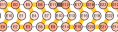
(a) Glider

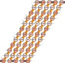
(b) Switchback

(c) Glider/Switchback turn folding compatibility.

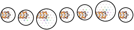
(d) from left to right: the folding of the subsequence as a glider.

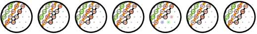
(e) from left to right: the folding of the subsequence as a switchback.

Figure 1: Glider/switchback subsequence. The folding path of the transcript is represented as the thick colorful line and the -bonds between beads are represented as dashed lines. The bond-maximizing path for the $\delta=3$ lastly produced beads is represented by a thick black line, possibly terminated by several colorful paths if several paths realize the maximum of number of bonds.

2.4 Skipping Cyclic Tag Systems and Turing-Universality

Our proof of the Turing-universality of oritatami systems consists in simulating a special kind of cyclic tag systems (CTS), called skipping cyclic tag system. Cook introduced CTS in [2] and proved that they combined the tremendous advantage of simulating efficiently any Turing machines, while not requiring a random access lookup table, which makes simulation a lot easier.

A skipping cyclic tag system (SCTS)

consists of a cyclic list of $n$ words ${\alpha=\langle{\alpha^{0},\ldots,\alpha^{n-1}}\rangle\in\{\texttt{0},\texttt{1}\}^{*}}$, called appendants, and an initial dataword $u^{0}\in\{\texttt{0},\texttt{1}\}^{*}$. Intuitively, $\alpha$ encodes the program and $u^{0}$ encodes the input. Its configuration at time $t$ consists of a marker $m^{t}$, recording the index of the current appendant at time $t$, and a dataword $u^{t}$. Initially, $m^{0}=0$ and the dataword is $u^{0}$. At each time step $t$, the SCTS acts deterministically on configuration $(m^{t},u^{t})$ in one of three ways:

(Halt step) If $u^{t}$ is the empty word $\epsilon$,

then the SCTS halts;

(Nop step) If the first letter $u^{t}_{0}$ of $u^{t}$ is 0,

then $u^{t}_{0}$ is deleted and the marker moves to the next appendant cyclically: i.e., $m^{t+1}=(m^{t}+1)\mathbin{\operatorname{mod}}n$ and ${u^{t+1}=u^{t}_{1}\cdots u^{t}_{|u^{t}|-1}}$;

(Skip-append step) If $u^{t}_{0}=\texttt{1}$,

then $u^{t}_{0}$ is deleted, the next appendant $\alpha^{(m^{t}+1\leavevmode\nobreak\ \mathbin{\operatorname{mod}}\leavevmode\nobreak\ n)}$ is appended onto the right end of $u^{t}$, and the marker moves to the second next appendant: i.e., $u^{t+1}=u^{t}_{1}\cdots u^{t}_{|u^{t}|-1}\cdot\alpha^{(m^{t}+1\leavevmode\nobreak\ \mathbin{\operatorname{mod}}\leavevmode\nobreak\ n)}$ and ${m^{t+1}=(m^{t}+2)\mathbin{\operatorname{mod}}n}$.

For example, consider the SCTS ${\mathcal{E}}=(\langle{\texttt{110},\epsilon,\texttt{11},\texttt{0}}\rangle;u^{0}=\texttt{010})$. Its execution $({}^{[m^{t}]}u^{t})_{t}$ is:

${}^{[0]}\texttt{010}\rightarrow{}^{[1]}\texttt{10}\begin{array}[]{c}{\xrightarrow{\texttt{Append}}}\\[-8.00003pt] \scriptstyle[2:\texttt{11}]\end{array}{}^{[3]}\texttt{011}\rightarrow{}^{[0]}\texttt{11}\begin{array}[]{c}{\xrightarrow{\texttt{Append}}}\\[-8.00003pt] \scriptstyle[1:\epsilon]\end{array}{}^{[2]}\texttt{1}\begin{array}[]{c}{\xrightarrow{\texttt{Append}}}\\[-8.00003pt] \scriptstyle[3:\texttt{0}]\end{array}{}^{[0]}\texttt{0}\rightarrow{}^{[1]}\,\texttt{Halt}$

Turing universality.

A sequence of articles and thesis by Cook [2], and Neary and Woods [15, 12], allows to show that SCTS are able to simulate any Turing machine efficiently in the following sense: (proof deferred to appendix A.5)

Proposition 2.2 ([15, 12]).

Let ${\mathcal{M}}$ be a deterministic Turing machine using a single tape. There is a polynomial algorithm that computes a skipping cyclic tag system ${\mathcal{S}}_{\mathcal{M}}$, together with a linear-time encoding $u_{\mathcal{M}}(x)$ of the input $x$ of ${\mathcal{M}}$ as an input dataword for ${\mathcal{S}}_{\mathcal{M}}$, such that for all input $x$: ${\mathcal{S}}_{\mathcal{M}}$ halts on input dataword $u_{\mathcal{M}}(x)$ if and only if ${\mathcal{M}}$ halts on input $x$. Furthermore, for all $t$, if ${\mathcal{M}}$ halts after $t$ steps, then ${\mathcal{S}}$ halts after $O_{\mathcal{M}}(t^{2}\log t)$ steps. Moreover, the number of appendants of ${\mathcal{S}}$ is a multiple of 4.

In order to prove Theorem 2.1, we are thus left with proving that there is an oritatami system that simulates in quadratic time any SCTS system (see Theorem B.1 in appendix for a precise statement).

3 The block simulation of SCTS: Proving the correctness of local folding is enough

Given a SCTS $\mathcal{S}$, we design an oritatami system ${\mathcal{O}}_{\mathcal{S}}$ that folds into a version, at a larger scale, of the annotated trimmed space-time diagram of ${\mathcal{S}}$ (or trimmed diagram for short) defined as follows:

Trimmed diagram of SCTS.

Any SCTS proceeds as follows: it trims all the leading 0s in the data word and then appends the currently marked appendant when it reads the first 1 (if any; otherwise it halts). It is thus natural to group all these steps (trim leading 0s and process the leading 1) as one single macro step. This motivates the following representation. Given a SCTS $(\alpha^{0},\ldots,\alpha^{n-1};u^{0})$, we denote by ${0\leqslant t_{1}<t_{2}<\cdots}$ all the times $t$ such that the dataword $u^{t}$ starts with letter 1 and set $t_{0}=-1$ by convention. Let us now group all deletion steps occurring during steps $t_{i}+1$ to $t_{i+1}-1$ by simply indicating in exponent the marker $m^{t}$ before each letter read. In the case of our STCS $\mathcal{E}$, we have $t_{0}=-1,t_{1}=1,t_{2}=3,t_{3}=4$ and its execution is now represented as:

$${}^{[0]}\texttt{0}{}^{[1]}\texttt{10}\begin{array}[]{c}{\xrightarrow{\texttt{Append}}}\\[-8.00003pt] \scriptstyle[2:\texttt{11}]\end{array}{}^{[3]}\texttt{0}{}^{[0]}\texttt{1}\texttt{1}\begin{array}[]{c}{\xrightarrow{\texttt{Append}}}\\[-8.00003pt] \scriptstyle[1:\epsilon]\end{array}{}^{[2]}\texttt{1}\begin{array}[]{c}{\xrightarrow{\texttt{Append}}}\\[-8.00003pt] \scriptstyle[3:\texttt{0}]\end{array}{}^{[0]}\texttt{0}{}^{[1]}\leavevmode\nobreak\ \texttt{Halt}$$

Now, let’s align the resulting datawords in a 2D diagram according to their common parts:

$\begin{array}[]{r@{}r@{}r@{\,}r@{\,}r@{\,}r@{\,}r@{\,}rr@{{~~\longrightarrow~~}}c@{~}r@{\,:\,}l}\lx@intercol\hfil\overset{t_{0}}{\scriptstyle\downarrow}\hfil\lx@intercol&&\lx@intercol\hfil\overset{t_{1}}{\scriptstyle\downarrow}\hfil\lx@intercol&&\lx@intercol\hfil\overset{t_{2}}{\scriptstyle\downarrow}\hfil\lx@intercol&\lx@intercol\hfil\overset{t_{3}}{\scriptstyle\downarrow}\hfil\lx@intercol\\ \cline{2-4}\cr&\vrule\,\lx@intercol\hfil{}^{[0]}\texttt{0}\,&\vrule\,\lx@intercol\hfil{}^{[1]}\texttt{1}\,&\vrule\,\lx@intercol\hfil\texttt{0}\,&\vrule\,\lx@intercol\hfil\,&&&&{\leavevmode\nobreak\ \leavevmode\nobreak\ \longrightarrow\leavevmode\nobreak\ \leavevmode\nobreak\ &{\texttt{Append}}\hfil\leavevmode\nobreak\ &[2&\texttt{11}]\\[2.0pt] \cline{2-6}\cr&&&\vrule\,\lx@intercol\hfil{}^{[3]}\texttt{0}\,&\vrule\,\lx@intercol\hfil{}^{[0]}\texttt{1}\,&\vrule\,\lx@intercol\hfil\texttt{1}\,&\vrule\,\lx@intercol\hfil\,&&{\leavevmode\nobreak\ \leavevmode\nobreak\ \longrightarrow\leavevmode\nobreak\ \leavevmode\nobreak\ &{\texttt{Append}}\hfil\leavevmode\nobreak\ &[1&\epsilon]\\[2.0pt] \cline{4-6}\cr&&&&&\vrule\,\lx@intercol\hfil{}^{[2]}\texttt{1}\,&\vrule\,\lx@intercol\hfil\,&&{\leavevmode\nobreak\ \leavevmode\nobreak\ \longrightarrow\leavevmode\nobreak\ \leavevmode\nobreak\ &{\texttt{Append}}\hfil\leavevmode\nobreak\ &[3&\texttt{0}]\\ \cline{6-7}\cr&&&&&&\vrule\,\lx@intercol\hfil{}^{[0]}\texttt{0}\,&\vrule\,\lx@intercol\hfil{}^{[1]}\,&{\leavevmode\nobreak\ \leavevmode\nobreak\ \longrightarrow\leavevmode\nobreak\ \leavevmode\nobreak\ &{\texttt{Halt}}\hfil\leavevmode\nobreak\ &[1&\epsilon]\\[2.0pt] \cline{7-7}\cr\end{array}}}}}$

This defines the annotated trimmed space-time diagram for the SCTS $\mathcal{E}$. Lemma A.1 in appendix provides the formal definition for an arbitrary SCTS.

The transcript.

The proof of Theorem B.1 relies on constructing a transcript (and a fixed rule) that will reproduce faithfully the trimmed diagram of the simulated STCS. Figure 2 illustrates the folded configuration of the transcript corresponding to SCTS $\mathcal{E}$. Macroscopically, the transcript folds into a zig-zag sequence of blocks, each performing a specific operation.

The current dataword

is encoded at the bottom of each row of blocks: 0s are encoded by a spike, and 1s are encoded by a flat surface.

the seed configuration

encodes the initial dataword and opens the first zig row at which the folding of the transcript starts. Letters 0 and 1 are encoded by a spike (see Fig. 3(a)) and a flat surface (see Fig. 3(b)) respectively.

in each zig row (left to right),

the transcript folds into a series of Read0

$\blacktriangleright$ blocks (trimming the leading 0s from the dataword encoded above), then into a Read1

$\blacktriangleright$ block, if the dataword contains a 1, or into a Halt block terminating the folding, otherwise; this is the zig-up phase. Then, the transcript starts the zig-down phase which consists in folding into Copy

$\blacktriangleright$ block copying the letters encoded above to the bottom of the row; once the end of the dataword is reached, the transcript folds into an Append

$${\makebox[6.00006pt]{\scalebox{0.8}{\makebox[0.0pt]{\raisebox{3.99994pt}[0.0pt]{$\blacktriangleright$}}\makebox[0.0pt]{\raisebox{0.0pt}[0.0pt]{$\blacktriangleleft$}}}}}Return$$

block which encodes, at the bottom of the row, the currently marked appendant, and finally, opens the next zag row.

in each zag row (right to left),

the transcript folds into Copy

$\blacktriangleleft$ blocks copying the dataword encoded above to the bottom of the row. For the leftmost letter, the transcript folds into the special Copy

$\blacktriangleleft$$\blacktriangleright$ LineFeed block which also opens the next zig row.

(a) Folding of the oritatami system simulating the STCS $\mathcal{E}$.

Read0$\blacktriangleright$ Read1$\blacktriangleright$ Copy0$\blacktriangleright$Unit Copy1$\blacktriangleright$Unit Halt Append $\blacktriangleright$$\blacktriangleleft$ Return  LineFeed $\blacktriangleleft$$\blacktriangleright$ Unit

(b) Exploded view of the bricks and modules inside the blocks involved in the simulation above.

Figure 2: Folding of the transcript simulating the STCS $\mathcal{E}$, and some block internal structures.

The transcript is a periodic sequence whose period is the concatenation of $n$ bead type sequences ${\scalebox{0.8}{\framebox{\leavevmode\hbox{\set@color\resizebox{}{}{{\leavevmode\hbox{\set@color{{Appendant $\alpha^{0}$}}}}}}}}},\ldots,{\scalebox{0.8}{\framebox{\leavevmode\hbox{\set@color\resizebox{}{}{{\leavevmode\hbox{\set@color{{Appendant $\alpha^{n-1}$}}}}}}}}}$ called segments, each encoding one appendant.

Encoding of the marker.

Read

$\blacktriangleright$ and Append

$${\makebox[6.00006pt]{\scalebox{0.8}{\makebox[0.0pt]{\raisebox{3.99994pt}[0.0pt]{$\blacktriangleright$}}\makebox[0.0pt]{\raisebox{0.0pt}[0.0pt]{$\blacktriangleleft$}}}}}Return$$

blocks consist of the folding of exactly one segment, whereas Copy

$\blacktriangleright$, Copy

$\blacktriangleleft$ and Copy

$\blacktriangleleft$$\blacktriangleright$ LineFeed consist of the folding of exactly $n$ segments. It follows that the appendant encoded in the leading segment folded inside each block corresponds to the currently marked appendant in the simulated SCTS. As a consequence, the appendant contained in the folded Append

$${\makebox[6.00006pt]{\scalebox{0.8}{\makebox[0.0pt]{\raisebox{3.99994pt}[0.0pt]{$\blacktriangleright$}}\makebox[0.0pt]{\raisebox{0.0pt}[0.0pt]{$\blacktriangleleft$}}}}}Return$$

block is indeed the appendant to be appended to the dataword.

The segment sequence.

Each segment Appendant $\alpha^{i}$ encodes the appendant $\alpha^{i}$ as a sequence of $6+|\alpha^{i}|$ modules: one of each module A , B , and C , then $|\alpha^{i}|$ of module D , then one of each module E , F and G . Each module is a bead type sequence that plays a particular role in the design:

Module A

folds into the initial scaffold upon which the next modules rely.

Module B

detects if the dataword is empty: if so, it folds to the left and the folding gets trapped in a closed space and halts; otherwise, it folds to the right and the folding continues.

Module C

detects the end of the dataword and triggers the appending of the marked appendant accordingly.

Module D

encodes each letter of the appendant.

Module E

ensures by padding that all appendant sequences have the same length when folded (even if the appendant have different length). It serves two other purposes: Module B senses its presence to detect if the dataword is empty; and its folding initiates the opening the zag row once the marked appendant has been appended to the dataword.

Module F

is the scaffold upon which Module G folds. It is specially designed to induce two very distinct shapes on G depending on the initial shift of G . Furthermore, when Module F is exposed, Module C folds along F which triggers the appending of the marked appendant encoded by the modules D following C .

Module G

is the “logical unit” of the transcript. It implements three distinct functions which are triggered by its interactions with its environment: Reading the leading letter of the dataword, Copying a letter of the dataword, and Opening the next zig row at the leftmost end of a zag row.

We call bricks the folding of each of these modules. The blocks into which the transcript folds, depend on the bricks in which its modules fold, as illustrated in Fig. 2(b). Please refer to sections C to LABEL:sec:all:bricks:full in appendix for the description of blocks in terms of bricks and of how they articulate with each other to produce the desired macroscopic folding pattern.

The full description of each of these sequences is given in Section LABEL:sec:all:bricks:full in appendix.

Let ${\mathcal{S}}=(\alpha^{0},\alpha^{1},\ldots,\alpha^{n-1};u^{0})$ be a skipping cyclic tag system, and, as before, let for all integer $i\geqslant 0$, $t_{i}$ be the $i^{\text{th}}$ step where $u^{t}$ starts with 1 (starting from $0$, i.e. $t_{0}$ is the first step where $u^{t_{0}}$ starts with 1). The following lemma shows that the transcript described above folds indeed into blocks that simulates the trimmed diagram of $\mathcal{S}$. Proposition 2.2 and Theorem B.1 are direct corollaries of this lemma.

Lemma 3.1 (Key lemma).

There is a bead type set $B$ and a rule such that: for every SCTS ${\mathcal{S}}$, there are $\pi_{\mathcal{S}}$ and $(\sigma_{\mathcal{S}},s_{\mathcal{S}})$ defined as in Theorem 2.1 such that, for every initial dataword $u^{0}$, the (possibly infinite) final folded path of the oritatami system ${\mathcal{O}}_{\mathcal{S}}=((\pi_{\mathcal{S}})^{\infty},\mathbin{{\color[rgb]{1,0,0}\varheart}},\delta=3)$ from the seed configuration $(\sigma(u^{0}),s(u^{0}))$ is exactly structured as the following sequence of blocks organized in zig and zag rows as follows: (recall Fig. 2(a))

• First, the block $\textsf{Seed}(\texttt{$u^{0}$})$ ending at coordinates $(-1,0)$.

• Then, for $i\geqslant 0$, the $i$-th row consists of a zig row located between $y=2(i-1)h+1$ and $y=2ih$, and a zag row located between $y=2ih+1$ and $y=2(i+1)h$, composed as follows:

  $\bullet$ (Compute) if $u^{1+t_{i}}=\texttt{0}^{r}1\cdot s$ and if $s\neq\epsilon$ or $\alpha^{1+i+t_{i+1}}\neq\epsilon$:

  then ${r=t_{i+1}-t_{i}-1}$ and:

  • the $i$-th zig-row consists from left to right of the following sequence of blocks whose origins are located at the following coordinates:
    

    $\begin{array}[]{cccccccccc}\swarrow y&\lx@intercol\hfil 2ih\hfil\lx@intercol&&\lx@intercol\hfil(2i-1)h+1\hfil\lx@intercol\\ \cline{1-5}\cr\cline{7-10}\cr\rightarrow x&ih+(1+t_{i})W&\cdots&ih+(t_{i+1}-1)W&ih+t_{i+1}W&&ih+(1+t_{i+1})W-1&\cdots&ih+(|s|+t_{i+1})W-1&ih+(1+|s|+t_{i+1})W-1\\ \hline\cr\hline\cr\textup{Blocks}&\textsf{Read{{{0}$$}}$\blacktriangleright$}&\cdots&\textsf{Read{{{0}$$}}$\blacktriangleright$}&\textsf{Read{{{1}$$}}$\blacktriangleright$}&&\textsf{Copy{{$(s_{0})$$$}}$\blacktriangleright$}&\cdots&\textsf{Copy{{$(s_{|s|-1})$$$}}$\blacktriangleright$}&\textsf{Append$[\alpha^{1+i+t_{i+1}}]${\makebox[6.00006pt]{\scalebox{0.8}{\makebox[0.0pt]{\raisebox{3.99994pt}[0.0pt]{$\blacktriangleright$}}\makebox[0.0pt]{\raisebox{0.0pt}[0.0pt]{$\blacktriangleleft$}}}}}Return}{}\\ \hline\cr\textup{Marker}&i+1+t_{i}&\cdots&i+r+t_{i}&i+t_{i+1}&&i+1+t_{i+1}&\cdots&i+1+t_{i+1}&i+1+t_{i+1}\end{array}$

    
    

    This row ends at position $((i+1)h+(1+|s|+|\alpha^{i+1+t_{i+1}}|+t_{i+1})W-7,2ih+2)$.

  • the $i$-th zag-row consists from right to left of the following sequence of blocks whose origins are located at the following coordinates:
    

    $\begin{array}[]{ccccc}\swarrow y&\lx@intercol\hfil 2ih+1\hfil\lx@intercol\\ \hline\cr\rightarrow x&(i+1)h+(2+t_{i+1})W-8&(i+1)h+(3+t_{i+1})W-8&\cdots&(i+1)h+(1+|v|+t_{i+1})W-8\\ \hline\cr\hline\cr\textup{Blocks}&\textsf{Copy{{$(v_{0}$)$$}}{\makebox[6.00006pt]{\scalebox{0.8}{\makebox[0.0pt]{\raisebox{3.99994pt}[0.0pt]{$\blacktriangleleft$}}\makebox[0.0pt]{\raisebox{0.0pt}[0.0pt]{$\blacktriangleright$}}}}}LineFeed}&\textsf{Copy{{$(v_{1})$$$}}$\blacktriangleleft$}&\cdots&\textsf{Copy{{$(v_{|v|-1})$$$}}$\blacktriangleleft$}\\ \hline\cr\textup{Marker}&i+2+t_{i+1}&i+2+t_{i+1}&\cdots&i+2+t_{i+1}\end{array}$

    
    

    where ${v=u^{1+t_{i+1}}=s\cdot p_{i+1+t_{i+1}}}\neq\epsilon$ (as $s$ and $\alpha^{i+1+t_{i+1}}$ are not both $\epsilon$). This row ends at position $((i+1)h+(1+t_{i+1})W-1,2(i+1)h)$.

  $\bullet$ (Halt 1) if $u^{1+t_{i}}=\texttt{0}^{r}1$ and $\alpha^{1+i+t_{i+1}}=\epsilon$:

  then $r=t_{i+1}-t_{i}-1$ and the last rows of the configuration consists from left to right of the following sequence of blocks located at the following coordinates:
  

  $\begin{array}[]{ccccccccc}\swarrow y&\lx@intercol\hfil 2ih\hfil\lx@intercol&&(2i-1)h+1&&2(i+1)h\\ \cline{1-5}\cr\cline{7-7}\cr\cline{9-9}\cr\rightarrow x&ih+(1+t_{i})W&\cdots&ih+(t_{i+1}-1)W&ih+t_{i+1}W&&ih+(1+t_{i+1})W-1&&(i+1)h+(1+t_{i+1})W\\ \hline\cr\hline\cr\textup{Blocks}&\textsf{Read{{{0}$$}}$\blacktriangleright$}&\cdots&\textsf{Read{{{0}$$}}$\blacktriangleright$}&\textsf{Read{{{1}$$}}$\blacktriangleright$}&&\textsf{CarriageReturn{\makebox[6.00006pt]{\scalebox{0.8}{\makebox[0.0pt]{\raisebox{3.99994pt}[0.0pt]{$\blacktriangleright$}}\makebox[0.0pt]{\raisebox{0.0pt}[0.0pt]{$\blacktriangleleft$}}}}}LineFeed{\makebox[6.00006pt]{\scalebox{0.8}{\makebox[0.0pt]{\raisebox{3.99994pt}[0.0pt]{$\blacktriangleleft$}}\makebox[0.0pt]{\raisebox{0.0pt}[0.0pt]{$\blacktriangleright$}}}}}}{}&&\textsf{Halt}\\ \hline\cr\textup{Marker}&i+1+t_{i}&\cdots&i+t_{i+1}-1&i+t_{i+1}&&i+1+t_{i+1}&&i+2+t_{i+1}\end{array}$

  
  

  $\bullet$ finally, (Halt 2) if $u^{1+t_{i}}=\texttt{0}^{r}$ for some $r\geqslant 0$:

  then the $i$-th zig-row is last row of the configuration and consists of the following sequence of blocks located at the following coordinates:
  

  $\begin{array}[]{ccccc}\swarrow y&\lx@intercol\hfil 2ih\hfil\lx@intercol\\ \hline\cr\rightarrow x&ih+(1+t_{i})W&\cdots&ih+(r+t_{i})W&ih+(1+r+t_{i})W\\ \hline\cr\hline\cr\textup{Blocks}&\textsf{Read{{{0}$$}}$\blacktriangleright$}&\cdots&\textsf{Read{{{0}$$}}$\blacktriangleright$}&\textsf{Halt}{}\\ \hline\cr\textup{Marker}&i+1+t_{i}&\cdots&i+r+t_{i}&i+r+1+t_{i}\end{array}$

The following sections are dedicated to the proof of Key Lemma 3.1.

4 Advanced Design Tool box

In this section, we present several key tools to program Oritatami design and which we believe to be generic as they allowed us to get a lot of freedom in our design.

4.1 Implementing the logic

As in [5], the internal state of our “molecular computing machinery” consists essentially of two parameters: 1) the position inside the transcript of the part currently folding; and 2) the entry point of transcript inside the environment. Indeed, depending on the entry point or the position inside the transcript, different beads will be in contact with the environment and thus different functions will be applied as a result of their interactions. This happens during the zig phase: in the first (zig-up) part, the transcript starts folding at the bottom, forcing the modules G to fold into $\text{G}\operatorname{\raisebox{1.69998pt}{$\underline{\blacktriangleright}$}}\text{Read}$ bricks; whereas during the second (zig-down) part, the transcript starts folding at the top, forcing the modules G to fold into $\text{G}\operatorname{\overline{\blacktriangleright}}\text{Copy}$ bricks instead. Similarly, the memory of the system consists of the beads already placed on the surrounding of the area currently visited (the environment). This happens in every row of the folding: depending on the letter encoded at the bottom of the row above, the modules G fold into $\text{G}\operatorname{\raisebox{1.69998pt}{$\underline{\blacktriangleright}$}}\text{Read{0}}$ or $\text{G}\operatorname{\raisebox{1.69998pt}{$\underline{\blacktriangleright}$}}\text{Read{1}}$ bricks (zig-up phase), $\text{G}\operatorname{\overline{\blacktriangleright}}\text{Copy{0}}$ or $\text{G}\operatorname{\overline{\blacktriangleright}}\text{Copy{1}}$ bricks (zig-down phase), and $\text{G}\operatorname{\overline{\blacktriangleleft}}\text{Copy{0}}$ or $\text{G}\operatorname{\overline{\blacktriangleleft}}\text{Copy{1}}$ bricks (zag phase).

At different places, we need the transcript to read information from the environment and trigger the appropriate folding. This is obtained through different mechanisms.

Default folding.

By default, during the zig-up phase, B is attracted to the left by F and folds to the right only in presence of E above. This allows to continue the folding only if the tape word is not empty or to halt it otherwise (see Figure LABEL:fig:B:brick:ZigUp in appendix).

Geometry obstruction.

An typical example is illustrated by G . During the zig-up phase where the absence of environment below the block $Read ▶allows G tofolddownwardatthebeginning(seeFigureLABEL:fig:G:brick:Read0)whichshiftthetranscriptby7beadsalong F resultingin G toadopttheglider−shape(moredetailsonthismechanisminthenextsection).Whereasduringthezig−downphase, G cannotmakethisloopbecauseitisoccupiedbyapreviouslyplaced G .Thisresultsinaperfectalignmentof G with F whosestrongattractionforces G toadopttheswitchbackshape(seeFigureLABEL:fig:G:brick:ZigCopy0).Geometry of the environment.item item Geometry of the environment.Figure3showshowtheshapeoftheenvironmentisusedtochangethedirectionof G inglider−shape.ThisresultsinmodifyingtheentrypointintheenvironmentandallowstheOritatamisystemtotrimtheleading0sinthetapewordbygoingbacktothesameentrypoint(Fig.3(a)),switchfromzip−uptozig−downphasewhenreadinga1byopeningthenextblockfromthetop(Fig.3(b)),andfromzagtozig−upphasewhenithasrewindtothebeginningofthetapeword,bygettingdowntothebottomofthenextzigrow(Fig.3(c)).  (a) G bounces southeastward in presence of a spike encoding a 0 and folds into G¯▶Read0 . (b) G bounces eastward on a flat surface encoding a 1, and folds into G¯▶Read1 . (c) G goes straight southwestward in absence of obstacle, and folds into G◀▶LineFeed . Figure 3: The interactions of module G in “glider”-mode with different environments result in heading to different entry points to the next area of the folding.   4.2 Easing the design: getting the freedom you need Several key tools allowed to ease considerably our design, and even in some cases to make it feasible. These tools are generic enough to be considered as programming paradigms. One main difficulty we faced is that the different functions one wants to implement tend to concentrate at the same “hot-spots” in the transcript. A typical example is the midpoint of G where one wants to implement all the functions: Read, Copy and Line Feed. The following powerful tools allow to overcome these difficulties: Socks work by letting a glider/switchback module fold into a switchback turn conformation for some time when it would otherwise fold into a glider. Examples are given in Figure 4. They are easy to implement: indeed, the socks naturally adopt the same shape as the corresponding switchback turn and require thus no extra interfering bonds. They allow a lot of freedom in the design, for several reasons: First, they simplify the design of important switchback part by lifting the need for implementing the glider configuration for that part, as shown in Figure 4(a). Second, a glider naturally progresses at speed 1/3. Adding a sock allows us to slow its progression down to speed 1/5 for some time (see Fig. 4(b)) and therefore to realign them. We used that feature repeatedly to “shift” some modules: starting the folding at an initial speed-1 (i.e. straight line) and then compensating for that speed later on by introducing socks (see Fig. 4(b)). This is a key point in our design, as it allowed us to spread apart the Read and Copy functions into different subsequences of module G , and therefore to get less constraints on our rule design. In the specific case of module G , the Copy-function occurs at the center of the module, while the Read-function is implemented earlier in module! (see section LABEL:sec:full:description:G for full details) Finally, socks allow to prevent unwanted interactions between beads by concealing potentially harmful beads in unreachable area as in Figure 4(c). (a) Easing the design of switchback/glider by letting the switchback (in green) folds in its natural shape at its extremities even in “glider”-mode. (b) Module G : Realigning a pattern by slowing its folding down at the end to compensate speeding it at the beginning. (c) Module D : Preventing unwanted interactions between the beads outlined in red and the ones below, by concealing the red ones on top of the glider. Figure 4: Different uses of socks: (a) Easing bond design; (b) Delaying; (c) Preventing unwanted interactions. Exponential bead type coloring is a key tool to allow module G to fold into different shapes, glider or switchback, along module F , when folding in the Read ▶configuration.Theproblemitsolvesisthatinorderfor G tofoldintoswitchbacks,weneedstronginteractionsbetween G anditsneighboringmodule F (seeFig.LABEL:fig:G:brick:Read0),whereasinorderfor G tofoldasglider,wewanttoavoidthoseinteractions(seeFig.LABEL:fig:G:brick:ZigCopy0).Thisismadepossiblebecauseglidersprogressatspeed1/3whileswitchbacksprogressatspeed1.Usingapower-of-3coloring,wemanagetoeasilyachievethesecontradictinggoalsaltogether(theconstructionisanalysedinLemmaLABEL:lem:exp:colinSectionLABEL:sec:enum:env). 5 Correctness of local folding: Proof tree certificates The goal of this section is to conclude the proof of our design by proving Key Lemma 3.1. The proof works by induction, assuming that the preceding beads of the transcript fold at the locations claimed by the lemma. We proceed in 3 steps: • We first enumerate all the possible environments for every part of the transcript. As, we carefully aligned our design, most of the beads only see a small number of different environments. • For the few cases (three in total) where the number of environments is unbounded, we give an explicit proof of correctness of their folding (Lemmas LABEL:lem:env:below:write, LABEL:lem:env:top:read1, and LABEL:lem:exp:col in section LABEL:sec:enum:env). This is where the concealing feature of socks and the exponential bead type coloring play a crucial role. • For all the other cases, we designed human-checkable computer-generated certificates, called proof trees. It consists in listing in a compact but readable manner all the possible paths for the transcript in every possible environment. In order to match human readability, paths with identical bonding patterns are grouped into one single ball. Balls containing the paths maximizing the number of bonds are highlighted in bold and organized in a tree. This reduces the number of cases to less than 5 balls in most of the levels of the tree, achieving human-checkability of the computed certificate (see Fig. 5 in appendix). Proof trees are available at https://www.irif.fr/~nschaban/oritatami/ This ensures the highest level of certification of the correctness of our design. (a) Proof tree for the glider turn in G¯▶Read0 . (b) Proof tree for the glider turn in G¯▶Read1 . Figure 5: Two examples of proof trees for the same subsequence in two different environements. The number at the upper-left corner of every ball stands for the number of bonds for the path inside the ball. The number at the lower right corner of each ball stands for the number of paths grouped in the ball, allowing to check that no path was omitted. Balls highlighted in black bold contain the bonds-maximizing paths. Balls highlighted in grey bold contain the paths that places the bead at the same location as the bonds-maximizing paths, and which must thus be considered in the next level as well. Please find next the omitted part of article due to space constraints. Appendix A Skipping Cyclic Tag Systems Notations. We index the letters of every word u=u0…u|u|-1 from 0 to |u|-1. Given two words u and v, we denote by u⋅v their concatenation: u⋅v=u0…u|u|-1v0…v|v|-1. We denote by u∞ the oneway infinite periodic word u⋅u⋯. For all i⩽j, we denote by ui..j the (possibly empty) factor umax(0,i)…umin(j,|u|-1). The empty word is denoted by ϵ. The indices in the notation OL() where L is a list of variables (for instance L=A,B) indicates that the constant in the O() only depends on the variable in L (for instance A and B) and on no other values. A.1 Trimmed diagram The following lemma gives the formal description of the trimmed diagram of a SCTS (α;u0) with marker mt. Recall that ti is the i-th time t such that the dataword ut starts with letter 1 (t0=-1 by convention). Lemma A.1. The annotated word on the row i (indexed from i=0) of the trimmed diagram is: (the markers in exponent are computed modulo n) •  if u1+ti=0r1⋅s for some r⩾0 and s∈{0,1}∗: then, r=ti+1-ti-1 and the annotated word on row i is [i+1+ti]0⋯[i-1+ti+1]0[i+ti+1]1⋅s whose first letter is placed in column ti+1 (assuming the leftmost column is indexed by 0); •  if u1+ti=0r for some r>0: then, row i is the last row of the diagram and its annotated word is [i+1+ti]0⋯[i+ti+r]0[i+ti+r+1] and starts at column ti+1. Proof A.2 (Proof sketch). Simply observe that mti=i+timodn, as indeed exactly ti letters have been read and exactly i appending steps have occurred before reading the i-th 1. A.2 Turing-universality of Skipping Cyclic Tag Systems This proof makes use of the time-efficient reduction from Turing machines to cyclic tag systems (CTS) designed in [12, Theorem 4.3.2 p. 65], improving on [2, 15]. A cyclic tag system C=(α0,…,αn-1;v0) consists of a list of n appendants α0,…,αn-1∈{0,1}∗ and an initial dataword v0∈{0,1}∗. Its configuration at time t consists of a marker mt=tmodn, recording the index of the current appendant at time t, and a dataword vt. Initially, m0=0 and the dataword is v0. At each time step t, the CTS acts deterministically on configuration (mt,vt) in one of three ways: (Halt step) If vt is the empty word ϵ, then the CTS halts; (Nop step) If the first letter vt0 of vt is 0, then vt0 is deleted and the marker moves to the next appendant cyclically: i.e., mt+1=(mt+1)modn and vt+1=vt1⋯vt|vt|-1; (Append step) If vt0=1, then vt0 is deleted, the currently marked appendant α(mtmodn) is appended onto the right end of vt: i.e., vt+1=vt1⋯vt|vt|-1⋅α(mtmodn) and mt+1=(mt+1)modn (no skipping). According to the definition in [12, 2, 15], the computation of a CTS is said to end if either the dataword is ϵ or if it repeats a configuration. This relaxed definition of termination was introduced for the purpose of reducing any Turing machine to cellular automaton rule 110, whose computation never halts. Precisely, [12, Theorem 4.3.2, p. 65] states the following: let M be any deterministic Turing machine using a single tape; there is a cyclic tag system CM with appendants α0,…,αn-1 and a linear-time encoding vM of the input x of M, such that for all input x: (1) CM halts from initial dataword vM(x) if and only if M halts from input x; and (2) for all t, if M halts after t steps on x, then TM halts after OM(t2logt) steps on vM(x). For our purpose, we need the computation of the CTS to stop with an empty dataword (and not to enter a cycle) if the simulated Turing machine stops, precisely: Lemma A.3 (Corollary of Theorem 4.3.2 in [12]). For every Turing machine M, there is CTS ^CM and a linear time encoding ^vM(x)=χ(vM(x)) that encodes any input x of M into an initial dataword ^v0=^vM(x) such that: (1) ^CM halts from ^v0 with an empty dataword iff M halts from input x; and (2) if M halts after t steps from x, then ^CM after O(t2logt) steps from ^v0. Proof A.4. We proceed as follows by defining a CTS ^CM “with two processing modes”: the first mode emulates CM, the second mode just erases the data word; switching from one mode to the other just requires inserting a single letter 0 in the dataword. Consider χ the homomorphism on {0,1}∗ such that χ(0)=00 and χ(1)=01, i.e. χ inserts a 0 before every letter of a word. Then, consider the CTS ^CM with 2n appendants: ^α2i+1=χ(^αi) and ^αM2i=ϵ, for 0⩽i<n. An immediate induction shows that ^CM simulates CM exactly twice slower, indeed: if vt and ^vt denote the datawords of CM and ^CM starting from the initial datawords v0 and ^v0=χ(v0) respectively, then for all time t, ^v2t=χ(vt). Now, if we shift the dataword of ^CM by one letter, the appendants that will be appended next, are all the empty word ϵ, and the dataword will be completely erased, yielding to the desired terminaison. Without loss of generality, we assume that M has an unique final state qF. According to the design of CM in the proof Theorem 4.3.2 p. 65 in [12], for every step t of M where the configuration is ⋯B⋯Bσ1…σj[q,d]σj+1σj+2⋯σs-2B⋯B⋯ (i.e., where the head is over position σj+1, the current state is q and the next head movement is d, B denotes the blank symbol), the dataword of CM is, at the step O(t2logt) corresponding to first stage of the processing of this configuration by CM: ⟨1,q,d⟩⟨σj+1⟩⋯⟨σs-2⟩⟨σB⟩μs′⟨σ1⟩⋯⟨σj⟩ and the marker is 0. Each ⟨⋅⟩ and μ stands for a binary encoding containing a single 1. Furthermore, there is at most one pattern ⟨1,q,d⟩ in the dataword of CM at all time. Let i be the index of the only 1 in ⟨1,qF,d⟩. We then change the appendant ^α2i+1 to 0. It follows that, the first time the pattern χ(⟨1,qF,d⟩) appears, i.e. the first time the simulated Turing machine M enters the final state, the CTS ^CM switches to the even-indexed empty-appendants-mode, then erases the whole dataword, and halts with an empty dataword, as desired. Furthermore, if M halts after t steps, ^CM halts after O(t2logt) steps. We now show how to simulate the CTS ^CM with a SCTS. Proof A.5 (Proof of Proposition 2.2). The original cyclic tag system by Cook [2] differs from the skipping cyclic tag system only in that in the original, the list rotates by 1 no matter which letter the current word begins with. Consider the CTS ^CM, given by the lemma above, with 2n appendants ^α0,…,^α2n-1, together with its linear-time input encoding ^vM. Let χ′ be the homomorphism over {0,1}∗ defined as χ′(0)=00 and χ′(1)=1. Let SM be the SCTS with 4n appendants: β2i=ϵ and β2i+1=χ′(^αi) for 0⩽i<2n. An immediate recurrence shows that SM simulates ^CM, precisely: if vt and ut denote respectively the datawords of ^CM and SM with initial datawords v0∈{0,1}∗ and u0=χ′(v0) then, for all time t, ut+rt=vt where rt is the number of 0s read by ^CM up to time t (note that rt⩽t). Let uM(x)=χ′(^vM(x)) denote the linear time encoding of the input x of M as the initial dataword of SM. It follows that (1) SM halts from input dataword uM(x) iff M halts from input x; and (2) if M halts from input x after t steps, then SM halts from uM(x) with an empty dataword after O(t2logt) steps. Note that moreover, the number of appendants of SM is a multiple of 4. Appendix B Proof of main Theorem 2.1 as a consequence of key Theorem B.1 The remaining of this article is dedicated to prove the following theorem which implies Theorem 2.1 by the proposition above (see appendix B.2). Theorem B.1 (Key theorem). There is a fixed set B of 542 bead types and a fixed attraction rule  on B together with two polynomial-time encodings: • π that maps any SCTS S with n⩾8 appendants α=⟨α0,…,αn-1⟩ where n is a multiple of 4, to a bead-type sequence πS∈B∗ of exact length: |πS|=18Kn(Kn+12n-8)+3n(192n-171)+30∑i=0n-1|αi|=O(|α|4) where K=L+12-(Lmod2)⩽L+12 with L=maxi|αi| being the length of the longest appendant, and |α|=∑i=0n-1|αi|. Note that πS only depends on the appendants of S. • (sS,σS) that maps any input dataword u of S to a seed configuration σS(u) of a bead type sequence sS(u) of length OS(|u|), precisely: |σS(u)|=2|u|(3K+16)+|u|0+9K(n-1)+36n-21=OS(|u|) where |u|0=#{i:ui=0} is the number of 0s in u, such that: For any SCTS S with n⩾8 appendants, where n is a multiple of 4, and every input dataword u of S, the deterministic and periodic oritatami system OS=((πS)∞,,3) with bead type sequence (πS)∞ and delay δ=3, halts when folding from seed configuration σS(u) if and only if S halts on input dataword u. Furthermore, for all t, if S halts on u after t steps, then the folding OS from seed configuration σS(s) halts after folding OS(t2) beads. Note that requiring that n⩾8 and n being a multiple of 4 does not restrict this result. Indeed, repeating the appendants sequence k times in a SCTS, yields a strictly identical SCTS with k times the number of appendants. These requirements are however necessary to ensure the proper folding alignment in the design of our oritatami system. Proof B.2 (Proof of Theorem 2.1). Consider a universal Turing machine M and the skipping cyclic tag system SM provided by Proposition 2.2 together with its linear-time input encoder uM. Consider the set of 542 bead types B, the rule , the oritatami system OM=((πM)∞,,3) whose primary structure has period πM=πSM, and the linear-time seed encodings (sSM,σSM) provided by Theorem B.1 when applied to SM. Let us define for short sM(x)=sSM(uM(x)) and σM(x)=σSM(uM(x)), the seed bead types sequence and the seed conformation of OM corresponding to the input x of M. Then, by construction: 1. For all input x of M, M halts on input x, if and only if SM halts on input dataword uM(x), if and only if OM halts its folding from seed conformation σM(x)=σSM(uM(x)). 2. For all input x of M and all time t, if M halts on x after t steps, then SM halts on input dataword uM(x) after T=OM(t2logt) steps, and thus OM halts its folding from seed conformation σM(x) after OSM(T2)=OM(t4log2t) steps. 3. For all input x of M, the length of the seed conformation encoding x in OM is OSM(|uM(x)|)=OM(|x|), linear in |x|. 4. Finally, the oritatami system OM and seed encoding (sM,σM) are obtained in polynomial time from the skipping tag system SM, which is also obtained in polynomial time from M. The reduction is thus computed in polynomial time. Appendix C Folding paths of all the bricks of our design This section presents all the bricks, i.e. all the folding paths of the 7 modules (i.e. subsequences of the transcript) composing each unit of the transcript. The folding of each module into one of these bricks depending on the context, is the key to the correctness of the folding of our transcript design into the shape of the trimmed diagram the simulated STCS as stated in Lemma 3.1. This section just presents the shape of each brick for each module together with an illustration to scale. Its purpose is to provide a guideline to the description of the blocks in the next section. The full description of each brick will be given in section LABEL:sec:all:bricks:full. To ease the reading, the brick name contains a specific symbol indicating to which kind of phase of the folding the brick belongs: • Zig-up bricks are annotated by ¯▶ • Zig-down bricks are annotated by ¯▶ • Appending bricks are annotated by ​✎ • Carriage-return bricks (spanning from a zig row to the next zag row) are annoted by ▶◀ • Zag bricks are annotated by ¯◀ • Line-feed bricks (spanning from a zag row to the next zig row) are anoted by ◀▶ • Halting bricks are annotated by ■ The subsequences corresponding to each of the 7 modules are referred by A , B , C , D(x)r,t , Ea , F , G . Some modules ( D and E ) have parameters that will be explained later, in the next sections. Their bricks, i.e. their possible folding depending on the context are referred by: Module A (see section C.1): A¯▶ (zig-up), A¯▶ (zig-down) and A¯◀ (zag). Module B (see section C.2): B¯▶ (zig-up), B¯▶ (zig-down), B¯◀ (zag) and B■ (halt). Module C (see section C.3): C¯▶ (zig-up), C¯▶ (zig-down), C¯◀ (zag) and C¯▶End (zig-up, enf of dataword detected). Module D(x)r,t (see section C.4): D(x)r,t¯▶ (zig-up), D(x)r,t¯▶ (zig-down), D(x)r,t¯◀  (zag) and  ​✎D(x)r,t​ (append). Module Ea (see section C.5): Ea¯▶ (zig-up), Ea¯▶ (zig-down), Ea¯◀ (zag) and Ea▶◀  (carriage return). Module F (see section C.6): F¯▶ (zig-up), F¯▶ (zig-down) and F¯◀ (zag). Module G (see section C.7): G¯▶Read0 (read 0), G¯▶Read1 (read 1), G¯▶Copy0 (zig-down), G¯▶Copy1 (zig-down), G¯◀Copy0 (zag), G¯◀Copy1 (zag), and G◀▶LineFeed (line feed). In the following figures, a lighter and a darker grey arrow indicates the beginning and the end of the folding path of each brick respectively. The parameter h will be defined later and refers to the height of the blocks composing the folded shape of our design. C.1 All bricks for Module A Module A always folds as a glider of height h and width 3, pointing to NE in zig-up phase, SE in zig-down phase and SW in zag phase. The folding of module A serves as a scaffold for the folding of the next modules in the zig-up and zig-down phases. All its possible bricks are displayed in Fig. 6. (a) The brick A¯▶ . (b) The brick A¯▶=HorizontalMirror(A¯▶). (c) The brick A¯◀=Rotate180∘(A¯▶). Figure 6: Folding paths to scale of all the bricks for Module A (see section LABEL:sec:full:description:A for full description). C.2 All bricks for Module B Module B is 5 beads long. It folds along the preceding brick of Module A : • to the right in zig-down; • to the left in zag phase; • to right in zig-up phase if the dataword encoded in the zag-row above is not empty; • but to the left in the zig-up phase if the dataword encoded above is empty (terminating the folding as it is now trapped in a closed area). All its possible bricks are displayed in Fig. 7. Note that B¯▶=HorizontalMirror(B¯▶) and B¯◀=Rotate180∘(B¯▶). (a) The brick B¯▶ . (b) The brick B¯▶ . (c) The brick B¯◀ . (d) The brick B■ . Figure 7: Folding paths to scale of all the bricks for Module B (see section LABEL:sec:full:description:B for full description). C.3 All bricks for Module C Module C folds in switchbacks of height almost h, along the brick of the preceding module A : • in 3 switchbacks in the zag phases; • in 3 switchbacks in the zig-up or zig-down phases if the current folding did not reach the end of the dataword encoded in the zag-row above yet; • but in 2 switchbacks ( C¯▶End ) if this end is reached, creating the initial condition for folding the next modules as the encoding of the letters of the appendant to be appended at this stage of the simulation. All its possible bricks are displayed in Fig. 8. (a) The brick C¯▶ . (b) The brick C¯▶=HorizontalMirror(C¯▶). (c) The brick C¯◀=Rotate180∘(C¯▶). (d) The brick C¯▶End . Figure 8: Folding paths to scale of all the bricks for Module C (see section LABEL:sec:full:description:C for full description). C.4 All bricks for Module D Module D(x)r,t is used to encode each letter of the appendant stored in each block unit. Its parameters x,r,t stands for the letter x∈{0,1} and the position index of that letter in the encoded appendant (r says if it is either at the first, odd or even, and t if it is the last or not). All these variants of module D fold slightly differently. Module D(x)r,t folds either: • in 6 switchbacks of height approximatively h/2, along the preceding brick of Module C in the zig-up, zig-down and zag phases; • or as a glider in the append phase where it is forced by the preceding brick of module B to adopt this shape. All its possible bricks are displayed in Fig. 9. Note that: D¯▶=HorizontalMirror(D¯▶) and D¯◀=Rotate180∘(D¯▶). (a) The brick D¯▶ . (b) The brick D¯▶ . (c) The brick D¯◀ .  ​✎D00,1​  ​✎D00,0​  ​✎D01,0​  ​✎D01,1​  ​✎D10,1​  ​✎D10,0​  ​✎D11,0​  ​✎D11,1​ (d) The bricks  ​✎D0r,t​ and  ​✎D1r,t​ . Figure 9: Folding paths to scale of all the bricks for Module D (see section LABEL:sec:full:description:D for full description). C.5 All bricks for Module E Module Ea is used for padding and carriage return. Its parameter a stands for the number of letter of the appendant it needs to pad so as the block units of all appendants have the same dimensions. The length of module Ea decreases with a accordingly. Module Ea folds either: • in many short switchbacks of height approximatively h/2 followed by a glider and 5 large switchbacks of height h in zig-up, zig-down and zag phases. The many short switchbacks are used to pad the appendants to a fixed length in the block units. • or as a glider in append phase, achieving the carriage return from zig to zag phase. The glider folding is triggered as for module D , either by the preceding brick of module B or the preceding glider append brick of a module D . All its possible bricks are displayed in Fig. 10. Note that: E¯▶=HorizontalMirror(E¯▶) and E¯◀=Rotate180∘(E¯▶). (a) The bricks Ea¯▶ . (b) The bricks Ea¯▶ . (c) The bricks Ea¯◀ . E0▶◀ ⋯ Ea>0▶◀ ⋯ (d) The bricks Ea▶◀ . Figure 10: Folding paths to scale of all the bricks for Module Ea (see section LABEL:sec:full:description:E for full description). C.6 All bricks for Module F Module F always folds as a glider of height h and width 4, pointing to NE in zig-up phase, SE in zig-down phase and SW in zag phase. As for module A in the zig phases, the folding of module F serves as a scaffold for the folding of the next modules in the zag phases. All its possible bricks are displayed in Fig. 11. (a) The brick F¯▶ . (b) The brick F¯▶=HorizontalMirror(F¯▶). (c) The brick F¯◀=Rotate180∘(F¯▶). Figure 11: Folding paths to scale of all the bricks for Module F (see section LABEL:sec:full:description:F for full description). C.7 All bricks for Module G Module G is the most sophisiticated module as it can fold, depending of the context, into very different shapes: Read bricks (Fig. 12): In zig-up phase, module G folds as a glider of total length approximatively 2h, heading first to NE and then bouncing to SE ( G¯▶Read0 ) or E ( G¯▶Read1 ) depending on whether it hits the encoding of letter 0 or 1 in the zag row above respectively. Copy bricks (Fig. 13): In zig-down and zag phases, module G folds into 6 switchbacks of height h, copying the letter, 0 or 1, encoded at the bottom of the row above, to the top of the row bellow. Line feed brick (Fig. 14): At the end of the zag row, module G folds into a glider of length 2h heading SW opening the next zig row. The design of module G requires a lot of care and was made possible thanks to the advanced design tools we developed for that purpose. All its possible bricks are displayed in Fig. 12, 13 and 14. (a) The brick G¯▶Read0 . (b) The brick G¯▶Read1 . Figure 12: Folding paths to scale of all the Read bricks for Module G (see section LABEL:sec:full:description:G for full description). (a) The brick G¯▶Copy0 . (b) The brick G¯▶Copy1 . (c) The brick G¯◀Copy0 . (d) The brick G¯▶Copy1 . Figure 13: Folding paths to scale of all the Copy bricks for Module G (see section LABEL:sec:full:description:G for full description). (a) The brick G◀▶LineFeed . Figure 14: Folding paths to scale of all the Line Feed brick for Module G (see section LABEL:sec:full:description:G for full description). Appendix D Inside of the blocks This section presents the exact content of each block, i.e. the bricks they are composed of. Notation. We describe conformations using the following notations: given a conformation σ and a bead type b, we denote by σ→Eb, σ↘SEb, σ↙SWb, σ←Wb, σNW↖b, and σNE↗b the elongations of the conformation σ by one bead of bead type b located respectively to the east, south-east, south-west, west, north-west, and north-east of the last bead of σ. We refer by b the conformation that consists of a single bead of bead type b located at (0,0). Fig. 15 illustrates this notation. Figure 15: The conformation encoded by A0↘SEA1NE↗A2↘SEA3↙SWA4→EA5NE↗A6NW↖A7→EA8↘SEA9. We extend naturally this notation to two conformations: for instance, σ1→Eσ2 is the conformation beginning with conformation σ1 followed by conformation σ2 whose origin has been translated to the vertex at the east of the last bead of σ1. We denote by HorizontalMirror(σ), VerticalMirror(σ) and Rotate180∘(σ) the conformations obtained by respectively mirroring horizontally, vertically and rotating by 180∘ the conformation σ. Tables 1 and 2 on pages 1 and 2, present an exploded view of the bricks inside each zig- and zag-block respectively. The folded paths of the bricks composing the blocks in the definitions bellow have been presented in Section C. Their full description will be given in section LABEL:sec:all:bricks:full. These blocks are composed of one or n block units where n is the number of appendants in the simulated STCS. Each block unit encodes an appendant αi inside and consists of a sequence of 6+|αi| bricks: one of each module A , module B , and module C , then |αi| of module D , then one of each module E , module F and module G . Read and Append blocks are composed of one block unit, whereas Copy blocks are composed of n block units. We annotate each block by [i] where i is the index of the appendant αi it contains. A block composed of n block units is annotated by the index of its leading unit (i.e., the leftmost block unit of zig-block and the rightmost block unit of a zag-block). These indices are computed modulo n, thus in the following [i] refers to [imodn]. As for the bricks before, specific symbols indicate to which kind of phase the blocks belong: • Zig-up blocks are annotated by ¯▶ • Zig-down blocks are annotated by ¯▶ • Appending blocks are annotated by ​✎ • Carriage-return blocks (spanning from a zig row to the next zag row) are annotated by  ▶◀ • Zag blocks are annotated by ¯◀ • Line-feed blocks (spanning from a zag row to the next zig row) are annotated by ◀▶ • Halting blocks are annotated by ■ This section presents the exact composition in terms of bricks of each block. It is more like a reference section. The next section presents with illustration the exact geometry of each block. We encourage the reader to use the figures of the next section to picture each block when reading the block definition. We will refer to the appropriate figure after each block definition. D.1 The bricks encoding the appendants Let us first describe how the appendants are encoded by D - and E -bricks inside the blocks. Each letter of an appendant αi is encoded by a module D . There are 8 variants D(x)r,t of modules D depending on: • the letter x∈{0,1} • the rank r∈{0,1,2} of the letter in αi: r=0 for the first letter, r=1 if the index of letter is odd, and r=2 if the index of the letter is positive and even. • t∈{0,1} where t=1 iff it is the last letter of αi. Each of these variant folds into a slightly different brick. This is why we must take the index of the letter into account in the definitions bellow. Appendant(ϵ)¯▶ =EL¯▶ Appendant(x)¯▶ =D(x)0,1¯▶→EEL-1¯▶, for letter x∈{0,1} Appendant(v)¯▶ =D(v0)0,0¯▶→E|v|-2i=1⨀(D(vi)2-(imod 2),0¯▶→E)D(v|v|-1)2-((|v|-1)mod 2),1¯▶→EEL-|v|¯▶, for v∈{0,1}∗ with |v|⩾2 Appendant(v)¯▶ =HorizontalMirror​(Appendant(v)¯▶) for all v∈{0,1}∗ Appendant(v)¯◀ =Rotate180∘​(Appendant(v)¯▶) for all v∈{0,1}∗ D.2 The Zig-Blocks Let us now describe the bricks inside each of the blocks present on a zig row, that is to say: Read ▶ and Copy ▶ blocks. Read0[i]▶ =A¯▶→EB¯▶↙SWC¯▶→EAppendant(αi)¯▶→EF¯▶↙SWG¯▶Read0 (See fig. LABEL:fig:geom:READ0 p. LABEL:fig:geom:READ0) Read1[i]▶ =A¯▶→EB¯▶↙SWC¯▶→EAppendant(αi)¯▶→EF¯▶↙SWG¯▶Read1 (See fig. Exponential bead type coloring p. Exponential bead type coloring) Copy0[i]▶Unit =A¯▶→EB¯▶NW↖C¯▶→EAppendant(αi)¯▶→EF¯▶→EG¯▶Copy0 Copy1[i]▶Unit =A¯▶→EB¯▶NW↖C¯▶→EAppendant(αi)¯▶→EF¯▶→EG¯▶Copy1 Copy0[i]▶ =Copy0[i]▶Unitn-1j=1⨀(→ECopy1[i+j]▶Unit) (See fig. LABEL:fig:geom:ZIGCOPY0 p. LABEL:fig:geom:ZIGCOPY0) Copy1[i]▶ =n-1j=0⨀(Copy1[i+j]▶Unit→E) (See fig. 19(a) p. 19(a)) Note that the Copy ▶ blocks are composed of n copy block units with consecutive appendant indices modulo n. They are indexed by the index of their leading copy block unit. Recall that the index [i+j] is computed modulo n and refers thus to [(i+j)modn]. D.3 Append and Carriage return blocks Let us define the following convenience block: AppendAppendant(ϵ)▶◀ =EL▶◀ AppendAppendant(x)▶◀ = ​✎D(x)0,1​→EEL-1▶◀, for letter x∈{0,1} AppendAppendant(v)▶◀ = ​✎D(v0)0,0​→E|v|-2i=1⨀( ​✎D(vi)2-(imod 2),0​→E)  ​✎D(v|v|-1)2-((|v|-1)mod 2),1​→EEL-1▶◀, for v∈{0,1}∗ with |v|⩾2 Now, Append[i] ▶◀ Return =A¯▶→EB¯▶NW↖C¯▶End↘SEAppendAppendant(αi)▶◀←WF¯◀←WG¯◀Copy1 (See fig. LABEL:fig:geom:Append-p-a p. LABEL:fig:geom:Append-p-a) D.4 Zag row Naturally, by symmetry, let: Copy0[i]◀Unit =VerticalMirror(Copy0[i]▶Unit) Copy1[i]◀Unit =VerticalMirror(Copy1[i]▶Unit) LineFeed[i] ◀▶ Unit =A¯◀←WB¯◀NE↗C¯◀←WAppendant(αi)¯◀←WF¯◀←WG◀▶LineFeed Then, Copy0[i]◀ =n-3j=0⨀(Copy1[i+j]◀Unit←W)Copy0[i+n-2]◀Unit←W Copy1[i+n-1]◀Unit (See fig. LABEL:fig:geom:ZAGCOPY0 p. LABEL:fig:geom:ZAGCOPY0) Copy1[i]◀ =n-1j=0⨀(Copy1[i+j]◀Unit←W) (See fig. Exponential bead type coloring p. Exponential bead type coloring) Copy0[i] ◀▶ LineFeed =n-3j=0⨀(Copy1[i+j]◀Unit←W)Copy0[i+n-2]◀Unit←W LineFeed[i+n-1] ◀▶ Unit (See fig. LABEL:fig:geom:ZAGCOPY0LF p. LABEL:fig:geom:ZAGCOPY0LF) Copy1[i] ◀▶ LineFeed =n-2j=0⨀(Copy1[i+j]◀Unit←W) LineFeed[i+n-1] ◀▶ Unit (See fig. LABEL:fig:geom:ZAGCOPY1LF p. LABEL:fig:geom:ZAGCOPY1LF) D.5 The special case: appending ϵ to an empty dataword CarriageReturn ▶◀ LineFeed ◀▶ =A¯▶→EB¯▶NW↖C¯▶End↘SEAppendAppendant(ϵ)▶◀←WF¯◀←WG◀▶LineFeed CarriageReturn ◀▶ LineFeed◀Halt■ =CarriageReturn ▶◀ LineFeed ◀▶ →EA¯▶←WB■(See fig. LABEL:fig:geom:CRLFHalt p. LABEL:fig:geom:CRLFHalt) Zig ▶-Block Modules:  A B C D E F G Read0▶ A¯▶ B¯▶ C¯▶ D0r,t¯▶ D1r,t¯▶ Ea¯▶ F¯▶ G¯▶Read0 Read1▶ A¯▶ B¯▶ C¯▶ D0r,t¯▶ D1r,t¯▶ Ea¯▶ F¯▶ G¯▶Read1 Copy0▶ A¯▶ B¯▶ C¯▶ D0r,t¯▶ D1r,t¯▶ Ea¯▶ F¯▶ G¯▶Copy0 G¯▶Copy1 Copy1▶ A¯▶ B¯▶ C¯▶ D0r,t¯▶ D1r,t¯▶ Ea¯▶ F¯▶ G¯▶Copy1 Append ▶◀  Return(α) A¯▶ B¯▶ C¯▶End  ​✎D0r,t​  ​✎D1r,t​ Ea▶◀ F¯◀ G¯◀Copy1 Halt ■ A¯▶ B■ CarriageReturn ▶◀  LineFeed ◀▶  Halt ■ A¯▶ A¯▶ B¯▶ B■ C¯▶End  ​✎D0r,t​  ​✎D1r,t​ Ea▶◀ F¯◀ G◀▶LineFeed Table 1: The bricks inside the zig ▶-blocks. ◀ Zag-Block Modules:  G F E D C B A ◀Copy0 G¯◀Copy0 G¯◀Copy1 F¯◀ Ea¯◀ D0r,t¯◀ D1r,t¯◀ C¯◀ B¯◀ A¯◀ ◀Copy1 G¯◀Copy1 F¯◀ Ea¯◀ D0r,t¯◀ D1r,t¯◀ C¯◀ B¯◀ A¯◀ Copy0 ◀▶  LineFeed G◀▶LineFeed G¯◀Copy0 G¯◀Copy1 F¯◀ Ea¯◀ D0r,t¯◀ D1r,t¯◀ C¯◀ B¯◀ A¯◀ Copy1 ◀▶  LineFeed G◀▶LineFeed G¯◀Copy1 F¯◀ Ea¯◀ D0r,t¯◀ D1r,t¯◀ C¯◀ B¯◀ A¯◀ Table 2: The bricks inside the ◀ zag-blocks. Appendix E Geometry of the blocks We give here the geometrical description of each block. We describe in particular the positions of the important features of each block, such as the positions where a letter is read, copied or written. Convenience variables. Let S=(α;u0) be the SCTS to be simulated. In order to simplify the description, we introduce the following variables which correspond to key geometrical parameters of the different blocks: Asnisamultipleof4andasL+Piseven,wehave: Fact 1. AllconveniencevariablesL,P,w,W,h,c(a)areintegers.Furthermore,w=6mod12,W=0mod48,h=3mod12,c(a)=2mod12, for all 0⩽a⩽L.Theserelationsensureforinstancethatallglidersfinishinthecorrectpositionandthatallpatternsareproperlyaligned. (a) (0,0)(a) Start(b) (0,1-h)(b) (c) (w-1,0)(c) (d) (w+2,1-h)(d) Read 1(e) (W-1,1-h)(e) NextRead1[1:ϵ]▶ (b) The Read1 ▶ block has the shape of a parallelogram with horizontal side length W and vertical side length h. The red rectangle area at position (w+2,1-h) (w.r.t. its origin at the bottom left corner) aligns with the flat bottom block above encoding the letter 1 (as opposed to a spiked-block encoding a 0). The next block will start folding at the top right corner, at (W-1,1-h). (a) (-1,1-h)(a) Start(b) (h-2,0)(b) (c) (w+2,1-h)(c) Read 1(d) (h+w,0)(d) Copy 1(e) (W+h-3,0)(e) (f) (W-1,1-h)(f) NextCopy1[3:0]▶ (b) The Copy1 ▶ block is flat at (w+2,1-h), which, aligned with a flat block above (encoding a 1), induces (when folding) a flat bottom at (h+w,0), copying the letter 1 from the top to the bottom of the Zig-row. Note that this block is made of n Copy1 ▶Unit blocks (from left to right), each of width w+6 and height h. Figure 18: Geometry of the Seed block. This block encodes the initial word so that the oritatami system simulates properly the corresponding tag system. It consists of placing the different letter at the expected Write positions. Its rightmost part consists in a northeast-bound segment signalling the end of the (initial) word. Its leftmost part ends at the position (-1,0) where the transcript will start folding the first zig-row. (a) (2+|u|W,-3h+72)(a) Start(b) (2+|u|W,-h)(b) (c) (w+2+iW,1-h)(c) Letter 0(d) (w+2+iW,-h)(d) Letter 1(e) (w+2+iW,1-h)(e) Letter 0(f) (-2,-h)(f) (g) (0,0)(g) NextSeed[010]Seed0Seed1Seed0 (a) (h-8,1)(a) Start(b) (h-8,h)(b) (c) (h-W+w+1,1)(c) Read 1(d) (h-W+w+2,h)(d) Copy 1(e) (h-W-7,h)(e) (f) (h-W-8,1)(f) NextCopy1[3:0]◀ (b) The Copy1 ◀ block is the horizontal mirror image of the Copy1 Read ▶allows G tofolddownwardatthebeginning(seeFigureLABEL:fig:G:brick:Read0)whichshiftthetranscriptby7beadsalong F resultingin G toadopttheglider−shape(moredetailsonthismechanisminthenextsection).Whereasduringthezig−downphase, G cannotmakethisloopbecauseitisoccupiedbyapreviouslyplaced G .Thisresultsinaperfectalignmentof G with F whosestrongattractionforces G toadopttheswitchbackshape(seeFigureLABEL:fig:G:brick:ZigCopy0).Geometry of the environment.item item Geometry of the environment.Figure3showshowtheshapeoftheenvironmentisusedtochangethedirectionof G inglider−shape.ThisresultsinmodifyingtheentrypointintheenvironmentandallowstheOritatamisystemtotrimtheleading0sinthetapewordbygoingbacktothesameentrypoint(Fig.3(a)),switchfromzip−uptozig−downphasewhenreadinga1byopeningthenextblockfromthetop(Fig.3(b)),andfromzagtozig−upphasewhenithasrewindtothebeginningofthetapeword,bygettingdowntothebottomofthenextzigrow(Fig.3(c)).  (a) G bounces southeastward in presence of a spike encoding a 0 and folds into G¯▶Read0 . (b) G bounces eastward on a flat surface encoding a 1, and folds into G¯▶Read1 . (c) G goes straight southwestward in absence of obstacle, and folds into G◀▶LineFeed . Figure 3: The interactions of module G in “glider”-mode with different environments result in heading to different entry points to the next area of the folding.   4.2 Easing the design: getting the freedom you need Several key tools allowed to ease considerably our design, and even in some cases to make it feasible. These tools are generic enough to be considered as programming paradigms. One main difficulty we faced is that the different functions one wants to implement tend to concentrate at the same “hot-spots” in the transcript. A typical example is the midpoint of G where one wants to implement all the functions: Read, Copy and Line Feed. The following powerful tools allow to overcome these difficulties: Socks work by letting a glider/switchback module fold into a switchback turn conformation for some time when it would otherwise fold into a glider. Examples are given in Figure 4. They are easy to implement: indeed, the socks naturally adopt the same shape as the corresponding switchback turn and require thus no extra interfering bonds. They allow a lot of freedom in the design, for several reasons: First, they simplify the design of important switchback part by lifting the need for implementing the glider configuration for that part, as shown in Figure 4(a). Second, a glider naturally progresses at speed 1/3. Adding a sock allows us to slow its progression down to speed 1/5 for some time (see Fig. 4(b)) and therefore to realign them. We used that feature repeatedly to “shift” some modules: starting the folding at an initial speed-1 (i.e. straight line) and then compensating for that speed later on by introducing socks (see Fig. 4(b)). This is a key point in our design, as it allowed us to spread apart the Read and Copy functions into different subsequences of module G , and therefore to get less constraints on our rule design. In the specific case of module G , the Copy-function occurs at the center of the module, while the Read-function is implemented earlier in module! (see section LABEL:sec:full:description:G for full details) Finally, socks allow to prevent unwanted interactions between beads by concealing potentially harmful beads in unreachable area as in Figure 4(c). (a) Easing the design of switchback/glider by letting the switchback (in green) folds in its natural shape at its extremities even in “glider”-mode. (b) Module G : Realigning a pattern by slowing its folding down at the end to compensate speeding it at the beginning. (c) Module D : Preventing unwanted interactions between the beads outlined in red and the ones below, by concealing the red ones on top of the glider. Figure 4: Different uses of socks: (a) Easing bond design; (b) Delaying; (c) Preventing unwanted interactions. Exponential bead type coloring is a key tool to allow module G to fold into different shapes, glider or switchback, along module F , when folding in the Read ▶configuration.Theproblemitsolvesisthatinorderfor G tofoldintoswitchbacks,weneedstronginteractionsbetween G anditsneighboringmodule F (seeFig.LABEL:fig:G:brick:Read0),whereasinorderfor G tofoldasglider,wewanttoavoidthoseinteractions(seeFig.LABEL:fig:G:brick:ZigCopy0).Thisismadepossiblebecauseglidersprogressatspeed1/3whileswitchbacksprogressatspeed1.Usingapower-of-3coloring,wemanagetoeasilyachievethesecontradictinggoalsaltogether(theconstructionisanalysedinLemmaLABEL:lem:exp:colinSectionLABEL:sec:enum:env). 5 Correctness of local folding: Proof tree certificates The goal of this section is to conclude the proof of our design by proving Key Lemma 3.1. The proof works by induction, assuming that the preceding beads of the transcript fold at the locations claimed by the lemma. We proceed in 3 steps: • We first enumerate all the possible environments for every part of the transcript. As, we carefully aligned our design, most of the beads only see a small number of different environments. • For the few cases (three in total) where the number of environments is unbounded, we give an explicit proof of correctness of their folding (Lemmas LABEL:lem:env:below:write, LABEL:lem:env:top:read1, and LABEL:lem:exp:col in section LABEL:sec:enum:env). This is where the concealing feature of socks and the exponential bead type coloring play a crucial role. • For all the other cases, we designed human-checkable computer-generated certificates, called proof trees. It consists in listing in a compact but readable manner all the possible paths for the transcript in every possible environment. In order to match human readability, paths with identical bonding patterns are grouped into one single ball. Balls containing the paths maximizing the number of bonds are highlighted in bold and organized in a tree. This reduces the number of cases to less than 5 balls in most of the levels of the tree, achieving human-checkability of the computed certificate (see Fig. 5 in appendix). Proof trees are available at https://www.irif.fr/~nschaban/oritatami/ This ensures the highest level of certification of the correctness of our design. (a) Proof tree for the glider turn in G¯▶Read0 . (b) Proof tree for the glider turn in G¯▶Read1 . Figure 5: Two examples of proof trees for the same subsequence in two different environements. The number at the upper-left corner of every ball stands for the number of bonds for the path inside the ball. The number at the lower right corner of each ball stands for the number of paths grouped in the ball, allowing to check that no path was omitted. Balls highlighted in black bold contain the bonds-maximizing paths. Balls highlighted in grey bold contain the paths that places the bead at the same location as the bonds-maximizing paths, and which must thus be considered in the next level as well. Please find next the omitted part of article due to space constraints. Appendix A Skipping Cyclic Tag Systems Notations. We index the letters of every word u=u0…u|u|-1 from 0 to |u|-1. Given two words u and v, we denote by u⋅v their concatenation: u⋅v=u0…u|u|-1v0…v|v|-1. We denote by u∞ the oneway infinite periodic word u⋅u⋯. For all i⩽j, we denote by ui..j the (possibly empty) factor umax(0,i)…umin(j,|u|-1). The empty word is denoted by ϵ. The indices in the notation OL() where L is a list of variables (for instance L=A,B) indicates that the constant in the O() only depends on the variable in L (for instance A and B) and on no other values. A.1 Trimmed diagram The following lemma gives the formal description of the trimmed diagram of a SCTS (α;u0) with marker mt. Recall that ti is the i-th time t such that the dataword ut starts with letter 1 (t0=-1 by convention). Lemma A.1. The annotated word on the row i (indexed from i=0) of the trimmed diagram is: (the markers in exponent are computed modulo n) •  if u1+ti=0r1⋅s for some r⩾0 and s∈{0,1}∗: then, r=ti+1-ti-1 and the annotated word on row i is [i+1+ti]0⋯[i-1+ti+1]0[i+ti+1]1⋅s whose first letter is placed in column ti+1 (assuming the leftmost column is indexed by 0); •  if u1+ti=0r for some r>0: then, row i is the last row of the diagram and its annotated word is [i+1+ti]0⋯[i+ti+r]0[i+ti+r+1] and starts at column ti+1. Proof A.2 (Proof sketch). Simply observe that mti=i+timodn, as indeed exactly ti letters have been read and exactly i appending steps have occurred before reading the i-th 1. A.2 Turing-universality of Skipping Cyclic Tag Systems This proof makes use of the time-efficient reduction from Turing machines to cyclic tag systems (CTS) designed in [12, Theorem 4.3.2 p. 65], improving on [2, 15]. A cyclic tag system C=(α0,…,αn-1;v0) consists of a list of n appendants α0,…,αn-1∈{0,1}∗ and an initial dataword v0∈{0,1}∗. Its configuration at time t consists of a marker mt=tmodn, recording the index of the current appendant at time t, and a dataword vt. Initially, m0=0 and the dataword is v0. At each time step t, the CTS acts deterministically on configuration (mt,vt) in one of three ways: (Halt step) If vt is the empty word ϵ, then the CTS halts; (Nop step) If the first letter vt0 of vt is 0, then vt0 is deleted and the marker moves to the next appendant cyclically: i.e., mt+1=(mt+1)modn and vt+1=vt1⋯vt|vt|-1; (Append step) If vt0=1, then vt0 is deleted, the currently marked appendant α(mtmodn) is appended onto the right end of vt: i.e., vt+1=vt1⋯vt|vt|-1⋅α(mtmodn) and mt+1=(mt+1)modn (no skipping). According to the definition in [12, 2, 15], the computation of a CTS is said to end if either the dataword is ϵ or if it repeats a configuration. This relaxed definition of termination was introduced for the purpose of reducing any Turing machine to cellular automaton rule 110, whose computation never halts. Precisely, [12, Theorem 4.3.2, p. 65] states the following: let M be any deterministic Turing machine using a single tape; there is a cyclic tag system CM with appendants α0,…,αn-1 and a linear-time encoding vM of the input x of M, such that for all input x: (1) CM halts from initial dataword vM(x) if and only if M halts from input x; and (2) for all t, if M halts after t steps on x, then TM halts after OM(t2logt) steps on vM(x). For our purpose, we need the computation of the CTS to stop with an empty dataword (and not to enter a cycle) if the simulated Turing machine stops, precisely: Lemma A.3 (Corollary of Theorem 4.3.2 in [12]). For every Turing machine M, there is CTS ^CM and a linear time encoding ^vM(x)=χ(vM(x)) that encodes any input x of M into an initial dataword ^v0=^vM(x) such that: (1) ^CM halts from ^v0 with an empty dataword iff M halts from input x; and (2) if M halts after t steps from x, then ^CM after O(t2logt) steps from ^v0. Proof A.4. We proceed as follows by defining a CTS ^CM “with two processing modes”: the first mode emulates CM, the second mode just erases the data word; switching from one mode to the other just requires inserting a single letter 0 in the dataword. Consider χ the homomorphism on {0,1}∗ such that χ(0)=00 and χ(1)=01, i.e. χ inserts a 0 before every letter of a word. Then, consider the CTS ^CM with 2n appendants: ^α2i+1=χ(^αi) and ^αM2i=ϵ, for 0⩽i<n. An immediate induction shows that ^CM simulates CM exactly twice slower, indeed: if vt and ^vt denote the datawords of CM and ^CM starting from the initial datawords v0 and ^v0=χ(v0) respectively, then for all time t, ^v2t=χ(vt). Now, if we shift the dataword of ^CM by one letter, the appendants that will be appended next, are all the empty word ϵ, and the dataword will be completely erased, yielding to the desired terminaison. Without loss of generality, we assume that M has an unique final state qF. According to the design of CM in the proof Theorem 4.3.2 p. 65 in [12], for every step t of M where the configuration is ⋯B⋯Bσ1…σj[q,d]σj+1σj+2⋯σs-2B⋯B⋯ (i.e., where the head is over position σj+1, the current state is q and the next head movement is d, B denotes the blank symbol), the dataword of CM is, at the step O(t2logt) corresponding to first stage of the processing of this configuration by CM: ⟨1,q,d⟩⟨σj+1⟩⋯⟨σs-2⟩⟨σB⟩μs′⟨σ1⟩⋯⟨σj⟩ and the marker is 0. Each ⟨⋅⟩ and μ stands for a binary encoding containing a single 1. Furthermore, there is at most one pattern ⟨1,q,d⟩ in the dataword of CM at all time. Let i be the index of the only 1 in ⟨1,qF,d⟩. We then change the appendant ^α2i+1 to 0. It follows that, the first time the pattern χ(⟨1,qF,d⟩) appears, i.e. the first time the simulated Turing machine M enters the final state, the CTS ^CM switches to the even-indexed empty-appendants-mode, then erases the whole dataword, and halts with an empty dataword, as desired. Furthermore, if M halts after t steps, ^CM halts after O(t2logt) steps. We now show how to simulate the CTS ^CM with a SCTS. Proof A.5 (Proof of Proposition 2.2). The original cyclic tag system by Cook [2] differs from the skipping cyclic tag system only in that in the original, the list rotates by 1 no matter which letter the current word begins with. Consider the CTS ^CM, given by the lemma above, with 2n appendants ^α0,…,^α2n-1, together with its linear-time input encoding ^vM. Let χ′ be the homomorphism over {0,1}∗ defined as χ′(0)=00 and χ′(1)=1. Let SM be the SCTS with 4n appendants: β2i=ϵ and β2i+1=χ′(^αi) for 0⩽i<2n. An immediate recurrence shows that SM simulates ^CM, precisely: if vt and ut denote respectively the datawords of ^CM and SM with initial datawords v0∈{0,1}∗ and u0=χ′(v0) then, for all time t, ut+rt=vt where rt is the number of 0s read by ^CM up to time t (note that rt⩽t). Let uM(x)=χ′(^vM(x)) denote the linear time encoding of the input x of M as the initial dataword of SM. It follows that (1) SM halts from input dataword uM(x) iff M halts from input x; and (2) if M halts from input x after t steps, then SM halts from uM(x) with an empty dataword after O(t2logt) steps. Note that moreover, the number of appendants of SM is a multiple of 4. Appendix B Proof of main Theorem 2.1 as a consequence of key Theorem B.1 The remaining of this article is dedicated to prove the following theorem which implies Theorem 2.1 by the proposition above (see appendix B.2). Theorem B.1 (Key theorem). There is a fixed set B of 542 bead types and a fixed attraction rule  on B together with two polynomial-time encodings: • π that maps any SCTS S with n⩾8 appendants α=⟨α0,…,αn-1⟩ where n is a multiple of 4, to a bead-type sequence πS∈B∗ of exact length: |πS|=18Kn(Kn+12n-8)+3n(192n-171)+30∑i=0n-1|αi|=O(|α|4) where K=L+12-(Lmod2)⩽L+12 with L=maxi|αi| being the length of the longest appendant, and |α|=∑i=0n-1|αi|. Note that πS only depends on the appendants of S. • (sS,σS) that maps any input dataword u of S to a seed configuration σS(u) of a bead type sequence sS(u) of length OS(|u|), precisely: |σS(u)|=2|u|(3K+16)+|u|0+9K(n-1)+36n-21=OS(|u|) where |u|0=#{i:ui=0} is the number of 0s in u, such that: For any SCTS S with n⩾8 appendants, where n is a multiple of 4, and every input dataword u of S, the deterministic and periodic oritatami system OS=((πS)∞,,3) with bead type sequence (πS)∞ and delay δ=3, halts when folding from seed configuration σS(u) if and only if S halts on input dataword u. Furthermore, for all t, if S halts on u after t steps, then the folding OS from seed configuration σS(s) halts after folding OS(t2) beads. Note that requiring that n⩾8 and n being a multiple of 4 does not restrict this result. Indeed, repeating the appendants sequence k times in a SCTS, yields a strictly identical SCTS with k times the number of appendants. These requirements are however necessary to ensure the proper folding alignment in the design of our oritatami system. Proof B.2 (Proof of Theorem 2.1). Consider a universal Turing machine M and the skipping cyclic tag system SM provided by Proposition 2.2 together with its linear-time input encoder uM. Consider the set of 542 bead types B, the rule , the oritatami system OM=((πM)∞,,3) whose primary structure has period πM=πSM, and the linear-time seed encodings (sSM,σSM) provided by Theorem B.1 when applied to SM. Let us define for short sM(x)=sSM(uM(x)) and σM(x)=σSM(uM(x)), the seed bead types sequence and the seed conformation of OM corresponding to the input x of M. Then, by construction: 1. For all input x of M, M halts on input x, if and only if SM halts on input dataword uM(x), if and only if OM halts its folding from seed conformation σM(x)=σSM(uM(x)). 2. For all input x of M and all time t, if M halts on x after t steps, then SM halts on input dataword uM(x) after T=OM(t2logt) steps, and thus OM halts its folding from seed conformation σM(x) after OSM(T2)=OM(t4log2t) steps. 3. For all input x of M, the length of the seed conformation encoding x in OM is OSM(|uM(x)|)=OM(|x|), linear in |x|. 4. Finally, the oritatami system OM and seed encoding (sM,σM) are obtained in polynomial time from the skipping tag system SM, which is also obtained in polynomial time from M. The reduction is thus computed in polynomial time. Appendix C Folding paths of all the bricks of our design This section presents all the bricks, i.e. all the folding paths of the 7 modules (i.e. subsequences of the transcript) composing each unit of the transcript. The folding of each module into one of these bricks depending on the context, is the key to the correctness of the folding of our transcript design into the shape of the trimmed diagram the simulated STCS as stated in Lemma 3.1. This section just presents the shape of each brick for each module together with an illustration to scale. Its purpose is to provide a guideline to the description of the blocks in the next section. The full description of each brick will be given in section LABEL:sec:all:bricks:full. To ease the reading, the brick name contains a specific symbol indicating to which kind of phase of the folding the brick belongs: • Zig-up bricks are annotated by ¯▶ • Zig-down bricks are annotated by ¯▶ • Appending bricks are annotated by ​✎ • Carriage-return bricks (spanning from a zig row to the next zag row) are annoted by ▶◀ • Zag bricks are annotated by ¯◀ • Line-feed bricks (spanning from a zag row to the next zig row) are anoted by ◀▶ • Halting bricks are annotated by ■ The subsequences corresponding to each of the 7 modules are referred by A , B , C , D(x)r,t , Ea , F , G . Some modules ( D and E ) have parameters that will be explained later, in the next sections. Their bricks, i.e. their possible folding depending on the context are referred by: Module A (see section C.1): A¯▶ (zig-up), A¯▶ (zig-down) and A¯◀ (zag). Module B (see section C.2): B¯▶ (zig-up), B¯▶ (zig-down), B¯◀ (zag) and B■ (halt). Module C (see section C.3): C¯▶ (zig-up), C¯▶ (zig-down), C¯◀ (zag) and C¯▶End (zig-up, enf of dataword detected). Module D(x)r,t (see section C.4): D(x)r,t¯▶ (zig-up), D(x)r,t¯▶ (zig-down), D(x)r,t¯◀  (zag) and  ​✎D(x)r,t​ (append). Module Ea (see section C.5): Ea¯▶ (zig-up), Ea¯▶ (zig-down), Ea¯◀ (zag) and Ea▶◀  (carriage return). Module F (see section C.6): F¯▶ (zig-up), F¯▶ (zig-down) and F¯◀ (zag). Module G (see section C.7): G¯▶Read0 (read 0), G¯▶Read1 (read 1), G¯▶Copy0 (zig-down), G¯▶Copy1 (zig-down), G¯◀Copy0 (zag), G¯◀Copy1 (zag), and G◀▶LineFeed (line feed). In the following figures, a lighter and a darker grey arrow indicates the beginning and the end of the folding path of each brick respectively. The parameter h will be defined later and refers to the height of the blocks composing the folded shape of our design. C.1 All bricks for Module A Module A always folds as a glider of height h and width 3, pointing to NE in zig-up phase, SE in zig-down phase and SW in zag phase. The folding of module A serves as a scaffold for the folding of the next modules in the zig-up and zig-down phases. All its possible bricks are displayed in Fig. 6. (a) The brick A¯▶ . (b) The brick A¯▶=HorizontalMirror(A¯▶). (c) The brick A¯◀=Rotate180∘(A¯▶). Figure 6: Folding paths to scale of all the bricks for Module A (see section LABEL:sec:full:description:A for full description). C.2 All bricks for Module B Module B is 5 beads long. It folds along the preceding brick of Module A : • to the right in zig-down; • to the left in zag phase; • to right in zig-up phase if the dataword encoded in the zag-row above is not empty; • but to the left in the zig-up phase if the dataword encoded above is empty (terminating the folding as it is now trapped in a closed area). All its possible bricks are displayed in Fig. 7. Note that B¯▶=HorizontalMirror(B¯▶) and B¯◀=Rotate180∘(B¯▶). (a) The brick B¯▶ . (b) The brick B¯▶ . (c) The brick B¯◀ . (d) The brick B■ . Figure 7: Folding paths to scale of all the bricks for Module B (see section LABEL:sec:full:description:B for full description). C.3 All bricks for Module C Module C folds in switchbacks of height almost h, along the brick of the preceding module A : • in 3 switchbacks in the zag phases; • in 3 switchbacks in the zig-up or zig-down phases if the current folding did not reach the end of the dataword encoded in the zag-row above yet; • but in 2 switchbacks ( C¯▶End ) if this end is reached, creating the initial condition for folding the next modules as the encoding of the letters of the appendant to be appended at this stage of the simulation. All its possible bricks are displayed in Fig. 8. (a) The brick C¯▶ . (b) The brick C¯▶=HorizontalMirror(C¯▶). (c) The brick C¯◀=Rotate180∘(C¯▶). (d) The brick C¯▶End . Figure 8: Folding paths to scale of all the bricks for Module C (see section LABEL:sec:full:description:C for full description). C.4 All bricks for Module D Module D(x)r,t is used to encode each letter of the appendant stored in each block unit. Its parameters x,r,t stands for the letter x∈{0,1} and the position index of that letter in the encoded appendant (r says if it is either at the first, odd or even, and t if it is the last or not). All these variants of module D fold slightly differently. Module D(x)r,t folds either: • in 6 switchbacks of height approximatively h/2, along the preceding brick of Module C in the zig-up, zig-down and zag phases; • or as a glider in the append phase where it is forced by the preceding brick of module B to adopt this shape. All its possible bricks are displayed in Fig. 9. Note that: D¯▶=HorizontalMirror(D¯▶) and D¯◀=Rotate180∘(D¯▶). (a) The brick D¯▶ . (b) The brick D¯▶ . (c) The brick D¯◀ .  ​✎D00,1​  ​✎D00,0​  ​✎D01,0​  ​✎D01,1​  ​✎D10,1​  ​✎D10,0​  ​✎D11,0​  ​✎D11,1​ (d) The bricks  ​✎D0r,t​ and  ​✎D1r,t​ . Figure 9: Folding paths to scale of all the bricks for Module D (see section LABEL:sec:full:description:D for full description). C.5 All bricks for Module E Module Ea is used for padding and carriage return. Its parameter a stands for the number of letter of the appendant it needs to pad so as the block units of all appendants have the same dimensions. The length of module Ea decreases with a accordingly. Module Ea folds either: • in many short switchbacks of height approximatively h/2 followed by a glider and 5 large switchbacks of height h in zig-up, zig-down and zag phases. The many short switchbacks are used to pad the appendants to a fixed length in the block units. • or as a glider in append phase, achieving the carriage return from zig to zag phase. The glider folding is triggered as for module D , either by the preceding brick of module B or the preceding glider append brick of a module D . All its possible bricks are displayed in Fig. 10. Note that: E¯▶=HorizontalMirror(E¯▶) and E¯◀=Rotate180∘(E¯▶). (a) The bricks Ea¯▶ . (b) The bricks Ea¯▶ . (c) The bricks Ea¯◀ . E0▶◀ ⋯ Ea>0▶◀ ⋯ (d) The bricks Ea▶◀ . Figure 10: Folding paths to scale of all the bricks for Module Ea (see section LABEL:sec:full:description:E for full description). C.6 All bricks for Module F Module F always folds as a glider of height h and width 4, pointing to NE in zig-up phase, SE in zig-down phase and SW in zag phase. As for module A in the zig phases, the folding of module F serves as a scaffold for the folding of the next modules in the zag phases. All its possible bricks are displayed in Fig. 11. (a) The brick F¯▶ . (b) The brick F¯▶=HorizontalMirror(F¯▶). (c) The brick F¯◀=Rotate180∘(F¯▶). Figure 11: Folding paths to scale of all the bricks for Module F (see section LABEL:sec:full:description:F for full description). C.7 All bricks for Module G Module G is the most sophisiticated module as it can fold, depending of the context, into very different shapes: Read bricks (Fig. 12): In zig-up phase, module G folds as a glider of total length approximatively 2h, heading first to NE and then bouncing to SE ( G¯▶Read0 ) or E ( G¯▶Read1 ) depending on whether it hits the encoding of letter 0 or 1 in the zag row above respectively. Copy bricks (Fig. 13): In zig-down and zag phases, module G folds into 6 switchbacks of height h, copying the letter, 0 or 1, encoded at the bottom of the row above, to the top of the row bellow. Line feed brick (Fig. 14): At the end of the zag row, module G folds into a glider of length 2h heading SW opening the next zig row. The design of module G requires a lot of care and was made possible thanks to the advanced design tools we developed for that purpose. All its possible bricks are displayed in Fig. 12, 13 and 14. (a) The brick G¯▶Read0 . (b) The brick G¯▶Read1 . Figure 12: Folding paths to scale of all the Read bricks for Module G (see section LABEL:sec:full:description:G for full description). (a) The brick G¯▶Copy0 . (b) The brick G¯▶Copy1 . (c) The brick G¯◀Copy0 . (d) The brick G¯▶Copy1 . Figure 13: Folding paths to scale of all the Copy bricks for Module G (see section LABEL:sec:full:description:G for full description). (a) The brick G◀▶LineFeed . Figure 14: Folding paths to scale of all the Line Feed brick for Module G (see section LABEL:sec:full:description:G for full description). Appendix D Inside of the blocks This section presents the exact content of each block, i.e. the bricks they are composed of. Notation. We describe conformations using the following notations: given a conformation σ and a bead type b, we denote by σ→Eb, σ↘SEb, σ↙SWb, σ←Wb, σNW↖b, and σNE↗b the elongations of the conformation σ by one bead of bead type b located respectively to the east, south-east, south-west, west, north-west, and north-east of the last bead of σ. We refer by b the conformation that consists of a single bead of bead type b located at (0,0). Fig. 15 illustrates this notation. Figure 15: The conformation encoded by A0↘SEA1NE↗A2↘SEA3↙SWA4→EA5NE↗A6NW↖A7→EA8↘SEA9. We extend naturally this notation to two conformations: for instance, σ1→Eσ2 is the conformation beginning with conformation σ1 followed by conformation σ2 whose origin has been translated to the vertex at the east of the last bead of σ1. We denote by HorizontalMirror(σ), VerticalMirror(σ) and Rotate180∘(σ) the conformations obtained by respectively mirroring horizontally, vertically and rotating by 180∘ the conformation σ. Tables 1 and 2 on pages 1 and 2, present an exploded view of the bricks inside each zig- and zag-block respectively. The folded paths of the bricks composing the blocks in the definitions bellow have been presented in Section C. Their full description will be given in section LABEL:sec:all:bricks:full. These blocks are composed of one or n block units where n is the number of appendants in the simulated STCS. Each block unit encodes an appendant αi inside and consists of a sequence of 6+|αi| bricks: one of each module A , module B , and module C , then |αi| of module D , then one of each module E , module F and module G . Read and Append blocks are composed of one block unit, whereas Copy blocks are composed of n block units. We annotate each block by [i] where i is the index of the appendant αi it contains. A block composed of n block units is annotated by the index of its leading unit (i.e., the leftmost block unit of zig-block and the rightmost block unit of a zag-block). These indices are computed modulo n, thus in the following [i] refers to [imodn]. As for the bricks before, specific symbols indicate to which kind of phase the blocks belong: • Zig-up blocks are annotated by ¯▶ • Zig-down blocks are annotated by ¯▶ • Appending blocks are annotated by ​✎ • Carriage-return blocks (spanning from a zig row to the next zag row) are annotated by  ▶◀ • Zag blocks are annotated by ¯◀ • Line-feed blocks (spanning from a zag row to the next zig row) are annotated by ◀▶ • Halting blocks are annotated by ■ This section presents the exact composition in terms of bricks of each block. It is more like a reference section. The next section presents with illustration the exact geometry of each block. We encourage the reader to use the figures of the next section to picture each block when reading the block definition. We will refer to the appropriate figure after each block definition. D.1 The bricks encoding the appendants Let us first describe how the appendants are encoded by D - and E -bricks inside the blocks. Each letter of an appendant αi is encoded by a module D . There are 8 variants D(x)r,t of modules D depending on: • the letter x∈{0,1} • the rank r∈{0,1,2} of the letter in αi: r=0 for the first letter, r=1 if the index of letter is odd, and r=2 if the index of the letter is positive and even. • t∈{0,1} where t=1 iff it is the last letter of αi. Each of these variant folds into a slightly different brick. This is why we must take the index of the letter into account in the definitions bellow. Appendant(ϵ)¯▶ =EL¯▶ Appendant(x)¯▶ =D(x)0,1¯▶→EEL-1¯▶, for letter x∈{0,1} Appendant(v)¯▶ =D(v0)0,0¯▶→E|v|-2i=1⨀(D(vi)2-(imod 2),0¯▶→E)D(v|v|-1)2-((|v|-1)mod 2),1¯▶→EEL-|v|¯▶, for v∈{0,1}∗ with |v|⩾2 Appendant(v)¯▶ =HorizontalMirror​(Appendant(v)¯▶) for all v∈{0,1}∗ Appendant(v)¯◀ =Rotate180∘​(Appendant(v)¯▶) for all v∈{0,1}∗ D.2 The Zig-Blocks Let us now describe the bricks inside each of the blocks present on a zig row, that is to say: Read ▶ and Copy ▶ blocks. Read0[i]▶ =A¯▶→EB¯▶↙SWC¯▶→EAppendant(αi)¯▶→EF¯▶↙SWG¯▶Read0 (See fig. LABEL:fig:geom:READ0 p. LABEL:fig:geom:READ0) Read1[i]▶ =A¯▶→EB¯▶↙SWC¯▶→EAppendant(αi)¯▶→EF¯▶↙SWG¯▶Read1 (See fig. Exponential bead type coloring p. Exponential bead type coloring) Copy0[i]▶Unit =A¯▶→EB¯▶NW↖C¯▶→EAppendant(αi)¯▶→EF¯▶→EG¯▶Copy0 Copy1[i]▶Unit =A¯▶→EB¯▶NW↖C¯▶→EAppendant(αi)¯▶→EF¯▶→EG¯▶Copy1 Copy0[i]▶ =Copy0[i]▶Unitn-1j=1⨀(→ECopy1[i+j]▶Unit) (See fig. LABEL:fig:geom:ZIGCOPY0 p. LABEL:fig:geom:ZIGCOPY0) Copy1[i]▶ =n-1j=0⨀(Copy1[i+j]▶Unit→E) (See fig. 19(a) p. 19(a)) Note that the Copy ▶ blocks are composed of n copy block units with consecutive appendant indices modulo n. They are indexed by the index of their leading copy block unit. Recall that the index [i+j] is computed modulo n and refers thus to [(i+j)modn]. D.3 Append and Carriage return blocks Let us define the following convenience block: AppendAppendant(ϵ)▶◀ =EL▶◀ AppendAppendant(x)▶◀ = ​✎D(x)0,1​→EEL-1▶◀, for letter x∈{0,1} AppendAppendant(v)▶◀ = ​✎D(v0)0,0​→E|v|-2i=1⨀( ​✎D(vi)2-(imod 2),0​→E)  ​✎D(v|v|-1)2-((|v|-1)mod 2),1​→EEL-1▶◀, for v∈{0,1}∗ with |v|⩾2 Now, Append[i] ▶◀ Return =A¯▶→EB¯▶NW↖C¯▶End↘SEAppendAppendant(αi)▶◀←WF¯◀←WG¯◀Copy1 (See fig. LABEL:fig:geom:Append-p-a p. LABEL:fig:geom:Append-p-a) D.4 Zag row Naturally, by symmetry, let: Copy0[i]◀Unit =VerticalMirror(Copy0[i]▶Unit) Copy1[i]◀Unit =VerticalMirror(Copy1[i]▶Unit) LineFeed[i] ◀▶ Unit =A¯◀←WB¯◀NE↗C¯◀←WAppendant(αi)¯◀←WF¯◀←WG◀▶LineFeed Then, Copy0[i]◀ =n-3j=0⨀(Copy1[i+j]◀Unit←W)Copy0[i+n-2]◀Unit←W Copy1[i+n-1]◀Unit (See fig. LABEL:fig:geom:ZAGCOPY0 p. LABEL:fig:geom:ZAGCOPY0) Copy1[i]◀ =n-1j=0⨀(Copy1[i+j]◀Unit←W) (See fig. Exponential bead type coloring p. Exponential bead type coloring) Copy0[i] ◀▶ LineFeed =n-3j=0⨀(Copy1[i+j]◀Unit←W)Copy0[i+n-2]◀Unit←W LineFeed[i+n-1] ◀▶ Unit (See fig. LABEL:fig:geom:ZAGCOPY0LF p. LABEL:fig:geom:ZAGCOPY0LF) Copy1[i] ◀▶ LineFeed =n-2j=0⨀(Copy1[i+j]◀Unit←W) LineFeed[i+n-1] ◀▶ Unit (See fig. LABEL:fig:geom:ZAGCOPY1LF p. LABEL:fig:geom:ZAGCOPY1LF) D.5 The special case: appending ϵ to an empty dataword CarriageReturn ▶◀ LineFeed ◀▶ =A¯▶→EB¯▶NW↖C¯▶End↘SEAppendAppendant(ϵ)▶◀←WF¯◀←WG◀▶LineFeed CarriageReturn ◀▶ LineFeed◀Halt■ =CarriageReturn ▶◀ LineFeed ◀▶ →EA¯▶←WB■(See fig. LABEL:fig:geom:CRLFHalt p. LABEL:fig:geom:CRLFHalt) Zig ▶-Block Modules:  A B C D E F G Read0▶ A¯▶ B¯▶ C¯▶ D0r,t¯▶ D1r,t¯▶ Ea¯▶ F¯▶ G¯▶Read0 Read1▶ A¯▶ B¯▶ C¯▶ D0r,t¯▶ D1r,t¯▶ Ea¯▶ F¯▶ G¯▶Read1 Copy0▶ A¯▶ B¯▶ C¯▶ D0r,t¯▶ D1r,t¯▶ Ea¯▶ F¯▶ G¯▶Copy0 G¯▶Copy1 Copy1▶ A¯▶ B¯▶ C¯▶ D0r,t¯▶ D1r,t¯▶ Ea¯▶ F¯▶ G¯▶Copy1 Append ▶◀  Return(α) A¯▶ B¯▶ C¯▶End  ​✎D0r,t​  ​✎D1r,t​ Ea▶◀ F¯◀ G¯◀Copy1 Halt ■ A¯▶ B■ CarriageReturn ▶◀  LineFeed ◀▶  Halt ■ A¯▶ A¯▶ B¯▶ B■ C¯▶End  ​✎D0r,t​  ​✎D1r,t​ Ea▶◀ F¯◀ G◀▶LineFeed Table 1: The bricks inside the zig ▶-blocks. ◀ Zag-Block Modules:  G F E D C B A ◀Copy0 G¯◀Copy0 G¯◀Copy1 F¯◀ Ea¯◀ D0r,t¯◀ D1r,t¯◀ C¯◀ B¯◀ A¯◀ ◀Copy1 G¯◀Copy1 F¯◀ Ea¯◀ D0r,t¯◀ D1r,t¯◀ C¯◀ B¯◀ A¯◀ Copy0 ◀▶  LineFeed G◀▶LineFeed G¯◀Copy0 G¯◀Copy1 F¯◀ Ea¯◀ D0r,t¯◀ D1r,t¯◀ C¯◀ B¯◀ A¯◀ Copy1 ◀▶  LineFeed G◀▶LineFeed G¯◀Copy1 F¯◀ Ea¯◀ D0r,t¯◀ D1r,t¯◀ C¯◀ B¯◀ A¯◀ Table 2: The bricks inside the ◀ zag-blocks. Appendix E Geometry of the blocks We give here the geometrical description of each block. We describe in particular the positions of the important features of each block, such as the positions where a letter is read, copied or written. Convenience variables. Let S=(α;u0) be the SCTS to be simulated. In order to simplify the description, we introduce the following variables which correspond to key geometrical parameters of the different blocks: Asnisamultipleof4andasL+Piseven,wehave: Fact 1. AllconveniencevariablesL,P,w,W,h,c(a)areintegers.Furthermore,w=6mod12,W=0mod48,h=3mod12,c(a)=2mod12, for all 0⩽a⩽L.Theserelationsensureforinstancethatallglidersfinishinthecorrectpositionandthatallpatternsareproperlyaligned. (a) (0,0)(a) Start(b) (0,1-h)(b) (c) (w-1,0)(c) (d) (w+2,1-h)(d) Read 1(e) (W-1,1-h)(e) NextRead1[1:ϵ]▶ (b) The Read1 ▶ block has the shape of a parallelogram with horizontal side length W and vertical side length h. The red rectangle area at position (w+2,1-h) (w.r.t. its origin at the bottom left corner) aligns with the flat bottom block above encoding the letter 1 (as opposed to a spiked-block encoding a 0). The next block will start folding at the top right corner, at (W-1,1-h). (a) (-1,1-h)(a) Start(b) (h-2,0)(b) (c) (w+2,1-h)(c) Read 1(d) (h+w,0)(d) Copy 1(e) (W+h-3,0)(e) (f) (W-1,1-h)(f) NextCopy1[3:0]▶ (b) The Copy1 ▶ block is flat at (w+2,1-h), which, aligned with a flat block above (encoding a 1), induces (when folding) a flat bottom at (h+w,0), copying the letter 1 from the top to the bottom of the Zig-row. Note that this block is made of n Copy1 ▶Unit blocks (from left to right), each of width w+6 and height h. Figure 18: Geometry of the Seed block. This block encodes the initial word so that the oritatami system simulates properly the corresponding tag system. It consists of placing the different letter at the expected Write positions. Its rightmost part consists in a northeast-bound segment signalling the end of the (initial) word. Its leftmost part ends at the position (-1,0) where the transcript will start folding the first zig-row. (a) (2+|u|W,-3h+72)(a) Start(b) (2+|u|W,-h)(b) (c) (w+2+iW,1-h)(c) Letter 0(d) (w+2+iW,-h)(d) Letter 1(e) (w+2+iW,1-h)(e) Letter 0(f) (-2,-h)(f) (g) (0,0)(g) NextSeed[010]Seed0Seed1Seed0 (a) (h-8,1)(a) Start(b) (h-8,h)(b) (c) (h-W+w+1,1)(c) Read 1(d) (h-W+w+2,h)(d) Copy 1(e) (h-W-7,h)(e) (f) (h-W-8,1)(f) NextCopy1[3:0]◀ (b) The Copy1 ◀ block is the horizontal mirror image of the Copy1 $