Design of maneuvers based on new normal form approximations: the case study of the CPRTBP

Abstract

In this work, we study the motions in the region around the equilateral Lagrangian equilibrium points $L_{4}$ and $L_{5}$, in the framework of the Circular Planar Restricted Three-Body Problem (hereafter, CPRTBP). We design a semi-analytic approach based on some ideas by Garfinkel in [4]: the Hamiltonian is expanded in Poincaré–Delaunay coordinates and a suitable average is performed. This allows us to construct (quasi) invariant tori that are moderately far from the Lagrangian points L4-L5 and approximate wide tadpole orbits. This construction provides the tools for studying optimal transfers in the neighborhood of the equilateral points, when instantaneous impulses are considered. We show some applications of the new averaged Hamiltonian for the Earth-Moon system, applied to the setting-up of some transfers which allow to enter in the stability region filled by tadpole orbits.

1 Introduction

For the design of simple transfers in Astrodynamics, Hohmann transfers are widely used. They consist basically in a maneuvre in a system represented by a Two–Body Problem (2BP) and their solutions, consequently given by Keplerian ellipses. Starting from a circular orbit around a main body, a transfer to a different (inner or outer) circular orbit can be achieved with just two different impulses of properly defined sense and magnitude (see e.g. [9]).

In cases where 2BP is not a suitable approximation, a similar approach can be considered with a different simplified version of the Hamiltonian representing the system. The aim of the method lays on the idea of designing a transfer between orbits that are exact solutions of an integrable approximation of the studied system, using a set of impulses. Since, in general, physical problems have more than one degree of freedom, a suitable construction of a normal form approximating the Hamiltonian of the system is needed. Furthermore, many d.o.f. make representations in configuration space inadequate, since they do not give precise hints of the time evolution of the orbits at glance. Thus, the baseline is the construction of a normalized integrable approximation of the model to study, that should provide: i) analytical solutions for the motions, and ii) suitable surfaces of sections, tools to be used for the analysis of the effects of the impulses that conform the trasfer.

In the last decades, several semi-analytical results have been obtained in order to ensure the stability of the motions of some Trojan asteroids, orbiting around the Lagrangian equilibrium points $L_{4}-L_{5}$ of the Sun–Jupiter system. All those works share a same common structure, summarized as follows: each approach is based on an explicit algorithm, that can be translated on a computer so as to calculate the expansion of a suitable normal form, providing a good local approximation of the complete Hamiltonian of the CPRTBP. Such a normal form is used to approximate the orbits of some objects and to prove their stability, provided they are close enough to the equilateral Lagrangian points. As far as we know, the wider coverage of the tadpole orbits around $L_{4}-L_{5}$ is given in [3], that is based on the Kolmogorov normal form. Here, we try to improve those results, by revisiting the approach developed in [4]. From that article we borrow two main ideas: first, we perform the initial expansions of the CPRTBP Hamiltonian in a suitable set of Poincaré–Delaunay–like coordinates (while polar coordinates were used in [3]). That particular type of canonical variables allows us to clearly distinguish a pair of slowly varying coordinates from those quickly changing their values. Therefore, we average the Hamiltonian with respect to the angle related to the fast dynamics. This second main idea is implemented here, by using the modern Lie series formalism so as to construct an integrable normal form; this allows us to approximate also the tadpole orbits going rather far from $L_{4}-L_{5}\,$. In fact, as a major novelty with respect to [4] (that is based on purely analytical techniques), we have translated our procedure in some codes, producing suitably truncated expansions of the normal form and, therefore, explicit numerical results.

Having the tools described before, we create an algorithm which is able to test the effectiveness of different impulses, after choosing an arbitrary starting point. This approach can be applied in many different systems. In particular, we focus our work in the area surrounding the Lagrangian equilibrium points $L_{4}-L_{5}$ of the Earth-Moon system. This kind of stability region is interesting since it is located close to the Earth, and could provide a natural trapping zone for small bodies as astronomical observatories, obsolet spacecrafts or space debris in general. At the end of the paper, we characterize the effects of different instantaneous impulses and we choose the best candidates for effective transfers in the framework provided by the normal form approximating the CPRTBP Hamiltonian.

2 Explicit construction of the integrable approximation

2.1 Initial settings

Let us introduce the standard framework of the CPRTBP, as done, e.g., in [2]. In such a model, the motion of the two biggest bodies (hereafter, the primaries) is not influenced by the third one, considered massless, so the orbits of the primaries are Keplerian ellipses and the third body moves under the gravitational attraction exerted by the other two. Additionally, we assume that both those Keplerian orbits are circular and the massless body is coplanar with the primaries. Let us define the heliocentric vectors $\mathbf{r}_{j0}=\mathbf{x}_{j}-\mathbf{x}_{0}$ with $j=1\,,\,2\,$, being $\mathbf{x}_{0}\,$, $\mathbf{x}_{1}$ and $\mathbf{x}_{2}$ the position vectors of the biggest primary, the smallest one and the third body, respectively, in an inertial frame. As usual, we also define the units of measures in order to set the rotation period $T=2\pi$ and the gravitational constant ${\cal G}=1$, and we denote with $\mu$ and $1-\mu$ the masses of the smallest primary and the largest one, respectively. These settings imply that the semi-major axis of the ellipse described by the orbit of $\mathbf{r}_{10}$ is equal to $1$, while $\mu\in(0,1/2)$.

For our purposes, it is convenient to adopt the Hamiltonian formalism in the non-inertial synodic frame that co-rotates with the primaries. We define the axes so that the largest primary is always located at the origin of the synodic frame, while the fixed position of the smallest primary is such that $\mathbf{r}_{10}=(-1,0)$. Let us first introduce the action–angle canonical coordinates $(G,\Gamma,\lambda,\ell)$, which can be seen as modified Delaunay variables for the planar Keplerian problem. They are given by

$${G}$$

(1)

where $a\,$, $e\,$, $M$ and $g$ are the semi-major axis, the eccentricity, the mean anomaly and the longitude of the perihelion of the massless body, being the angle $g$ measured in the inertial frame. Moreover, $M^{\prime}$ and $g^{\prime}$ denote the mean anomaly and the perihelion longitude of the smallest primary, respectively. Thus, $\lambda$ corresponds to the synodic mean longitude. The Hamiltonian ruling the motion of the third body in the non-inertial synodical frame can now be written as follows:

$${\cal H}(G,\Gamma,\lambda,\ell)=-\frac{1}{2(G+\Gamma)^{2}}-G-\mu F(G,\Gamma,\lambda,\ell)\ ,$$ (2)

where the so–called disturbing function $\mu F$ is such that

$$F=\frac{1}{\|\mathbf{r}_{20}\|}-\frac{1}{\|\mathbf{r}_{20}-\mathbf{r}_{10}\|}+\frac{\mathbf{r}_{10}\cdot\mathbf{r}_{20}}{\|\mathbf{r}_{10}\|^{3}}\ .$$ (3)

In order to remove the singularity of the Delaunay–like variables when $e=0$ (i.e., for circular orbits), it is convenient to introduce canonical coordinates $(\rho,\xi,\lambda,\eta)$, similar to the Poincaré coordinates for the planar Keplerian problem. Thus, let us define

$${\rho}$$

(4)

where the values of $\rho$ are significantly small in a region surrounding the Lagrangian points, for instance, in the case of tadpole or horseshoe orbits. In fact, in those cases, it holds true since $a\simeq 1$ and $e\gtrsim 0$. Let us recall that those variables have been adopted in [4] to study the CPRTBP.

Before constructing a normal form, the starting Hamiltonian (2) (in particular, the disturbing function (3)) must be expanded in Poincaré–Delaunay–like coordinates $(\rho,\xi,\lambda,\eta)$. Such a non trivial operation is described in [10], which also includes all the detailed Mathematica codes explicitly producing those expansions. This approach ensures that the starting Hamiltonian ${\cal H}$ can be written in the following form as a function of the Poincaré–Delaunay–like coordinates:

$$H^{(0,0)}(\rho,\xi,\lambda,\eta)=\sum_{l\geq 0}Z_{l}^{(0)}\big{(}\rho,(\xi^{2}+\eta^{2})/2\big{)}\,+\,\sum_{s\geq 1}\sum_{l\geq 0}\mu^{s}f_{l}^{(0,0;s)}(\rho,\xi,\lambda,\eta)\ ,$$ (5)

where $Z_{l}^{(0)}\in{\cal P}_{l,0}$ and $f_{l}^{(0,0;s)}\in{\cal P}_{l,sK}$ $\forall\ l\geq 0,\ s\geq 1$, being $K$ a fixed positive integer. ${\cal P}_{l,sK}$ is the set of functions such that

• a function $g\in{\cal P}_{l,sK}$ if the generic terms appearing in its Taylor–Fourier expansion, which are of type $c_{m_{1},m_{2},m_{3},k}\rho^{m_{1}}\xi^{m_{2}}\eta^{m_{3}}\cos(k\lambda)$ or $d_{m_{1},m_{2},m_{3},k}\rho^{m_{1}}\xi^{m_{2}}\eta^{m_{3}}\sin(k\lambda)$, satisfy the following relations about their coefficients:

  $$c_{m_{1},m_{2},m_{3},k}=d_{m_{1},m_{2},m_{3},k}=0\qquad{\rm when}\qquad 2m_{1}+m_{2}+m_{3}\neq l\quad{\rm or}\quad|k|>sK\ .$$

In principle, the expansion (5) can be seen as a reorganization of the Taylor–Fourier series giving the disturbing function; this is made in a suitable way that allows us to successfully perform the construction of the normal form. Furthermore, the criterion for the choice of $K$ is such that the size (in any common functional norm) of $f_{l}^{(0,0;1)}$, $f_{l}^{(0,0;2)}$, $\ldots$ is approximately the same for any value of the index $l$. In other words, the disturbing function is splitted in terms $O(\mu)$, $O(\mu^{2})$, $\ldots$ by using the Fourier decay of the coefficients for increasing values of the harmonic $|k|$; let us recall that in the present work $\mu$ is regarded as a fixed small parameter of the system.

2.2 Averaging the Hamiltonian over the fast angle

Let us emphasize that the expansion (5) contains also a non-trivial information about the Keplerian part (that corresponds to the whole Hamiltonian if $\mu=0$). In fact, since $Z_{l}^{(0)}=Z_{l}^{(0)}\big{(}\rho,(\xi^{2}+\eta^{2})/2\big{)}$ and $Z_{l}^{(0)}\in{\cal P}_{l,0}\,$, then one can deduce that $Z_{l}^{(0)}=0$ when the index $l$ is odd. This is in agreement with the expansion of the starting Hamiltonian ${\cal H}$, when the disturbing function is neglected and the actions $G$ and $\Gamma$ are substituted according to formula (4). If we explicitely write the first main terms of the Keplerian part

$$Z_{0}^{(0)}+Z_{2}^{(0)}+Z_{4}^{(0)}=-\frac{3}{2}+\frac{\xi^{2}+\eta^{2}}{2}-\frac{3}{2}\left[\rho+\frac{\xi^{2}+\eta^{2}}{2}\right]^{2}=-\frac{3}{2}+\Gamma-\frac{3}{2}(\rho+\Gamma)^{2}\ ,$$ (6)

we conclude that the angular velocities have different order of magnitude

$$\dot{\lambda}=\frac{\partial\,{\cal H}}{\partial\rho}\simeq 0\ ,\qquad\dot{\ell}=\frac{\partial\,{\cal H}}{\partial\Gamma}\simeq 1\ ,$$ (7)

because $\mu\ll 1$ and the values of the actions $\rho$ and $\Gamma$ are small in a region surrounding the Lagrangian points. Thus, $\lambda$ can be seen as a slow angle and $\ell$ as a fast angle. Then, this motivates to average the Hamiltonian over the fast angle (see, e.g., § 52 of [1]), in order to focus mainly on the secular evolution of the system. We remove all the terms depending on the fast angle $\ell$, by performing a sequence of canonical transformations. In the following, this strategy will be translated in an explicit algorithm. Such a procedure will allow us to produce a final Hamiltonian satisfying two important properties: at the same time it provides a good approximation of the starting system, it only depens on the actions and one of the angles, i.e., it is integrable.

2.2.1 Construction of the averaged normal form: the formal algorithm

As discussed above, the normalization algorithm defines a sequence of Hamiltonians. This is done by an iterative procedure; let us describe the basic step which introduces $H^{(r_{1},r_{2})}$ starting from $H^{(r_{1},r_{2}-1)}$ when both the values of the indexes $r_{1}$ and $r_{2}$ are positive. We assume that the expansions of $H^{(r_{1},r_{2}-1)}$ is such that

$${H^{(r_{1},r_{2}-1)}(\rho,\xi,\lambda,\eta)}$$

(8)

where $Z_{l}^{(s)}\in{\cal P}_{l,sK}$ $\forall\ l\geq 0,\ 0\leq s<r_{1}\,$, $Z_{l}^{(r_{1})}\in{\cal P}_{l,r_{1}K}$ $\forall\ 0\leq l<r_{2}\,$, $f_{l}^{(r_{1},r_{2}-1;r_{1})}\in{\cal P}_{l,r_{1}K}$ $\forall\ l\geq r_{2}\,$, $f_{l}^{(r_{1},r_{2}-1;s)}\in{\cal P}_{l,sK}$ $\forall\ l\geq 0,\ s>r_{1}\,$. Let us recall that the Hamiltonian (5) is suitable to start the procedure with $r_{1}=r_{2}=1$, after having set $H^{(1,0)}=H^{(0,0)}$. In formula (8), one can distinguish the normal form terms from the perturbing part; the latter depends on $(\xi,\eta)$ in a generic way, while in the first two terms of (8) the fast variables can be replaced by the action $\Gamma=(\xi^{2}+\eta^{2})/2\,$. The $(r_{1},r_{2})$–th step of the algorithm formally defines the new Hamiltonian as

$$H^{(r_{1},r_{2})}=\exp\Big{(}{{\cal L}}_{\mu^{r_{1}}\chi_{r_{2}}^{(r_{1})}}\Big{)}H^{(r_{1},r_{2}-1)}\ ,$$ (9)

where $\exp\big{(}{{\cal L}}_{\chi}\big{)}\,\cdot=\sum_{j\geq 0}\frac{1}{j!}{{\cal L}}_{\chi}^{j}\,\cdot$ is the Lie series operator, with ${{\cal L}}_{\chi}g=\{g,\chi\}$ (being $\{\cdot,\cdot\}$ the classical Poisson bracket), $g$ a generic function defined on the phase space and $\chi$ any generating function (for an introduction to canonical transformations by Lie series in the context of the Hamiltonian perturbation theory, see, e.g., [5]). The new generating function $\mu^{r_{1}}\chi_{r_{2}}^{(r_{1})}(\rho,\xi,\lambda,\eta)$ is determined so as to remove from the main perturbing term $\mu^{r_{1}}f_{r_{2}}^{(r_{1},r_{2}-1;r_{1})}$ its subpart that is not in normal form. This is done by solving the following homological equation with respect to $\chi_{r_{2}}^{(r_{1})}=\chi_{r_{2}}^{(r_{1})}(\rho,\xi,\lambda,\eta)$:

$${{\cal L}}_{\chi_{r_{2}}^{(r_{1})}}Z_{2}^{(0)}+f_{r_{2}}^{(r_{1},r_{2}-1;r_{1})}=Z_{r_{2}}^{(r_{1})}\ ,$$ (10)

where we require that $Z_{r_{2}}^{(r_{1})}$ is the new term in normal form, i.e. $Z_{r_{2}}^{(r_{1})}=Z_{r_{2}}^{(r_{1})}\big{(}\rho,(\xi^{2}+\eta^{2})/2,\lambda\big{)}$.

Proposition 2.1

When $Z_{2}^{(0)}=(\xi^{2}+\eta^{2})/2$ and $f_{r_{2}}^{(r_{1},r_{2}-1;r_{1})}\in{\cal P}_{r_{2},r_{1}K}\,$, then there exists a generating function $\chi_{r_{2}}^{(r_{1})}\in{\cal P}_{r_{2},r_{1}K}$ and a normal form term $Z_{r_{2}}^{(r_{1})}\in{\cal P}_{r_{2},r_{1}K}$ solving the homological equation (10).

We limit ourselves to just sketch the procedure that can be followed so as to explicitly determine a solution of (10) and, therefore, prove the statement above. First, we replace the fast coordinates $(\xi,\eta)$ with the pair of complex conjugate canonical variables $(z,{\rm i}{\overline{z}})$ such that $\xi=(z-{\overline{z}})/\sqrt{2}$ and $\eta=(z+{\overline{z}})/\sqrt{2}$. Moreover, the homological equation (10) has to be expanded in Taylor series with respect to $(z,{\rm i}{\overline{z}})$, using the slow coordinates $(\rho,\lambda)$ as fixed parameters (because they are not affected by the Poisson bracket ${{\cal L}}_{\chi_{r_{2}}^{(r_{1})}}Z_{2}^{(0)}$, since $Z_{2}^{(0)}$ do not depend on them). Therefore, we solve term-by-term the equation (10) in the unknown coefficients $x_{m_{2},m_{3}}(\rho,\lambda)$ and $\zeta_{m}(\rho,\lambda)$ such that

$$\chi_{r_{2}}^{(r_{1})}(\rho,z,\lambda,{\rm i}{\overline{z}})=\sum_{m_{2},m_{3}}\big{[}x_{m_{2},m_{3}}(\rho,\lambda)z^{m_{2}}({\rm i}{\overline{z}})^{m_{3}}\big{]}\ ,\qquad Z_{r_{2}}^{(r_{1})}(\rho,z,\lambda,{\rm i}{\overline{z}})=\sum_{m}\big{[}\zeta_{m}(\rho,\lambda)z^{m}({\rm i}{\overline{z}})^{m}\big{]}\ .$$

At last, we express the expansions above by replacing $(z,{\rm i}{\overline{z}})$ for $(\xi,\eta)$, so as to obtain the final solutions in the form $\chi_{r_{2}}^{(r_{1})}=\chi_{r_{2}}^{(r_{1})}(\rho,\xi,\lambda,\eta)$ and $Z_{r_{2}}^{(r_{1})}=Z_{r_{2}}^{(r_{1})}\big{(}\rho,(\xi^{2}+\eta^{2})/2,\lambda\big{)}$.

The following property of the Poisson brackets is very useful for our purposes, and since the proof is immediate, it is omitted.

Proposition 2.2

Let $f$ and $g$ be two generic functions such that $f\in{\cal P}_{r,sK}$ and $g\in{\cal P}_{r^{\prime},s^{\prime}K}\,$, then

$${\rm if}\ r+r^{\prime}\geq 2\ \ \Rightarrow\ \ \{f,g\}\in{\cal P}_{r+r^{\prime},(s+s^{\prime})K}\ ,\qquad{\rm else}\ \ \Rightarrow\ \ \{f,g\}=0\ .$$

In order to provide an algorithm easy to translate in a programming language, we are going to give explicit formulas for the new Hamiltonian $H^{(r_{1},r_{2})}$ and for its expansion that can be written as follows:

$${H^{(r_{1},r_{2})}(\rho,\xi,\lambda,\eta)}$$

(11)

For the sake of simplicity in the calculation of $f_{l}^{(r,r_{2};s)}$, we redefine the same quantity several times using the same symbol. This notation of the algorithm is more similar to its translation in a programming code, and, thus, more useful: let us introduce the recursive operation $a\hookleftarrow b$, where the previously defined quantity $a$ is redefined as $a=a+b\,$. Therefore, we initially define

$$f_{l}^{(r_{1},r_{2};s)}=f_{l}^{(r_{1},r_{2}-1;s)}\qquad\ \forall\ l>r_{2}\ {\rm when}\ s=r_{1}\ \ \ {\tt or}\ \ \ \forall\ l\geq 0\,,\ s\geq r_{1}\,.$$ (12)

Then, we consider the contribution of the terms generated by the Lie series applied to each function belonging to the normal form part as follows:

$$f_{l+j(r_{2}-2)}^{(r_{1},r_{2};s+jr_{1})}\hookleftarrow\frac{1}{j!}{{\cal L}}_{\chi_{r_{2}}^{(r_{1})}}^{j}Z_{l}^{(s)}\qquad\ \forall\ 1\leq j<{\bar{j}}_{f}\,,\ 0\leq l<{\bar{l}}_{f}\,,\ 0\leq s\leq r_{1}\ ,$$ (13)

where the upper limits ${\bar{j}}_{f}$ and ${\bar{l}}_{f}$ on the indexes $j$ and $l$, respectively, are such that

$${{\bar{j}}_{f}=l+1}$$

(14)

For what concerns the contributions given by the perturbing terms making part of the expansion of $H^{(r_{1},r_{2}-1)}$ in (8), we have

$$f_{l+j(r_{2}-2)}^{(r_{1},r_{2};s+jr_{1})}\hookleftarrow\frac{1}{j!}{{\cal L}}_{\chi_{r_{2}}^{(r_{1})}}^{j}f_{l}^{(r_{1},r_{2}-1;s)}\qquad\ \forall\ 1\leq j<{\bar{j}}_{f}\,,\ l\geq{\bar{l}}_{i}\,,\ s\geq r_{1}\ ,$$ (15)

where the limiting values for the indexes, that are ${\bar{j}}_{f}$ and ${\bar{l}}_{i}\,$, are defined in (14).

The redefinition rules (13) and (15) are set so that the new perturbing part generated by the Lie series in (9) is coherently split in different terms according to their order of magnitude in $\mu$ and their total polynomial degree in the actions. In fact, by applying repeatedly proposition 2.2 to the redefinitions in (12)–(15), it is possible to inductively verify that $f_{l}^{(r_{1},r_{2};s)}\in{\cal P}_{l,sK}$ $\forall\ l\geq{\bar{l}}_{i},\ s\geq r_{1}\,$. Therefore, the terms making part of the Hamiltonian $H^{(r_{1},r_{2})}$ in the expansion (11) share the same properties with those appearing in (8); this ensures that the normalization algorithm can be iterated so as to construct $H^{(r_{1},r_{2}+1)},\ H^{(r_{1},r_{2}+2)},\ \ldots$

2.2.2 Criteria for stopping the normalization algorithm, in order to perform a finite number of operations

From an ideal point of view, we would be interested in producing the final Hamiltonian $\lim_{r_{1}\to\infty}\lim_{r_{2}\to\infty}H^{(r_{1},r_{2})}$, where $H^{(r_{1}+1,0)}$ is defined as $\lim_{r_{2}\to\infty}H^{(r_{1},r_{2})}$ $\forall\ r_{1}\geq 1$. In fact, such a Hamiltonian would be integrable, because it would depend from the fast variables just through the action $(\xi^{2}+\eta^{2})/2$, due to the special form of the expansion (11). In general, the problem of the restrictions of domains prevents the convergence of the limits (with respect to both indexes $r_{1}$ and $r_{2}\,$, when the standard $\sup$–norm is used); thus, it is not possible to define the integrable Hamiltonian on any open set (see, e.g., [5]). Actually, from a mathematical point of view, expansions of type (11) are asympotic series with respect to both $r_{1}$ and $r_{2}\,$; this means that we have to truncate the indexes, but in a way that optimize our result. For this purpose, we can proceed as follows. First, we introduce the functions ${\cal Z}^{(r_{1},r_{2})}={\cal Z}^{(r_{1},r_{2})}\big{(}\rho,(\xi^{2}+\eta^{2})/2,\lambda\big{)}$ and ${\cal R}^{(r_{1},r_{2})}={\cal R}^{(r_{1},r_{2})}(\rho,\xi,\lambda,\eta)$ that make explicit the splitting between the integrable and the perturbing parts in the expansion (11), so that

$${\cal Z}^{(r_{1},r_{2})}=\sum_{s=0}^{r_{1}-1}\sum_{l\geq 0}\mu^{s}Z_{l}^{(s)}\,+\,\sum_{l=0}^{r_{2}}\mu^{r_{1}}Z_{l}^{(r_{1})}\ ,\qquad{\cal R}^{(r_{1},r_{2})}=\sum_{l\geq r_{2}+1}\mu^{r_{1}}f_{l}^{(r_{1},r_{2};r_{1})}\,+\,\sum_{s>r_{1}}\sum_{l\geq 0}\mu^{s}f_{l}^{(r_{1},r_{2};s)}\ .$$ (16)

Therefore, we look for the pair of upper indexes $(R_{1},R_{2})$ minimizing the $\sup$–norm of ${\cal R}^{(r_{1},r_{2})}$ (on the set of values of the variables that we are interested to study). This approach can be implemented with a suitable scheme of analytic estimates, in order to reduce exponentially the remainder ${\cal R}^{(R_{1},R_{2})}$ with respect to the small parameters of the problem (see [7], [8] and  [5]). Such an optimal choice about the final values of the indexes $r_{1}$ and $r_{2}$ allows us to reformulate the algorithm, in such a way that it requires just $R_{1}R_{2}$ normalization steps, constructing the finite sequence of Hamiltonians $H^{(0,0)}=H^{(1,0)},\ H^{(1,1)},\ \ldots\,,\ H^{(1,R_{2})},\ \ldots\,,\ H^{(R_{1},0)},\ H^{(R_{1},1)},\ \ldots\,,\ H^{(R_{2},R_{1})}$, where $H^{(r_{1}+1,0)}=H^{(r_{1},R_{2})}$ $\forall\ 1\leq r_{1}<R_{1}\,$.

While the algorithm has been rearranged so as to be performed in a finite number of normalization steps, it is evident that the redefinition rules reported in formulas (13) and (15) would require to calculate infinitely many Poisson brackets. In order to avoid such a problem, we have to establish two truncation rules on the terms appearing in the expansions, so as to fix (a) their maximal exponent $s_{max}$ related to the order of magnitude $O(\mu^{s})$, (b) their total maximal degree $l_{max}$ on the index $l$ (that is equal to twice the degree in $\rho$ plus the one in $\xi$ and that in $\eta$). If our formal algorithm is subject to a further restriction, such that it is limited to the calculation of functions belonging to classes of type ${\cal P}_{l,sK}$ with $0\leq l\leq l_{max}$ and $0\leq s\leq s_{max}\,$, then it can be proved that it requires a finite total number of Poisson brackets. Therefore, this newly restricted version of our algorithm is suitable to be translated in a programming code. In principle, the values of $l_{max}$ and $s_{max}$ should be chosen in order to optimize the final results; in practice, they are usually fixed (as well as the final indexes $R_{1}$ and $R_{2}$) so as to fit with the available computational resources.

2.2.3 Approximate numerical integration based on the normalizing canonical transformation

It is well known that Lie series induce canonical transformations in a Hamiltonian framework; this fundamental feature will allow us to design a numerical integration method, by using both the normal form discussed above and the corresponding canonical coordinates. In order to explicitly realize such a project, we have to introduce some more complicate notations. Let us denote with $\big{(}\rho^{(r_{1},r_{2})},\xi^{(r_{1},r_{2})},\lambda^{(r_{1},r_{2})},\eta^{(r_{1},r_{2})}\big{)}$ the set of canonical coordinates related to the $(r_{1},r_{2})$–th step. By appying the so called exchange theorem (see, e.g., [5]), we have that

$$H^{(r_{1},r_{2})}\big{(}\rho^{(r_{1},r_{2})},\xi^{(r_{1},r_{2})},\lambda^{(r_{1},r_{2})},\eta^{(r_{1},r_{2})}\big{)}=H^{(r_{1},r_{2}-1)}\Big{(}\varphi^{(r_{1},r_{2})}\big{(}\rho^{(r_{1},r_{2})},\xi^{(r_{1},r_{2})},\lambda^{(r_{1},r_{2})},\eta^{(r_{1},r_{2})}\big{)}\Big{)}\ ,$$ (17)

where the variables related to the previous step, namely $\big{(}\rho^{(r_{1},r_{2}-1)},\xi^{(r_{1},r_{2}-1)},\lambda^{(r_{1},r_{2}-1)},\eta^{(r_{1},r_{2}-1)}\big{)}$, are given as

$$\varphi^{(r_{1},r_{2})}\big{(}\rho^{(r_{1},r_{2})},\xi^{(r_{1},r_{2})},\lambda^{(r_{1},r_{2})},\eta^{(r_{1},r_{2})}\big{)}=\exp\Big{(}{{\cal L}}_{\mu^{r_{1}}\chi_{r_{2}}^{(r_{1})}}\Big{)}\big{(}\rho^{(r_{1},r_{2})},\xi^{(r_{1},r_{2})},\lambda^{(r_{1},r_{2})},\eta^{(r_{1},r_{2})}\big{)}\ ;$$ (18)

the r.h.s. of the equation above means that four Lie series must be applied separatedly to each variable, in order to properly define all the coordinates for the canonical transformation $\varphi^{(r_{1},r_{2})}$. The whole normalization procedure can be described by the canonical transformation

$${\cal C}^{(R_{2},R_{1})}=\varphi^{(1,1)}\circ\ldots\circ\varphi^{(1,R_{2})}\circ\ldots\circ\varphi^{(R_{1},1)}\ldots\circ\varphi^{(R_{2},R_{1})}\ .$$ (19)

Such a composition of all the intermediate changes of variables can be used for providing the following semi-analytical scheme to integrate the equations of motion:

$$\vbox{\openup 3.0pt\halign{ \hbox to 36 ex{\hfil$\displaystyle{#}$\hfil} &\hbox to 12 ex{\hfil$\displaystyle{#}$\hfil} &\hbox to 36 ex{\hfil$\displaystyle{#}$\hfil}\cr 154.99951pt{\hfil$\displaystyle{\left(\rho^{(0,0)}(0),\xi^{(0,0)}(0),\lambda^{(0,0)}(0),\eta^{(0,0)}(0)\right)&51.6665pt{\hfil$\displaystyle{\mathrel{\mathop{\kern 0.0pt\longrightarrow}\limits^{{{\scriptstyle\big{(}{\cal C}^{(R_{1},R_{2})}\big{)}^{-1}}\atop\phantom{0}}}}&154.99951pt{\hfil$\displaystyle{\left(\rho^{(R_{1},R_{2})}(0),\xi^{(R_{1},R_{2})}(0),\lambda^{(R_{1},R_{2})}(0),\eta^{(R_{1},R_{2})}(0)\right)\cr 154.99951pt{\hfil$\displaystyle{&51.6665pt{\hfil$\displaystyle{&154.99951pt{\hfil$\displaystyle{\big{\downarrow}\mathrel{\mathop{\kern 0.0pt\Phi_{{\cal Z}^{(R_{1},R_{2})}}^{t}}\limits}\cr 154.99951pt{\hfil$\displaystyle{\left(\rho^{(0,0)}(t),\xi^{(0,0)}(t),\lambda^{(0,0)}(t),\eta^{(0,0)}(t)\right)&51.6665pt{\hfil$\displaystyle{\mathrel{\mathop{\kern 0.0pt\longleftarrow}\limits^{{{\scriptstyle{\cal C}^{(R_{1},R_{2})}}\atop\phantom{0}}}}&154.99951pt{\hfil$\displaystyle{\left(\rho^{(R_{1},R_{2})}(t),\xi^{(R_{1},R_{2})}(t),\lambda^{(R_{1},R_{2})}(t),\eta^{(R_{1},R_{2})}(t)\right)\cr}}\qquad\qquad\ ,}}}}}}}}}}}}}}}}}}$$ (20)

where $\Phi_{{\cal K}}^{t}$ is the flow induced on the canonical coordinates by the generic Hamiltonian ${\cal K}$ for an interval of time equal to $t$. Let us emphasize that the above integration scheme provides an approximate solution; from an ideal point of view (i.e., if all the expansions were performed without errors and truncations), formula (20) would be exact if ${\cal Z}^{(R_{1},R_{2})}$ would correspond to the complete Hamiltonian $H^{(R_{1},R_{2})}$. On the other hand, ${\cal Z}^{(R_{1},R_{2})}$ is integrable and its flow is easy to compute, reasons why using ${\cal Z}^{(R_{1},R_{2})}$ becomes valuable. The approximate solution provided by the scheme (20) is as more accurate as smaller the perturbing part ${\cal R}^{(R_{1},R_{2})}$ is with respect to ${\cal Z}^{(R_{1},R_{2})}$ (see their definitions in (16)).

As a final remark, we stress that it requires a finite total number of operations, if we limit the the expansions of the canonical transformations as discussed in the previous subsection. Thus, also the whole integration scheme (20) can be translated in a programming code.

2.3 Tests on the accuracy of the normal form approximating the CPRTBP Hamiltonian

In order to test the accuracy of our integrable normal form approximating the Hamiltonian, we have to choose a suitable surface of section for the comparison with the complete problem. The most logical choice about the sectioning of the flow is given by the surface defined by $\ell=0$, because $\ell$ is a fast angle (recall the discussion about formula (7)).

In Fig. 1 we show the results of the comparison between the complete CPRTBP Hamiltonian and the normal form approximating it, in the case of the Earth-Moon system, which is defined by its value of the mass parameter $\mu=0.01215058561$. In the left panel, we show the surface of section numerically computed by considering the equations of motion related to the CPRTBP Hamiltonian. We take a set of 10 equispaced initial conditions, with $\rho=0$, $4.188\leq\lambda\leq 4.45$, $\ell=0$. The value for $\Gamma$ has been set in such a way that all the initial conditions keep the same value for the Jacobi constant as in $L_{4}\,$. These orbits has been integrated up to recover 1000 points over the surface defined by $\ell=0$. Those points are drawn in black in the space of variables ($\lambda$,$\rho$).

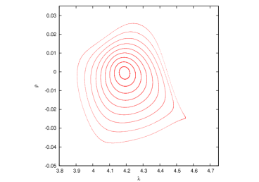
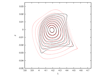
Figure 1: Left panel, in black surface of section obtained by a numerical integration of the CPRTBP. Middle panel, the surface of section for the same initial conditions computed with the normal form approximating the CPRTBP Hamiltonian. Right panel, the comparison between the two surfaces of section. In the three plots, $L_{4}$ is located at (${4\pi}/{3}$, $0$).

For the same initial conditions as before, we have integrated the orbits also according to the semi-analytical scheme (20), up to collect also 1000 points over the surface. This computations have been automatically made by a code written in C, in such a way to use the expansions of the normal form ${\cal Z}^{(R_{1},R_{2})}$ and the canonical transformation ${\cal C}^{(R_{1},R_{2})}$, which were preliminarly produced by using Mathematica. The truncations have been made according to the following values of the parameters ruling the extension of those expansions: $R_{1}=3$, $R_{2}=5$, $K=5$, $l_{max}=5$ and $s_{max}=3$. These values imply reasonable computing times. The results are expressed in the middle panel of Fig. 1. Finally, in the right panel, we show the comparison between the two surfaces of section. For all the orbits close to the equilibrium point $L_{4}\,$, the correlation is extremely good, thought the approximation fails on reproducing exactly the tadpole orbits far from $L_{4}\,$.

3 Optimal transfers by means of integrable aproximations

3.1 Baseline

Since the new normal form has $1$ d.o.f., it provides the integrable approximations of the motions of small bodies in the vicinity of the stable equilibrium points and suitable surfaces of section that are easy to compute. These tools can be used in many different studies. As explained in the Introduction, we focus in the design of maneuvres of small bodies (as spacecrafts or space debris) that are originally out of the stability region filled by tadpole orbits and we would like to situate into it. With such an aim, we design a method that allows to study the effectiveness of a set of impulses, done after considering a fixed initial position.

As outline of the algorithm, we have to

• choose a starting point $P_{s}$, which corresponds to the position of the body to transfer at $t=0$ and translate it to cartesian coordinates $P_{s}=\big{(}x_{0},y_{0},V_{x_{0}},V_{y_{0}}\big{)}$.

• give an impulse

  $$\Delta V_{x_{0}}=\|\Delta\mathbf{V}\|\cos\beta\qquad\Delta V_{y_{0}}=\|\Delta\mathbf{V}\|\sin\beta\ ,$$ (21)

  where $\|\Delta\mathbf{V}\|$ and $\beta$ are the modulus and direction of the impulse, respectively, in cartesian coordinates. This gives a new orbit, whose evolution in normalized variables can be computed with the integrable approximation of the Hamiltonian and checked in the surfaces of section.

• decide the acceptance or rejection of the impulse, according to whether it fulfills or not the conditions of the transfer.

As a matter of fact, this mechanism can be applied for a physically adequate range of moduli and directions and not one orbit by one, in order to speed up the computations.

3.2 Application and results

We apply the method described above to the case of the Earth-Moon system. As starting point $P_{s}\,$, we choose a position slightly outside the real stability region, estimated by numerical integrations of the full problem. $P_{s}$ is given by $\lambda=3.95$, $\rho=0$, $\xi=0.0885442$ and $\eta=0$. For the transfer orbits, we apply $10^{4}$ different impulses, for which $0\leq\|\Delta\mathbf{V}\|\leq 0.01\,$ and $0\leq\beta<2\pi\,$. Following §2.8 in [6], (1) and (19), we translate every orbit to normalized variables. In Fig. 2, we present the results of the translation of the new coordinates calculated after each impulse (for the first new point of the orbit on the surface of section) in the corresponding variables. The color scale represents the size of the impulse $\|\Delta\mathbf{V}\|$ in the left panel and its direction $\beta$ in the right panel. As expected, a stretching effect occurs while translating to the new system, and the impulses are more effective (i.e., same values imply a bigger difference with respect to the original point $P_{s}$) in some directions.

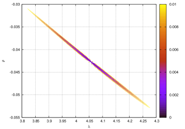
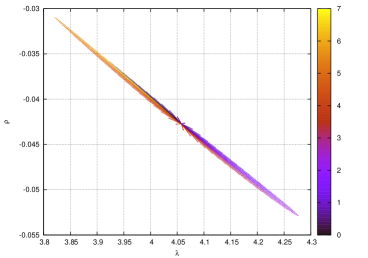
Figure 2: Color scheme for the initial conditions produced after applying the impulses. Left panel, new positions in ($\lambda$,$\rho$). The color scale represents the magnitude of the impulse $\|\Delta\mathbf{V}\|$. Right panel, same as before with color scale representing the direction of the impulse $\beta$.

In order to distinguish which impulses generate orbits that go deeper inside the stability region, we isolate the impulses pointing towards the inner part. We refine the values of the angles considered, taking $100$ equidistant values $\beta$, where $0.46\leq\beta\leq 0.86\,$. We integrate their evolution with respect to the normal form ${\cal Z}^{(5,3)}$ and we find the curves described by these orbits on the surface of section. In the averaged normal form, each of these curves depicts the area associated to one of the actions defining the 2-D torus that is invariant with respect to the motion. Since as closer the torus is to the equilibrium point $L_{4}\,$, as smaller this area is, we take as criterion for a good transfer a reduction of this value with respect to the initial one (Minimum Action criterion, since such an area corresponds to an action). In Fig. 3, we show the results of the computation of the area in two different color-scales. In the left panel, we can see for all the considered combinations of modulus $\|\Delta\mathbf{V}\|$ and angles $\beta$, the value of the area described by the transfered orbit. The lower border of the plot represents the orbits with $\|\Delta\mathbf{V}\|=0$, so their areas ($A_{0}$) are equal and can be used as reference value. In the right panel, only orbits corresponding to areas $\leq A_{0}$ are considered, the greater ones are fixed equal to $A_{0}\,$. This allows a better discrimination between all the orbits providing suitable impulses.

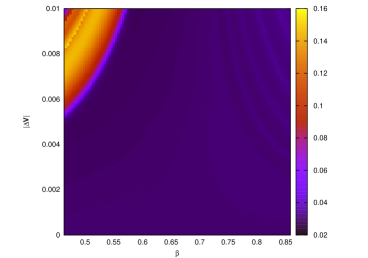
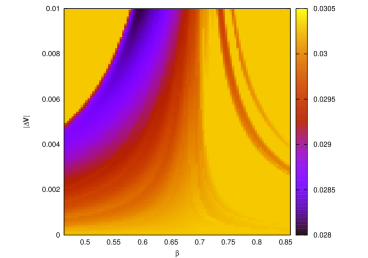
Figure 3: Left panel, values of the areas enclosed in the surface of section for every considered combination of $\|\Delta\mathbf{V}\|$ and $\beta$, the color scale represents the results of the calculations using the averaged normal form. Right panel, same as before where the computed areas are reported only if they are smaller than the value ($A_{0}$) corresponding to the original initial condition $P_{s}\,$.

Both plots shows that the selection of the angle for the impulse is not trivial, since small differences generate very different results. Consider, for instance, the impulses with $\beta=0.50$ and with $\beta=0.55\,$, for $\|\Delta\mathbf{V}\|>0.006$). The former give the best approach to the optimal transfer we look for, while the latter generate orbits which are actually further from $L_{4}$ than that related to the initial condition $P_{s}\,$. In general, since we take small values for the impulses, in the correct directions, bigger $\|\Delta\mathbf{V}\|$ implies smaller final areas. The best choices for the transfer correspond to the impulses for which $\beta\in[0.50\,,\,0.68]\,$, and suitable values for their sizes, following the darker stripes in Fig. 3.

4 Conclusions

In this work we explicitly construct an integrable normal form approximating the CPRTBP Hamiltonian. This is done by reformulating the approach described in [4] so as to use some more modern techniques, developed in the framework of the Hamiltonian perturbation theory and mainly based on the Lie series formalism. This allow us to design an algorithm that can be fully translated in programming codes. In particular, we produce a truncation of the normal form ${\cal Z}^{(5,3)}$, whose the expansion in (16) highlights that it is an average of the CPRTBP Hamiltonian with respect to the angle associated to its fast dynamics. The first results provided by this revisited approach are encouraging: in some suitable surface of sections our algorithm provides very good approximations of the tadpole orbits close enough to $L_{4}-L_{5}\,$. However, we are aware of the fact that the accuracy of our expansions must be strongly improved in order to face challenging concrete problems in a region far from those equilibrium points. In our opinion, the main constraint on the quality of our results is due to the truncations on the Fourier series in the slow angle $\lambda$. We think that this limitation can be removed, by representing the dependence on $\lambda$ in a suitable way, so as to avoid Fourier expansions. We plan to investigate such a new approach in the near future.

Furthermore, we show a first astrodynamical application starting from our calculation of the integrable normal form ${\cal Z}^{(5,3)}$, which approximates the CPRTBP Hamiltonian. We design an algorithm that allowed to compute optimal transfers between orbits in the neighborhood of the equilateral Lagrangian equilibrium points. We generate impulses in cartesian variables according to formula (21), on a grid of values for $\|\Delta\mathbf{V}\|$, the magnitude of the impulse, and $\beta$, the direction. For those, we are able to discriminate the suitable transfers, that imply a final orbit closer to the equilibrium point, according to a new criterion. Using our normal form as an approximation of the complete CPRTBP, we estimate the area enclosed by the final orbit, and minimizing this quantity, we select the best candidates for the transfer. A careful inspection of the plots shows that the best candidates are highly depending on the size of the impulse, and very sensitive to the changes on the angle $\beta$.

References

- [1] Arnold, V.I., Mathematical Methods of Classical Mechanics, 2-nd edition, Springer-Verlag, New York (1989).
- [2] Efthymiopoulos, C., “High order normal form stability estimates for co-orbital motion”, Cel. Mech. & Dyn. Astr, 117, 101–112 (2013).
- [3] Gabern, F., Jorba, A., and Locatelli, U., “On the construction of the Kolmogorov normal form for the Trojan asteroids”, Nonlinearity, 18, 1705–1734 (2005).
- [4] Garfinkel, B., “Theory of the Trojan asteroids, 1.”, Astronomical Journal, 82, 368–379 (1977).
- [5] Giorgilli, A., “Notes on exponential stability of Hamiltonian systems”, in Dynamical Systems, Part I: Hamiltonian systems and Celestial Mechanics, Pubblicazioni del Centro di Ricerca Matematica Ennio De Giorgi, 87–198 (2003).
- [6] Murray, C.D., and Dermott, S.F., Solar System Dynamics, Cambridge University Press, Cambridge (1999).
- [7] Nekhoroshev, N.N.: “Exponential estimates of the stability time of near–integrable Hamiltonian systems”, Russ. Math. Surveys, 32, 1–65 (1977).
- [8] Nekhoroshev, N.N.: “Exponential estimates of the stability time of near–integrable Hamiltonian systems, 2.”, Trudy Sem. Petrovs., 5, 5–50 (1979).
- [9] Perozzi, E., Marson, R., Teofilatto, P., Circi, C., and Di Salvo, A., “On the Accessibility of the Moon”, in Space Manifold Dynamics, E. Perozzi and S. Ferraz-Mello eds., Springer, 149–159 (2010).
- [10] Páez, R.I., “Exploring the Marginal Stability Region of the Tadpole Orbits for the Planar Circular Restricted Three–Body Problem: an Approach based on Normal Forms”, Internal Report within the Marie Curie ITN AstroNet-II, 1–39 (2013); available on request to the Author.