Abstract: In the framework of the ERTBP, we study an example of the influence of secondary resonances over the long term stability of Trojan motions. By the integration of ensembles of orbits, we find various types of chaotic diffusion, slow and fast. We show that the distribution of escape times is bi-modular, corresponding to two populations of short and long escape times. The objects with long escape times produce a power-law tail in the distribution.

1 Resonances

We study an example of mass parameter $\mu=0.0041$ and eccentricity $e^{\prime}=0.02$ of the primary in the framework of the ERTBP. Following Páez & Efthymiopoulos 2014 (hereafter, P&E14), we describe Trojan orbits in terms of modified Delaunay variables given by

$$x=\sqrt{a}-1,\quad y=\sqrt{a}\left(\sqrt{1-e^{2}}-1\right),\quad\Delta u=\lambda-\frac{\pi}{3}-u_{0},\quad\omega\leavevmode\nobreak\ \leavevmode\nobreak\ ,$$

where $a$, $e$, $\lambda$ and $\omega$ are the major semi-axis, eccentricity, mean longitude, and argument of the perihelion of the Trojan body, and $u_{0}$ is such that $\Delta u=0$ for the $1$:$1$ short period orbit at $L_{4}$.

In this problem, the secondary resonances (see P&E14) are of the form $m_{f}\omega_{f}+m_{s}\omega_{s}+m_{g}\omega_{g}=0$, involving the fast frequency $\omega_{f}$, the synodic frequency $\omega_{s}$ and the secular frequency $\omega_{g}$ of the Trojan body. Resonances are denoted below as [$m_{f}$:$m_{s}$:$m_{g}$]. The most important resonances, called the ’main’ secondary resonances, correspond to the condition $\omega_{f}-n\omega_{s}=0$ ([$1$:$-n$:$0$]). For $\mu=0.0041$, this corresponds to [$1$:$-6$:$0$].

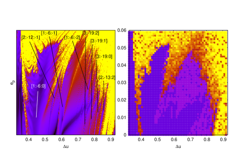
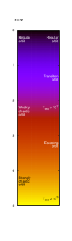
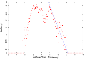
Figure 1: Left: FLI map for initial conditions described in the text where various secondary resonances are distinguished in the space of proper elements ($\Delta u$,$e_{p}$). Middle: Color distribution of escaping times for the same initial conditions (color scale indicated). Right: distribution of the escaping times of the orbits.

2 Diffusion and stability

Numerical experiments show that, for $e^{\prime}>0$, at least two different mechanisms of diffusion are present. Along non-overlapping resonances, a slow (and practically undetectable) Arnold-like diffusion (Arnold, 1964) takes place. On the other hand, for initial conditions along partly overlapping resonances, due to the phenomenon of pulsating separatrices (P&E14), we observe a faster ’modulational’ diffusion (Chirikov et al., 1985) leading to relatively fast escapes.

In order to distinguish which parts of the resonant web provide each behavior, we integrate 3600 initial conditions with $0.33\leq\Delta u\leq 0.93$ and $0\leq e_{p}\leq 0.06$, where $\Delta u$ (libration angle) and $e_{p}$ (proper eccentricity) are proper elements (see Efthymiopoulos and Páez, this volume). We visualize the resonance web by color maps of the Fast Lyapunov Indicator FLI (Froeschlé et al., 2000) of the orbits. The resonances are identified by Frequency Analysis (Laskar, 1990). We integrate all orbits up to $5$ different integration times along $10^{7}$ periods of the primaries. After each integration, the initial conditions are categorized as Regular (if $\Psi(t)<\log_{10}(\frac{N}{10})$, where $\Psi$ denotes the FLI value and $N$ is the total number of integration periods), Escaping (if the orbit undergoes a sudden jump in the numerical energy error greater than $10^{-3}$) or Transition (non Regular nor Escaping).

N. of periods	Regular Orb	Transition Orb	Escaping Orb
$10^{3}$	1220 ($33.8\%$)	2027 ($56.3\%$)	353 ($09.9\%$)
$10^{4}$	1263 ($35.0\%$)	1388 ($38.5\%$)	946 ($26.5\%$)
$10^{5}$	1296 ($36.0\%$)	966 ($26.8\%$)	1338 ($37.2\%$)
$10^{6}$	1299 ($36.1\%$)	699 ($19.4\%$)	1602 ($44.5\%$)
$10^{7}$	1309 ($36.3\%$)	603 ($16.8\%$)	1688 ($46.9\%$)

After $10^{7}$ periods, $46.9\%$ of the orbits have escaped. However, a significant portion ($16.8\%$) still remain trapped, despite having a high FLI value. Figure 1 resumes the results. The histogram in the right panel shows two distinct timescales. The first peak ($10^{3}$ periods), corresponds to fast escapes, and the second ($10^{5}$ periods), to slow escapes. When we compare the FLI map (left) with the color distribution of the escaping times (middle), we find that the majority of fast escaping orbits lay within the chaotic sea surrounding the secondary resonances. The thin chaotic layers delimiting the resonances provide both slowly escaping orbits and transition orbits (sticky set of initial conditions that do not escape after $10^{7}$ periods). For escaping orbits, beyond $t\sim 10^{5}$ periods, the distribution of the escape times is given by $P(t_{esc})\propto t_{esc}^{-\alpha},\,\alpha\approx 0.8$, while the sticky orbits exhibit features of ’stable chaos’ (Milani & Nobili, 1992), since their Lyapunov times are much shorter than $10^{7}$ periods.

Acknowledgements: R.I.P. was supported by the Astronet-II Training Network (PITN-GA-2011-289240). C.E. was supported by the Research Committee of the Academy of Athens (Grant 200/815).

References

- [1] Arnold, V.I. : Sov.Math.Dokr., 5, 581 (1964)
- [2] Chirikov, B.V., Lieberman, M.A., Shepelyansky, D.L., & Vivaldi, F.M.: Phys. D, 14, 289 (1985)
- [3] Froeschlé, C., Guzzo, M., & Lega, E.: Science, 289, 2108 (2000)
- [4] Laskar, J.: Icarus, 88, 266 (1990)
- [5] Milani, A., & Nobili, A.: Nature, 357, 569 (1992)
- [6] Páez, R.I., & Efthymiopoulos, C.: Cel.Mec.Dyn.Astron., 121, issue 2, 139 (2015)