First results and future prospects for dual-harmonic searches for gravitational waves from spinning neutron stars

Abstract

We investigate a method to incorporate signal models that allow an additional frequency harmonic in searches for gravitational waves from spinning neutron stars. We assume emission is given by the general triaxial non-aligned model of Jones, whose waveform under certain conditions reduces to that of a biaxial precessing star, or a simple rigidly rotating triaxial aligned star. The triaxial non-aligned and biaxial models can produce emission at both the star’s rotation frequency ($f$) and $2f$, whilst the latter only emits at $2f$. We have studied parameter estimation for signal models using both a set of physical source parameters, and a set of waveform parameters that remove a degeneracy. We have assessed the signal detection efficiency, and used Bayesian model selection to investigate how well we can distinguish between the three models. We found that for signal-to-noise ratios (SNRs) $\gtrsim 6$ there is no significant loss in efficiency if performing a search for a signal at $f$ and $2f$ when the source is only producing emission at $2f$. However, for sources with emission at both $f$ and $2f$ signals could be missed by a search only at $2f$. We also find that for a triaxial aligned source, the correct model is always favoured, but for a triaxial non-aligned source it can be hard to distinguish between the triaxial non-aligned model and the biaxial model, even at high SNR. Finally, we apply the method to a selection of known pulsars using data from the LIGO fifth science run. We give the first upper limits on gravitational wave amplitude at both $f$ and $2f$ and apply the model selection criteria on real data.

1 Introduction

Several searches have been performed for gravitational waves from known pulsars in data from the LIGO, GEO600 and Virgo gravitational wave detectors (Abbott et al., 2005, 2007, 2008, 2010; Abadie et al., 2011; Aasi et al., 2014). These rely on the known phase evolution of the pulsars from electromagnetic observations (e.g. Manchester et al., 2005) to allow long duration (of order a year) coherent searches for signals from them in gravitational wave data. Unfortunately no signal has yet been seen, but interesting upper limits on gravitational wave amplitude have been produced, and for two pulsars (the Crab and Vela pulsars) the “spin-down limit” has been beaten (Abbott et al., 2008; Abadie et al., 2011). One of the principal previous methods used for these searches (Dupuis & Woan, 2005) has focussed on parameter estimation and the setting of upper limits, but has not provided any measure of detection confidence.

Previous gravitational wave searches targeting known pulsars have assumed gravitational wave emission at a single frequency, taken to be twice (or very close to twice) the spin frequency. However, there are reasons to consider slightly more general waveforms. In this paper we consider the model proposed by Jones (2010), dealing with steadily rotating triaxial stars. Specifically, Jones (2010) considered a star containing a pinned superfluid. Such a star can rotate steadily about an axis that does not coincide with the principal axis of the solid crust, and will generically emit gravitational radiation at both the spin frequency $f$ and at $2f$. We term this the triaxial non-aligned case. This contrasts with the ‘standard’ scenario, considered in almost all gravitational wave searches to date, of rotation about a principal axis, which emits only at $2f$. We term this the triaxial aligned case, and it can be regarded as a special case of the triaxial non-aligned case. Another special case is that of a biaxial star, where two moments of inertia of the star are equal. The waveform in this case is identical to that of a biaxial precessing star of the sort considered by Zimmermann & Szedenits (1979), which also produces gravitational waves at two frequencies. However, precession generically results in a modulation in the electromagnetic signal produced by a pulsar (see e.g. Jones & Andersson, 2001), something that is not clearly observed in the pulsar population. In contrast, in the model of Jones (2010), there is emission at $f$ and $2f$ even in a steadily spinning star. The attraction of this model is that such emission, at both $f$ and $2f$, might be being produced by any of the known pulsars, without leaving any tell-tale signature in the radio pulsations. It is therefore clearly of interest to understand the issues that arise when carrying out gravitational wave searches for such double-component signals.

In this paper we study how different parameterisations of the model affect the estimation of signal parameters and the astrophysical information that can be extracted. We also discuss applying Bayesian model selection to assess the detection of signals from these sources and perform comparisons between the different signal models. A similar study has been performed by Bejger & Królak (2014) although there analysis was based on a maximum likelihood approach to parameter estimation. We use the methods we have developed to analyse data from LIGO’s fifth science run (S5), setting upper limits on the emission at both $f$ and $2f$ for 43 known pulsars.

The plan of this paper is as follows. In Section 2 we give a brief description of the neutron star model and waveform, confining the details to Appendix A. In Section 3 we describe the Bayesian methodology we employ. In Section 4 we briefly look at the shape of the parameter probability distributions for two different signal parameterisations. In Section 5 we show how these Bayesian methods can allow us to distinguish between the three different sorts of signals described above. In Section 6 we present the results from applying a search for gravitational wave emission at both $f$ and $2f$ in LIGO data. We summarise our findings in Section 7.

2 The model

In this Section we describe the physical model and gravitational wave emission from our triaxial star. In Section 2.1 we use the original parameterisation of Jones (2010), while in Section 2.2 we use an alternative simpler set of parameters, as described in Jones (2015). The ranges of the relevant parameters are given in Section 2.3, again based on the analysis of Jones (2015).

2.1 The signal written in terms of source parameters

Here we recap the physical model given in Jones (2010). The neutron star is triaxial, with a moment of inertia tensor whose principal components are $(I_{1},I_{2},I_{3})$. Because of superfluid pinning, it can rotate about an axis, fixed in the inertial frame, that does not coincide with any one of these principal axes. This gives rise to gravitational wave emission at both $f$ and $2f$. The signal in a detector at the rotation frequency ($f$) is (Jones, 2010, 2015)

$$h^{f}(t)= F_{+}(\psi,t)\sin{\iota}\cos{\iota}\Big{\{}I_{21}\sin{2\lambda}\sin{\theta}\cos{\phi(t)}+$$

$$(I_{21}\cos{}^{2}{\lambda}-I_{31})\sin{2\theta}\sin{\phi(t)}\Big{\}}$$

$$-F_{\times}(\psi,t)\sin{\iota}\Big{\{}(I_{21}\cos{}^{2}{\lambda}-I_{31})\sin{2\theta}\cos{\phi(t)}-$$

$$I_{21}\sin{2\lambda}\sin{\theta}\sin{\phi(t)}\Big{\}},$$ (1)

and the signal at twice the rotation frequency ($2f$) is

$$h^{2f}(t)= 2F_{+}(\psi,t)(1+\cos{}^{2}\iota)\Big{\{}\big{[}I_{21}(\sin{}^{2}\lambda-\cos{}^{2}\lambda\cos{}^{2}\theta)-$$

$$I_{31}\sin{}^{2}\theta\big{]}\cos{2\phi(t)}+I_{21}\sin{2\lambda}\cos{\theta}\sin{2\phi(t)}\Big{\}}$$

$$-4F_{\times}(\psi,t)\cos{\iota}\Big{\{}I_{21}\sin{2\lambda}\cos{\theta}\cos{2\phi(t)}-$$

$$\big{[}I_{21}(\sin{}^{2}\lambda-\cos{}^{2}\lambda\cos{}^{2}\theta)-I_{31}\sin{}^{2}\theta\big{]}\sin{2\phi(t)}\Big{\}}.$$ (2)

The polarisation factors $F_{+}$ and $F_{\times}$ depend upon the polarisation angle $\psi$ of the source. They also depend on the position of the source on the sky. We have not explicitly labelled this dependence as these parameters would be known for a targeted gravitational wave search. The angle $\iota$ is the inclination angle of the star’s spin vector with respect to the observer.

The evolution in phase $\phi(t)$ is generated by the rotation of the star, so that $\phi(t)=2\pi\int_{t_{0}}^{t}f(t^{\prime})\,\mathrm{d}t^{\prime}+\phi_{0}$ where $f(t)$ is the frequency evolution and $\phi_{0}$ the phase at $t_{0}$. In practice, for targeted gravitational wave searches, $f(t)$ will be a known function (known e.g. from radio pulsar observations), and so we will simply write

$$\phi(t)=\Omega t+\phi_{0},$$ (3)

treating $\Omega=2\pi f$ as a constant.

The constant angles $(\theta,\phi_{0},\lambda)$ are the Euler angles that specify the orientation of the star with respect to the inertial frame (at time $t_{0}$). Here we have used $\lambda$ to replace the ‘$\psi$’ parameter in Jones (2015) to avoid confusion with the standard use of $\psi$ for gravitational wave polarisation angle. The parameters $I_{21}$ and $I_{31}$ are measures of the asymmetry in the moment of inertia tensor, with factors of the angular spin frequency $\Omega$ and distance $r$ absorbed for convenience:

$$I_{21}\equiv\frac{\Omega^{2}(I_{2}-I_{1})}{r},\hskip 28.45274ptI_{31}\equiv\frac{\Omega^{2}(I_{3}-I_{1})}{r}.$$ (4)

Putting all of this together, and assuming that the sky position and spin frequency are already known, we have a set of seven source parameters:

$$\mn@boldsymbol{\theta}^{a}_{\rm source}=\{\iota,\psi,I_{21},I_{31},\theta,\phi_{0},\lambda\}.$$ (5)

We term this general case the triaxial non-aligned model of a spinning neutron star. There are two special cases that we will single out. The first is a triaxial star spinning about a principal axis. This can be obtained from Eqns  (2.1) and (2.1) by setting $\theta=0$; there is then emission only at $2f$. We term this the triaxial aligned case. The second special case is the biaxial case, where two of the principal components of the quadrupole moment tensor are equal. This can be found by setting $I_{21}=0$, and produces emission at both $f$ and $2f$. Note that, physically, this is slightly different from the relatively well-known precessional motion of a biaxial star (see e.g. Zimmermann & Szedenits, 1979; Jones & Andersson, 2002), as the latter has an additional slow rotation, superimposed about the symmetry axis. However, the time variation of the mass quadrupole, and therefore the corresponding gravitational waveforms, are identical in the two cases, so all of the discussion of the biaxial case in this paper applies also to the biaxial precession waveform. Nevertheless, it should be remembered that in the precession case, there can be modulation in the observed electromagnetic pulsation frequency, and the time average of this electromagnetic pulsation frequency can be offset from the gravitational wave frequency; see Jones & Andersson (2002) for a detailed discussion.

2.2 The signal written in terms of waveform parameters

As previously shown by one of us (Jones, 2015), and also explained in Bejger & Królak (2014), the physical source model, specified by the seven parameters of Eqn. (5), contains a degeneracy. If we instead express the model as complex harmonic amplitudes we find that Eqns. (2.1) and (2.1) can be rewritten as

$$h^{f}(t)= -\frac{1}{2}F_{+}(\psi,t)C_{21}\sin{\iota}\cos{\iota}\cos{\left(\phi(t)+\Phi_{21}^{C}\right)}-$$

$$\frac{1}{2}F_{\times}(\psi,t)C_{21}\sin{\iota}\sin{\left(\phi(t)+\Phi_{21}^{C}\right)},$$ (6)

and

$$h^{2f}(t)= -F_{+}(\psi,t)C_{22}[1+\cos{}^{2}\iota]\cos{\left(2\phi(t)+\Phi_{22}^{C}\right)}-$$

$$2F_{\times}(\psi,t)C_{22}\cos{\iota}\sin{\left(2\phi(t)+\Phi_{22}^{C}\right)}.$$ (7)

There now appear two amplitude-like parameters $C_{21}$ and $C_{22}$ with corresponding phase parameters $\Phi^{\rm C}_{21}$ and $\Phi^{\rm C}_{22}$. Assuming that the sky location and spin frequency are known, we can identify a set of $6$ waveform parameters, one fewer than in the case of the source parameters:

$$\mn@boldsymbol{\theta}^{a}_{\rm waveform}=\{\iota,\psi,C_{21},C_{22},\Phi^{\rm C}_{21},\Phi^{\rm C}_{22}\}.$$ (8)

When expressed in terms of these waveform parameters, a problematic degeneracy is removed, as we will illustrate in Section 4 below. Comparing with the source parameters of Eqn. (5), we see that the two angles $(\iota,\psi)$ giving the orientation of the star’s spin axis relative to the observer are common to both sets. There is in fact a rather complicated algebraic relationship between the five remaining source parameters $(I_{21},I_{31},\theta,\phi_{0},\lambda)$ and the four remaining waveform parameters $(C_{21},C_{22},\Phi^{\rm C}_{21},\Phi^{\rm C}_{22})$. This relation is derived in Jones (2015), and reproduced in Appendix A, where we also summarise the form that the waveform parameterisation takes when specialised to the triaxial aligned and biaxial cases. As shown in Jones (2015), the parameters $C_{21}$ and $C_{22}$ are basically the (moduli) of the (complex) mass quadrupole scalars that describe the quadrupolar component of the mass distribution of the rotating star, with a factor of order $\Omega^{2}/r$ absorbed for simplicity. (Note that in Jones (2015) these quantities are denoted by $\tilde{C}_{21},\tilde{C}_{22}$).

Note that in this analysis we are assuming a search for gravitational wave signals from known pulsars, or sources where a significant gravitational wave signal has already been found. This means that, rather than using the waveforms as written in Eqns (2.1–2.1), or Eqns (6–7), we can remove the oscillations that take place at the relatively high frequencies $f$ and $2f$, using the heterodyne method of Dupuis & Woan (2005) to give instead a pair of narrow-band complex times series. We do this by using the known phase evolution of the signal $\phi(t)$, multiplying by $\mathrm{e}^{-i\phi(t)}$ for the $f$-band and $\mathrm{e}^{-\mathrm{i}2\phi(t)}$ for the $2f$-band. This heterodyning, and subsequent low-pass filtering, leaves a signal model for the $f$ and $2f$ streams of

$$h_{f}(t)=-\frac{C_{21}}{4}F_{+}(\psi,t)\sin{\iota}\cos{\iota}\mathrm{e}^{\mathrm{i}\Phi_{21}^{C}}+i\frac{C_{21}}{4}F_{\times}(\psi,t)\sin{\iota}\mathrm{e}^{\mathrm{i}\Phi_{21}^{C}}$$ (9)

and

$$h_{2f}(t)=-\frac{C_{22}}{2}F_{+}(\psi,t)[1+\cos{}^{2}\iota]\mathrm{e}^{\mathrm{i}\Phi_{22}^{C}}+iC_{22}F_{\times}(\psi,t)\cos{\iota}\mathrm{e}^{\mathrm{i}\Phi_{22}^{C}}$$ (10)

when written in terms of the waveform parameters. A similar heterodyning can be applied to the waveform when written in terms of the source parameters (see Gill, 2012).

2.3 Parameter ranges

In order to carry out our analyses, we need to choose sensible ranges in both the source and waveform parameters, for each of the triaxial aligned, biaxial and triaxial non-aligned models. The choice of ranges in these parameters turns out to be rather subtle, and is described in detail in Jones (2015). Basically, the source parameterisation, and, to a lesser extent, the waveform parameterisation, contain various discrete degeneracies, where changes in some combination of angle and/or amplitude parameters leaves the detected waveform $h(t)$ invariant. This allows the ranges in these parameters to be reduced as compared to one’s initial expectations, with there being several options as to how the parameter space is reduced. The choices given in Tables 1 and 2 represent one of several possibilities (see Jones, 2015), and are the ranges we have used for the subsequent analyses presented in this paper. Any point in these ranges can be mapped into another part of the full parameter range that gives an identical waveform through the transformations given in Jones (2015). This enables signal parameter estimation and evidence evaluation to be performed using this minimal range, but for posteriors to then be mapped into the full range, if so desired.

Table 1: Parameter ranges for the waveform parameters for the three signal models.

	Models
	Triaxial aligned	Biaxial	Triaxial non-aligned
$C_{21}$	—	$-C_{21}^{\rm max},C_{21}^{\rm max}$	$0,C_{21}^{\rm max}$
$C_{22}$	$0,C_{22}^{\rm max}$	$-C_{22}^{\rm max},C_{22}^{\rm max}$	$0,C_{22}^{\rm max}$
$\Phi_{21}^{C}$ (rads)	—	$0,2\pi$	$0,2\pi$
$\Phi_{22}^{C}$ (rads)	$0,2\pi$	$2\Phi_{21}^{C}$	$0,2\pi$
$\psi$ (rads)	$0,\pi/2$	$0,\pi/2$	$0,\pi/2$
$\cos{\iota}$	$-1,1$	$-1,1$	$-1,1$

Table 2: Parameter ranges for the source parameters for the three signal models.

	Models
	Triaxial aligned	Biaxial	Triaxial non-aligned
$I_{31}$	—	$0,I_{31}^{\rm max}$	$I_{21},I_{31}^{\rm max}$
$I_{21}$	$0,I_{21}^{\rm max}$	—	$0,I_{21}^{\rm max}$
$\phi_{0}$ (rads)	$0,\pi$	$0,2\pi$	$0,2\pi$
$\lambda$ (rads)	—	—	$0,\pi$
$\cos{\theta}$	1	$0,1$	$0,1$
$\psi$ (rads)	$0,\pi/2$	$0,\pi$	$0,\pi/2$
$\cos{\iota}$	$-1,1$	$-1,1$	$-1,1$

3 Bayesian methodology

For this analysis we want to be able to compute probability distributions for source and waveform parameters, and also to compare models (noise-only verses triaxial non-aligned verses biaxial verses triaxial aligned). In Bayesian methodology the standard way to compute probability distributions for unknown parameters is make use of Bayes theorem for the posterior probability distribution

$$p(\mn@boldsymbol{\theta}|d,M,I)=\frac{p(d|\mn@boldsymbol{\theta},M,I)p(\mn@boldsymbol{\theta}|M,I)}{p(d|M,I)},$$ (11)

where $p(d|\mn@boldsymbol{\theta},M,I)$ is the likelihood of the data $d$ given model $M$ and background information $I$, with a set of parameters $\mn@boldsymbol{\theta}$, $p(\mn@boldsymbol{\theta}|M,I)$ is the prior on the parameters, and $p(d|M,I)$ is the evidence, or marginal likelihood (in this paper we will use the term evidence throughout for consistency), of the data given the model. The evidence is the factor that normalises the posterior probability density. It is given by

$$p(d|M,I)=\int_{\mn@boldsymbol{\theta}}p(d|\mn@boldsymbol{\theta},M,I)p(\mn@boldsymbol{\theta}|M,I)\mathrm{d}\mn@boldsymbol{\theta}.$$ (12)

To compare models, we can calculate the Bayes factor, or odds ratio, between competing models. To this end, note that for any model we can calculate its posterior probability as

$$p(M|d,I)=\frac{p(d|M,I)p(M|I)}{p(d|I)}.$$ (13)

It is hard (maybe impossible) to calculate the normalisation factor $p(d|I)$ as you have to know all alternative models and marginalise over them, but we can still compare posterior probabilities between models provided they use the same data. We can compute the Bayes factor, or odds ratio $\mathcal{O}$ (which we will use from here onwards) between two models, as e.g.

$$\mathcal{O}_{12}=\frac{p(M_{1}|d,I)}{p(M_{2}|d,I)}=\frac{p(d|M_{1},I)}{p(d|M_{2},I)}\frac{p(M_{1}|I)}{p(M_{2}|I)}.$$ (14)

Note that the normalising factor $p(d|I)$ has canceled out. If there is no known prior preference between the two models then the ratio $p(M_{1}|I)/p(M_{2}|I)$, the ratio of the prior odds between each model, can be set equal to unity. In this case, the odds ratio is just the ratio between the evidences, given by Eqn. (12), of the two models. We will adopt this viewpoint here, so all odds ratios will be calculated as the ratio of evidences.

In the analyses performed in Sections 4 and 5 the likelihood function $p(d|\mn@boldsymbol{\theta},M,I)$ we use is the Student’s $t$ likelihood given in Dupuis & Woan (2005). This likelihood assumes that the noise in the data is stationary (over the defined length of time) and Gaussian, but with an unknown noise standard deviation that has been analytically marginalised out. However, for the analysis of real data in Section 6 we have instead estimated the noise level for each data point and therefore use a Gaussian likelihood function in that section. The reason for this difference in likelihood function is that for real data it is more efficient to produce our processed data set at a lower sample rate and with the noise already estimated, which makes the Gaussian likelihood more appropriate. However, for large numbers of data points the two likelihoods will be very similar.

3.1 Priors

To compute evidences and posterior probability distributions we must also explicitly define our prior probability distributions. For the azimuthal-type angular parameters, and uniform in the cosine of the polar-type angular parameters, the least informative prior is a uniform prior defined within their allowed ranges. So, given the ranges in Tables 1 and 2, the prior on the angles in the waveform parameterisation, assuming the triaxial non-aligned model, are

$$p(\Phi_{21}^{C},\Phi_{22}^{C},\psi,\cos{\iota}|M,I)=\begin{cases}\mathrm{const.}&\parbox[t]{86.72267pt}{if $0\leq\Phi_{21}^{C}\leq 2\pi$ \\ and $0\leq\Phi_{22}^{C}\leq 2\pi$ \\ and $0\leq\psi\leq\pi/2$ \\ and $-1\leq\cos{\iota}\leq 1$; }\\ 0&\textrm{otherwise,}\end{cases}$$ (15)

whilst in the source parameterisation, assuming the triaxial non-aligned model, it is

$$p(\phi_{0},\lambda,\psi,\cos{\theta},\cos{\iota}|M,I)=\begin{cases}\mathrm{const.}&\parbox[t]{86.72267pt}{if $0\leq\phi_{0}\leq 2\pi$\\ and $0\leq\lambda\leq\pi$ \\ and $0\leq\cos{\theta}\leq 1$ \\ and $0\leq\psi\leq\pi/2$ \\ and $-1\leq\cos{\iota}\leq 1$; }\\ 0&\textrm{otherwise.}\end{cases}$$ (16)

Equivalents of these priors for the required parameters are used in the triaxial aligned and biaxial cases.

We will use priors on the amplitude parameters that are uniform within a range defined by the limits in Tables 1 and 2. These limits on the priors vary for the different model types, as described in Jones (2015). For the waveform parameterisation in the triaxial non-aligned case our prior is

$$p(C_{21},C_{22}|M,I)=\begin{cases}\mathrm{const.}&\parbox[t]{130.08731pt}{if $0\leq C_{21}\leq C_{21}^{\rm max}$ \\ and $0\leq C_{22}\leq C_{22}^{\rm max}$;}\\ 0&\textrm{otherwise.}\end{cases}$$ (17)

but for the biaxial case it is

$$p(C_{21},C_{22}|M,I)=\begin{cases}\mathrm{const.}&\parbox[t]{130.08731pt}{if $-C_{21}^{\rm max}\leq C_{21}\leq C_{21}^{\rm max}$\\ and $-C_{22}^{\rm max}\leq C_{22}\leq C_{22}^{\rm max}$\\ and $C_{22}/C_{21}\geq 0$;}\\ 0&\textrm{otherwise.}\end{cases}$$ (18)

For the source parameterisation in the triaxial non-aligned case we choose to use a prior on the amplitudes given by

$$p(I_{31},I_{21}|M,I)=\begin{cases}\mathrm{const.}&\parbox[t]{130.08731pt}{if $0\leq I_{31}\leq I_{31}^{\rm max}$ \\ and $0\leq I_{21}\leq I_{21}^{\rm max}$\\ and $I_{31}>I_{21}$;}\\ 0&\textrm{otherwise.}\end{cases}$$ (19)

These priors on the amplitude parameters are uniform largely for convenience and simplicity rather than through a physical motivation. This is consistent with the uniform priors traditionally used in searches for gravitational waves from known pulsars, where uniform amplitude priors play a role of allowing a relatively high upper limit to be set by the likelihood, consistent with the data. However, when evaluating evidences a choice of uniform prior does have an influence, as doubling an allowed parameter range doubles the effective prior volume. However, we limit the effect of this in our analysis by assessing the distribution of odds ratios between signal and noise models empirically and basing thresholds on that empirical distribution. Additionally some of the influences of the size of prior volume cancel when comparing signal models. It is worthwhile noting that evidence values produced using the minimal parameter ranges given in Tables 1 and 2 are equivalent to those that would be produced using the full parameter space (or, e.g. just doubling the $\psi$ ranges). This is because the likelihood volume within the minimal range is exactly reproduced in each of the equivalent volumes within the total physical range, along with the prior volume increasing by the same factor. So, the increase in likelihood volume and prior volume cancel out.

3.2 Nested sampling

To calculate odds ratios we need to evaluate the evidence for each model, and Eqn. (12) shows this to involve multi-dimensional integrals. For some parameters, or likelihoods, the integral may be analytic, or for low numbers of dimensions it may be possible to evaluate it on a grid, but more generally, efficient numerical integration techniques must be applied. Here we use the nested sampling algorithm of Skilling (2006), in particular the implementation of it based on that developed by Veitch & Vecchio (2010) and available in the LALInference software library (Veitch et al., 2015). Nested sampling attempts to simplify Eqn. (12) into a one-dimensional integral that can be easily numerically calculated. It samples a number of live points from the prior parameter volume, calculates the likelihood at each point, finds the minimum likelihood $L_{\rm min}$ point to add to the evidence integral, and then samples a new point with a higher likelihood than $L_{\rm min}$. This process is repeated until the integral is computed to sufficient accuracy.

The analysis methods and models we have used have been incorporated into a code called lalapps_pulsar_parameter_estimation_nested, which is freely available in the LALSuite software repository.

4 Waveform versus source parameters

It is useful to look at some plots that illustrate the very different nature of the waveform and source parameters. To do so, we can make use of the samples produced during nested sampling, by probabilistically drawing a subset that represent the posterior probability distributions of the model parameters, using either the waveform or source parameters. The distribution of samples for an individual parameter (or subset of parameters) represent the posterior probability for that parameter marginalised over all other parameters. This amounts to integrating Eqn. (11) over the prior ranges given in Tables 1 and 2 for the required parameter(s). In Figs. 1 and 2 the one-and-two dimensional posterior parameter distributions are shown for the triaxial non-aligned model for an almost linearly polarised signal ($\cos{\iota}\approx 0$) with an SNR of 20, when recovered using the waveform and source parameters respectively. Equivalent plots for an almost fully circularly polarised signal ($|\cos{\iota}|\approx 1$) are shown in Figs. 3 and 4. We present results for these two extremes in inclination angle to give the reader an idea of the range of different posterior probability distributions than can be obtained.

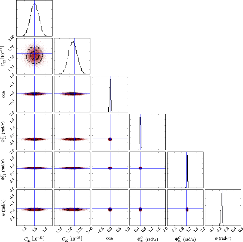
Figure 1: Marginalised posterior probability distribution plots of waveform parameters for an almost fully linearly polarised ($\cos{\iota}\approx 0$) signal with an SNR of 20 covering the minimal parameter ranges of Table 1. The cross-hairs show the true parameters of the simulated signal. All posterior plots have been produced with a modified version of the triangle.py python package (Foreman-Mackey et al., 2014).

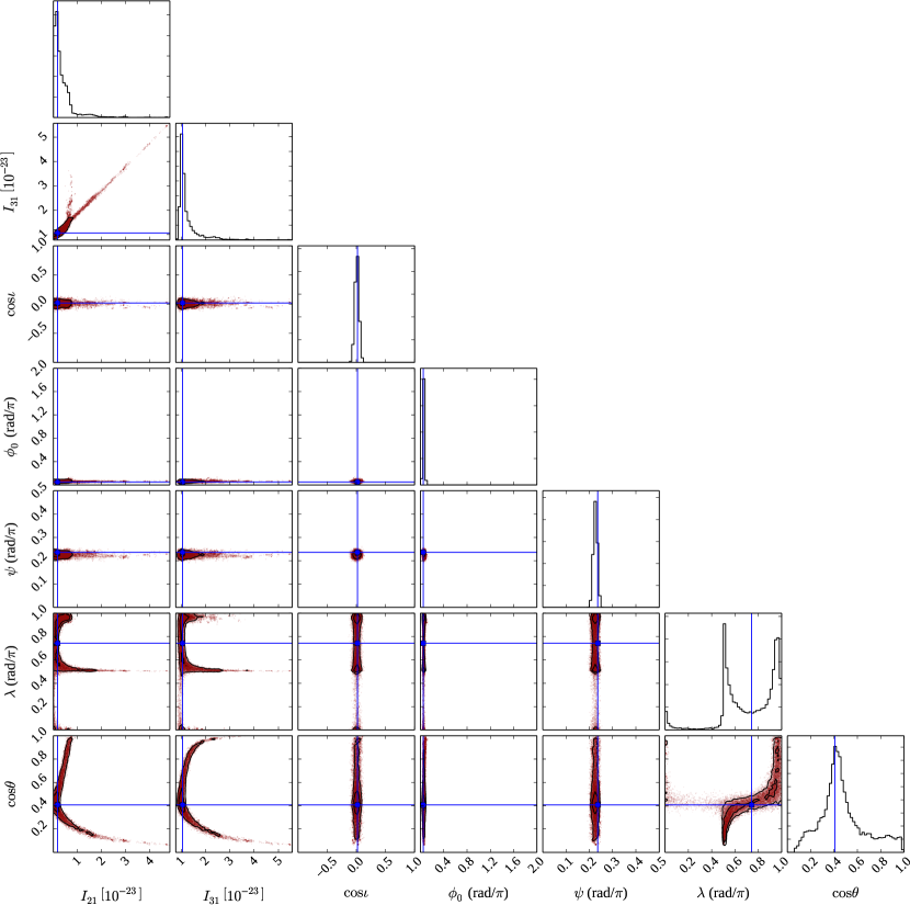
Figure 2: Marginalised posterior probability distribution plots of source parameters for an almost fully linearly polarised ($\cos{\iota}\approx 0$) signal with an SNR of 20 (the same signal as used in Fig. 1) covering the minimal parameter ranges of Table 2. The cross-hairs show the true parameters of the simulated signal.

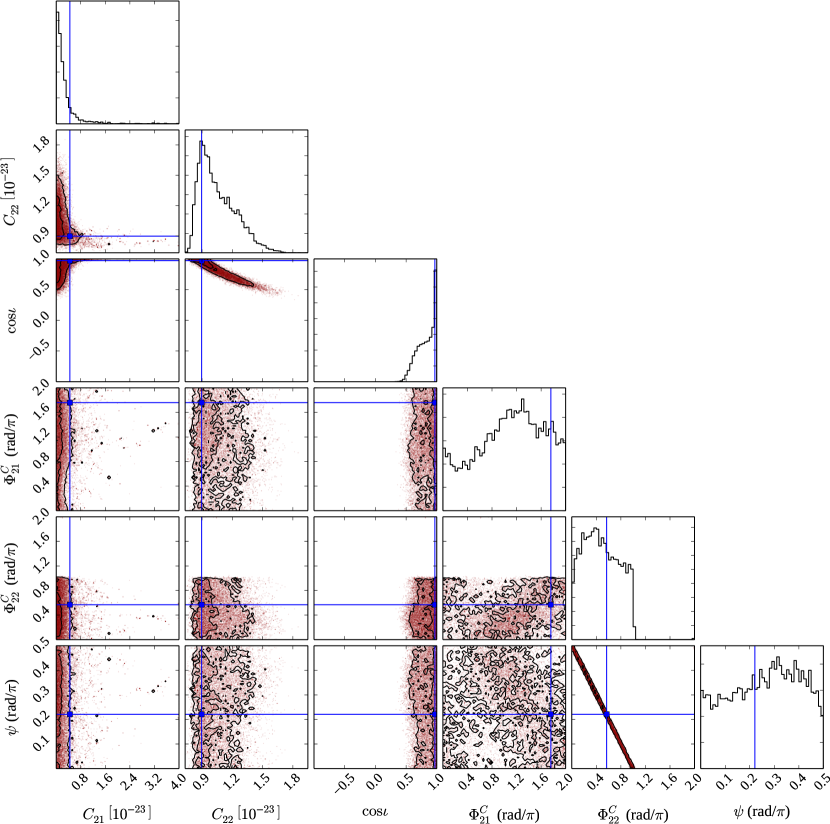
Figure 3: Marginalised posterior probability distribution plots of waveform parameters for an almost fully circularly polarised ($\cos{\iota}\approx 1$) signal with an SNR of 20 covering the minimal parameter ranges of Table 1. The cross-hairs show the true parameters of the simulated signal.

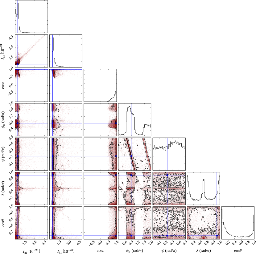
Figure 4: Marginalised posterior probability distribution plots of source parameters for an almost fully circularly polarised ($\cos{\iota}\approx 1$) signal with an SNR of 20 (the same signal as used in Fig. 3) covering the minimal parameter ranges of Table 2. The cross-hairs show the true parameters of the simulated signal.

From Figs. 1 and 3 it can be seen that the waveform parameters show a rather simple uni-modal probability distribution. This is especially evident for the close-to-linearly-polarised signal, which shows the posteriors to be largely uncorrelated and Gaussian in appearance; as has been seen in previous triaxial aligned analyses, the extraction of parameters for circular polarisations is slightly more difficult, due to increased correlations between the parameters (Pitkin, 2011). In contrast, the probability distributions in the source parameter space, shown in Figs. 2 and 4, show a large amount of structure (as originally observed in Gill, 2012). As described in Appendix A, the five source parameters $(I_{21},I_{31},\theta,\phi_{0},\lambda)$ can be related to the four waveform parameters $(C_{21},\Phi^{\rm C}_{21},C_{22},\Phi^{\rm C}_{22})$. This leads to the source parameters forming a highly degenerate and curved tube-like structure, rather than the much simpler form of the waveform parameters. The full complexity of this tube-like structure is probably being somewhat masked by our choice to only show its projected marginalisations in two dimensions.

We note that non-negligible probabilities exist out to large values if $I_{21}\approx I_{31}$, due to degeneracies with other parameters. For example, in Fig. 4, $I_{21}$ and $I_{31}$ are truncated to show the bulk of the posterior, but would otherwise show a long tail along the diagonal of the $I_{21}$ versus $I_{31}$ joint posterior plot. This long tail in $I_{21}$ and $I_{31}$ is particularly prominent given our choice of a uniform prior in the amplitude parameters. If we had used a prior uniform in the logarithm of the amplitude parameters then this tail would be greatly suppressed.

Clearly, it will be much simpler to work with the waveform parameters rather than source parameters. There is also the issue of computational speed. For a stochastic sampling technique such as nested sampling, the efficiency of the algorithm is greatly increased if new samples can be drawn from a distribution that closely matches the actual likelihood distribution. If the true distribution is smoothly varying, uni-modal, and relatively unstructured then it can generally be well approximated by a multivariate Gaussian. However, for more complex distributions such an approximation becomes invalid.

Indeed, comparisons in which the analysis code has been run on the same data, but using the waveform and source parameter spaces, show that to produce a similar number of posterior samples the former runs $\mathchar 21016\relax 1.6$ times faster than the latter in the case of no signal, and $\mathchar 21016\relax 1.8$ times faster for a signal with an SNR of $\mathchar 21016\relax 20$. This clearly shows the problems caused when sampling from likelihood functions with complex structure.

We can therefore see that working with the waveform model rather than the source model is simpler, both in terms of the dimensionality of the parameter space and the shape of the likelihood function, and the required computations are faster in the waveform case. For these reasons, in the model comparisons that follow in Section 5, we will work exclusively in terms of the waveform parameters.

4.1 Parameter space mapping

In the calculations described above, we have used ranges in the parameters that were as small as possible, i.e. we used the smallest possible sets such that one could be sure that if a triaxial non-aligned signal were present in the data, parameters could be found that matched the signal; see Jones (2015) for details. However, in the event of a detection, other parameters can be found that match the signal, in a way described using the transformations given in Jones (2015). Some of these other parameter sets correspond to physically distinct stars. For instance, if one finds a signal with a polarisation angle $\psi$, there will exist three other solutions with $\psi$ values that differ by successive additions of $\pi/2$, and having different values for some other the other parameters; this degeneracy can only be broken if additional (probably electromagnetic) information is available. There will also be other parameter sets that correspond to exactly the same physical star, and differ only in a trivial way, relating to how one chooses to label the three Cartesian axes that one lays down on the spinning triaxial body. It is instructive to fill out the full parameter space, to make clear that these degeneracies exist, and test the transformation rules given in Jones (2015).

In the case of the waveform model, we need only enlarge the range covered by the polarisation angle $\psi$, whose minimal range was $\psi\in[0,\pi/2]$, and so covered one quarter of the full range $\psi\in[0,2\pi]$ that $\psi$. So, to construct posteriors in the full range we can randomly split the posterior samples into quarters, and each successive quarter can be mapped into the adjacent parameter volume by successive application of the transformations given in the Appendix of Jones (2015)

$$\psi \rightarrow\psi+\pi/2,$$

$$\Phi_{21}^{C} \rightarrow\Phi_{21}^{C}+\pi,$$

$$\Phi_{22}^{C} \rightarrow\Phi_{22}^{C}+\pi.$$ (20)

For the source model the restricted range only covers a sixteenth of the full range (where $\cos{\theta}\in[-1,1]$, $\psi\in[0,2\pi]$ and $\lambda\in[0,2\pi]$). This means that the posterior samples have to be split between the sixteen volumes and more complex transforms used to map them as given in Jones (2015). If one wishes to map out this full parameter space, considerable care has to be taken when carrying out the transformations, particularly when selecting the correct roots of inverse trigonometric functions. For this reason, we give in Appendix B, a outline of the procedure used here, written as a simple pseudo-code.

The full posterior plots for the linearly polarised signal used in Figs. 1 and 2, based on this mapping of posterior samples are shown in Figs. 5 and 6. In the waveform parameterisation shown in Fig. 5, whilst the amplitude parameters and inclination can be unambiguously recovered, it is impossible through the gravitational wave signal alone to be able to distinguish the combination of initial phases and polarisation angle between the four distinct modes. In the source parameterisation things become even more complex. Whilst $I_{31}$ and $\cos{\iota}$ can be reasonably well determined the other parameters suffer from strong degeneracies. In particular there are always combinations of parameters that allow $I_{21}$ to be close to zero or large, which means that it may only be possible to ever set upper limits on this parameter, even in the event of a detection. This implies that for the triaxial aligned model precise determination of the individual physical parameters will not be possible even for high SNR sources. Only some highly correlated combination of parameters will be precisely determined.

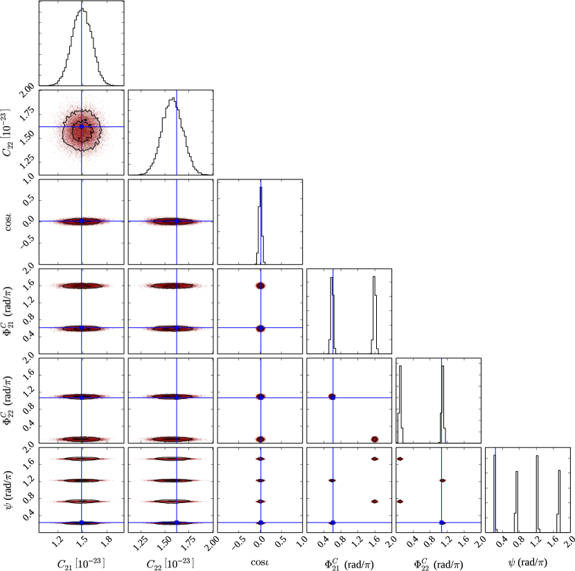
Figure 5: Marginalised posterior probability distribution plots of waveform parameters for the same signal as used in Fig. 1, but covering the full physical parameter ranges. The cross-hairs show the true parameters of the simulated signal.

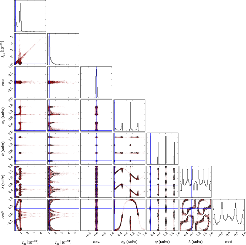
Figure 6: Marginalised posterior probability distribution plots of source parameters for the same signal as used in Fig. 1, but covering the full physical parameter ranges. The cross-hairs show the true parameters of the simulated signal.

The complex degeneracies of the posteriors for the source parameters show that trying to estimate parameter uncertainties using the Gaussian approximation of the Fisher matrix would most likely lead to highly biased results even at high SNRs. However, the waveform parameterisation looks to be far more amenable to estimation using the Fisher matrix (as is done in Bejger & Królak, 2014), provided that the minimal parameter space is used and the multi-modal degeneracies in the full parameter ranges are subsequently accounted for.

5 Model selection

In this section we use simulations of signals and noise to evaluate how well we can distinguish between noise-only data, and data containing a signal of the form of one of our three models (triaxial non-aligned, triaxial aligned, or biaxial). In all our simulations we have adopted a noise level for the $f$ and $2f$ data streams based on the initial LIGO design sensitivity for the 4 km LIGO Hanford Observatory (H1), i.e. the noise level is not equal between data streams and signal-to-noise ratios will be affected not just by the signal amplitude, but by their frequency. All simulations assume one day of heterodyned data sampled at a rate of one sample per minute, as has been standard in previous searches (Dupuis & Woan, 2005) and that the evidence evaluation uses a Student’s $t$ likelihood function. For the advanced detectors the sensitivity curve shapes will be similar, but with the low-frequency edge being pushed to lower frequencies. Note that in all of our analyses, we assume that the signal phase evolution is tracked exactly, so that the frequency $f$ is a known parameter.

Also in this section we will often refer loosely to the natural logarithm of the odds ratio, $\ln{\mathcal{O}}$, as the ‘odds ratio’. This number has the convenience of being far more robust against issues of numerical precision when dealing with very large or small likelihood values.

5.1 Noise-only simulations

The odds ratio itself tells you how much one model is favoured over another, but computed odds ratios will be numerically different for different noise realisations. Jeffreys (1998) gives a rule-of-thumb table for assessing the significance of odds ratios, however this can also be approached empirically by using simulations to determine their distribution over realisations. In particular, by assessing the odds ratios empirically we can alleviate the effect of our large prior amplitude volume in shifting the distribution of odds ratios towards low values even when signals could potentially be seen. We will therefore follow this second path. The dependence of the odds ratios we calculate on the prior volume of the amplitude parameters probably shows that our choice of amplitude priors (uniform up to some maximum, and zero above the maximum) could be improved upon. One alternative option is a prior that is uniform up to a lower maximum value and then uniform in the logarithm of amplitude for larger values. However, the simple choice we have made has the advantage that the same prior can be used for all sources, no matter where they sit within the detector’s sensitivity curve, with the knowledge that the prior will easily bound the bulk of the likelihood in all cases.

For our noise-only analysis we ran 2 000 simulations, with $f$ drawn from a uniform distribution between 50 and 700 Hz, and the $f$ and $2f$ data streams generated by drawing the real and imaginary components from Gaussian distributions with zero mean and a variance set by the expected H1 noise at the given frequency. For each simulation a random sky location was chosen, generated from a uniform distribution on the sky, as this determines the antenna pattern functions $F_{+}$ and $F_{\times}$ of Eqns (9) and (10). Note that, for the reasons outlined previously, when calculating odds ratios, we used signals written in terms of the waveform parameters rather than source parameters. For each simulation the odds ratios of evidence for each model versus that for Gaussian noise have been calculated using nested sampling, and the cumulative probability distributions of all these values are shown in Fig. 7. Note that for the triaxial aligned model only the $2f$ data stream was used.

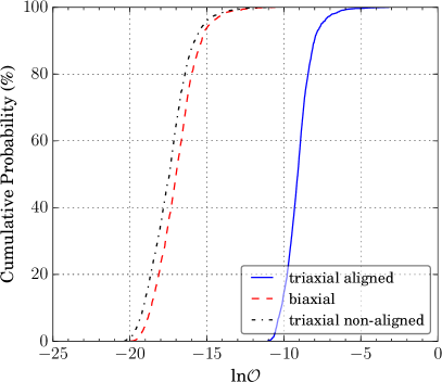
Figure 7: The cumulative probability distribution of odds ratios comparing the three signal models to Gaussian noise for data containing only noise.

Fig. 7 has three notable features. First, we see that the odds ratio ($\mathrm{e}^{\ln{\mathcal{O}}}$) for all three signal models is, for a large fraction of the simulations, small, confirming that noise-only data is normally found to be more consistent with noise than with a signal, as expected. Second, for a given cumulative probability, the odds ratios for the biaxial and triaxial non-aligned models are much smaller than for the triaxial aligned model. There are two related explanations for this: it is intrinsically less likely for noise to conspire to imitate a signal with components at both $f$ and $2f$, as this would require the noise to produce signal-like disturbances at the two widely-separated frequencies, with correlated properties (e.g. with consistent values for the parameters $\iota$ and $\psi$); and, there will be an Occam factor at play, such that in the absence of any evidence for a particular signal the simpler triaxial aligned model, which has fewer parameters and a correspondingly smaller prior volume than the biaxial and triaxial non-aligned models, will be favoured. In particular the large extra prior volume added by the extra amplitude parameter in the triaxial non-aligned and biaxial models play the predominant role in the shift between the odds ratio distributions. Third, the curves show that the biaxial model is slightly favoured over the triaxial non-aligned model. This again can be accounted for through the Occam factor, due to the additional parameter, and therefore prior volume, required for the triaxial non-aligned model over the biaxial model.

From these distributions we can set an odds ratio threshold at which we favour one model over noise at a given false alarm probability. If we choose a false alarm probability of 1% we find threshold odds ratios for each model versus Gaussian noise alone are $-6.3$, $-13.0$, and $-13.5$ for the triaxial aligned, biaxial and triaxial non-aligned cases respectively. We will use these thresholds for calculating detection efficiencies below. However, it is worth noting that analyses of data of different lengths of time, and/or combining additional detectors, would produce different values for the odds ratios. This means that a threshold needs to be calculated for a specific analysis and that the values above are only relevant if using one day of LIGO H1 data sampled at a rate of once per minute. A different threshold would be required for the analysis of real LIGO data presented in Section 6, and indeed in Section 6.1 we demonstrate a different, but related, assessment of detection significance. It is also worth noting that these simulations have used Gaussian noise, whereas the distribution of odds ratios for real data would most likely be different.

5.2 Signal simulations

To assess detection efficiencies for signals described by the three different models we have generated simulations including these signals. In all three cases we drew the signal sky positions from a uniform distribution on the sky, and chose amplitude parameters to give a uniform SNR distribution between $0$ and $20$. We chose the distribution of angular parameters to be uniform within the prior ranges given in Table 2. In the triaxial non-aligned case we drew values from the source parameters, with $I_{21}$ drawn from a uniform distribution between zero and an upper range, whilst for each $I_{21}$ value $I_{31}$ was drawn from a uniform distribution between $I_{21}$ and the same upper range, thus ensuring that $I_{31}>I_{21}$. To obtain a uniform distribution in the overall SNR for the combined $f$ and $2f$ signal each of these pairs of parameter was re-scaled such that the final distribution was uniform in SNR between $0$ and $20$.

In this analysis we define the SNR for a discretely-sampled complex signal, $x_{i}$, as

$$\rho=\frac{1}{\sigma}\left\{\sum_{i=1}^{N}\left[\Re{(x_{i})}^{2}+\Im{(x_{i})}^{2}\right]\right\}^{1/2}$$ (21)

where $\sigma$ is the noise standard deviation (assumed constant) in both the real and imaginary components of the data, The coherent SNR for a combined $f$ and $2f$ signal is then just given by $\rho_{\rm coh}=(\rho_{f}^{2}+\rho_{2f}^{2})^{1/2}$.

We generated a set of 2 000 simulations including signals from the full triaxial non-aligned model, 2 000 simulations including signals from the triaxial aligned model, and 2 000 simulations including signals from the biaxial model, with coherent SNRs between 0 and 20. To assess model comparison at much higher SNRs we generated further sets of 500 injections of triaxial non-aligned signals with SNRs of 50, 100 and 500.

For each set of injections we calculated the odds ratios of signal vs. Gaussian noise for each of the three different models. We then used these to compute detection efficiencies, and also to compute odds ratios between the three different signal models. We now present the results for each type of injected signal.

5.2.1 Detecting triaxial non-aligned signals

Using the odds ratio threshold for the 1% false alarm probability found in Section 5.1, we can work out the efficiencies of each model for detecting an injected triaxial non-aligned signal. We can do this as a function of the total SNR, but also as a function of the SNR in both the $f$ and $2f$ streams individually. We can also use these odds ratios to compare the signal models against one another.

Fig. 8(a) shows the efficiency for detecting triaxial non-aligned signals as a function of the combined SNRs in the $f$ and $2f$ data streams (the shaded regions give 95% credible intervals calculated using the method of Cameron, 2011).The three curves correspond to using the (correct) triaxial non-aligned model, and using the (incorrect) triaxial aligned and biaxial models. The equivalent efficiencies as a function of the SNR in each individual stream are shown in Fig. 9, with Fig. 9(a) assuming the (correct) triaxial non-aligned model, and Figs. 9(b) and 9(c) assuming the (incorrect) triaxial aligned and biaxial models, respectively.

From Fig. 8(a) it can be seen that a 95% detection efficiency is achieved for the biaxial and triaxial non-aligned models for SNRs $\gtrsim 5.5$. The detection efficiency using the triaxial aligned model is systematically lower. The biaxial and triaxial non-aligned models recover signals with nearly equal efficiency showing that even though the injected triaxial non-aligned signal contains an additional phase parameter, recovery with the biaxial model generally finds a nearly equivalent parameterisation to match it (see below). It is obvious that the triaxial aligned model will not detect signals for which there is very little power in the $2f$ stream, which is the reason for its detection efficiency curve in Fig. 8(a) always being slightly lower than that of the triaxial non-aligned and biaxial models. This is seen as an obvious effect in Fig. 9(b). However, signals with SNR $\gtrsim 6$ in the $2f$ stream are still well recovered. (In contrast, when assuming a triaxial non-aligned or biaxial signal, detection is possible providing the combined SNR is sufficiently large, as made clear in Figs. 9(a) and 9(c), respectively). This again shows that, even for signals with the full triaxial non-aligned model parameterisation, the $2f$ component can still be well-matched with the triaxial aligned model. This good match is straightforwardly apparent when thinking in terms of the waveform parameterisation as the signal in the $2f$ component has exactly the same form for both models, whereas this equivalence is not so evident when using the source parameterisation.

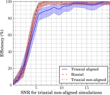
(a)

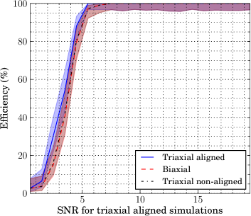
(b)

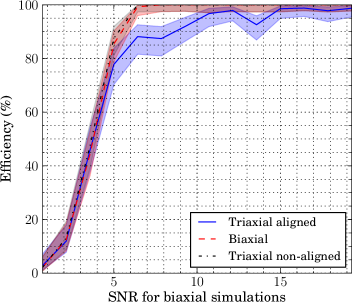
(c)

Figure 8: Each figure shows the efficiencies for signal detection (with a 1% false alarm probability) based on the odds ratios recovered assuming the three different signal models. In (8(a)) the data contained triaxial non-aligned injections, in (8(b)) triaxial aligned injections, and in (8(c)) biaxial injections.

(a)

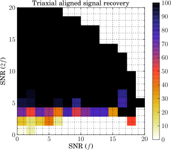
(b)

(c)

Figure 9: The efficiencies for signal detection (with a 1% false alarm probability) based on odds ratios for data containing triaxial non-aligned injections, plotted as a function of the signal SNR in the individual $f$ and $2f$ data streams. The analysis in (9(a)) assumed the (correct) triaxial non-aligned model, while the analyses in (9(b)) and (9(c)) assumed (incorrectly) the triaxial aligned and biaxial models, respectively.

Using the odds ratio values we have calculated, we are also able to compare the Bayesian evidences between signal models rather than just comparing a model to noise. For the biaxial and triaxial non-aligned cases we can take the ratio of odds ratios that we have already calculated as the noise evidence terms will cancel out. However, for the triaxial aligned case we need to include the evidence for there being no signal present in the $f$ data stream as part of the signal model. Therefore the evidence for the triaxial aligned model becomes the product of the evidence for a signal at $2f$ and only noise at $f$. We take model 1 to be favoured over model 2 if $\mathcal{O}_{12}\equiv\mathcal{O}_{1}/\mathcal{O}_{2}>1$. For each model pairing (triaxial aligned versus triaxial non-aligned, triaxial aligned versus biaxial and biaxial versus triaxial non-aligned) we have computed the percentage of our simulated signals for which the numerator model is favoured as a function of SNR, e.g. 50% means that on average either model is equally likely. Results for this can be seen in Fig. 10(a).

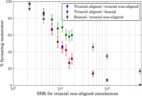
(a)

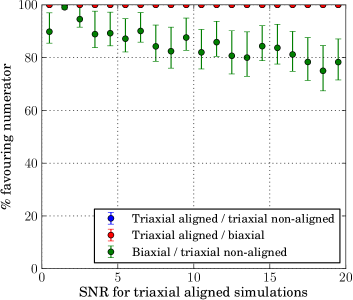
(b)

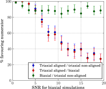
(c)

Figure 10: The percentage of simulations favouring a particular model (see legends) when the simulation contains (10(a)) the full triaxial non-aligned model, (10(b)) the triaxial aligned model, and (10(c)) the biaxial model, as a function of the signal coherent SNR. Note that in (10(b)) the (blue) triaxial aligned/triaxial non-aligned results are barely visible beneath the (red) triaxial aligned/biaxial results.

We see that up to SNRs of $\mathchar 21016\relax 10$ the simpler triaxial aligned model is more often favoured, whilst at greater SNR the triaxial non-aligned and biaxial models become more probable, i.e. the fact that the signal looks more like the triaxial non-aligned and biaxial models starts to overcome the Occam factors disfavouring them. For signals with coherent SNRs of $\mathchar 21016\relax 20$ we see that the simpler triaxial aligned model is still favoured $\mathchar 21016\relax 30\%$ of the time. This is mainly a result of the distribution of our population of simulated signals for which, when the coherent SNR $\mathchar 21016\relax 20$, about a third of the signals have an SNR of $\lesssim 5$ in the $f$ component. Therefore, in these cases the $f$ component is providing very little additional evidence for the triaxial non-aligned, or biaxial models, and the simpler triaxial aligned model is being favoured. A striking point to note is that out to SNRs of somewhere between 20 and 50 the biaxial model is favoured more than 50% of the time over the true triaxial non-aligned model. As noted in Appendix A.2, the biaxial model is just a special case of the triaxial non-aligned model with the constraint that $\Phi^{C}_{22}=2\Phi^{C}_{21}$, so in some small fraction of the simulations this criterion will be fulfilled and the Occam factor will result in the biaxial model being favoured (see discussion below and Fig. 12). However, this does not account for the fraction of the cases that the biaxial model is favoured. To explain that we must look at another degeneracy: when the signal is circularly polarised $\Phi^{C}_{22}$ and $\psi$ become very highly correlated (see, e.g., Fig. 3), and in these cases a combination of $\Phi^{C}_{22}$ and $\psi$ can be found such that $\Phi^{C}_{22}\approx 2\Phi^{C}_{21}$. Therefore these will again look like biaxial signals and the Occam factor will start to favour them. This is demonstrated in Fig. 11, which shows the parameter posterior probability distributions for a triaxial non-aligned signal with SNR $\mathchar 21016\relax 20$ and $|\cos{\iota}|\mathchar 21016\relax 0.5$, even with $|\cos{\iota}|$ some way from unity the correlation between $\Phi^{C}_{22}$ and $\psi$ is still strong. This means that for SNRs $\mathchar 21016\relax 20$ about half the population will still be able to support the biaxial model. Indeed in the case of the signal in Fig. 11 the biaxial model is very slightly favoured over the triaxial non-aligned model by a factor of $\mathchar 21016\relax 1.3$. Even at SNRs as high as 500 this effect still means that $\mathchar 21016\relax 15\mbox{--}20\%$ of triaxial non-aligned signal simulations favour the biaxial model.

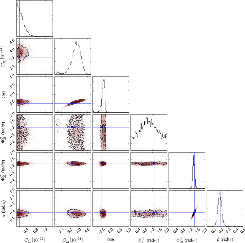
Figure 11: Marginalised posterior probability distribution plots of waveform parameters for an SNR $\mathchar 21016\relax 20$ signal with $\cos{\iota}=-0.49$ covering the minimal parameter ranges of Table 1.

We can also see this effect by looking at three illustrative waveforms, each corresponding to signals with SNR of 500, in the first case picking out a waveform where the biaxial model is favoured by $\mathchar 21016\relax\mathrm{e}^{5.9}$, in the second case the biaxial and triaxial non-aligned models are equally likely, and in the the third case the biaxial model is strongly disfavoured by a factor of $\mathchar 21016\relax\mathrm{e}^{4690}$. The first case is shown in Fig. 12, which happens to be a simulation in which $\Phi^{C}_{22}\approx 2\Phi^{C}_{21}$ and $\cos{\iota}=0.23$, so the waveform is essentially a biaxial waveform and both the biaxial and triaxial non-aligned models recover the correct waveform almost perfectly – the parameters are also recovered consistently for both models. In this case the triaxial non-aligned model provides no extra information, so the Occam factor means that the biaxial model is favoured. The second case is shown in Fig. 13, in which $\Phi^{C}_{22}\not\approx 2\Phi^{C}_{21}$, but $\cos{\iota}=-0.93$. In this case almost identical waveforms are recovered for both models, but due to the $\Phi^{C}_{22}$ and $\psi$ degeneracy the recovered best fit parameters are not the same. The third case is shown in Fig. 14, where again $\Phi^{C}_{22}\not\approx 2\Phi^{C}_{21}$, but $\cos{\iota}=0.23$. This shows that whereas the triaxial non-aligned model produces an excellent fit in both the $f$ and $2f$ data-streams the biaxial model sacrifices any attempt at a good fit in the $2f$ data in favour of getting a very good fit in the higher SNR $f$ data.

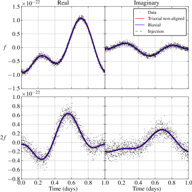
Figure 12: The real and imaginary waveforms for the $f$ and $2f$ data streams of an SNR 500 signal for which the biaxial model is favoured over the triaxial non-aligned model by $\mathchar 21016\relax\mathrm{e}^{5.9}$. The black points represent the simulated data, the overlapping red and blue lines show a distribution of waveforms drawn randomly from the posterior parameter distributions for the triaxial non-aligned and biaxial models respectively, and the dashed black line shows the injected waveform. In this case the lines are nearly impossible to distinguish on the plot, as a consistent waveform is recovered for both models.

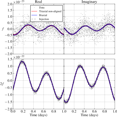
Figure 13: The real and imaginary waveforms for the $f$ and $2f$ data streams of an SNR 500 signal for which the biaxial model and triaxial non-aligned models are equally likely. The black points represent the simulated data, the overlapping red and blue lines show a distribution of waveforms drawn randomly from the posterior parameter distributions for the triaxial non-aligned and biaxial models respectively, and the dashed black line shows the injected waveform. In this case the lines are hard to distinguish between as a consistent waveform is recovered for both models, although in the $f$ data stream there is a minor discrepancy.

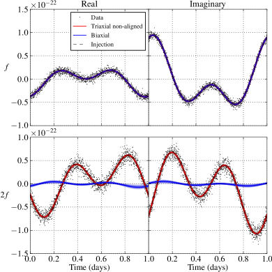
Figure 14: The real and imaginary waveforms for the $f$ and $2f$ data streams of an SNR 500 signal for which the biaxial model is disfavoured over the triaxial non-aligned model by a factor of $\mathchar 21016\relax\mathrm{e}^{4690}$. The black points represent the simulated data, the overlapping red and blue lines show a distribution of waveforms drawn randomly from the posterior parameter distributions for the triaxial non-aligned and biaxial models respectively, and the dashed black line shows the injected waveform. In this case the biaxial model has to sacrifice any close fit in the $2f$ data-stream over producing a very good fit to the higher SNR $f$ data-stream.

5.2.2 Detecting triaxial aligned signals

Using the triaxial aligned injections we have again calculated odds ratios for each model. The efficiencies of detecting these signals for each of the models, using the 1% false alarm probability thresholds given in Section 5.1, are shown in Fig. 8(b).

The triaxial aligned model is just a special case of the two other models and we see that, as it is the simplest model, the best efficiency is achieved when we just use that model. However, the efficiency increase is relatively small compared to more complex models, with those models giving almost 100% efficiency for SNR greater than $\mathchar 21016\relax 7$.

The main advantage of just performing the analysis assuming the triaxial aligned signal model is speed. Using the waveform parameterisation the analysis in this case is $\mathchar 21016\relax 2$ times faster than using the triaxial non-aligned model (the speed ratio does not vary significantly with SNR as the likelihoods in both cases are fairly simple). However, if the signal does contain significant power at $f$ then, as we have seen in Figs 8(a) and 9(b), assuming a purely triaxial aligned signal model could lead to signals being missed.

The signal model comparison is shown in Fig. 10(b). This shows that when a purely triaxial aligned signal is present then that model is always favoured over the more complex models. As we have noted earlier the triaxial aligned model is just a special case of the other models, so this result is purely down to the Occam factor rather than it being a better fit to the data. We also see the Occam factor in play when comparing the biaxial and triaxial non-aligned models, with the biaxial model being favoured for the majority of signals. There is a slow trend towards the triaxial non-aligned model being more favoured. The reasons for this are not entirely clear, but a possible explanation is that the extra free parameter in the triaxial non-aligned model will allow it to more easily accommodate the necessary lack of signal in the $f$ data-stream.

5.2.3 Detecting biaxial signals

Finally, using the biaxial simulations we have calculated odds ratios for each model. Fig. 8(c) shows the efficiencies of detecting these signals for each of the models, using the 1% false alarm probability thresholds given in Section 5.1. The results are similar to those for the triaxial non-aligned injections of Fig. 8(a), with the triaxial aligned model being somewhat less efficient than the biaxial or triaxial non-aligned models, due to its inability to detect signals with low SNR in just the $2f$ component. Again we see that the efficiencies of the triaxial non-aligned and biaxial models are very similar, despite one of them (the latter, in this case) being the correct model.

The signal model comparison is shown in Fig. 10(c). In common with the cases described above, at low SNR the triaxial aligned model is favoured over the other two models. As the SNRs increase, the biaxial and triaxial non-aligned models become more favoured over the triaxial aligned model, by approximately equal amounts, and are more often preferred for SNRs above about $10$. The biaxial model is favoured over the triaxial non-aligned model by a constant amount of $\mathchar 21016\relax 90\%$ over all SNRs except the very smallest ones.

6 Search in real data

We performed a search for gravitational waves from a selection of isolated (i.e. non-binary system) known pulsars using data from the fifth LIGO science run (S5) (Abbott et al., 2009). This is the first gravitational wave search targeted at known pulsars to include an explicit search for a component at the rotation frequency. We consider 43 pulsars that had previously been targeted using an analysis only sensitive to the triaxial aligned model with emission at twice the pulsars’ rotation frequencies (Abbott et al., 2010). We used science mode data from the two LIGO Hanford Observatory detectors (H1 and H2) and the LIGO Livingston Observatory detector (L1) covering 4 November 2005 to 1 October 2007, which was processed into sets of discrete Fourier transforms using 30-min sections of data (called short Fourier transforms, or SFTs; as used in e.g. Aasi et al., 2013). This gave a total of $\mathchar 21016\relax 491$ days of data for H1, $\mathchar 21016\relax 497$ days for H2 and $\mathchar 21016\relax 392$ days for L1. For each pulsar, we filtered the SFTs from each detector using a “spectral interpolation” routine (Davies et al., 2015) to create two narrow-band complex data streams sampled at one per 30 minutes: one with the phase evolution at the pulsars’ rotation frequency removed, and the other with the phase evolution at twice the pulsars’ rotation frequency removed. For each data stream we also produced estimates of the time-varying standard deviation of the corresponding noise.

For each pulsar we performed parameter estimation and calculated the evidence for each of the triaxial aligned, biaxial and triaxial non-aligned models. This allows us to perform model comparison for each source, assess the detection of signals and produce 95% credible region upper limits (bounded at zero) on the waveform model amplitudes $C_{21}$ and $C_{22}$. We show the results, based on a joint analysis of data from all three detectors, in Table 3. As with the analysis in Abbott et al. (2010) we expect amplitude calibration uncertainties of 10% for H1 and H2 and 13% for L1. The table includes results for the triaxial aligned model giving upper limits on the conventionally quoted gravitational wave strain amplitude $h_{0}$ (which in this model is related to $C_{22}$ via $h_{0}=2C_{22}$). These upper limits are broadly consistent (within $\mathchar 21016\relax 25\%$) with those in Abbott et al. (2010), but are not identical due to differences in the processing pipeline (heterodyned, averaged and low-pass filtered (Dupuis & Woan, 2005) vs. Fourier-transformed) and the fact that here we have used a Gaussian likelihood for the data given our model (using a noise estimate for each sample), rather than a Student’s $t$ likelihood with its implied marginalisation over an unknown noise level. From Table 3 we see that the triaxial aligned model is favoured by factors of $\mathchar 21016\relax\mathrm{e}^{12}$ in all cases. Given that the previous gravitational wave search reported in Abbott et al. (2010) found no evidence for triaxial aligned signals (purely based on examination of posterior probability distributions of the estimated signal amplitudes), we can conclude that there is no evidence for biaxial or triaxial non-aligned signals either. However, below we will also assess the significance of the odds ratio for the triaxial non-aligned signal compared to noise, which appears in the results table.

One advantage of using the waveform parameterisation over the source parameterisation is that $C_{21}$ and $C_{22}$ directly represent the search sensitivity at $f$ and $2f$ respectively, whereas $I_{31}$ and $I_{21}$ contribute to both harmonics in a complicated way that cannot be disentangled. However, it is important to note that we currently do not have a good understanding of the physical interpretation of $C_{21}$ and $C_{22}$. It is interesting to note from our results in Table 3 that, although in many cases the detector sensitivities are better at $f$ than $2f$ (see e.g. Fig. 4 of Abbott et al., 2010), we get smaller upper limits on $C_{22}$ for all bar two pulsars (J0024$-$7204C and J2322$+$2057). This because when $\iota=0$ the $f$ signal is zero and $C_{21}$ can extend to arbitrarily large values, which creates a tail on the $C_{21}$ posterior probability distribution leading to the larger upper limits. The tail would be suppressed if a Jeffreys prior were used for the amplitudes, but would still be present at some level as the correlation is a feature of the waveform. Fig. 15 shows an example of the posterior probability distributions for the triaxial non-aligned model for pulsar J0024$-$7204C.

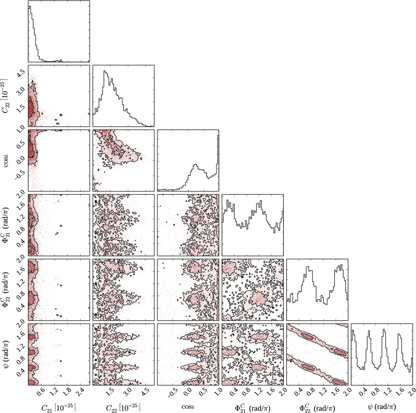
Figure 15: The posterior probability distributions for the waveform parameters of the triaxial non-aligned model found using S5 data for pulsar J0024$-$7204C.

6.1 Results significance

It is useful to have a way to assess whether the signal vs. noise odds ratio value for a particular pulsar is large enough to be considered a detection (or detection candidate). As mentioned earlier, the odds ratio itself tells us how much more probable the signal model is compared to noise given the data, but fluctuations in this value for different noise realisations and the effect of our large amplitude prior ranges mean that an understanding of the potential distribution of values is useful in making a detection decision. We did this in Section 5.1 using simulations of noise-only data to get a distribution of odds ratios when no signal was present, from which we could set a detection threshold, given a chosen false alarm rate. For data in which the noise is purely Gaussian this is straightforward, but with real data we need a way of producing the corresponding noise-only data with the same statistics to get a representative distributions of odds ratios. It is also useful to look at extra information such as the SNR of the maximum a posteriori recovered waveform. Assessing a particular search’s significance using an empirically estimated ‘background’ distribution of some detection statistic versus SNR is common for many searches for transient gravitational waves, where in those cases the ‘background’ is generated through many time-slides of the data.

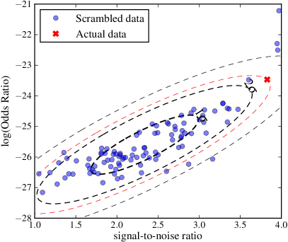
Figure 16: The distribution of log odds ratios (for the triaxial non-aligned model versus noise) against SNR for 100 ‘scrambled’ noise-only realisations of the dataset for pulsar J1024$-$0719. The actual (i.e. not randomised in time) value is plotted as the red cross. Assuming that the noise-only distribution is a bivariate Gaussian, the 1, 2 and $3\sigma$ (or $68.3\%$, $95.4\%$ and $99.7\%$) probability contours are also plotted, along with the probability contour on which the actual value lies.

To estimate a noise-only distribution of log odds ratios for the triaxial non-aligned model versus noise for each pulsar we have made use of the same data as for the real analysis, but have ‘scrambled’ the data by randomly shuffling the time order. This preserves the same noise statistics, but would completely de-cohere any signal present, essentially giving us random realisations of the data. For each pulsar therefore, we shuffled the data 100 times and calculated the log odds ratio for the triaxial non-aligned model versus Gaussian noise, whilst also recording the SNR of the maximum a posteriori recovered signal model. We calculated the correlation matrix of these 100 pairs of log odds ratios and SNR and then, assuming their distribution is a bivariate Gaussian, calculated a set of probability contours in the odds ratio–SNR plane for these. The actual odds ratio and SNR for the pulsar (obtained using the non-scrambled data) can then be placed on the plot, and its location relative to the noise-only distribution’s contour lines gives an indication of its significance. For instance, an actual observation with a percentile contour value $\gtrsim 99.7\%$ would be outside $3\sigma$ of the noise-only distribution (under the assumption of a bivariate Gaussian distribution). Of our results the actual value lying on the highest percentile is for J1024$-$0719 at 98.05% (or equivalently at $2.34\sigma$ from the mean of the scrambled data distribution). This is shown in Fig. 16. Unsurprisingly, given the use of 100 scrambled data realisations there are three points further out in the distribution, and we can conclude that this is not a significant event (although we note that in this case the distribution of scrambled data points is not quite a bivariate Gaussian as the three outlier points are beyond the $3\sigma$ contour).

The use of the SNR in these plots provides some further level of discrimination from interference compared to real signals in that data could return a high SNR signal (e.g. from a spectral line) that has a low odds ratio due to not matching the signal model or being incoherent between detectors. Such a situation would give an obvious outlier on plots such as Fig. 16. Real signals would be expected to have large values of both odds ratio and SNR and thus lie roughly along the diagonal of such plots.

Table 3: Upper limits on gravitational wave amplitudes, and log odds ratios comparing the triaxial aligned model (1), biaxial model (2) and triaxial non-aligned model (3) signal models, for 43 isolated pulsars using LIGO S5 data. Also given is the percentile probability contour in the odds ratio (of triaxial non-aligned signal verses noise)—SNR plane of the background distribution on which the actual data point sits.

PSR	$f$ (Hz)	$2f$ (Hz)	$C_{21}^{95\%}$	$C_{22}^{95\%}$	$h_{0}^{95\%}$	$\ln{\mathcal{O}_{12}}$	$\ln{\mathcal{O}_{13}}$	$\ln{\mathcal{O}_{23}}$	percentile
J0024$-$7204C	$173.7$	$347.4$	$6.5\!\times\!10^{-26}$	$3.4\!\times\!10^{-25}$	$6.5\!\times\!10^{-25}$	$12.8$	$12.8$	$-0.8$	94.5
J0024$-$7204D	$186.7$	$373.3$	$5.8\!\times\!10^{-26}$	$2.0\!\times\!10^{-26}$	$4.7\!\times\!10^{-26}$	$13.4$	$13.4$	$\hbox{$\phantom{-}$}0.7$	81.3
J0024$-$7204F	$381.2$	$762.3$	$1.1\!\times\!10^{-25}$	$4.7\!\times\!10^{-26}$	$8.2\!\times\!10^{-26}$	$11.1$	$11.1$	$\hbox{$\phantom{-}$}0.7$	46.0
J0024$-$7204G	$247.5$	$495.0$	$1.5\!\times\!10^{-25}$	$4.2\!\times\!10^{-26}$	$8.5\!\times\!10^{-26}$	$12.1$	$12.1$	$-1.4$	59.8
J0024$-$7204L	$230.1$	$460.2$	$6.4\!\times\!10^{-26}$	$2.8\!\times\!10^{-26}$	$5.9\!\times\!10^{-26}$	$12.5$	$12.5$	$\hbox{$\phantom{-}$}0.3$	44.7
J0024$-$7204M	$272.0$	$544.0$	$7.2\!\times\!10^{-26}$	$3.6\!\times\!10^{-26}$	$7.4\!\times\!10^{-26}$	$12.6$	$12.6$	$-0.5$	43.2
J0024$-$7204N	$327.4$	$654.9$	$1.5\!\times\!10^{-25}$	$3.2\!\times\!10^{-26}$	$7.3\!\times\!10^{-26}$	$12.3$	$12.3$	$-0.1$	58.1
J0711$-$6830	$182.1$	$364.2$	$9.5\!\times\!10^{-26}$	$2.0\!\times\!10^{-26}$	$4.2\!\times\!10^{-26}$	$12.1$	$12.1$	$-0.2$	23.2
J1024$-$0719	$193.7$	$387.4$	$1.2\!\times\!10^{-24}$	$3.3\!\times\!10^{-26}$	$6.3\!\times\!10^{-26}$	$11.0$	$11.0$	$-0.3$	98.0
J1730$-$2304	$123.1$	$246.2$	$7.8\!\times\!10^{-26}$	$3.2\!\times\!10^{-26}$	$6.6\!\times\!10^{-26}$	$13.1$	$13.1$	$\hbox{$\phantom{-}$}1.3$	95.1
J1744$-$1134	$245.4$	$490.9$	$6.7\!\times\!10^{-26}$	$4.3\!\times\!10^{-26}$	$8.3\!\times\!10^{-26}$	$13.2$	$13.2$	$\hbox{$\phantom{-}$}0.8$	63.8
J1748$-$2446C	$118.5$	$237.1$	$6.2\!\times\!10^{-26}$	$2.1\!\times\!10^{-26}$	$4.4\!\times\!10^{-26}$	$12.4$	$12.4$	$\hbox{$\phantom{-}$}0.7$	43.8
J1748$-$2446D	$212.1$	$424.3$	$3.8\!\times\!10^{-25}$	$3.4\!\times\!10^{-26}$	$7.5\!\times\!10^{-26}$	$12.7$	$12.7$	$-0.3$	36.7
J1748$-$2446F	$180.5$	$361.0$	$7.7\!\times\!10^{-26}$	$3.1\!\times\!10^{-26}$	$6.4\!\times\!10^{-26}$	$12.2$	$12.2$	$\hbox{$\phantom{-}$}0.0$	60.0
J1748$-$2446H	$203.0$	$406.0$	$7.0\!\times\!10^{-26}$	$3.5\!\times\!10^{-26}$	$6.9\!\times\!10^{-26}$	$12.9$	$12.9$	$-0.2$	61.1
J1748$-$2446K	$336.7$	$673.5$	$2.1\!\times\!10^{-25}$	$3.2\!\times\!10^{-26}$	$7.0\!\times\!10^{-26}$	$11.3$	$11.3$	$\hbox{$\phantom{-}$}0.1$	61.6
J1748$-$2446L	$445.5$	$891.0$	$6.3\!\times\!10^{-25}$	$6.9\!\times\!10^{-26}$	$1.7\!\times\!10^{-25}$	$11.4$	$11.4$	$-0.3$	81.0
J1748$-$2446R	$198.9$	$397.7$	$1.1\!\times\!10^{-25}$	$3.8\!\times\!10^{-26}$	$8.7\!\times\!10^{-26}$	$12.7$	$12.7$	$\hbox{$\phantom{-}$}2.2$	60.0
J1748$-$2446S	$163.5$	$327.0$	$5.5\!\times\!10^{-26}$	$2.6\!\times\!10^{-26}$	$5.2\!\times\!10^{-26}$	$12.6$	$12.6$	$-0.7$	31.5
J1748$-$2446T	$141.1$	$282.3$	$8.3\!\times\!10^{-26}$	$2.7\!\times\!10^{-26}$	$5.4\!\times\!10^{-26}$	$13.7$	$13.7$	$\hbox{$\phantom{-}$}0.2$	54.9
J1748$-$2446aa	$172.8$	$345.5$	$1.1\!\times\!10^{-25}$	$9.9\!\times\!10^{-26}$	$2.1\!\times\!10^{-25}$	$12.7$	$12.7$	$\hbox{$\phantom{-}$}0.1$	63.0
J1748$-$2446ab	$195.3$	$390.6$	$6.0\!\times\!10^{-26}$	$2.6\!\times\!10^{-26}$	$5.1\!\times\!10^{-26}$	$13.1$	$13.1$	$\hbox{$\phantom{-}$}0.8$	63.1
J1748$-$2446ac	$196.6$	$393.2$	$7.9\!\times\!10^{-26}$	$2.3\!\times\!10^{-26}$	$4.2\!\times\!10^{-26}$	$12.8$	$12.8$	$-0.1$	52.9
J1748$-$2446af	$302.6$	$605.3$	$5.5\!\times\!10^{-25}$	$5.4\!\times\!10^{-26}$	$1.1\!\times\!10^{-25}$	$12.0$	$12.0$	$-3.1$	95.1
J1748$-$2446ag	$224.8$	$449.6$	$7.5\!\times\!10^{-26}$	$5.3\!\times\!10^{-26}$	$1.1\!\times\!10^{-25}$	$12.3$	$12.3$	$\hbox{$\phantom{-}$}0.3$	90.9
J1748$-$2446ah	$201.4$	$402.8$	$7.1\!\times\!10^{-26}$	$3.1\!\times\!10^{-26}$	$6.2\!\times\!10^{-26}$	$12.8$	$12.8$	$-1.0$	74.2
J1801$-$1417	$275.9$	$551.7$	$1.2\!\times\!10^{-25}$	$2.9\!\times\!10^{-26}$	$5.8\!\times\!10^{-26}$	$11.7$	$11.7$	$-0.0$	29.4
J1803$-$30	$140.8$	$281.6$	$6.9\!\times\!10^{-26}$	$3.3\!\times\!10^{-26}$	$6.5\!\times\!10^{-26}$	$11.7$	$11.7$	$\hbox{$\phantom{-}$}0.9$	84.5
J1823$-$3021A	$183.8$	$367.6$	$8.7\!\times\!10^{-26}$	$2.2\!\times\!10^{-26}$	$4.1\!\times\!10^{-26}$	$14.1$	$14.1$	$\hbox{$\phantom{-}$}0.6$	82.0
J1824$-$2452A	$327.4$	$654.8$	$8.4\!\times\!10^{-26}$	$3.9\!\times\!10^{-26}$	$8.4\!\times\!10^{-26}$	$13.2$	$13.2$	$\hbox{$\phantom{-}$}0.8$	91.2
J1824$-$2452B	$152.7$	$305.5$	$7.7\!\times\!10^{-26}$	$2.5\!\times\!10^{-26}$	$5.2\!\times\!10^{-26}$	$13.6$	$13.6$	$-0.1$	94.3
J1824$-$2452E	$184.5$	$369.1$	$5.9\!\times\!10^{-26}$	$3.5\!\times\!10^{-26}$	$6.7\!\times\!10^{-26}$	$12.2$	$12.2$	$-0.3$	47.4
J1824$-$2452F	$408.0$	$815.9$	$1.4\!\times\!10^{-24}$	$4.6\!\times\!10^{-26}$	$9.1\!\times\!10^{-26}$	$11.9$	$11.9$	$\hbox{$\phantom{-}$}0.6$	34.5
J1843$-$1113	$541.8$	$1083.6$	$1.8\!\times\!10^{-25}$	$7.6\!\times\!10^{-26}$	$1.5\!\times\!10^{-25}$	$12.5$	$12.5$	$-0.2$	97.0
J1905+0400	$264.2$	$528.5$	$6.2\!\times\!10^{-26}$	$3.8\!\times\!10^{-26}$	$7.8\!\times\!10^{-26}$	$12.4$	$12.4$	$\hbox{$\phantom{-}$}0.6$	47.8
J1910$-$5959B	$119.6$	$239.3$	$5.9\!\times\!10^{-26}$	$1.9\!\times\!10^{-26}$	$4.2\!\times\!10^{-26}$	$12.8$	$12.8$	$-0.8$	49.3
J1910$-$5959C	$189.5$	$379.0$	$6.0\!\times\!10^{-26}$	$2.2\!\times\!10^{-26}$	$4.6\!\times\!10^{-26}$	$12.1$	$12.1$	$-1.9$	70.9
J1910$-$5959D	$110.7$	$221.4$	$7.7\!\times\!10^{-26}$	$1.4\!\times\!10^{-26}$	$2.9\!\times\!10^{-26}$	$12.6$	$12.6$	$\hbox{$\phantom{-}$}1.3$	50.6
J1910$-$5959E	$218.7$	$437.5$	$6.3\!\times\!10^{-26}$	$2.1\!\times\!10^{-26}$	$4.6\!\times\!10^{-26}$	$12.4$	$12.4$	$\hbox{$\phantom{-}$}0.4$	32.7
J1911+1347	$216.2$	$432.3$	$2.3\!\times\!10^{-24}$	$2.5\!\times\!10^{-26}$	$6.0\!\times\!10^{-26}$	$12.2$	$12.2$	$-0.1$	51.7
J1939+2134	$641.9$	$1283.9$	$2.4\!\times\!10^{-25}$	$7.5\!\times\!10^{-26}$	$1.6\!\times\!10^{-25}$	$11.4$	$11.4$	$-0.1$	37.2
J2124$-$3358	$202.8$	$405.6$	$8.3\!\times\!10^{-26}$	$2.1\!\times\!10^{-26}$	$4.7\!\times\!10^{-26}$	$12.5$	$12.5$	$-0.4$	57.0
J2322+2057	$208.0$	$415.9$	$4.3\!\times\!10^{-26}$	$4.4\!\times\!10^{-26}$	$8.8\!\times\!10^{-26}$	$13.9$	$13.9$	$-0.2$	52.5

7 Conclusions

We have investigated detection and parameter estimation issues for the model of gravitational wave emission from rotating neutron stars proposed in Jones (2010). The model is based on the star having a triaxial crust, coupled to an interior superfluid. In the generic case of a triaxial non-aligned star, there is emission at both the spin frequency $f$ and at $2f$. We have also considered two special cases, of a biaxial star (also with emission at $f$ and $2f$), and a triaxial aligned one (emission only at $2f$), the last of these being the case conventionally assumed in gravitational wave searches.

We have found that in the generic case of emission from a triaxial non-aligned star, the set of physical parameters originally used in Jones (2010), the ‘source parameters’, are correlated in a highly complex way. However, a re-parameterisation in terms of complex waveform amplitudes using the ‘waveform parameters’ described in Jones (2015) breaks this degeneracy. When using a stochastic sampling method (such as nested sampling) to estimate parameter probability distributions from data containing such a signal, the complexity of the source parameter space makes a search there roughly half as computationally efficient as one in the waveform parameter space.

For a signal described by the triaxial non-aligned model, we showed that estimates of many of the true individual source parameters, including the important parameters giving the asymmetry of the moment of inertia tensor, will always be poorly constrained due to the degeneracies in the model. This may limit the astrophysical information that can be extracted on such a source. We also note the (often overlooked) fact when discussing parameter estimation for these sources that for any signal there is a degeneracy in the full physically allowed parameter space that means the signal can only ever be constrained to a number of equally likely modes.

Working in the waveform parameterisation, and assuming stationary Gaussian noise in the data, we have used simulations to calculate the odds ratio for three different signal models compared to noise alone. We find that for a 1% false alarm rate, calculated from an odds ratio threshold value, all three models have efficiencies of close to 100% for purely triaxial aligned signals with SNR $\gtrsim 6$. The simplicity of the triaxial aligned model compared to the others does make it slightly more efficient in this case, but only marginally so. For signals from the triaxial non-aligned and biaxial models, with significant power at $f$, when assuming either of those models, efficiencies are close to 100% for SNRs $\gtrsim 6$, while assuming the triaxial aligned model leads to some loss in efficiency, due to some proportion of signals having very little power at $2f$. Without some idea of the true distribution of signals strengths between $f$ and $2f$ we cannot say whether only searching a $2f$ would cause any real signals to be missed. But, the ease of searching at both frequencies, and the only very minor efficiency loss, makes performing such a search seem sensible in the future.

When comparing model evidences we find that for simulations containing any of the three models, at very low SNR ($\lesssim 2.5$) the triaxial aligned model is always favoured. If the simulated signal is from the triaxial aligned model then this is always favoured over the other two models, whilst there is a strong preference for the biaxial as compared to the triaxial non-aligned one due to the biaxial model being the simpler one. For simulations containing triaxial non-aligned signals, the triaxial non-aligned and biaxial models are favoured over the triaxial aligned model for coherent SNRs $\gtrsim 10$. We see a similar situation in simulations containing biaxial injections: at low SNR the triaxial aligned model is favoured, but at higher SNR the biaxial and triaxial non-aligned models become favoured over the triaxial aligned one, while the biaxial model becomes favoured over the triaxial non-aligned one.

Our results show that, even though to detect all triaxial non-aligned (or biaxial) signals at SNR 20 one should use the triaxial non-aligned (or biaxial) model when computing the evidence, the Occam factor still significantly penalises a reasonable percentage of those models when deciding which best fits the data. As such it is worth noting that even at high SNR it is often not possible to distinguish a triaxial non-aligned signal from a biaxial one. However, the cost of searching for a triaxial non-aligned signal compared to a biaxial signal is relatively minor, so there is no reason to not include such a search in the future.

Having developed the machinery needed to search for such signals, we then applied our methods to real gravitational wave detector data. Specifically, data from the S5 LIGO science run was used to search for two-harmonic signals from 43 known pulsars with accurately known timing solutions, whose spin frequencies lie within the LIGO band. We found no gravitational wave signals, and so upper limits were given on the amplitude-like parameters $C_{21}$ and $C_{22}$ on the triaxial non-aligned model. This is the first time gravitational wave detector data has been searched for such signals. The techniques developed here will be applied to the more sensitive data soon to come from the new generation of advanced gravitational wave detectors (Aasi et al., 2015; Acernese et al., 2015).

There is further work to do on the choice of prior probability distributions that one assumes for the parameters, particularly for the amplitude-like parameters. A simple choice, uniform up to some fixed maximum amplitude, was used here, but other choices are possible and will affect the results obtained. Closely related to this is the issue of the physical interpretation of the parameters $C_{21}$ and $C_{22}$; it is useful to consider whether they have a direct physical interpretation. Their maximum values are presumably related to the shear modulus and breaking strain of the crust, and also to the strength of the interaction between the superfluid and non-superfluid parts of the star, but the relation is not obvious, and is clearly worthy of further study.

Appendix A Relating the source and waveform parameters

In this appendix we briefly describe the relation between the source parameters and the waveform parameters, for all three of our chosen physical models. Full details can be found in Jones (2015). Note that there a few small differences in notation between the equations given here and those of Jones (2015). The angle $\psi$ of Jones (2015) is denoted by $\lambda$ in this paper, as we reserve the symbol $\psi$ for the polarisation angle, describing the projection of the star’s spin axis on the plane of the sky. Also, the quantities denoted by $(\tilde{C}_{22},\tilde{C}_{21})$ of Jones (2015) are denoted by $(C_{22},C_{21})$ in this paper.

A.1 Triaxial non-aligned case

For the triaxial non-aligned case, the waveform is given in terms of source parameters by Eqns (2.1) and (2.1), and by Eqns (6) and (7) in terms of waveform parameters. It can be shown that the relationship between the five source parameters $(I_{21},I_{31},\theta,\phi_{0},\lambda)$ and the four source parameters $(C_{21},\Phi^{\rm C}_{21},C_{22},\Phi^{\rm C}_{22})$ is as follows:

$$C_{22}= 2\{[I_{21}(\sin^{2}\lambda-\cos^{2}\lambda\cos^{2}\theta)-I_{31}\sin^{2}\theta]^{2}+$$

$$(I_{21}\sin 2\lambda\cos\theta)^{2}\}^{1/2},$$ (22)

$$C_{21}= 2\{(I_{21}\sin 2\lambda\sin\theta)^{2}+(I_{21}\cos^{2}\lambda-I_{31})^{2}\sin^{2}2\theta\}^{1/2},$$ (23)

$$\tan[2\phi_{0}-\Phi^{C}_{22}]= \frac{I_{21}\sin 2\lambda\cos\theta}{I_{21}(\sin^{2}\lambda-\cos^{2}\lambda\cos^{2}\theta)-I_{31}\sin^{2}\theta},$$ (24)

$$\tan[\phi_{0}-\Phi^{C}_{21}]= \frac{(I_{21}\cos^{2}\lambda-I_{31})\sin 2\theta}{I_{21}\sin 2\lambda\sin\theta};$$ (25)

see equations (62)–(65) of Jones (2015). Given the set of five source parameters one can calculate unique values for the four waveform parameters. However, for a set of four waveform parameters, the corresponding solution for the five source parameters will have one degree of freedom, generating the sorts of complex structure in source parameter space seen in Figs 2 and 4.

A.2 Biaxial case

If we set $I_{21}=0$ in Eqns (2.1) and (2.1) we obtain the biaxial signal in terms of source parameters:

$$h_{+}^{2f}= -2I_{31}(1+\cos^{2}\iota)\sin^{2}\theta\cos 2(\Omega t+\phi_{0}),$$ (26)

$$h_{\times}^{2f}= -4I_{31}\cos\iota\sin^{2}\theta\sin 2(\Omega t+\phi_{0}),$$ (27)

$$h_{+}^{f}= -I_{31}\sin\iota\cos\iota\sin 2\theta\sin(\Omega t+\phi_{0}),$$ (28)

$$h_{\times}^{f}= I_{31}\sin\iota\sin 2\theta\cos(\Omega t+\phi_{0}),$$ (29)

where we have separated out the ‘$+$’ and ‘$\times$’ polarisation components.

It can be shown that the corresponding waveform parameterisation can be written as Eqn. (6) and (7), with the extra condition

$$\Phi^{C}_{22}=2\Phi^{C}_{21};$$ (30)

see equation (90) of Jones (2015). The relation between the source and waveform parameters can be shown to be

$$\theta= \tan^{-1}\left(\frac{2C_{22}}{C_{21}}\right),$$ (31)

$$I_{31}= -\frac{1}{2}C_{22}\left[1+\left(\frac{C_{21}}{2C_{22}}\right)^{2}\right],$$ (32)

$$\phi_{0}= \Phi^{C}_{21}-\frac{\pi}{2};$$ (33)

see equations (82), (88) and (89) of Jones (2015).

A.3 Triaxial aligned case

If we set $\theta=0$ in Eqns (2.1) and (2.1) we obtain the triaxial aligned signal in terms of source parameters. There in no signal at frequency $f$, leaving only:

$$h^{2f}_{+}= -2I_{21}(1+\cos^{2}\iota)\cos 2[\Omega t+(\phi_{0}+\lambda)],$$ (34)

$$h^{2f}_{\times}= -4I_{21}\cos\iota\sin 2[\Omega t+(\phi_{0}+\lambda)].$$ (35)

The angles $\phi_{0}$ and $\lambda$ are now degenerate, with only their sum appearing in the waveform. This sum can now be taken as replacing the separate parameters, or else one can simply set one of them to a constant value and search over the other (e.g. set $\lambda=0$ and search over $\phi_{0}$).

The corresponding waveform parameterisation has $C_{21}=0$ so that we only have the $2f$ signal given by Eqn. (7), with the source and waveform parameters being related by

$$I_{21}= \frac{1}{2}C_{22},$$ (36)

$$2(\phi_{0}+\lambda)= \Phi^{C}_{22};$$ (37)

see equations (103) and (104) of Jones (2015).

Appendix B Algorithm to fill in the full source parameter space

In this appendix we present (as pseudo-code) the algorithm used to map the minimal source parameters space, whose ranges were given in Table 2, to the full parameter space.

Algorithm 1 Transformations required to map from the minimal range in the source model parameter space to the full space. The values with the superscript ‘min’ represent the original samples from the minimal parameter range.

1:for $i\leftarrow 1\textbf{ to }4$ do

2:     draw a random unique set consisting of one quarter of the samples, such that $\mn@boldsymbol{j}_{i}$ is a vector of those samples’ indices for loop $i$

3:     $\psi(\mn@boldsymbol{j}_{i})=\psi^{\rm min}(\mn@boldsymbol{j}_{i})+(i-1)\pi/2$

4:     $\theta(\mn@boldsymbol{j}_{i})=\theta^{\rm min}(\mn@boldsymbol{j}_{i})$

5:     $\phi_{0}(\mn@boldsymbol{j}_{i})=\phi^{\rm min}_{0}(\mn@boldsymbol{j}_{i})$

6:     $\lambda(\mn@boldsymbol{j}_{i})=\lambda^{\rm min}(\mn@boldsymbol{j}_{i})$

7:     $I_{21}(\mn@boldsymbol{j}_{i})=I^{\rm min}_{21}(\mn@boldsymbol{j}_{i})$

8:     $I_{31}(\mn@boldsymbol{j}_{i})=I^{\rm min}_{31}(\mn@boldsymbol{j}_{i})$

9:     for $k\leftarrow 1\textbf{ to }i$ do

10:         $\theta_{\rm new}=\arctan{\left(\frac{\sqrt{1-(\sin{\theta(\mn@boldsymbol{j}_{i})}\sin{\lambda(\mn@boldsymbol{j}_{i})})^{2}}}{\sin{\theta(\mn@boldsymbol{j}_{i})}\sin{\lambda(\mn@boldsymbol{j}_{i})}}\right)}$

11:          $\phi_{0}(\mn@boldsymbol{j}_{i})=$ $\arctan{\left(\frac{\cos{\phi_{0}(\mn@boldsymbol{j}_{i})}\cos{\lambda(\mn@boldsymbol{j}_{i})}-\sin{\phi_{0}(\mn@boldsymbol{j}_{i})}\cos{\theta(\mn@boldsymbol{j}_{i})}\sin{\lambda(\mn@boldsymbol{j}_{i})}}{-\cos{\phi_{0}(\mn@boldsymbol{j}_{i})}\cos{\theta(\mn@boldsymbol{j}_{i})}\sin{\lambda(\mn@boldsymbol{j}_{i})}-\sin{\phi_{0}(\mn@boldsymbol{j}_{i})}\cos{\lambda(\mn@boldsymbol{j}_{i})}}\right)}$

12:         $\lambda(\mn@boldsymbol{j}_{i})=\arctan{\left(\frac{-\cos{\theta(\mn@boldsymbol{j}_{i})}}{\sin{\theta(\mn@boldsymbol{j}_{i})}\cos{\lambda(\mn@boldsymbol{j}_{i})}}\right)}$

13:         $I_{21}(\mn@boldsymbol{j}_{i})=I_{31}(\mn@boldsymbol{j}_{i})-I_{21}(\mn@boldsymbol{j}_{i})$

14:         $I_{31}(\mn@boldsymbol{j}_{i})=I_{31}(\mn@boldsymbol{j}_{i})$

15:         $\theta_{i}=\theta_{\rm new}$

16:     end for

17:end for

18:randomly select half the samples, such that $\mn@boldsymbol{k}_{1}$ is a vector of those sample indices

19:apply $\lambda(\mn@boldsymbol{k}_{1})=\lambda(\mn@boldsymbol{k}_{1})+\pi$

20:randomly select half the samples, such that $\mn@boldsymbol{k}_{2}$ is a vector of those sample indices

21:apply $\theta(\mn@boldsymbol{k}_{2})=\pi-\theta(\mn@boldsymbol{k}_{2})$, $\phi_{0}(\mn@boldsymbol{k}_{2})=\phi_{0}(\mn@boldsymbol{k}_{2})+\pi$ and $\lambda(\mn@boldsymbol{k}_{2})=-\lambda(\mn@boldsymbol{k}_{2})$

22:$\phi_{0}=\phi_{0}\ (\textrm{mod}\ 2\pi)$

23:$\lambda=\lambda\ (\textrm{mod}\ 2\pi)$

References

- Aasi et al. (2013) Aasi J., et al., 2013, \prd, 87, 042001, arXiv:1207.7176
- Aasi et al. (2014) Aasi J., et al., 2014, \apj, 785, 119, arXiv:1309.4027
- Aasi et al. (2015) Aasi J., et al., 2015, Classical and Quantum Gravity, 32, 074001, arXiv:1411.4547, doi:10.1088/0264-9381/32/7/074001
- Abadie et al. (2011) Abadie J., et al., 2011, \apj, 737, 93, arXiv:1104.2712
- Abbott et al. (2005) Abbott B., et al., 2005, \prl, 94, 181103, arXiv:gr-qc/0410007
- Abbott et al. (2007) Abbott B., et al., 2007, \prd, 76, 042001, arXiv:gr-qc/0702039
- Abbott et al. (2008) Abbott B., et al., 2008, \apjl, 683, L45, arXiv:0805.4758
- Abbott et al. (2009) Abbott B. P., et al., 2009, Rept. Prog. Phys., 72, 076901, arXiv:0711.3041
- Abbott et al. (2010) Abbott B. P., et al., 2010, \apj, 713, 671, arXiv:0909.3583
- Acernese et al. (2015) Acernese F., et al., 2015, Classical and Quantum Gravity, 32, 024001, arXiv:1408.3978, doi:10.1088/0264-9381/32/2/024001
- Bejger & Królak (2014) Bejger M., Królak A., 2014, Classical and Quantum Gravity, 31, 105011, arXiv:1312.5478
- Cameron (2011) Cameron E., 2011, PASA, 28, 128, arXiv:1012.0566
- Davies et al. (2015) Davies G., Pitkin M., Woan G., 2015, in preparation
- Dupuis & Woan (2005) Dupuis R. J., Woan G., 2005, \prd, 72, 102002, arXiv:gr-qc/0508096
- Foreman-Mackey et al. (2014) Foreman-Mackey D., et al., 2014, triangle.py v0.1.1, doi:10.5281/zenodo.11020
- Gill (2012) Gill C., 2012, PhD thesis, University of Glasgow
- Jeffreys (1998) Jeffreys H., 1998, Theory of Probability, 3 edn. Oxford University Press
- Jones (2010) Jones D. I., 2010, \mnras, 402, 2503, arXiv:0909.4035
- Jones (2015) Jones D. I., 2015, arXiv:1501.05832, arXiv:1501.05832
- Jones & Andersson (2001) Jones D. I., Andersson N., 2001, \mnras, 324, 811, arXiv:astro-ph/0011063
- Jones & Andersson (2002) Jones D. I., Andersson N., 2002, \mnras, 331, 203, arXiv:gr-qc/0106094
- Manchester et al. (2005) Manchester R. N., Hobbs G. B., Teoh A., Hobbs M., 2005, \aj, 129, 1993, arXiv:astro-ph/0412641
- Pitkin (2011) Pitkin M., 2011, \mnras, 415, 1849, arXiv:1103.5867
- Skilling (2006) Skilling J., 2006, Bayesian Analysis, 1, 833
- Veitch et al. (2015) Veitch J., et al., 2015, \prd, 91, 042003, arXiv:1409.7215
- Veitch & Vecchio (2010) Veitch J., Vecchio A., 2010, \prd, 81, 062003, arXiv:0911.3820
- Zimmermann & Szedenits (1979) Zimmermann M., Szedenits Jr. E., 1979, \prd, 20, 351