$a_{0}(980)$ revisited

Abstract

Light scalar hadrons can be understood as dynamically generated resonances. These arise as ‘companion poles’ in the propagators of quark-antiquark seed states when accounting for meson-loop contributions to the self-energies of the latter. Along this line, we extend previous calculations of Törnqvist and Roos and of Boglione and Pennington, where the resonance $a_{0}(980)$ appears as companion pole in the propagator of $a_{0}(1450)$ which is predominantly a quark-antiquark state. We also construct an effective Lagrangian where $a_{0}(1450)$ couples to pseudoscalar mesons with both non-derivative and derivative interactions. Computing the one-loop self-energy, we demonstrate that the propagator has two poles: a companion pole corresponding to $a_{0}(980)$ and a pole of the seed state $a_{0}(1450)$. The positions of these poles are in quantitative agreement with experimental data.

I Introduction

The majority of mesons can be understood as being predominantly quark-antiquark states Olive et al. (2014). Yet, various unconventional mesonic states such as glueballs, hybrids, and four-quark states are expected Amsler and Törnqvist (2004); *amslerrev2. One particular type of four-quark meson is that of a ‘dynamically generated’ state Close and Törnqvist (2002); Peláez (2015); *pelaez; *pelaez2; Oller and Oset (1997); *oller2; *oller3; Oller and Oset (1999); Jamin et al. (2000); *oller6; van Beveren et al. (2006); Morgan and Pennington (1993); van Beveren et al. (1986); Törnqvist (1995); *tornqvist2; Boglione and Pennington (1997, 2002); Zhou and Xiao (2011). Although there are recent works on the compositeness of (dynamically generated) resonances – see e.g. Refs. Guo and Oller (2015); Albaladejo and Oller (2012), where the former also provides a method to quantify the weight of the two-body components of a resonance – a generally accepted definition of dynamical generation does not exist Giacosa (2009). An interesting version of this idea was put forward in Refs. van Beveren et al. (1986); Törnqvist (1995); *tornqvist2; Boglione and Pennington (1997, 2002). Consider, for instance, a single seed state, e.g. a quark-antiquark meson with certain quantum numbers. This state interacts with other mesons, giving rise to loop contributions in the corresponding self-energy. These shift the pole of the seed state and, moreover, a(t least one) new pole may appear. The latter, also denoted as a companion pole, corresponds to a dynamically generated resonance. As a consequence, two resonances have emerged from a single seed state. In this work, we aim to review some previous works and deepen the understanding of the resonance $a_{0}(980)$ as a dynamically generated state.

There is a growing consensus that the scalar resonances $f_{0}(1370)$, $f_{0}(1500)$, $K_{0}^{\ast}(1430)$, and $a_{0}(1450)$ are predominantly quark-antiquark states; see for example Refs. Amsler and Close (1995); *close2; *close3; *close4; *close5; *close6; Giacosa (2007); Gallas et al. (2010); *eLSM1-2; *eLSM1-3; Parganlija et al. (2013); Oller and Oset (1999); Jamin et al. (2000); *oller6; Zhou and Xiao (2011) [recent studies Janowski et al. (2014); Gui et al. (2013) agree in interpreting the resonance $f_{0}(1710)$ as predominantly gluonic]. Then, the light scalar states $f_{0}(500)$, $f_{0}(980)$, $K_{0}^{\ast}(800)$, and $a_{0}(980)$ are (most likely) predominantly four quark-states [see e.g. Refs. Jaffe (1977a); *jaffe2; Maiani et al. (2004); ’t Hooft et al. (2008); Fariborz (2004); *fariborz2; Napsuciale and Rodriguez (2004); Krehl and Speth (1997); *molecular2; *molecular3; *molecular4; *molecular5; Oller and Oset (1997); *oller2; *oller3; Oller and Oset (1999); Jamin et al. (2000); *oller6; Giacosa (2007); Zhou and Xiao (2011) and refs. therein]. As we shall show in the following for the heavy scalar–isovector seed state $a_{0}(1450)$, the coupling of this state to $\pi\eta,K\bar{K}$, and $\pi\eta^{\prime}$ dynamically generates the light $a_{0}(980)$ as a particular type of four-quark meson.

Törnqvist and Roos Törnqvist (1995); *tornqvist2 (in the following denoted as TR) and later Boglione and Pennington Boglione and Pennington (1997, 2002) (denoted as BP) studied the mechanism of dynamical generation through meson-loop contributions to the self-energy. Here, we extend their studies (Sec. II) and compare numerical results for the poles of the propagator to the latest experimental data Olive et al. (2014). It turns out that (depending on the assignment of the poles to physical resonances) the widths of both the seed state $a_{0}(1450)$ and the dynamically generated state $a_{0}(980)$ are by a factor of $2$ larger than the experimental values. Moreover, the mass of $a_{0}(1450)$ is too large (by $100$ MeV in TR and by $400$ MeV in BP). It thus seems that, while qualitatively feasible, the dynamical generation of resonances as companion poles in the propagator does not yield results that are in quantitative agreement with experimental data.

In this work, we show that this is actually not true and that the mechanism of dynamical generation produces results which are in quantitative agreement with the data. To this end, we introduce a Lagrangian inspired by the recently developed extended Linear Sigma Model (eLSM) Gallas et al. (2010); *eLSM1-2; *eLSM1-3; Parganlija et al. (2013). Here, the mesons interact via derivative and non-derivative couplings (Sec. III). In our case, the Lagrangian contains a single scalar–isovector $a_{0}$ seed state which corresponds to the resonance $a_{0}(1450)$. A careful analysis of the pole structure of the corresponding propagator shows that it is indeed possible to obtain a narrow resonance with mass around $1$ GeV, the pole coordinates of which fit quite well with those of the physical $a_{0}(980)$ resonance, and simultaneously obtain a pole for the seed state in agreement with that for the $a_{0}(1450)$ Olive et al. (2014). Finally, we also investigate the use of Feynman rules in the context of quantum field theories with derivative interactions, and demonstrate that for a particular form of the Lagrangian there may be a discrepancy between ordinary Feynman rules and dispersion relations (see App. A).

Our units are $\hbar=c=1$. The metric tensor is $\eta_{\mu\nu}=\text{diag}(+,-,-,-)$.

II Dynamical generation

II.1 Approach of TR and BP

Following earlier work van Beveren et al. (1986), Törnqvist et al. studied the scalar sector in a unitarized quark model by including meson-loop contributions Törnqvist (1995); *tornqvist2. They showed that meson-loop effects may serve to explain the existence of the light scalar states.

The following two points are relevant in the mechanism of dynamical generation, irrespective of the quantum numbers of the hadronic resonance considered: $(i)$ The propagator of a quark-antiquark seed state gets dressed by meson-loop contribution to the self-energy. These contributions shift the mass of the state and change the form of its spectral function. When increasing the coupling, the corresponding pole moves away from the real axis and follows a certain trajectory in the complex plane. The mass and the width of the resonance are determined by the position of the complex pole of the dressed propagator on the appropriate Riemann sheet – a procedure first proposed by Peierls a long time ago Peierls (1954). $(ii)$ If the interaction exceeds a critical value, a(t least one) companion pole can appear in the complex plane. If this pole is sufficiently close to the real axis, it can manifest itself in the spectral function as an additional resonance with the same quantum numbers as the seed state Morgan and Pennington (1993); Törnqvist (1995); *tornqvist2; Törnqvist and Polosa (2001). Since the coupling of scalars to pseudoscalars is large, the scalar sector is particularly affected by such distortions of the spectral function.

We now recapitulate the seminal works TR Törnqvist (1995); *tornqvist2 and BP Boglione and Pennington (2002), where the latter uses the same model as the former but with a slightly different set of parameters. The main goal is the determination of the inverse propagator of a resonance after applying a Dyson resummation of loop contributions to the self-energy:

$$\Delta^{-1}(s)=s-m_{0}^{2}-\Pi(s)\ ,$$ (1)

where $s$ is the first Mandelstam variable, $m_{0}$ is the bare mass of the seed state, and $\Pi(s)=\sum_{i}\Pi_{i}(s)$ is the self-energy . Here, the sum runs over the loops emerging from the coupling of the resonance to various mesons. The imaginary part of $\Pi_{i}(s)$ corresponds to the partial decay width of the resonance into mesons in channel $i$. The real part of $\Pi(s)$ on the real axis is related to the imaginary part by the dispersion relation

$$\operatorname{Re}\Pi(s)=\frac{1}{\pi}-\int\text{d}s^{\prime}\ \frac{-\operatorname{Im}\Pi(s^{\prime})}{s-s^{\prime}}\ .$$ (2)

TR and BP now assume a simple model for the imaginary part of $\Pi_{i}(s)$, see Refs. Törnqvist (1995); *tornqvist2; Boglione and Pennington (1997, 2002); Harada et al. (1997); *harada2 for details:

$$\operatorname{Im}\Pi_{i}(s)=-g_{i}^{2}\frac{k_{i}(s)}{\sqrt{s}}(s-s_{A,i})F_{i}^{2}(s)\Theta(s-s_{th,i})\ .$$ (3)

In the scalar–isovector sector the Adler zeros $s_{A,i}$ are set to zero for simplicity Törnqvist (1995); *tornqvist2; Boglione and Pennington (2002). The form factor is chosen to be a simple exponential,

$$F_{i}(s)=\exp[-k_{i}^{2}(s)/(2k_{0}^{2})]\ ,$$ (4)

where $k_{0}$ is a cutoff parameter, and $k_{i}(s)$ is the absolute value of the three-momentum of the decay particles in the rest frame of the resonance,

$$k_{i}(s)=\frac{1}{2\sqrt{s}}\sqrt{s^{2}+(m_{i1}^{2}-m_{i2}^{2})^{2}-2(m_{i1}^{2}+m_{i2}^{2})s}\ .$$ (5)

Here, $m_{i1},m_{i2}$ are the masses of the decay particles, i.e., in our case the pseudoscalar mesons . The function $F_{i}(s)$ guarantees that the imaginary part of $\Pi(s)$ vanishes sufficiently fast for $s\rightarrow\infty$ (the inverse cutoff $k_{0}$ corresponds to the non-vanishing size of a typical hadron). The step function in Eq. (3) ensures that the decay channel $i$ contributes only when the squared energy of the resonance exceeds the threshold value $s_{th,i}$. Finally, the coupling constants $g_{i}$ are related by $SU(3)$–flavor symmetry.

Note that one may also define the so-called Breit–Wigner mass of a resonance as the real-valued root of the real part of the inverse propagator, $\operatorname{Re}\Delta^{-1}(s)=0$. These roots can be found by identifying the intersections of the so-called ‘running mass’

$$m^{2}(s)=m_{0}^{2}+\operatorname{Re}\Pi(s)$$ (6)

with the straight line $f(s)=s$, where $s$ is purely real. This definition of the mass of the resonance is also used in TR and BP. However, the Breit–Wigner mass does not necessarily correspond to a pole in the complex energy plane or to a peak in the spectral function.

For the scalar–isovector sector, the main results of TR and BP can be summarized as follows:

1. TR found a pole on the second Riemann sheet with coordinates $m_{\text{pole}}=1.084$ GeV and $\Gamma_{\text{pole}}=0.270$ GeV, which is a companion pole corresponding to the resonance $a_{0}(980)$. A reanalysis [the second paper quoted in Ref. Törnqvist (1995); *tornqvist2] where the complex plane was investigated more carefully revealed another pole with $m_{\text{pole}}=1.566$ GeV and $\Gamma_{\text{pole}}=0.578$ GeV on the third sheet. This pole is indeed the original seed state and describes the resonance $a_{0}(1450)$. It was suggested that, although the numerical agreement was not yet satisfactory, an improved model could in principle be capable of describing the whole scalar–isovector sector up to $1.6$ GeV. TR also reports one (but not more) intersection point(s) of the running mass from Eq. (6).

2. BP used the same approach, but did not look for poles of the propagator. Instead, they considered the Breit–Wigner mass. Compared to TR, also the values of the bare mass parameter $m_{0}$ as well as the overall strength of the couplings $g_{i}$ in Eq. (3) were changed. BP found two intersection points for the running mass from Eq. (6), one in the region around $1$ GeV corresponding to $a_{0}(980)$ (like TR) and another one at about $1.4$ GeV (absent in TR). This latter intersection was interpreted as the state $a_{0}(1450)$. Note that, although BP did not investigate the poles of the propagator, a pole and an intersection were reported in an earlier work Boglione and Pennington (1997).

Apparently, the situation is somewhat inconclusive regarding the number and location of poles of the propagator and/or intersection points of the running mass. Therefore, we decided to repeat the study of TR and BP and investigate the propagator in the complex plane including all Riemann sheets nearest to the first (physical) sheet in order to clarify this problem. The self-energy on the unphysical sheet(s) is obtained by analytic continuation. To this end, one first computes the discontinuity of the self-energy across the real $s$-axis,

$$\operatorname{Disc}\Pi(s)=2i\lim_{\epsilon\rightarrow 0^{+}}\sum_{i}\operatorname{Im}\Pi_{i}(s+i\epsilon)\ ,\ \ \ s\in\mathbb{R}\ .$$ (7)

Then, the appropriately continued self-energy $\Pi^{c}(s)$ on the next Riemann sheet is obtained via

$$\Pi^{c}(s)=\Pi(s)+\operatorname{Disc}\Pi(s)\ .$$ (8)

This expression is valid on the whole Riemann sheet, i.e., $s$ is complex-valued. Note that in our case there are three thresholds, in successive order corresponding to the decays of $a_{0}$ into $\pi\eta$, $K\bar{K}$, and $\pi\eta^{\prime}$. These channels will be numbered $i=1,2,3$ in the following. Thus, crossing the real $s$-axis at values of $s$ in the interval $(s_{th,1},s_{th,2}]$, we move from the first to the second Riemann sheet, in the following denoted by roman numeral II. Analogously, crossing the real $s$-axis in the interval $(s_{th,2},s_{th,3}]$, we move from the first to the third (III) sheet. Finally, crossing the real $s$-axis at $s>s_{th,3}$, we move from the first to the sixth (VI) sheet (in the standard notation). Since we will also show plots of the spectral function $d(x)$, we recall its definition,

$$d(x)=-\frac{2x}{\pi}\lim_{\epsilon\rightarrow 0^{+}}\operatorname{Im}\Delta(x^{2}+i\epsilon)\ ,$$ (9)

where $x=\sqrt{s}$.

II.2 Spectral functions and poles

We introduce a dimensionless parameter $\lambda\in[0,1]$ and replace the coupling constants in Eq. (3) by $g_{i}^{2}\rightarrow\lambda g_{i}^{2}$. In consequence, for $\lambda=0$ the self-energy vanishes and we just obtain the spectral function of the non-interacting seed state, i.e., a delta function. The corresponding pole lies on the real $\sqrt{s}$-axis. Increasing $\lambda$ from zero to $1$, the interaction is successively increased and we can monitor in a controlled manner how the spectral function changes. In the following figures, we will show the spectral function for the physical value $\lambda=1.0$ and for the intermediate value $\lambda=0.4$. Changing $\lambda$ from zero to one, we will also see how the pole of the seed state moves off the real axis and other poles emerge, which correspond to the dynamically generated resonances. A continuous change of $\lambda$ will trace out pole trajectories in the complex $\sqrt{s}$-plane. The final and physical locations of the poles are reached when $\lambda=1.0$, which we indicate by a dot in the following figures. We consider the three Riemann sheets nearest to the physical region (i.e., the first sheet) in one figure (a list of the poles corresponding to the resonances of interest can be found in Sec. IV). For TR, we use the values $g_{1}=1.2952$ GeV, $g_{2}=0.8094$ GeV, $g_{3}=0.9461$ GeV, and $k_{0}=0.56$ GeV, and for BP $g_{1}=1.7271$ GeV, $g_{2}=1.0975$ GeV, $g_{3}=1.4478$ GeV, and $k_{0}=0.56$ GeV.

The results are shown in Fig. 1. We first discuss the results for the TR parameterization, and then those for BP:

1. The two panels in the upper row of Fig. 1 show the results of TR. For $\lambda=1.0$ the spectral function exhibits a narrow peak in the region around $1$ GeV that was interpreted by TR as the $a_{0}(980)$ resonance. We furthermore observe a broad structure above $1.5$ GeV. For decreasing coupling strength the narrow peak around $1$ GeV vanishes, while the broad structure becomes more pronounced. It is located around $1.4$ GeV, which is the location of the seed state. The width of the peak decreases with $\lambda$, such that we obtain a delta function for $\lambda=0$, as expected (not displayed here).

   The behavior described above can also be understood considering the pole structure in the complex $\sqrt{s}$-plane. The narrow peak around $1$ GeV for $\lambda=1.0$ corresponds to a pole at $s\approx(1.084^{2}-i\hskip 0.56917pt1.084\cdot 0.270)$ GeV², which TR has found on the second sheet. This pole is indeed present only if $\lambda$ exceeds the critical value $\lambda_{c,1}^{\text{TR}}\approx 0.75$. The pole emerges close to (but not on) the real axis for $\lambda_{c,1}^{\text{TR}}$ and descends down into the complex plane on the second sheet for increasing coupling strength. One can interpret this appearance and motion of a pole as a feature typical for the kind of dynamical generation we are interested in.

   

   

   

   

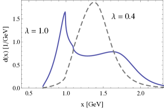
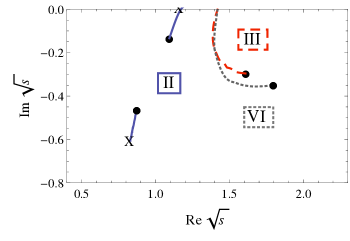
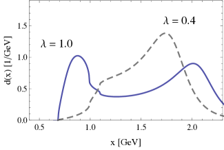
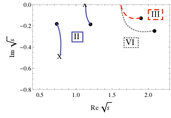
   Figure 1: Spectral functions (left panels) and positions of poles in the complex $\sqrt{s}$-plane (right panels) for the parameter sets of TR (upper row) and BP (lower row). Spectral functions are shown for $\lambda=0.4$ (dashed grey lines) and $\lambda=1.0$ (solid blue lines). The pole trajectories of the seed state are indicated by grey dotted or red dashed lines (for details, see the text) and the one for the dynamically generated resonance by solid blue lines. The roman numerals indicate the Riemann sheets where the respective poles can be found. Final pole positions $(\lambda=1.0)$ are indicated by solid black dots, pole positions at $\lambda_{c,i}$, i.e., where the pole $i$ first emerges, are indicated by X.

   However, we also find another pole on the second sheet emerging at a large imaginary value of $\sqrt{s}$ and moving up towards the real axis. It first appears for $\lambda_{c,2}^{\text{TR}}\approx 0.84$. Its effect on the spectral function is hard to discern, since (the absolute value of) its imaginary part (i.e., its decay width) is still too large at $\lambda=1.0$. This pole was not reported in TR, yet, in Ref. van Beveren and Rupp (1999), a similar situation was described where the $a_{0}(980)$ was taken to have such a behavior, i.e., its pole was coming from the region of large negative imaginary parts of $\sqrt{s}$ and heading towards the real axis. This is, however, not the case for the pole of TR, which is dynamically generated near the real axis and then shifts towards larger (negative) imaginary values of $\sqrt{s}$.

   On the third sheet, TR reports another pole. One could think that this pole corresponds to the seed state, since for $\lambda=0$ the pole trajectory starts on the real axis at the mass of the seed state. However, the pole lies on the third sheet, i.e., prior to crossing the $\pi\eta^{\prime}$-threshold, but its location is above that threshold. Therefore, it should not be considered to induce the broad bump in the spectral function. However, there is also a pole on the sixth sheet which also starts at the mass of the seed state. From its position this pole can also be considered to generate the broad resonance shape in the spectrum above $1.5$ GeV. It is interesting that the pole on the third sheet was suggested in TR to correspond to the $a_{0}(1450)$ resonance. From our point of view, because of the above arguments it is more natural to take the pole on the sixth sheet. A close inspection of the peak position of the broad bump in the spectral function reveals that it corresponds more closely to the real part of the pole on the sixth sheet than that on the third sheet, which corroborates our interpretation.

2. In the lower row of Fig. 1 we present the results for the parameter choice in BP. We find that the qualitative behavior is very similar to the one in TR. Quantitatively, we find that the bump in the spectral function corresponding to the $a_{0}(980)$ resonance is now somewhat wider. The broad structure at large $\sqrt{s}$ is more pronounced and now lies around $2$ GeV. For decreasing coupling strength the peak becomes narrower and moves towards $1.6$ GeV (because the seed state is located there).

   We find again two poles on the second sheet. The right pole appears first for $\lambda_{c,1}^{\text{BP}}\approx 0.69$ and the left one for $\lambda_{c,2}^{\text{BP}}\approx 0.66$. The parameter set of BP does not yield a pole structure from which one can infer which pole corresponds to the $a_{0}(980)$. Both poles give too large widths, and the left one is too light, while the right one is too heavy. It seems that both of them are relevant in the generation of the bump at $1$ GeV in the spectrum. Moreover, it does not seem to be appropriate to assign the poles on the other two sheets to $a_{0}(1450)$. At least within this model and with the chosen parameters, the pole masses are definitely too high .

III Simple effective model with derivative interactions

In the previous section we have re-examined the approach of TR and BP to dynamically generate resonances in the scalar–isovector sector. We now apply the above mechanism of dynamical generation of resonances using a formulation based on an interaction Lagrangian.

III.1 Interactions with derivatives: a lesson from the eLSM

The way a scalar field couples to pseudoscalar states depends on the effective approach used. Let us, for instance, consider the coupling of $a_{0}$ to kaons. In chiral perturbation theory (chPT) Gasser and Leutwyler (1984); *[seealso][andrefs.therein]chpt2, which is based on the nonlinear realization of chiral symmetry, only derivative couplings of the type $a_{0}^{0}\partial_{\mu}K^{0}\partial^{\mu}\bar{K}^{0}$ can appear in the chiral limit Ecker et al. (1989). Away from the chiral limit, a non-derivative coupling $a_{0}^{0}K^{0}\bar{K}^{0}$ appears, too, but its strength is proportional to $m_{K}^{2}$, i.e., via the Gell-Mann–Oakes–Renner relation proportional to the explicit breaking of chiral symmetry by nonzero quark masses. On the other hand, if the standard linear sigma model (without vector degrees of freedom) is considered, the coupling is only of the non-derivative type $a_{0}^{0}K^{0}\bar{K}^{0}$. At tree-level both chPT and the sigma model can coincide, but when loops are included differences arise due to the different $s$-dependence in the amplitudes.

Studying the spectral function of $\phi\rightarrow a_{0}(980)\gamma\rightarrow\pi^{0}\eta\gamma$ measured by the KLOE Collaboration Ambrosino et al. (2007), it was shown in Ref. Giacosa and Pagliara (2008); *pagliaraderivatives2 that a derivative coupling of the type $a_{0}^{0}\partial_{\mu}K^{0}\partial^{\mu}\bar{K}^{0}$ seems to be necessary. As we shall demonstrate below, we come to the same conclusion: a derivative coupling is necessary for the simultaneous description of both resonances $a_{0}(980)$ and $a_{0}(1450)$.

Interestingly, an improved version of the linear sigma model, called extended Linear Sigma Model (eLSM), naturally contains both non-derivative and derivative coupling terms. This feature is due to the inclusion of (axial-)vector degrees of freedom in the model, for more details see Refs. Gallas et al. (2010); *eLSM1-2; *eLSM1-3; Parganlija et al. (2013). This model is able to provide a surprisingly good description of the tree-level masses and decay widths of meson resonances below $1.7$ GeV Gallas et al. (2010); *eLSM1-2; *eLSM1-3; Parganlija et al. (2013); Janowski et al. (2014). Furthermore, in this approach the resonance $a_{0}(1450)$ turns out to be predominantly a quark-antiquark state with a (bare) mass of $m_{a_{0}}=1.363$ GeV.

The Lagrangian for the scalar–isovector sector emerging from the eLSM has the following form:

$$\mathcal{L}_{a_{0}\eta\pi}^{\text{eLSM}} = A_{1}^{\text{eLSM}}a_{0}^{0}\eta\pi^{0}+B_{1}^{\text{eLSM}}a_{0}^{0}\partial_{\mu}\eta\partial^{\mu}\pi^{0}+C_{1}^{\text{eLSM}}\partial_{\mu}a_{0}^{0}(\pi^{0}\partial^{\mu}\eta+\eta\partial^{\mu}\pi^{0})\ ,$$ (10)

$$\mathcal{L}_{a_{0}\eta^{\prime}\pi}^{\text{eLSM}} = A_{2}^{\text{eLSM}}a_{0}^{0}\eta^{\prime}\pi^{0}+B_{2}^{\text{eLSM}}a_{0}^{0}\partial_{\mu}\eta^{\prime}\partial^{\mu}\pi^{0}+C_{2}^{\text{eLSM}}\partial_{\mu}a_{0}^{0}(\pi^{0}\partial^{\mu}\eta^{\prime}+\eta^{\prime}\partial^{\mu}\pi^{0})\ ,$$

$$\mathcal{L}_{a_{0}K\bar{K}}^{\text{eLSM}} = A_{3}^{\text{eLSM}}a_{0}^{0}(K^{0}\bar{K}^{0}-K^{-}K^{+})+B_{3}^{\text{eLSM}}a_{0}^{0}(\partial_{\mu}K^{0}\partial^{\mu}\bar{K}^{0}-\partial_{\mu}K^{-}\partial^{\mu}K^{+})$$

$$+\ C_{3}^{\text{eLSM}}\partial_{\mu}a_{0}^{0}(K^{0}\partial^{\mu}\bar{K}^{0}+\bar{K}^{0}\partial^{\mu}K^{0}-K^{-}\partial^{\mu}K^{+}-K^{+}\partial^{\mu}K^{-})\ ,$$

where $A_{i}^{\text{eLSM}}$, $B_{i}^{\text{eLSM}}$, and $C_{i}^{\text{eLSM}}$ are coupling constants that are functions of the parameters of the model Parganlija et al. (2013). Note that both non-derivative and derivative interactions appear. The derivatives in front of the fields produce an $s$-dependence in the decay amplitudes, $-i\mathcal{M}_{i}^{\text{eLSM}}(s)$, which enter the tree-level expressions of the decay widths,

$$\Gamma_{i}^{\text{eLSM}}(s)=\frac{k_{i}(s)}{8\pi s}|\text{--}i\mathcal{M}_{i}^{\text{eLSM}}(s)|^{2}\Theta(s-s_{th,i})\ ,$$ (11)

which have to be evaluated for $s=m_{a_{0}}^{2}$. The amplitudes read

$$\mathcal{M}_{i}^{\text{eLSM}}(s)=A_{i}^{\text{eLSM}}-\frac{1}{2}B_{i}^{\text{eLSM}}\left(s-m_{i1}^{2}-m_{i2}^{2}\right)+C_{i}^{\text{eLSM}}s\ ,$$ (12)

where the masses $m_{i1},m_{i2}$ are the pseudoscalar masses in the relevant channels. The parameters of the eLSM were determined from a $\chi^{2}$-fit to tree-level masses and decay widths. So far, no loop corrections were considered. For a consistent loop calculation one would have to perform a new fit of the parameters, which is an interesting project for future work. In any case, one should not use the values of the parameters of the eLSM determined in Ref. Parganlija et al. (2013) in the expressions for $A_{i}^{\text{eLSM}},B_{i}^{\text{eLSM}}$, and $C_{i}^{\text{eLSM}}$. Therefore, we shall treat the latter as free parameters in the following.

A first attempt to incorporate loop corrections in a scheme inspired by the eLSM was presented in Refs. Wolkanowski (2015); Wolkanowski and Giacosa (2014). There, the $s$-dependence of the amplitudes was completely neglected and a regularization function was introduced,

$$-i\mathcal{M}_{i}^{\text{eLSM}}(s)\ \rightarrow\ -i\mathcal{M}_{i}(s)=-i\mathcal{M}_{i}^{\text{eLSM}}(m_{a_{0}}^{2})F_{i}(s)\ .$$ (13)

After that, the imaginary part of the self-energy was computed using the optical theorem,

$$\operatorname{Im}\Pi_{i}(s)=-\sqrt{s}\,\Gamma_{i}^{\text{tree}}(s)=-\frac{k_{i}(s)}{8\pi\sqrt{s}}|\text{--}i\mathcal{M}_{i}(s)|^{2}\Theta(s-s_{th,i})\ ,$$ (14)

and the real part from the dispersion relation (2). As shown in Ref. Wolkanowski (2015) the model yields a width of the seed state which is too small. Moreover, no additional pole for the $a_{0}(980)$ is dynamically generated. Obviously, neglecting the $s$-dependence of the amplitudes is an oversimplification. One has to take into account the derivatives in some way; at the same time care is needed when derivative interactions appear in a Lagrangian, for details see App. A.

III.2 Effective model with both non-derivative and derivative interactions

We now consider an effective model for the isovector states containing the same decay channels as the eLSM and including also non-derivative and derivative interactions. The Lagrangian is given by the sum of the following terms:

$$\mathcal{L}_{a_{0}\eta\pi} = A_{1}a_{0}^{0}\eta\pi^{0}+B_{1}a_{0}^{0}\partial_{\mu}\eta\partial^{\mu}\pi^{0}\ ,$$ (15)

$$\mathcal{L}_{a_{0}\eta^{\prime}\pi} = A_{2}a_{0}^{0}\eta^{\prime}\pi^{0}+B_{2}a_{0}^{0}\partial_{\mu}\eta^{\prime}\partial^{\mu}\pi^{0}\ ,$$

$$\mathcal{L}_{a_{0}K\bar{K}} = A_{3}a_{0}^{0}(K^{0}\bar{K}^{0}-K^{-}K^{+})+B_{3}a_{0}^{0}(\partial_{\mu}K^{0}\partial^{\mu}\bar{K}^{0}$$

$$-\ \partial_{\mu}K^{-}\partial^{\mu}K^{+})\ .$$

Formally it can be obtained by rewriting the terms proportional to $C_{i}^{\text{eLSM}}$ in Eq. (10) by an integration by parts in order to get rid of the derivatives of the $a_{0}$-fields . Subsequently, one replaces the emerging second derivatives with the help of the Klein–Gordon equation, $\square\pi^{0}=-m_{\pi}^{2}\pi^{0}$ (and similarly for the other pseudoscalar fields). Then, Eq. (15) gives rise to the following $s$-dependent amplitudes:

$$\mathcal{M}_{i}^{\text{eff}}(s)=\left[A_{i}-\frac{1}{2}B_{i}\left(s-m_{i1}^{2}-m_{i2}^{2}\right)\right]F_{i}(s)\ ,$$ (16)

where we have already included a regularization function $F_{i}(s)$ as defined in Sec. II. We again note that the constants $A_{i}$ and $B_{i}$ will not be computed from the numerically determined parameters of the eLSM, but will be determined in order to produce the masses and decay widths of the resonances under study. Note that in chPT the parameters $A_{i}$ are proportional to the masses of the pseudo-Goldstone bosons as $A_{1}\propto m_{\pi}^{2}+m_{\eta}^{2}$, $A_{2}\propto m_{\pi}^{2}+m_{\eta^{\prime}}^{2}$, $A_{3}\propto 2m_{K}^{2}$ and thus vanish in the chiral limit. Thus, also from this consideration, we expect that the derivative terms are sizable and crucial for the determination of the resonance poles.

We computed the real and imaginary part of the self-energy in two ways. In the first, we applied the method outlined in Sec. III.1, i.e., we computed the tree-level decay widths and used the optical theorem from Eq. (14) to obtain the imaginary part of the self-energy. We then applied the dispersion relation (2) to calculate the corresponding real part. In the second approach, we computed the one-loop self-energy directly from the Feynman rules. From a comparison, we identified the necessity to introduce subtractions in the first approach, for details see App. A. Note that the one-loop approximation for the self-energy is quite reliable, since vertex corrections can be shown to have a negligible effect Schneitzer et al. (2014).

There are eight parameters in our approach: $m_{0},\ \Lambda=\sqrt{2}k_{0},$ and six coupling constants $A_{i},B_{i}$ $(i=1,2,3)$. We vary the numerical values of $m_{0}$ and $\Lambda$ within reasonable intervals $m_{0}\in(0.8,1.5)$ GeV and $\Lambda\in(0.4,1.5)$ GeV and each time perform a fit of the six coupling constants to six experimental quantities: one pole in the PDG range for $a_{0}(980)\ (\text{in our case }\sqrt{s}=(0.969-i\hskip 0.56917pt0.045)\ \text{GeV})$ and one for $a_{0}(1450)\ (\text{in our case }\sqrt{s}=(1.450-i\hskip 0.56917pt0.135)\ \text{GeV})$, and the central values of the branching ratios of $a_{0}(1450)$ [see Eq. (22)]. By this, all six free parameters can be fixed.

It turns out that there is only a narrow range of suitable values of the parameters $m_{0}$ and $\Lambda$ for which the fit of the six coupling constants is possible: approximately $m_{0}\in(0.9,1.2)$ GeV and $\Lambda\in(0.4,0.9)$ GeV. Here, ‘approximately’ refers to the fact that, due to the interdependence of the parameters, the window is not rectangular. However, a small change in $m_{0}$ and/or $\Lambda$ by 50 MeV near the borders of the quoted interval does not allow one to reproduce the data anymore. Thus, although we have eight parameters, we are severely constrained in their choice in order to describe the $I=1$ resonance. As we will see below, the present parameters also explain why $a_{0}(980)$ couples strongly to kaons. The final values for the parameters and coupling constants are:

$$m_{0} =1.15\ \text{GeV}\ , \Lambda =0.6\ \text{GeV}\ ,$$ (17)

$$A_{1} =2.52\ \text{GeV}\ , B_{1} =-8.07\ \text{GeV}^{-1}\ ,$$ (18)

$$A_{2} =9.27\ \text{GeV}\ , B_{2} =9.25\ \text{GeV}^{-1}\ ,$$

$$A_{3} =-6.56\ \text{GeV}\ , B_{3} =-1.54\ \text{GeV}^{-1}\ .$$

We rescale these coupling constants by a common factor $\sqrt{\lambda}$ and compute the corresponding spectral functions. The result is shown in the left panel of Fig. 2. We also compute the pole trajectories in the complex $\sqrt{s}$-plane by varying $\lambda$ from zero to one.

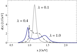
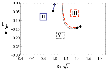
Figure 2: In the left panel we show the spectral functions for three different values of $\lambda$. In the right panel we display pole trajectories obtained by varying $\lambda$ from zero to one. Black dots indicate the position of the poles for $\lambda=1.0$. The X indicates the pole position for $\lambda_{c}$, i.e., when the pole first emerges. The roman numeral indicates on which sheet the respective pole can be found.

The following comments are in order:

1. The spectral function shows a narrow peak for $\lambda=1.0$ at a value of $x=\sqrt{s}$ slightly smaller than $1$ GeV, which can be interpreted as the $a_{0}(980)$. The form is distorted by the nearby $K\bar{K}$-threshold and resembles the Flatté distribution Flatté (1976a); *flatte2, see also Refs. Giacosa and Pagliara (2007); Baru et al. (2005) and refs. therein. The pole corresponding to this peak lies on the second sheet and has coordinates

   $$\sqrt{s}=(0.970-i\hskip 0.56917pt0.045)\ \text{GeV}\ ,$$ (19)

   i.e., we find the $a_{0}(980)$ to have a mass of $m_{\text{pole}}=0.969$ GeV and a width of $\Gamma_{\text{pole}}=0.090$ GeV. This pole appears only if $\lambda$ exceeds $\lambda_{c}\approx 0.52$ (note that the pole trajectory is very different from the one reported in Ref. Zhou and Xiao (2011)). The corresponding position is indicated by an X in the right panel of Fig. 2. The important thing here is that, in contrast to what we have found for the TR and BP parametrizations, there is only one pole for the $a_{0}(980)$, and thus no ambiguity which one should be identified with this resonance .

2. There is also a broad structure around $1.5$ GeV which corresponds to the resonance $a_{0}(1450)$. For decreasing $\lambda$, both peaks merge and settle around $1.15$ GeV, where the seed state is located.

3. As expected, there is (only) one pole present on the third sheet with coordinates $\sqrt{s}=(1.400-i\hskip 0.56917pt0.141)$ GeV. However, as in TR and BP, we find a pole on the sixth sheet, too. Its coordinates are

   $$\sqrt{s}=(1.456-i\hskip 0.56917pt0.134)\ \text{GeV}\ ,$$ (20)

   or $m_{\text{pole}}=1.450$ GeV and $\Gamma_{\text{pole}}=0.270$ GeV. This is the pole which is responsible for the peak around $1.5$ GeV in the spectrum, and thus we assign it to the $a_{0}(1450)$. However, since the pole on the third sheet also reproduces mass and width of $a_{0}(1450)$ to reasonable accuracy, it is in principle possible to regard this one as the pole corresponding to $a_{0}(1450)$, too.

The present study demonstrates that, by starting with a unique seed state, it is indeed possible to find two poles for the isovector states, both of which reproduce the masses and widths of $a_{0}(980)$ and $a_{0}(1450)$ reasonably well.

III.3 Branching ratios and coupling constants for $a_{0}(980)$

For completeness, we report the branching ratios of our effective model by using the tree-level decay widths obtained from the optical theorem (14). The partial widths are evaluated at the peak value of the spectral function above $1$ GeV, $m_{\text{peak}}=1.419$ GeV. For the resonance $a_{0}(1450)$ this leads to

$$\frac{\Gamma_{a_{0}\rightarrow\eta^{\prime}\pi}^{\text{tree}}}{\Gamma_{a_{0}\rightarrow\eta\pi}^{\text{tree}}}\simeq 0.44\ ,\ \ \ \frac{\Gamma_{a_{0}\rightarrow K\bar{K}}^{\text{tree}}}{\Gamma_{a_{0}\rightarrow\eta\pi}^{\text{tree}}}\simeq 0.96\ ,$$ (21)

which can be compared to the experimental values Olive et al. (2014):

$$\frac{\Gamma_{a_{0}\rightarrow\eta^{\prime}\pi}}{\Gamma_{a_{0}\rightarrow\eta\pi}}=0.35\pm 0.16\ ,\ \ \ \frac{\Gamma_{a_{0}\rightarrow K\bar{K}}}{\Gamma_{a_{0}\rightarrow\eta\pi}}=0.88\pm 0.23\ .$$ (22)

Concerning the resonance $a_{0}(980)$, we give the following estimates for the coupling constants in the $\pi\eta$- and $K\bar{K}$-channels: We calculate the partial widths $\Gamma_{i}^{\text{tree}}(s)$, this time with $\sqrt{s}$ equal to the peak mass of the spectral function below $1$ GeV, $m_{\text{peak}}=0.956$ GeV. Then, Eq. (14) is used to solve for the absolute values of the amplitudes. The result is multiplied with the root of the wave-function renormalization factor, $\sqrt{Z}=0.652$, which is its value at the Breit–Wigner mass of the $a_{0}(980)$. Thus we obtain the coupling constants in the $\pi\eta$- and $K\bar{K}$-channels as

$$g_{\pi\eta}=2.496\ \text{GeV}\ ,\ \ \ g_{K\bar{K}}=6.012\ \text{GeV}\ .$$ (23)

It is remarkable that the coupling of $a_{0}(980)$ to kaons turns out to be sizably larger than the coupling to $\pi\eta$. This is in agreement with various other works on this topic Krehl and Speth (1997); *molecular2; *molecular3; *molecular4; *molecular5; Giacosa and Pagliara (2008); *pagliaraderivatives2; Maiani et al. (2004): Virtual kaon-kaon pairs near the kaon-kaon threshold are important for the dynamical generation of the resonance $a_{0}(980)$.

IV Conclusions

$a_{0}(980)$			$a_{0}(1450)$
	$m_{\text{pole}}$ [GeV]	$\Gamma_{\text{pole}}$ [GeV]	$m_{\text{pole}}$ [GeV]	$\Gamma_{\text{pole}}$ [GeV]
TR Törnqvist (1995); *tornqvist2	$1.084$	$0.270$	$1.566$	$0.578$
BP Boglione and Pennington (2002)	$1.186$*	$0.373$*	$1.896$	$0.250$
Our results	$0.969$	$0.090$	$1.450$	$0.270$
PDG Olive et al. (2014)	$\ 0.980\pm 0.020\$	$\ 0.050$ to $0.100$	$\ 1.474\pm 0.019\$	$\ 0.265\pm 0.013$
*In order to compare to TR, the right pole on the second sheet was chosen.

Table 1: Numerical results for the pole coordinates in the scalar–isovector sector in TR, BP, and our effective model, compared to the PDG values. In the case of the $a_{0}(1450)$, the poles listed for TR and BP are located on the third sheet, while our pole lies on the sixth sheet. All poles for the $a_{0}(980)$ are found on the second sheet. Note that all poles listed for BP were obtained performing the analytic continuation of the propagator given by BP.

Experimental data exhibit several puzzling facts about the light scalar mesons: $f_{0}(500)$ (or $\sigma$) and $K_{0}^{\ast}(800)$ have large decay widths, while $f_{0}(980)$ and $a_{0}(980)$ are narrow but their spectral functions show threshold distortions due to the nearby $K\bar{K}$-threshold. It is nowadays recognized that these states do not fit into the ordinary $q\bar{q}$ picture based on a simple representation of $SU(3)$–flavour symmetry Godfrey and Isgur (1985), yet there is no consensus on the precise mechanism which generates them. One can also regard these states as four-quark objects, for example as tetraquarks Jaffe (1977a); *jaffe2; Maiani et al. (2004); Fariborz (2004); *fariborz2; Napsuciale and Rodriguez (2004); Giacosa (2007) or as dynamically generated states. The latter are states which are not present in the original formulation of a hadronic model but appear when calculating loop corrections Oller and Oset (1997); *oller2; *oller3; Peláez and Ríos (2006); *pelaez2; van Beveren et al. (1986); Törnqvist (1995); *tornqvist2; Morgan and Pennington (1993); Boglione and Pennington (1997). Indeed, the interpretation of light scalar states as loosely bound molecular states Krehl and Speth (1997); *molecular2; *molecular3; *molecular4; *molecular5 is also an example of dynamical generation. [For another interpretation of light scalar states, see e.g. Ref. Minkowski and Ochs (2005); *ochs2; *ochs3.]

A particular type of dynamical generation is that of ‘image’ or ‘companion poles’. We have concentrated on such a method in this work and have applied it to the scalar–isovector sector. Our results demonstrate that it is in fact possible to correctly describe the resonances $a_{0}(980)$ and $a_{0}(1450)$ in a unique framework, where originally only a single quark-antiquark seed state is present.

Besides that, we have also repeated the previous calculations of Törnqvist and Roos Törnqvist (1995); *tornqvist2 and Boglione and Pennigton Boglione and Pennington (2002). These studies have been extended by us to the complex plane on all Riemann sheets nearest to the first, physical sheet. A summary of our results and, for comparison, those of Törnqvist and Roos, and Boglione and Pennington, can be found in Tab. 1. Our results are based on an effective Lagrangian approach that includes both derivative and non-derivative interaction terms, see Eq. (15), inspired by the extended Linear Sigma Model (eLSM), and show that both terms are necessary and equally important Gallas et al. (2010); *eLSM1-2; *eLSM1-3; Parganlija et al. (2013).

Note that the formulation of dynamical generation applied here is related, but not equal to the one described in Ref. Oller and Oset (1997); *oller2; *oller3. In the latter the scattering amplitude is computed from an effective Lagrangian (derived from chiral perturbation theory and containing only pseudoscalar mesons) and then unitarized; this process of unitarization generates, for instance, the pole of the $a_{0}(980)$ in the scalar–isovector sector. Yet, it is $a\ priori$ not possible to know if the resulting state is in fact a quark-antiquark or a four-quark resonance, and if it can be linked to the heavier $a_{0}(1450)$ state or not; see Ref. Giacosa (2009) for a detailed discussion of this issue. However, further studies within this scheme were performed in Ref. Oller and Oset (1999) by including an octet of bare resonances masses around $1.4$ GeV. It was found that the physical $a_{0}(1450)$ in fact originates from this octet, giving a clear statement about its nature, which is in agreement with our results.

In this work we have concentrated on the isovector sector $I=1.$ However, the very same mechanism is applicable for the other light and heavy scalar states. As a consequence, all light scalars are dynamically generated states. In particular, it seems promising to extend the present study in the low-energy regime into two directions: $(i)$ The isodoublet, i.e., by describing the resonances $K_{0}^{\ast}(800)$ and $K_{0}^{\ast}(1430)$ in a similar framework. The pole of $K_{0}^{\ast}(800)$ is not yet very well known and there is need of improved analyses from different directions. $(ii)$ The scalar–isoscalar sector, where the resonances $f_{0}(500)$ and $f_{0}(980)$ should be dynamically generated. In this case, $f_{0}(1370),$ $f_{0}(1500)$, and $f_{0}(1710)$ would be predominantly a non-strange quarkonium, a strange quarkonium, and a scalar glueball, respectively.

Another interesting subject is the study of dynamical generation in the framework of puzzling resonances in the charmonium sector Pennington and Wilson (2007), see for example Ref. Brambilla et al. (2011) and refs. therein. Namely, a whole class of mesons, called $X$, $Y$, and $Z$ states, has been experimentally discovered but is so far not fully understood Braaten et al. (2014); *braaten2; Maiani et al. (2007). As demonstrated in Ref. Coito et al. (2013) for the case of $X(3872)$, some of the $X$ and $Y$ states could emerge as companion poles of quark-antiquark states.

Appendix A

In this Appendix, we compute the one-loop self-energy in the case of derivative interactions. We first derive the interacting part of the Hamiltonian from the Lagrangian via a Legendre transformation. We shall see that the derivative interactions give rise to new interaction vertices. We demonstrate that, in a perturbative calculation of the one-loop self-energy, these terms are necessary to cancel additional terms arising from contractions of gradients of fields. This proves that, at least at the one-loop level, it is justified to apply standard Feynman rules with the derivative interaction in ${\cal L}_{\text{int}}$. We shall also demonstrate that a computation of the self-energy via the dispersion relation (2) may require subtraction constants to agree with the perturbative calculation using Feynman rules.

Canonical quantization

Let us consider a theory with two scalar fields, $S$ and $\phi$, which allows for the decay process $S\rightarrow\phi\phi$. Consequently, the Lagrangian is

$$\mathcal{L}=\mathcal{L}_{S}+\mathcal{L}_{\phi}+\mathcal{L}_{\text{int}}\;,$$ (24)

where

$$\mathcal{L}_{S} = \frac{1}{2}\left(\partial_{\mu}S\partial^{\mu}S-M^{2}S^{2}\right)\;,$$

$$\mathcal{L}_{\phi} = \frac{1}{2}\left(\partial_{\mu}\phi\partial^{\mu}\phi-m^{2}\phi^{2}\right)\;,$$

$$\mathcal{L}_{\text{int}} = gS\partial_{\mu}\phi\partial^{\mu}\phi\;.$$ (25)

For perturbative calculations of $\hat{S}$-matrix elements or Green’s functions, however, one needs the interaction part of the Hamilton operator in the interaction picture. We derive this operator via a Legendre transformation of ${\cal L}$ and subsequent canonical quantization in the interaction picture. As a byproduct of this calculation we will explicitly show that the derivative interactions invalidate the commonly used relation $\mathcal{H}_{\text{int}}=-\mathcal{L}_{\text{int}}$ Greiner and Reinhardt (1996).

The canonically conjugate fields are

$$\pi_{S} = \frac{\partial\mathcal{L}}{\partial(\partial_{0}S)}=\partial^{0}S\ ,$$ (26)

$$\pi_{\phi} = \frac{\partial\mathcal{L}}{\partial(\partial_{0}\phi)}=\partial^{0}\phi+2gS\partial^{0}\phi=(1+2gS)\partial^{0}\phi\ .$$

The Hamiltonian is defined via a Legendre transformation of ${\cal L}$,

$$\mathcal{H} = \pi_{S}\partial^{0}S+\pi_{\phi}\partial^{0}\phi-\mathcal{L}$$

$$= \frac{1}{2}\pi_{S}\pi_{S}+\frac{1}{2}\vec{\nabla}S\cdot\vec{\nabla}S+\frac{1}{2}M^{2}S^{2}+\frac{1}{2}\pi_{\phi}\pi_{\phi}(1+2gS)^{-1}$$

$$+\ \frac{1}{2}\vec{\nabla}\phi\cdot\vec{\nabla}\phi+\frac{1}{2}m^{2}\phi^{2}+gS\vec{\nabla}\phi\cdot\vec{\nabla}\phi\ .$$

For a perturbative calculation, we need to expand the denominator $(1+2gS)^{-1}$ and obtain the interaction part of the Hamiltonian as

$$\mathcal{H}_{\text{int}}=-gS\pi_{\phi}\pi_{\phi}+gS\vec{\nabla}\phi\cdot\vec{\nabla}\phi+2g^{2}S^{2}\pi_{\phi}\pi_{\phi}+\mathcal{O}(g^{3})\ .$$ (28)

We may now quantize in the Heisenberg picture (indicated by a superscript $H$ at the respective operators). This is commonly done by promoting fields to operators $S\rightarrow\hat{S}^{H}$, $\phi\rightarrow\hat{\phi}^{H}$, $\pi_{S}\rightarrow\hat{\pi}_{S}^{H}$, $\pi_{\phi}\rightarrow\hat{\pi}_{\phi}^{H}$, and postulating certain commutation relations for these operators. However, in perturbation theory we need the operators in the interaction picture. The following relations hold,

$$\hat{S}^{I} =\hat{U}\hat{S}^{H}\hat{U}^{\dagger}\ , \hat{\phi}^{I} =\hat{U}\hat{\phi}^{H}\hat{U}^{\dagger}\ ,$$ (29)

$$\hat{\pi}_{S}^{I} =\hat{U}\hat{\pi}_{S}^{H}\hat{U}^{\dagger}\ , \hat{\pi}_{\phi}^{I} =\hat{U}\hat{\pi}_{\phi}^{H}\hat{U}^{\dagger}\ ,$$

where $\hat{U}=e^{i\hat{H}_{0}t}e^{-i\hat{H}t}$ is the time-evolution operator that relates operators in the Heisenberg picture with those in the interaction picture. Finally, replacing $\hat{\pi}^{I}_{S}=\partial^{0}\hat{S}^{I},\,\hat{\pi}^{I}_{\phi}=\partial^{0}\hat{\phi}^{I}$ this results in

$$\hat{\mathcal{H}}_{\text{int}}^{I}=-\hat{\mathcal{L}}_{\text{int}}^{I}+2g^{2}\hat{S}^{I}\hat{S}^{I}\partial_{0}\hat{\phi}^{I}\partial^{0}\hat{\phi}^{I}+\mathcal{O}(g^{3})\ .$$ (30)

As advertised, the second term spoils the standard relation $\hat{\mathcal{H}}_{\text{int}}=-\hat{\mathcal{L}}_{\text{int}}$. This term corresponds to a four-point vertex, so it will not appear in the tree-level decay $S\rightarrow\phi\phi$. In contrast, in the one-loop self-energy, it will give rise to an additional tadpole contribution.

Perturbative calculation of the one-loop self-energy

We now turn to the self-energy $\Pi(s)$ of the field $S$. At one-loop level, the Feynman rules applied to $\hat{\cal H}_{\text{int}}$ tell us that we will have two contributions. The first contribution comes from taking two three-point vertices of $\hat{\cal L}_{\text{int}}$ where the $\hat{\phi}$ legs are joined in a manner which gives a 1PI diagram. A covariant derivative acts on each $\hat{\phi}$ leg at each vertex. The second contribution is a tadpole term arising from the four-point vertex in Eq. (30), which has two time derivatives on the internal leg. This can be graphically depicted as follows:

(31)

The usual Feynman propagator is defined as a contraction of two fields:

$$\bcontraction{}{\hat{\phi}}{(x_{1})}{\hat{\phi}}\hat{\phi}(x_{1})\hat{\phi}(x_{2}) = \langle 0|\mathcal{T}\big{\{}\hat{\phi}(x_{1})\hat{\phi}(x_{2})\big{\}}|0\rangle$$

$$= \langle 0|\hat{\phi}(x_{1})\hat{\phi}(x_{2})|0\rangle\Theta(x_{1}^{0}-x_{2}^{0})$$

$$+\ \langle 0|\hat{\phi}(x_{2})\hat{\phi}(x_{1})|0\rangle\Theta(x_{2}^{0}-x_{1}^{0})$$

$$= i\Delta_{F}^{\phi}(x_{1}-x_{2})$$

$$= i\int\frac{\text{d}^{4}p}{(2\pi)^{4}}\frac{e^{-ip\cdot(x_{1}-x_{2})}}{p^{2}-m^{2}+i\epsilon}\ .$$

However, in the tadpole diagram, we have the contraction of two fields on each of which acts a time derivative. Because time-ordering has no effect at the same space-time point, we obtain:

$$\langle 0|\mathcal{T}\big{\{}\partial_{0}^{x}\hat{\phi}(x)\partial^{0,x}\hat{\phi}(x)\big{\}}|0\rangle = \langle 0|{}\partial_{0}^{x}\hat{\phi}(x)\partial^{0,x}\hat{\phi}(x)|0\rangle$$

$$= i\int\frac{\text{d}^{4}p}{(2\pi)^{4}}\frac{E_{\textbf{p}}^{2}}{p^{2}-m^{2}+i\epsilon}\ .$$

In order to obtain this result we inserted the standard Fourier decomposition of the field operators

$$\hat{\phi}(x)=\int\frac{\text{d}^{3}p}{(2\pi)^{3}}\frac{1}{\sqrt{2E_{\textbf{p}}}}\Big{(}\hat{a}_{\textbf{p}}^{\dagger}e^{ip\cdot x}+\hat{a}_{\textbf{p}}e^{-ip\cdot x}\Big{)}\;,$$ (34)

where $p^{0}=E_{\bf p}=\sqrt{{\bf p}^{2}+m^{2}}$ is the on-shell energy. Thus, a time derivative acting on a field operator brings down a factor of $\pm i$ times the on-shell energy in the corresponding Fourier representation.

The result (A) is, however, identical if we just act with the time derivatives on the standard Feynman propagator (A):

$$\partial_{0}^{x}\partial^{0,x}\langle 0|{}\hat{\phi}(x)\hat{\phi}(x)|0\rangle = \lim_{x_{1}\rightarrow x_{2}}\partial_{0}^{x_{1}}\partial^{0,x_{2}}\langle 0|\mathcal{T}\big{\{}\hat{\phi}(x_{1})\hat{\phi}(x_{2})\big{\}}|0\rangle$$ (35)

$$= i\int\frac{\text{d}^{4}p}{(2\pi)^{4}}\frac{E_{\textbf{p}}^{2}}{p^{2}-m^{2}+i\epsilon}\ .$$

In order to prove this, it is convenient to first perform the $p_{0}$ integration in Eq. (A) and then take the time derivatives. The equivalence of Eqs. (A) and (35) is graphically depicted as

$$\langle 0|\mathcal{T}\big{\{}\partial_{0}^{x}\phi (x)\partial^{0,x}\phi(x)\big{\}}|0\rangle\ \ \sim$$

In the perturbative series of the full propagator of the $S$-field, this tadpole contribution appears in combination with two free $S$-field propagators (where we omit the superscript $S$):

$$\frac{-2\hskip 0.28436pti\hskip 0.28436ptg^{2}}{1!}\cdot 2\int\text{d}x^{\prime}\ i\Delta(x_{1}-x^{\prime})\langle 0|\mathcal{T}\big{\{}\partial_{0}^{x^{\prime}}\phi(x^{\prime})\partial^{0,x^{\prime}}\phi(x^{\prime})\big{\}}|0\rangle\hskip 0.56917pti\Delta(x^{\prime}-x_{2})$$ (37)

$$=\ i\hskip 0.56917pt2g^{2}\cdot 2\int\text{d}x^{\prime}\ \Delta(x_{1}-x^{\prime})\Delta(x^{\prime}-x_{2})\langle 0|\mathcal{T}\big{\{}\partial_{0}^{x^{\prime}}\phi(x^{\prime})\partial^{0,x^{\prime}}\phi(x^{\prime})\big{\}}|0\rangle\ .$$

The factor $-2ig^{2}$ is the factor accompanying the four-point vertex, cf. Eq. (30). A factor of two arises because each $S$ propagator can be joined with either one of the $S$ legs at the vertex.

We now compute the first diagram in Eq. (31). To this end, we need contractions of gradients of the $\phi$-fields. These can be expressed in terms of gradients acting on the standard Feynman propagator. The gradient of the Feynman propagator (A) is

$$i\hskip 0.56917pt\partial_{\nu}^{x_{2}}\Delta_{F}^{\phi}(x_{1}-x_{2}) = \partial_{\nu}^{x_{2}}\langle 0|\mathcal{T}\big{\{}\phi(x_{1})\phi(x_{2})\big{\}}|0\rangle$$

$$= \langle 0|\mathcal{T}\big{\{}\phi(x_{1})\partial_{\nu}^{x_{2}}\phi(x_{2})\big{\}}|0\rangle-\eta_{\nu 0}\delta(x_{1}^{0}-x_{2}^{0})\langle 0|\underbrace{\big{[}\phi(x_{1}),\phi(x_{2})\big{]}}_{=0}|0\rangle\ ,$$

where we used the explicit definition of the time-ordered product. The last term vanishes on account of the delta function, since it is an equal-time commutator of two $\phi$-fields Greiner and Reinhardt (1996). Taking another gradient leads to

$$i\hskip 0.56917pt\partial_{\mu}^{x_{1}}\partial_{\nu}^{x_{2}}\Delta_{F}^{\phi}(x_{1}-x_{2}) = \partial_{\mu}^{x_{1}}\langle 0|\mathcal{T}\big{\{}\phi(x_{1})\partial_{\nu}^{x_{2}}\phi(x_{2})\big{\}}|0\rangle$$

$$= \langle 0|\mathcal{T}\big{\{}\partial_{\mu}^{x_{1}}\phi(x_{1})\partial_{\nu}^{x_{2}}\phi(x_{2})\big{\}}|0\rangle+\eta_{\mu 0}\delta(x_{1}^{0}-x_{2}^{0})\langle 0|\underbrace{\big{[}\phi(x_{1}),\partial_{\nu}^{x_{2}}\phi(x_{2})\big{]}}_{\neq 0}|0\rangle\ .$$

Now the second term does not vanish if $\nu=0$, because then it involves a commutator of a field with its canonically conjugate field Greiner and Reinhardt (1996),

$$\eta_{\mu 0}\delta(x_{1}^{0}-x_{2}^{0})\langle 0|\big{[}\phi(x_{1}),\partial_{\nu}^{x_{2}}\phi(x_{2})\big{]}|0\rangle=i\hskip 0.56917pt\eta_{\mu 0}\eta_{\nu 0}\delta^{(4)}(x_{1}-x_{2})\ .$$ (40)

Collecting terms, we can express the contraction of two gradients of the $\phi$-field as

$$\langle 0|\mathcal{T}\big{\{}\partial_{\mu}^{x_{1}}\phi(x_{1})\partial_{\nu}^{x_{2}}\phi(x_{2})\big{\}}|0\rangle = i\hskip 0.56917pt\partial_{\mu}^{x_{1}}\partial_{\nu}^{x_{2}}\Delta_{F}^{\phi}(x_{1}-x_{2})-i\hskip 0.56917pt\eta_{\mu 0}\eta_{\nu 0}\delta^{(4)}(x_{1}-x_{2})\ .$$ (41)

In the perturbative series of the full propagator for the $S$-field, the first diagram in Eq. (31) also appears in the combination with two $\phi$-field propagators:

$$\frac{(-ig)^{2}}{2!}\cdot 2\cdot 2\int\text{d}x^{\prime}\int\text{d}x^{\prime\prime}\ i\Delta(x_{1}-x^{\prime})\,i\Delta(x^{\prime\prime}-x_{2})\langle 0|\mathcal{T}\big{\{}\partial_{\mu}^{x^{\prime}}\phi(x^{\prime})\partial_{\nu}^{x^{\prime\prime}}\phi(x^{\prime\prime})\big{\}}|0\rangle\langle 0|\mathcal{T}\big{\{}\partial^{\mu,x^{\prime}}\phi(x^{\prime})\partial^{\nu,x^{\prime\prime}}\phi(x^{\prime\prime})\big{\}}|0\rangle\,.$$ (42)

Two factors of $-ig$ originate from the three-point vertices in $\hat{\cal L}_{\text{int}}$. The factor of $1/2!$ arises because the diagram is second order in perturbation theory. A factor of two arises because each $S$ propagator can be joined with either one of the $S$ legs at the vertex. Finally, another factor of two comes from the fact that the two $\phi$ lines at one vertex can be joined with corresponding lines at the other vertex in two different ways. Successively inserting Eq. (41) we compute

$$2g^{2}\int\text{d}x^{\prime}\int\text{d}x^{\prime\prime}\ \Delta(x_{1}-x^{\prime})\Delta(x^{\prime\prime}-x_{2})\left[i\hskip 0.56917pt\partial_{\mu}^{x^{\prime}}\partial_{\nu}^{x^{\prime\prime}}\Delta_{F}^{\phi}(x^{\prime}-x^{\prime\prime})-i\eta_{\mu 0}\eta_{\nu 0}\delta^{(4)}(x^{\prime}-x^{\prime\prime})\right]\langle 0|\mathcal{T}\big{\{}\partial^{\mu,x^{\prime}}\phi(x^{\prime})\partial^{\nu,x^{\prime\prime}}\phi(x^{\prime\prime})\big{\}}|0\rangle$$ (43)

$$= 2g^{2}\int\text{d}x^{\prime}\int\text{d}x^{\prime\prime}\ \Delta(x_{1}-x^{\prime})\Delta(x^{\prime\prime}-x_{2})\ i\hskip 0.56917pt\partial_{\mu}^{x^{\prime}}\partial_{\nu}^{x^{\prime\prime}}\Delta_{F}^{\phi}(x^{\prime}-x^{\prime\prime})\langle 0|\mathcal{T}\big{\{}\partial^{\mu,x^{\prime}}\phi(x^{\prime})\partial^{\nu,x^{\prime\prime}}\phi(x^{\prime\prime})\big{\}}|0\rangle$$

$$-\ i\hskip 0.56917pt2g^{2}\int\text{d}x^{\prime}\ \Delta(x_{1}-x^{\prime})\Delta(x^{\prime}-x_{2})\langle 0|\mathcal{T}\big{\{}\partial^{0,x^{\prime}}\phi(x^{\prime})\partial^{0,x^{\prime}}\phi(x^{\prime})\big{\}}|0\rangle$$

$$= -2g^{2}\int\text{d}x^{\prime}\int\text{d}x^{\prime\prime}\ \Delta(x_{1}-x^{\prime})\Delta(x^{\prime\prime}-x_{2})\ \partial_{\mu}^{x^{\prime}}\partial_{\nu}^{x^{\prime\prime}}\Delta_{F}^{\phi}(x^{\prime}-x^{\prime\prime})\partial^{\mu,x^{\prime}}\partial^{\nu,x^{\prime\prime}}\Delta_{F}^{\phi}(x^{\prime}-x^{\prime\prime})$$

$$-\ i\hskip 0.56917pt2g^{2}\int\text{d}x^{\prime}\int\text{d}x^{\prime\prime}\ \Delta(x_{1}-x^{\prime})\Delta(x^{\prime\prime}-x_{2})\hskip 0.56917pti\hskip 0.56917pt\partial_{0}^{x^{\prime}}\partial_{0}^{x^{\prime\prime}}\Delta_{F}^{\phi}(x^{\prime}-x^{\prime\prime})\delta^{(4)}(x^{\prime}-x^{\prime\prime})$$

$$-\ i\hskip 0.56917pt2g^{2}\int\text{d}x^{\prime}\ \Delta(x_{1}-x^{\prime})\Delta(x^{\prime}-x_{2})\langle 0|\mathcal{T}\big{\{}\partial^{0,x^{\prime}}\phi(x^{\prime})\partial^{0,x^{\prime}}\phi(x^{\prime})\big{\}}|0\rangle\ .$$

With Eq. (A) one realizes that the last two terms are identical. The final result is

$$-2g^{2}\int\text{d}x^{\prime}\int\text{d}x^{\prime\prime}\ \Delta(x_{1}-x^{\prime})\Delta(x^{\prime\prime}-x_{2})\partial_{\mu}^{x^{\prime}}\partial_{\nu}^{x^{\prime\prime}}\Delta_{F}^{\phi}(x^{\prime}-x^{\prime\prime})\partial^{\mu,x^{\prime}}\partial^{\nu,x^{\prime\prime}}\Delta_{F}^{\phi}(x^{\prime}-x^{\prime\prime})$$

$$-\ i\hskip 0.56917pt2g^{2}\cdot 2\int\text{d}x^{\prime}\ \Delta(x_{1}-x^{\prime})\Delta(x^{\prime}-x_{2})\langle 0|\mathcal{T}\big{\{}\partial^{0,x^{\prime}}\phi(x^{\prime})\partial^{0,x^{\prime}}\phi(x^{\prime})\big{\}}|0\rangle\ ,$$ (44)

which can be graphically depicted as

(45)

Obviously, the second diagram cancels the tadpole contribution, Eq. (A), in the one-loop self-energy from Eq. (31).

In summary, a derivative interaction in ${\cal L}_{\text{int}}$ produces an additional term in the interaction Hamiltonian and thus, after quantization, an additional vertex which has to be taken into account in perturbative calculations via Feynman rules. In the one-loop self-energy, this vertex leads to a tadpole diagram. Nevertheless, carefully computing contractions between gradients of the field operators we demonstrated that these lead to a term which exactly cancels the tadpole diagram. The remaining contribution is exactly equal to the self-energy when computed with standard Feynman rules using $\hat{\cal L}_{\text{int}}$ and derivatives acting on the usual Feynman propagators.

We did not deliver a rigorous proof of this tadpole cancellation to all orders in perturbation theory. However, since this seems to be just a demonstration of the validity of Matthews’s theorem Matthews (1949) which was investigated e.g. in Refs. Bernard and Duncan (1975); Barua and Gupta (1977); Simon (1990); Grosse-Knetter (1994), we also expect a similar cancellation to work at higher orders in perturbation theory.

One-loop self-energy from a dispersion relation

The second way to compute the self-energy is via the dispersion relation (2). To this end, one needs the imaginary part of the self-energy in order to compute the real part. The imaginary part can be inferred from the decay width through the optical theorem. For the one-loop self-energy, the cutting rules imply that the decay width needs only to be known at tree-level:

$$\text{d}\Gamma\hskip 76.82234pt=\ \ -\operatorname{Im}\bigg{(}\hskip 38.41139pt\bigg{)}\ =\ \ -\operatorname{Im}\bigg{(}\hskip 39.83368pt\bigg{)}\begin{minipage}{284.52756pt} \includegraphics[scale={0.31}]{optical.pdf} \end{minipage}\ \ \ \ \ \ \ .$$ (46)

The second equality arises from Eq. (45) and the fact that the tadpole has no imaginary part.

The calculation of the tree-level decay width in momentum space proceeds by replacing derivatives $\partial_{\mu}\rightarrow\pm ip_{\mu}$ (the lower/upper sign stands for incoming/outgoing particles) in the Lagrangian (25), i.e., in our simple model the decay amplitude reads

$$2ig\underbrace{\left(-\frac{s-2m^{2}}{2}\right)}_{=-p_{1}\cdot p_{2}}\ =\ \ \begin{minipage}{199.16928pt} \includegraphics[scale={0.39}]{Sphiphidecay.pdf} \end{minipage}\ .$$ (47)

The factor two arises from the two identical particles in the outgoing channel. The blob in the left diagram represents the vertex as given by Eq. (30), while in the middle diagram the above replacement was performed in order to calculate the expression on the right-hand side. Note that the factor $(s-2m^{2})/2$ appears in a similar form in Eq. (12) with coupling constant $g=B_{i}^{\text{eLSM}}$. Nevertheless, since $s=M^{2}$, the tree-level decay width is simply a constant.

Returning now to the imaginary part (46) of the self-energy, we observe that, on account of the fact that the tadpole does not contribute to the imaginary part, with the dispersion relation (2) one actually only computes the first diagram in Eq. (31), but misses the tadpole contribution. In other words, as we have demonstrated above, the first diagram in Eq. (31) contains precisely the tadpole contribution, but with opposite sign, cf. Eq. (45). Consequently, we need to add this tadpole to the (real part of the) self-energy as computed via the dispersion relation, in order to have the latter agree with the result obtained from the perturbative calculation. We remark in passing that the emergence of a tadpole can also be explicitly demonstrated by cleverly manipulating the expression for $\Pi(s)$ as it results from the Feynman rules. In the case of our effective model from Sec. III we computed the self-energies precisely in the manner explained above, i.e., from a dispersion relation and adding the corresponding tadpole diagrams.

We conclude by remarking that, in the eLSM Lagrangian for the scalar–isovector state, derivatives also occur in front of the decaying field $a_{0}$; these are the terms with coupling constants $C_{i}^{\text{eLSM}}$ in Eq. (10). All that has been stated above applies also in this case, with the exception that, besides constant tadpole terms, also $s$-dependent contributions appear in the expression for $\Pi(s)$. We note that all these additional contributions also cancel in a similar way as we discussed above.

References

- Olive et al. (2014) K. A. Olive et al. (Particle Data Group), Chin. Phys. C 38, 090001 (2014).
- Amsler and Törnqvist (2004) C. Amsler and N. A. Törnqvist, Phys. Rep. 389, 61 (2004).
- Klempt and Zaitsev (2007) E. Klempt and A. Zaitsev, Phys. Rep. 454, 1 (2007), arXiv:0708.4016 [hep-ph] .
- Close and Törnqvist (2002) F. E. Close and N. A. Törnqvist, J. Phys. G 28, R249 (2002), arXiv:hep-ph/0204205 .
- Peláez (2015) J. R. Peláez, (2015), arXiv:1510.00653 [hep-ph] .
- Peláez and Ríos (2006) J. R. Peláez and G. Ríos, Phys. Rev. Lett. 97, 242002 (2006), arXiv:hep-ph/0610397 .
- Peláez (2004) J. R. Peláez, Phys. Rev. Lett. 92, 102001 (2004), arXiv:hep-ph/0309292 .
- Oller and Oset (1997) J. A. Oller and E. Oset, Nucl. Phys. A 620, 438 (1997), arXiv:hep-ph/9702314 .
- Oller et al. (1998) J. A. Oller, E. Oset, and J. R. Peláez, Phys. Rev. Lett. 80, 3452 (1998), arXiv:hep-ph/9803242 .
- Oller et al. (1999) J. A. Oller, E. Oset, and J. R. Peláez, Phys. Rev. D 59, 074001 (1999), [Erratum-ibid. D60, 099906 (1999); Erratum-ibid. D75, 099903 (2007)], arXiv:hep-ph/9804209 .
- Oller and Oset (1999) J. A. Oller and E. Oset, Phys. Rev. D 60, 074023 (1999), arXiv:hep-ph/9809337 .
- Jamin et al. (2000) M. Jamin, J. A. Oller, and A. Pich, Nucl. Phys. B 587, 331 (2000), arXiv:hep-ph/0006045 .
- Albaladejo and Oller (2008) M. Albaladejo and J. A. Oller, Phys. Rev. Lett. 101, 252002 (2008), arXiv:0801.4929 [hep-ph] .
- van Beveren et al. (2006) E. van Beveren, D. V. Bugg, F. Kleefeld, and G. Rupp, Phys. Lett. B 641, 265 (2006), arXiv:hep-ph/0606022 .
- Morgan and Pennington (1993) D. Morgan and M. R. Pennington, Phys. Rev. D 48, 1185 (1993).
- van Beveren et al. (1986) E. van Beveren, T. A. Rijken, K. Metzger, C. Dullemond, G. Rupp, and J. E. Ribeiro, Z. Phys. C 30, 615 (1986), arXiv:0710.4067 [hep-ph] .
- Törnqvist (1995) N. A. Törnqvist, Z. Phys. C 68, 647 (1995), arXiv:hep-ph/9504372 .
- Törnqvist and Roos (1996) N. A. Törnqvist and M. Roos, Phys. Rev. Lett. 76, 1575 (1996), arXiv:hep-ph/9511210v1 .
- Boglione and Pennington (1997) M. Boglione and M. R. Pennington, Phys. Rev. Lett. 79, 1998 (1997), arXiv:hep-ph/9703257 .
- Boglione and Pennington (2002) M. Boglione and M. R. Pennington, Phys. Rev. D 65, 114010 (2002), arXiv:hep-ph/0203149 .
- Zhou and Xiao (2011) Z.-Y. Zhou and Z. Xiao, Phys. Rev. D 83, 014010 (2011), arXiv:1007.2072 [hep-ph] .
- Guo and Oller (2015) Z.-H. Guo and J. A. Oller, (2015), arXiv:1508.06400 [hep-ph] .
- Albaladejo and Oller (2012) M. Albaladejo and J. A. Oller, Phys. Rev. D 86, 034003 (2012), arXiv:1205.6606 [hep-ph] .
- Giacosa (2009) F. Giacosa, Phys. Rev. D 80, 074028 (2009), arXiv:0903.4481 [hep-ph] .
- Amsler and Close (1995) C. Amsler and F. E. Close, Phys. Lett. B 353, 385 (1995).
- Lee and Weingarten (1999) W. Lee and D. Weingarten, Phys. Rev. D 61, 014015 (1999), arXiv:hep-lat/9910008 .
- Close and Kirk (2001) F. E. Close and A. Kirk, Eur. Phys. J. B 21, 531 (2001), arXiv:hep-ph/0103173 .
- Cheng et al. (2006) H.-Y. Cheng, C.-K. Chua, and K.-F. Liu, Phys. Rev. D 74, 094005 (2006), arXiv:hep-ph/0607206 .
- Giacosa et al. (2005a) F. Giacosa, T. Gutsche, V. E. Lyubovitskij, and A. Faessler, Phys. Rev. D 72, 094006 (2005a), arXiv:hep-ph/0509247 .
- Giacosa et al. (2005b) F. Giacosa, T. Gutsche, and A. Faessler, Phys. Rev. C 71, 025202 (2005b), arXiv:hep-ph/0408085 .
- Giacosa (2007) F. Giacosa, Phys. Rev. D 75, 054007 (2007), arXiv:hep-ph/0611388 .
- Gallas et al. (2010) S. Gallas, F. Giacosa, and D. H. Rischke, Phys. Rev. D 82, 014004 (2010), arXiv:0907.5084 [hep-ph] .
- Parganlija et al. (2010) D. Parganlija, F. Giacosa, and D. H. Rischke, Phys. Rev. D 82, 054024 (2010), arXiv:1003.4934 [hep-ph] .
- Janowski et al. (2011) S. Janowski, D. Parganlija, F. Giacosa, and D. H. Rischke, Phys. Rev. D 84, 054007 (2011), arXiv:1103.3238 [hep-ph] .
- Parganlija et al. (2013) D. Parganlija, P. Kovacs, G. Wolf, F. Giacosa, and D. H. Rischke, Phys. Rev. D 87, 014011 (2013), arXiv:1208.0585 [hep-ph] .
- Janowski et al. (2014) S. Janowski, F. Giacosa, and D. H. Rischke, Phys. Rev. D 90, 114005 (2014), arXiv:1408.4921 [hep-ph] .
- Gui et al. (2013) L.-C. Gui, Y. Chen, G. Li, C. Liu, Y.-B. Liu, J.-P. Ma, Y.-B. Yang, and J.-B. Zhang, Phys. Rev. Lett. 110, 021601 (2013), arXiv:1206.0125 [hep-lat] .
- Jaffe (1977a) R. L. Jaffe, Phys. Rev. D 15, 267 (1977a).
- Jaffe (1977b) R. L. Jaffe, Phys. Rev. D 15, 281 (1977b).
- Maiani et al. (2004) L. Maiani, F. Piccinini, A. D. Polosa, and V. Riquer, Phys. Rev. Lett. 93, 212002 (2004), arXiv:hep-ph/0407017 .
- ’t Hooft et al. (2008) G. ’t Hooft, G. Isidori, L. Maiani, A. D. Polosa, and V. Riquer, Phys. Lett. B 662, 424 (2008), arXiv:0801.2288 [hep-ph] .
- Fariborz (2004) A. H. Fariborz, Int. J. Mod. Phys. A 19, 2095 (2004), arXiv:hep-ph/0302133 .
- Fariborz et al. (2005) A. H. Fariborz, R. Jora, and J. Schechter, Phys. Rev. D 72, 034001 (2005), arXiv:hep-ph/0506170 .
- Napsuciale and Rodriguez (2004) M. Napsuciale and S. Rodriguez, Phys. Rev. D 70, 094043 (2004), arXiv:hep-ph/0407037 .
- Krehl and Speth (1997) O. Krehl and J. Speth, Nucl. Phys. A 623, 162c (1997).
- Voloshin and Okun (1976) C. M. B. Voloshin and L. B. Okun, Pisma Zh. Eksp. Teor. Fiz. 23, 369 (1976), [JETP Lett. 23, 333 (1976)].
- Baru et al. (2004) V. Baru, J. Haidenbauer, C. Hanhart, Y. Kalashnikova, and A. E. Kudryavtsev, Phys. Lett. B 586, 53 (2004), arXiv:hep-ph/0308129 .
- Branz et al. (2008) T. Branz, T. Gutsche, and V. E. Lyubovitskij, Phys. Rev. D 78, 114004 (2008), arXiv:0808.0705 [hep-ph] .
- Krewald et al. (2004) S. Krewald, R. H. Lemmer, and F. P. Sassen, Phys. Rev. D 69, 016003 (2004), arXiv:hep-ph/0307288 .
- Peierls (1954) R. E. Peierls, in Proceedings of the Glasgow Conference on Nuclear and Meson Physics (Pergamon Press London, 1954).
- Törnqvist and Polosa (2001) N. A. Törnqvist and A. D. Polosa, Nucl. Phys. A 692, 259c (2001), arXiv:hep-ph/0011109 .
- Note (1) Note that we use a different sign convention for the propagator and the self-energy than Refs. Törnqvist (1995); *tornqvist2; Boglione and Pennington (2002). In the first reference the scattering amplitude is studied, but only its denominator is important here, which equals the inverse propagator.
- Harada et al. (1997) M. Harada, F. Sannino, and J. Schechter, Phys. Rev. Lett. 78, 1603 (1997), arXiv:hep-ph/9609428 .
- Törnqvist and Roos (1997) N. A. Törnqvist and M. Roos, Phys. Rev. Lett. 78, 1604 (1997), arXiv:hep-ph/9610527 .
- Note (2) TR and BP did not quote values for . In this work, we consistently used the isospin-averaged numerical values given in the PDG from 2002, the year of publication of BP. Note that these values differ from the ones used in TR, so that our results for the pole positions slightly differ numerically from theirs.
- Note (3) We apply the usual parameterization for propagator poles, .
- van Beveren and Rupp (1999) E. van Beveren and G. Rupp, Eur. Phys. J. C 10, 469 (1999), arXiv:hep-ph/9806246 .
- Note (4) From the discussion of the poles, we can furthermore conclude that crossings of the running mass are not really indicative of poles in the propagator. BP reports three crossings, the first at a mass value close to GeV, the second one around GeV, while a third one is located around GeV. The latter was discarded in BP as unphysical [see Ref. Boglione and Pennington (1997) for more details]. From our point of view it is not possible to unambiguously assign poles to these crossings.
- Gasser and Leutwyler (1984) J. Gasser and H. Leutwyler, Ann. Phys. 158, 142 (1984).
- Scherer (2003) S. Scherer, Adv. Nucl. Phys. 27, 277 (2003), arXiv:hep-ph/0210398 .
- Ecker et al. (1989) G. Ecker, J. Gasser, A. Pich, and E. D. Rafael, Nucl. Phys. B 321, 311 (1989).
- Ambrosino et al. (2007) F. Ambrosino et al. (KLOE Collaboration), (2007), arXiv:0707.4609 [hep-ex] .
- Giacosa and Pagliara (2008) F. Giacosa and G. Pagliara, Nucl. Phys. A 812, 125 (2008), arXiv:0804.1572 [hep-ph] .
- Giacosa and Pagliara (2010) F. Giacosa and G. Pagliara, Nucl. Phys. A 833, 138 (2010), arXiv:0905.3706 [hep-ph] .
- Wolkanowski (2015) T. Wolkanowski, Acta Phys. Polon. B Proceed. Suppl. 8, 273 (2015), arXiv:1410.7022 [hep-ph] .
- Wolkanowski and Giacosa (2014) T. Wolkanowski and F. Giacosa, Acta Phys. Polon. B Proceed. Suppl. 7, 469 (2014), arXiv:1404.5758 [hep-ph] .
- Note (5) Quite remarkably, terms with derivatives acting on the decaying field are pretty peculiar, see App. A for some remarks.
- Schneitzer et al. (2014) J. Schneitzer, T. Wolkanowski, and F. Giacosa, Nucl. Phys. B 888, 287 (2014), arXiv:1407.7414 [hep-ph] .
- Flatté (1976a) S. M. Flatté, Phys. Lett. B 63, 224 (1976a).
- Flatté (1976b) S. M. Flatté, Phys. Lett. B 63, 228 (1976b).
- Giacosa and Pagliara (2007) F. Giacosa and G. Pagliara, Phys. Rev. C 76, 065204 (2007), arXiv:0707.3594 [hep-ph] .
- Baru et al. (2005) V. Baru, J. Haidenbauer, C. Hanhart, A. E. Kudryavtsev, and U.-G. Meißner, Eur. Phys. J. A 23, 523 (2005), arXiv:nucl-th/0410099 .
- Note (6) There are two additional poles in the relevant part of the complex plane which will not be displayed and discussed here: a pole deep in the imaginary region on the second sheet, and a pole close to the imaginary axis on the sixth sheet. Both have no physical impact. Quite interestingly, we do not observe any virtual bound states. Such poles were described by two of us within theories without derivative interactions, e.g. in Refs. Giacosa and Wolkanowski (2012); Wolkanowski (2013).
- Godfrey and Isgur (1985) S. Godfrey and N. Isgur, Phys. Rev. D 32, 189 (1985).
- Minkowski and Ochs (2005) P. Minkowski and W. Ochs, Eur. Phys. J. C 39, 71 (2005), arXiv:hep-ph/0404194 .
- Minkowski and Ochs (2003) P. Minkowski and W. Ochs, Nucl. Phys. Proc. Suppl. 121, 123 (2003), arXiv:hep-ph/0209225 .
- Minkowski and Ochs (1999) P. Minkowski and W. Ochs, Eur. Phys. J. C 9, 283 (1999), arXiv:hep-ph/9811518 .
- Pennington and Wilson (2007) M. R. Pennington and D. J. Wilson, Phys. Rev. D 76, 077502 (2007), arXiv:0704.3384 [hep-ph] .
- Brambilla et al. (2011) N. Brambilla et al., Eur. Phys. J. C 71, 1534 (2011), arXiv:1010.5827 [hep-ph] .
- Braaten et al. (2014) E. Braaten, C. Langmack, and D. H. Smith, Phys. Rev. D 90, 014044 (2014), arXiv:1402.0438 [hep-ph] .
- Bodwin et al. (2013) G. T. Bodwin et al., (2013), arXiv:1307.7425 [hep-ph] .
- Maiani et al. (2007) L. Maiani, A. D. Polosa, and V. Riquer, Phys. Rev. Lett. 99, 182003 (2007), arXiv:0707.3354 [hep-ph] .
- Coito et al. (2013) S. Coito, G. Rupp, and E. van Beveren, Eur. Phys. J. C 73, 2351 (2013), arXiv:1212.0648 [hep-ph] .
- Greiner and Reinhardt (1996) W. Greiner and J. Reinhardt, Field Quantization (Springer-Verlag Berlin Heidelberg, 1996).
- Matthews (1949) P. T. Matthews, Phys. Rev. 76, 684 (1949).
- Bernard and Duncan (1975) C. Bernard and A. Duncan, Phys. Rev. D 11, 848 (1975).
- Barua and Gupta (1977) D. Barua and S. N. Gupta, Phys. Rev. D 16, 413 (1977).
- Simon (1990) J. Z. Simon, Phys. Rev. D 41, 3720 (1990).
- Grosse-Knetter (1994) C. Grosse-Knetter, Phys. Rev. D 49, 6709 (1994), arXiv:hep-ph/9306321 .
- Giacosa and Wolkanowski (2012) F. Giacosa and T. Wolkanowski, Mod. Phys. Lett. A 27, 1250229 (2012), arXiv:1209.2332 [hep-ph] .
- Wolkanowski (2013) T. Wolkanowski, Resonances and poles in the second Riemann sheet, Master’s thesis, Goethe-Universität Frankfurt am Main (2013), arXiv:1303.4657 [hep-ph] .