Classical and relativistic conservation of momentum flux in radio-galaxies

Abstract

A new set of laws of motion for turbulent jets propagating in an intergalactic medium characterized by a decreasing density is derived by applying conservation of momentum flux both in the classical and relativistic framework. Two characteristic features of radio-galaxies, such as oscillations and curvature, are modeled by a classical helicoidal jet. A third feature of a radio-galaxy, the appearance of knots, is explained as an effect due to the theory of images.

Keywords: Galaxies:jets radio continuum : galaxies

1 Introduction

The study of extra-galactic jets started with the observations of NGC 4486 (M87) where ‘a curious straight ray lies in a sharp gap in the nebulosity …’, see Curtis (1918). More recently the analysis of the radio images of extra-galactic jets suggests some interesting problems of physics that should be solved. One such problem is that of the decrease in the velocity as a function of the distance from the parent nucleus, see Laing and Bridle (2002a, b, 2004); Laing et al. (2006); Laing and Bridle (2014). Various mechanisms have been suggested for the jet’s deceleration, we report some of them: an interaction between a relativistic jet and the thermal radiation from an Active Galactic Nuclei (AGN), see Melia and Konigl (1989); the incorporation of mass in two-dimensional relativistic jets, see Bowman et al. (1996); continuous injection of plasma at the base of the jet and dissipation at some distance from the central core, see Wang et al. (2004); a rotation-induced Rayleigh–Taylor type instability, see Meliani and Keppens (2009); and the loading of stellar mass produced in elliptical galaxies, see Perucho et al. (2014). Other authors, such as Hardcastle and Sakelliou (2004), quote a terminal velocity of $0.3\,c$ and suggest that the jet’s velocity is constant. A second problem is that of the physical mechanism which bends the jets originating in the the head–tail radio-galaxies, such as NGC 1265 , see Owen et al. (1978), or 1159 + 583, see Burns et al. (1979), or 1638 + 538, see Burns and Owen (1980). The suggested physical mechanisms for bending are: trajectories in the independent blob model, see Jaffe and Perola (1973); an adiabatic model in which the bending is produced by the ram pressure of a central galaxy in uniform motion, see O’Donoghue et al. (1993); the ram pressure in cluster mergers, see Sakelliou and Merrifield (2000). The extragalactic radio-jets are characterized by a radio-luminosity which is expressed in watts and also the flux of kinetic energy is expressed in watts. The conversion of the flux of kinetic energy in radio-luminosity through a turbulent cascade has became an active field of research, see Bicknell and Melrose (1982).

We now pose the following questions.

• Can the physics of turbulent jets, which are observed in the laboratory, be applied to extra-galactic jets?

• Is it possible to generalize the physics of turbulent jets to a medium with a varying density?

• Can we extend to the relativistic regime the physics of turbulent jets?

• Can we explain the curved trajectories of the extra-galactic jets such as NGC 1265 ?

• Is it possible to build the image of a curved turbulent jet which is emitting synchrotron radiation?

In order to answer these questions, we derive the differential equations which model the classical and relativistic momentum conservation for a jet in the presence of three types of medium, see Sections 2 and 3. A model for the composition of a decreasing jet velocity along the $x$-axis with constant velocity of the hosting galaxy along the $y$-axis is derived, see Section 4. The presence of oscillations is modeled by a helicoidal jet and a bent helicoidal jet, see Section 5. Section 6 updates an algorithm which allows building the radio-image of a bent helicoidal jet.

2 Classical turbulent jets

2.1 Luminosity conversion

The total power, $Q$, released in a turbulent cascade of the Kolmogorov type is, see Pelletier and Zaninetti (1984),

$$Q\approx\gamma_{KH}\rho s_{T}^{2}\quad,$$ (1)

where $\gamma_{KH}=\gamma_{ad}\frac{s_{T}}{r}$ is the growth rate of K–H instabilities, $\rho$ is the density of the matter, r is the local radius of the jet and $s_{T}$ is the velocity of sound, see Zaninetti (2007). The total maximum luminosity, $L_{t}$, which can be obtained for the jet in a given region of radius $r$ and length $r$ is

$$L_{t}=\pi r^{2}rQ=\gamma_{ad}\rho s_{T}^{3}\pi r^{2}\quad.$$ (2)

The mechanical luminosity of the jet is

$$L_{m}=\frac{1}{2}\rho v^{3}\pi r^{2}\quad,$$ (3)

and therefore the efficiency of the conversion, $\chi_{T}$, of the total available energy into turbulence is

$$\chi_{T}=\frac{L_{t}}{L_{m}}=\gamma_{ad}\frac{2}{\pi}\frac{1}{M^{3}}\approx\frac{1}{M^{3}}\quad,$$ (4)

where $M$ is the Mach number. It is clear that in a hot jet characterized by high values of $M$ the fraction of the total available energy released firstly in the turbulence and after in non-thermal particles is a small fraction of the bulk flow energy. The assumption made in the following, in which the bulk flow motion is treated independently from the non-thermal emission, is now justified. A similar approach can be found in Bicknell and Melrose (1982); Bicknell (1984).

2.2 The parameters for a turbulent jet

The physics of a turbulent jet can be divided into the simple model and the complex model. The simple model is characterized by an opening angle $\alpha$, and the matter’s density $\rho$ is the same inside and outside the jet, see Section 35 in Landau (1987). The complex model is characterized by the turbulent viscosity, $\nu_{T}$ and, as an example, an opening angle that is a function of the turbulent viscosity can be derived starting from Eq. (5.104) in Pope (2000)

$$\alpha=2\,\arctan\left(8\,\left(\sqrt{2}-1\right)\nu_{{T}}\right)\quad.$$ (5)

In the complex model the matter’s density $\rho$ is included in $\nu_{T}$. In both models, the temperature and the pressure are absent and we can speak of cold jets.

2.3 Momentum conservation

The conservation of the momentum flux in a ‘turbulent jet’ as outlined in Landau (1987) requires the perpendicular section to the motion along the Cartesian $x$-axis, $A$

$$A(r)=\pi~{}r^{2}\quad$$ (6)

where $r$ is the radius of the jet. The section $A$ at position $x_{0}$ is

$$A(x_{0})=\pi(x_{0}\tan(\frac{\alpha}{2}))^{2}\quad,$$ (7)

where $\alpha$ is the opening angle and $x_{0}$ is the initial position on the $x$-axis. At position $x$ we have

$$A(x)=\pi(x\tan(\frac{\alpha}{2}))^{2}\quad.$$ (8)

The conservation of momentum flux states that

$$\rho(x_{0})v_{0}^{2}A(x_{0})=\rho(x)v(x)^{2}A(x)\quad,$$ (9)

where $v(x)$ is the velocity at position $x$ and $v_{0}(x_{0})$ is the velocity at position $x_{0}$.

The selected physical units are pc for length and yr for time; with these units, the initial velocity $v_{{0}}$ is expressed in $\mathrm{pc\,yr^{-1}}$, 1 yr = 365.25 days. When the initial velocity is expressed in km s^-1, the multiplicative factor $1.02\times 10^{-6}$ should be applied in order to have the velocity expressed in $\mathrm{pc\,yr^{-1}}$. The tests are performed on a typical distance of 15 kpc relative to the jets in 3C 31, see Figure 2 in Laing and Bridle (2002b).

2.4 Constant density

In the case of a constant density of the intergalactic medium (IGM) along the $x$-direction, the law of conservation of the momentum flux, as given by Eq. (9), can be written as the differential equation

$$\left({\frac{\rm d}{{\rm d}t}}x\left(t\right)\right)^{2}\left(x\left(t\right)\right)^{2}-{v_{{0}}}^{2}{x_{{0}}}^{2}=0\quad.$$ (10)

The analytical solution of the previous differential equation can be found by imposing $x=x_{0}$ at t=0,

$$x(t)=\sqrt{2\,tv_{{0}}x_{{0}}+{x_{{0}}}^{2}}\quad.$$ (11)

The asymptotic approximation, see Olver et al. (2010), is

$$x(t)\sim\sqrt{2}\sqrt{v_{{0}}x_{{0}}}\sqrt{t}\quad.$$ (12)

The velocity is

$$v(t)={\frac{v_{{0}}x_{{0}}}{\sqrt{2\,tv_{{0}}x_{{0}}+{x_{{0}}}^{2}}}}\quad,$$ (13)

and its asymptotic approximation

$$v(t)\sim\frac{\sqrt{2}\sqrt{v_{{0}}}\sqrt{x_{{0}}}}{2\,\sqrt{t}}\quad.$$ (14)

The transit time, $t_{tr}$, necessary to travel a distance $x_{max}$ can be derived from Eq. (11)

$$t_{tr}=\frac{-{x_{{0}}}^{2}+{x_{{\max}}}^{2}}{2\,v_{{0}}x_{{0}}}\quad.$$ (15)

As a numerical example, inserting $x_{0}$=100 pc, $x_{max}=15\,10^{3}\,pc=15$ kpc, which is the reference value, and a classical initial velocity of $v_{0}=$10000 km/s ( $v_{0}=0.0102\,$pc/yr), we obtain $t_{tr}=1.1\,10^{8}\,$yr.

2.5 An hyperbolic profile of the density

The density is assumed to decrease as

$$\rho=\rho_{0}(\frac{x_{0}}{x})\quad,$$ (16)

where $\rho_{0}=0$ is the density at $x=x_{0}$. The differential equation that models the momentum flux is

$$x\left(t\right)\left({\frac{\rm d}{{\rm d}t}}x\left(t\right)\right)^{2}-{v_{{0}}}^{2}x_{{0}}=0\quad,$$ (17)

and its analytical solution is

$$x(t)=\frac{1}{4}\,{\frac{\left(12\,tv_{{0}}{x_{{0}}}^{2}+8\,{x_{{0}}}^{3}\right)^{2/3}}{x_{{0}}}}\quad.$$ (18)

The asymptotic approximation is

$$x(t)\sim\frac{1}{4}\,{\frac{{12}^{2/3}\left(v_{{0}}{x_{{0}}}^{2}\right)^{2/3}{t}^{2/3}}{x_{{0}}}}\quad.$$ (19)

The analytical solution for the velocity is

$$v(t)=2\,{\frac{x_{{0}}v_{{0}}}{\sqrt[3]{12\,tv_{{0}}{x_{{0}}}^{2}+8\,{x_{{0}}}^{3}}}}\quad,$$ (20)

and its asymptotic approximation is

$$v(t)\sim\frac{{12}^{2/3}{v_{{0}}}^{2/3}\sqrt[3]{x_{{0}}}}{6\,\sqrt[3]{t}}\quad.$$ (21)

The transit time can be derived from Eq. (18)

$$t_{tr}=\frac{-2\,{x_{{0}}}^{3/2}+2\,{x_{{\max}}}^{3/2}}{3\,\sqrt{x_{{0}}}v_{{0}}}\quad,$$ (22)

and with the same parameters as in Section 2.4, we have $t_{tr}=1.19\,10^{7}\,$yr.

2.6 An inverse power law profile of the density

The density is assumed to decrease as

$$\rho=\rho_{0}(\frac{x_{0}}{x})^{\delta}\quad,$$ (23)

where $\rho_{0}$ is the density at $x=x_{0}$. The differential equation that models the momentum flux is

$$\left({\frac{x_{{0}}}{x}}\right)^{\delta}{v}^{2}{x}^{2}-{v_{{0}}}=0\quad.$$ (24)

There is no analytical solution, and we simply express the velocity as a function of the position, $x$,

$$v(x)={\frac{x_{{0}}v_{{0}}}{x}{\frac{1}{\sqrt{\left({\frac{x_{{0}}}{x}}\right)^{\delta}}}}}\quad,$$ (25)

see Figure 1.

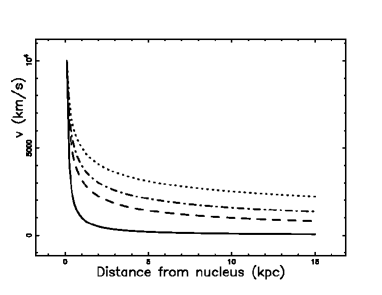
Figure 1: Classical velocity as a function of the distance from the nucleus when $x_{0}$ =100 pc and $v_{0}=10000\,$km/s: $\delta=0$ (full line), $\delta=1$ (dashes), $\delta=1.2$ (dot-dash-dot-dash) and $\delta=1.4$ (dotted).

3 Relativistic turbulent jets

The conservation of the momentum flux in special relativity, SR, in the presence of the velocity $v$ along one direction states that

$$(w(\frac{v}{c})^{2}\frac{1}{1-\frac{v^{2}}{c^{2}}}+p)A(x)=cost\quad,$$ (26)

where $A(x)$ is the considered area in the direction perpendicular to the motion, $c$ is the speed of light, and $w$ is the enthalpy per unit volume

$$w=c^{2}\rho+p\quad,$$ (27)

where $p$ is the pressure, see Gourgoulhon (2006) or formula A30 in De Young (2002). In accordance with the current models of classical turbulent jets, we insert $p=0$ and the conservation law for relativistic momentum flux is

$$(\rho v^{2}\frac{1}{1-\frac{v^{2}}{c^{2}}})A(x)=cost\quad.$$ (28)

Our physical units are pc for length and yr for time, and in these units, the speed of light is $c=0.306$  pc  yr^-1.

3.1 Constant density in SR

The conservation of the relativistic momentum flux when the density is constant can be written as the differential equation

$${\left({\frac{\rm d}{{\rm d}t}}x\left(t\right)\right)^{2}\pi\left(x\left(t\right)\right)^{2}\left(\tan\left(\frac{\alpha}{2}\right)\right)^{2}\left(1-{\frac{\left({\frac{\rm d}{{\rm d}t}}x\left(t\right)\right)^{2}}{{c}^{2}}}\right)^{-1}}$$

$$-{{v_{{0}}}^{2}\pi{{\it x_{0}}}^{2}\left(\tan\left(\frac{\alpha}{2}\right)\right)^{2}\left(1-{\frac{{v_{{0}}}^{2}}{{c}^{2}}}\right)^{-1}}=0\quad.$$ (29)

An analytical solution of the previous differential equations at the moment of writing does not exist but we can provide a power series solution of the form

$$x(t)=a_{0}+a_{1}t+a_{2}t^{2}+a_{3}t^{3}+\dots\quad,$$ (30)

see Tenenbaum and Pollard (1963); Ince (2012). The coefficients $a_{n}$ up to order 4 are

$$a_{0}= x_{{0}}$$

$$a_{1}= \beta_{{0}}c$$

$$a_{2}= \frac{1}{6}\,{\frac{3\,{c}^{2}{\beta_{{0}}}^{4}x_{{0}}-3\,{c}^{2}{\beta_{{0}}}^{2}x_{{0}}}{{x_{{0}}}^{2}}}$$

$$a_{3}= \frac{1}{6}\,{\frac{4\,{c}^{3}{\beta_{{0}}}^{7}-7\,{c}^{3}{\beta_{{0}}}^{5}+3\,{c}^{3}{\beta_{{0}}}^{3}}{{x_{{0}}}^{2}}}\quad,$$ (31)

where $\beta_{0}=\frac{v_{0}}{c}$.

In order to find a numerical solution of the above differential equation we isolate the velocity from eq.(29)

$$v(x;x_{0},\beta_{0},c)={\frac{x_{{0}}\beta_{{0}}{c}^{2}}{\sqrt{-{c}^{2}{x}^{2}{\beta_{{0}}}^{2}+{c}^{2}{\beta_{{0}}}^{2}{x_{{0}}}^{2}+{c}^{2}{x}^{2}}}}\,$$ (32)

and separate the variables

$$\int_{x_{0}}^{x}{\frac{\sqrt{-{c}^{2}{x}^{2}{\beta_{{0}}}^{2}+{c}^{2}{\beta_{{0}}}^{2}{x_{{0}}}^{2}+{c}^{2}{x}^{2}}}{x_{{0}}\beta_{{0}}{c}^{2}}}dx=\int_{0}^{t}dt\quad.$$ (33)

The integral on the left side of the previous equation has an analytical solution and the following non-linear equation is obtained

$$\frac{AN}{AD}=t\quad,$$ (34)

where

$$AN={\beta_{{0}}}^{2}{x_{{0}}}^{2}\ln\left(\sqrt{-{\beta_{{0}}}^{2}+1}x+\sqrt{-{x}^{2}{\beta_{{0}}}^{2}+{\beta_{{0}}}^{2}{x_{{0}}}^{2}+{x}^{2}}\right)$$

$$-{\beta_{{0}}}^{2}{x_{{0}}}^{2}\ln\left(\sqrt{-{\beta_{{0}}}^{2}+1}+1\right)$$

$$-{\beta_{{0}}}^{2}{x_{{0}}}^{2}\ln\left(x_{{0}}\right)+x\sqrt{-{x}^{2}{\beta_{{0}}}^{2}+{\beta_{{0}}}^{2}{x_{{0}}}^{2}+{x}^{2}}\sqrt{-{\beta_{{0}}}^{2}+1}$$

$$-{x_{{0}}}^{2}\sqrt{-{\beta_{{0}}}^{2}+1} ~{}\quad,$$ (35)

and

$$AD=2\,\sqrt{-{\beta_{{0}}}^{2}+1}x_{{0}}\beta_{{0}}\quad.$$ (36)

Figure 2 reports an example of the above numerical solution.

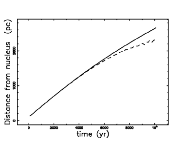
Figure 2: Non-linear solution as given by Eq. (34) (full line) and series solution as given by Eq. (30) (dashed line) when $x_{0}$ =100 pc and $\beta_{0}$ =0.999.

More details on the case of constant density can be found in Zaninetti (2009b).

3.2 A hyperbolic density profile in SR

The conservation of the relativistic momentum flux in the presence of an hyperbolic density profile as given by Eq. (16) is

$${{\it x_{0}}\,x\left(t\right)\left({\frac{\rm d}{{\rm d}t}}x\left(t\right)\right)^{2}\pi\,\left(\tan\left(\alpha/2\right)\right)^{2}\left(1-{\frac{\left({\frac{\rm d}{{\rm d}t}}x\left(t\right)\right)^{2}}{{c}^{2}}}\right)^{-1}}$$

$$-{{v_{{0}}}^{2}\pi\,{{\it x_{0}}}^{2}\left(\tan\left(\alpha/2\right)\right)^{2}\left(1-{\frac{{v_{{0}}}^{2}}{{c}^{2}}}\right)^{-1}}=0\quad.$$ (37)

The analytical solution of the previous differential equation is

$$x(t)=\frac{-\sqrt[3]{2}\sqrt[3]{x_{{0}}}\sqrt[3]{\left(3\,ct{\beta_{{0}}}^{3}-3\,ct\beta_{{0}}-2\,x_{{0}}\right)^{2}}+2\,{\beta_{{0}}}^{2}x_{{0}}}{2\,{\beta_{{0}}}^{2}-2}\quad.$$ (38)

The asymptotic approximation is

$$x(t)\sim-\frac{1}{2}\,{\frac{\sqrt[3]{2}\sqrt[3]{x_{{0}}}\sqrt[3]{9}\sqrt[3]{{\beta_{{0}}}^{2}{c}^{2}\left({\beta_{{0}}}^{2}-1\right)^{2}}}{\left({\beta_{{0}}}^{2}-1\right)\left({t}^{-1}\right)^{2/3}}}+{\frac{{\beta_{{0}}}^{2}x_{{0}}}{{\beta_{{0}}}^{2}-1}}$$

$$+\frac{2}{9}\,{\frac{\sqrt[3]{2}{x_{{0}}}^{4/3}\sqrt[3]{9}\sqrt[3]{{\beta_{{0}}}^{2}{c}^{2}\left({\beta_{{0}}}^{2}-1\right)^{2}}\sqrt[3]{{t}^{-1}}}{\beta_{{0}}c\left({\beta_{{0}}}^{2}-1\right)^{2}}}\quad.$$ (39)

The analytical solution when the velocity is expressed as $\beta=v/c$ is

$$\beta(t)=\frac{-\beta_{0}\,\left(3\,{\beta_{0}}^{3}ct-3\,\beta_{0}\,ct-2\,{\it x_{0}}\right)\sqrt[3]{{\it x_{0}}}\sqrt[3]{2}}{\left(\left(3\,{\beta_{0}}^{3}ct-3\,\beta_{0}\,ct-2\,{\it x_{0}}\right)^{2}\right)^{2/3}}\quad,$$ (40)

and the asymptotic approximation is

$$\beta(t)=\frac{-{\beta_{0}}^{2}c\left({\beta_{0}}^{2}-1\right)\sqrt[3]{{\it x_{0}}}\sqrt[3]{2}\sqrt[3]{9}\sqrt[3]{{t}^{-1}}}{3\,\left({\beta_{0}}^{2}{c}^{2}\left({\beta_{0}}^{2}-1\right)^{2}\right)^{2/3}}\quad.$$ (41)

3.3 Inverse power law profile of density in SR

The conservation of the relativistic momentum flux in the presence of a density profile of the inverse power law type as given by Eq. (23) is

$$\frac{-{x_{{0}}}^{\delta}{x}^{-\delta+2}{\beta_{{0}}}^{2}{\beta}^{2}+{\beta_{{0}}}^{2}{\beta}^{2}{x_{{0}}}^{2}+{x_{{0}}}^{\delta}{x}^{-\delta+2}{\beta}^{2}-{\beta_{{0}}}^{2}{x_{{0}}}^{2}}{\left({\beta}^{2}-1\right)\left({\beta_{{0}}}^{2}-1\right)}=0\quad.$$ (42)

This differential equation does not have an analytical solution and the expression for $\beta$ as a function of the distance is

$$\beta(x)=\frac{x_{{0}}\beta_{{0}}}{\sqrt{-{\beta_{{0}}}^{2}{x}^{2}\left({\frac{x_{{0}}}{x}}\right)^{\delta}+{\beta_{{0}}}^{2}{x_{{0}}}^{2}+{x}^{2}\left({\frac{x_{{0}}}{x}}\right)^{\delta}}}\quad.$$ (43)

The behavior of $\beta$ as a function of the distance for different values of $\delta$ can be seen in Figure 3.

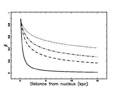
Figure 3: Relativistic variable $\beta$ as a function of the distance from the nucleus when $x_{0}$ =100 pc and $\beta_{0}$ =0.9: $\delta=0$ (full line), $\delta=1$ (dashes), $\delta=1.2$ (dot-dash-dot-dash) and $\delta=1.4$ (dotted).

The transit time can be derived from Eq. (39)

$$t_{tr}=\frac{2\,{{\it x_{0}}}^{2}-2\,\sqrt{{\it x_{0}}\,\left({\beta_{0}}^{2}{\it x_{0}}-{\beta_{0}}^{2}{\it x_{max}}+{\it x_{max}}\right)^{3}}}{3\,\beta_{0}\,c\left({\beta_{0}}^{2}-1\right){\it x_{0}}}\quad.$$ (44)

As an example, inserting $x_{0}$=100 pc, $x_{max}=15\,10^{3}\,$pc, and $\beta_{0}=0.9$, we have $t_{tr}=2\,10^{5}\,$yr.

4 Classical curved trajectories

In the presence of a 3D trajectory, ${\bf{r(t)}}$, the acceleration is given by

$${\bf{a}}=\frac{dv}{dt}{\bf{T}}+\frac{v^{2}}{\rho}{\bf{N}}\quad,$$ (45)

where $v=|\frac{d{\bf{r(t)}}}{dt}|=|\frac{ds}{dt}$ is the magnitude of the velocity, $s$ is the arc-length of the trajectory, ${\bf{T}}$ and ${\bf{N}}$ are the tangential and normal versors to the trajectory, and $R$ is the radius of curvature given by

$$R=\left((\frac{d^{2}x}{ds^{2}})^{2}+(\frac{d^{2}y}{ds^{2}})^{2}+(\frac{d^{2}z}{ds^{2}})^{2}\right)^{-1/2}\quad,$$ (46)

see exercise 5.30 in Spiegel (1971). A second definition of the radius of curvature when we have a 2D curve parametrized as $y(x)$ is

$$R=\frac{\left(1+\left(\frac{dy}{dx}\right)^{2}\right)^{\frac{3}{2}}}{\frac{d^{2}y}{dx^{2}}}\quad,$$ (47)

see Eq. (12.5) in Granville (1911). In the presence of a trajectory given by a discrete set of points, the circle of curvature which has radius $R_{c}$, and coordinates of its centre $(x_{c},y_{c})$, can be drawn when three points are given, see Appendix A. According to theorem 14.1.1 in Granville (1911), the radius of the circle of curvature and the radius of curvature are equal.

4.1 The astronomical data

As an application, we analyse the first part of the right side of NGC 1265 where the distances were evaluated adopting $H_{0}=50\mathrm{km\,s^{-1}\,Mpc^{-1}}$ for the Hubble constant and $z=0.0183$ for the redshift see Xu et al. (1999). At the moment of writing, there is a more precise evaluation of the Hubble constant, which is $H_{0}=(69.6\pm 0.7)\mathrm{km\,s^{-1}\,Mpc^{-1}}$, see Bennett et al. (2014), which, coupled with $c=299792.458\mathrm{\frac{km}{s}}$ for the velocity of light, see Mohr et al. (2012), means

$$1^{\prime\prime}=382.15pc\quad.$$ (48)

The trajectory of NGC 1265 was derived as follows

1. The data were digitized in $~{}^{\prime\prime}$ from Figure 3 in Owen et al. (1978) using WebPlotDigitizer, a Web based tool to extract data from plots.

2. The conversion from $~{}^{\prime\prime}$ to pc was done using Eq. (48).

Figure 4 shows the digitalized 2D trajectory and 8 circles of curvature computed according to Eqs (A.1, A.2,A.3).

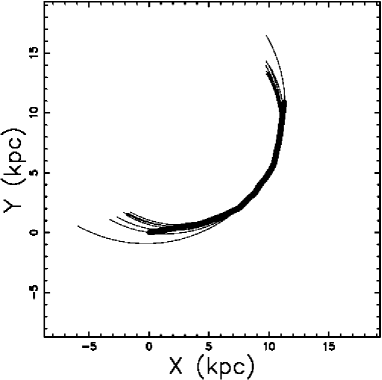
Figure 4: The right side of NGC 1265 , the line with a large width, represents the real data as extracted by the author from Figure 3 in Owen, Burns, $\&$ Rudnick (1978) and 8 circles of curvature.

The average radius of the circle of curvature, $\overline{R_{c}}$, for the first 20 kpc of the right side of NGC 1265 is

$$\overline{R_{c}}=(9.22\pm 1.03)kpc\quad.$$ (49)

4.2 Curved trajectory with constant density

A ballistic trajectory is determined on Earth by gravity and aerodynamic drag. Here we assume a non-ballistic trajectory for the radio-galaxy as being due to the composition of the jet’s motion along the $x$-axis with a motion at constant velocity, $v_{g}$, of the parent galaxy along the $y$-axis. The peculiar velocity for a galaxy with redshift $z$ can be evaluated using formula (3) in Freeland et al. (2008). Other authors replace the velocity of the parent galaxy with the velocity of external winds, see Hardee and Hughes (2003); Perkins et al. (2004).

When the galaxy’s velocity is expressed in km s^-1, the multiplicative factor $1.02\times 10^{-6}$ should be applied in order to have the galaxy’s velocity expressed in $\mathrm{pc\,yr^{-1}}$. The two equations of motion are

$$x(t)=\sqrt{2\,tv_{{0}}x_{{0}}+{x_{{0}}}^{2}}$$ (50a)

$$y(t)=y_{0}+v_{g}t\quad,$$ (50b)

where $y_{0}$ is the $y$-position at $t=0$. In order to evaluate the radius of curvature in the case of constant density, we extract $t$ from Eq. (50a) and we insert it into Eq. (50b)

$$y(x)=\frac{1}{2}\,{\frac{v_{{g}}\left({x}^{2}-{x_{{0}}}^{2}\right)}{v_{{0}}x_{{0}}}}+y_{{0}}\quad.$$ (51)

The previous formula allows visualizing the trajectory which represents the best fit for the right side of NGC 1265 in the case of constant density, see Figure 5.

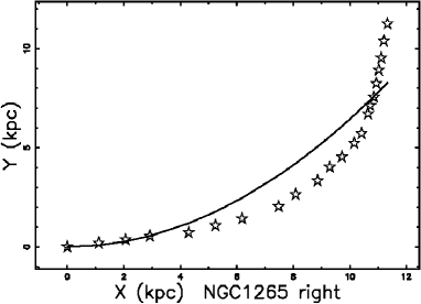
Figure 5: Real trajectory of NGC 1265 (big stars) and theoretical curved trajectory (full line) in the case of constant density. The parameters are $x_{0}$=100 pc, $y_{0}$=0 pc, $v_{0}=$9620  km/s and $v_{g}=$ 124 km/s.

The parameters $v_{0}$ and $v_{g}$ are found by minimizing the value of $\chi^{2}$ defined as

$$\chi^{2}=\sum_{i=1}^{n}(y_{i}-y_{i,th})^{2}\quad,$$ (52)

where $y_{i}$ is the $y$-value of the $i$th point in the digitized trajectory and $y_{i,th}$ is the theoretical point obtained by inserting the $x$ value of the $i$th point in Eq. (51).

The radius of curvature in the case of constant density as given by Eq. (46) is

$$R={\frac{\left({x}^{2}{v_{{g}}}^{2}+{v_{{0}}}^{2}{x_{{0}}}^{2}\right)^{3/2}}{{v_{{0}}}^{2}{x_{{0}}}^{2}v_{{g}}}}\quad,$$ (53)

as a consequence the centripetal acceleration is

$$\frac{v^{2}}{R}{\bf{N}}={\frac{\left(2\,tv_{{0}}x_{{0}}+{x_{{0}}}^{2}+\left(tv_{{g}}+y_{{0}}\right)^{2}\right){v_{{0}}}^{2}{x_{{0}}}^{2}v_{{g}}}{\left({v_{{0}}}^{2}{x_{{0}}}^{2}+{v_{{g}}}^{2}\left(2\,tv_{{0}}x_{{0}}+{x_{{0}}}^{2}\right)\right)^{3/2}}}{\bf{N}}\quad.$$ (54)

4.3 Curved trajectory with hyperbolic density

In the case of an hyperbolic density profile we can isolate the time in Eq. (18) and insert it into Eq. (50b). The resulting trajectory, which is independent of the time, is

$$y(x)=-\frac{2}{3}\,{\frac{v_{{g}}\left({x_{{0}}}^{3/2}-{x}^{3/2}\right)}{\sqrt{x_{{0}}}v_{{0}}}}+y_{{0}}\quad.$$ (55)

The trajectory which represents the best fit for the right side of NGC 1265 in the case of an hyperbolic density profile is shown in Figure 6.

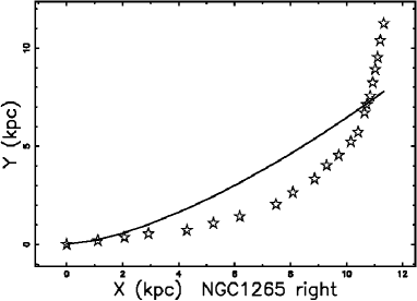
Figure 6: Real trajectory of NGC 1265 (big stars) and theoretical curved trajectory (full line) in the case of an hyperbolic profile of density. The parameters are $x_{0}$=100  pc, $y_{0}$=0   pc, $v_{0}=$3660 km/s and $v_{g}=$54.74 km/s.

The radius of curvature in the case of an hyperbolic profile of density as given by Eq. (46) is

$$R=2\,{\frac{\left(x{v_{{g}}}^{2}+{v_{{0}}}^{2}x_{{0}}\right)^{3/2}\sqrt{x}}{{v_{{0}}}^{2}x_{{0}}v_{{g}}}}\quad,$$ (56)

and the centripetal acceleration is

$$\frac{v^{2}}{R}{\bf{N}} =~{}$$

$$\frac{\left(A+\left(12\,tv_{{0}}{x_{{0}}}^{2}+8\,{x_{{0}}}^{3}\right)^{4/3}+16\,{x_{{0}}}^{2}{y_{{0}}}^{2}\right){v_{{0}}}^{2}x_{{0}}\sqrt{4}v_{{g}}}{32\,{x_{{0}}}^{2}\left({v_{{0}}}^{2}x_{{0}}+1/4\,{\frac{{v_{{g}}}^{2}\left(12\,tv_{{0}}{x_{{0}}}^{2}+8\,{x_{{0}}}^{3}\right)^{2/3}}{x_{{0}}}}\right)^{3/2}\sqrt{{\frac{\left(12\,tv_{{0}}{x_{{0}}}^{2}+8\,{x_{{0}}}^{3}\right)^{2/3}}{x_{{0}}}}}}{\bf{N}} ~{}\quad,$$ (57)

where

$$A=16\,{t}^{2}{v_{{g}}}^{2}{x_{{0}}}^{2}+32\,tv_{{g}}{x_{{0}}}^{2}y_{{0}}\quad.$$ (58)

5 The helicoidal trajectory

The circular helix is

$$x=a\,cos(t)$$ (59a)

$$y=a\,sin(t)$$ (59b)

$$z=b\,t\quad$$ (59c)

where $a$ is the radius and the pitch is $2\,\pi\,b$, see Lipschutz (1969). The radius of curvature of the circular helix is

$$R=\frac{a^{2}+b^{2}}{a}\quad.$$ (60)

The arc-length of the helix, $s$, as a function of time is

$$s=\sqrt{a^{2}+b^{2}}\,t\quad.$$ (61)

The helicoidal jet in the case of constant density is

$$x=\sqrt{2\,tv_{{0}}x_{{0}}+{x_{{0}}}^{2}}$$ (62a)

$$y=at\cos\left(\Omega_{{p}}t\right)$$ (62b)

$$z=at\sin\left(\Omega_{{p}}t\right)\quad,$$ (62c)

where the $x-t$ relationship is given by Eq. (11), $\Omega_{{p}}$ is the angular velocity, and the radius of the helix grows linearly with time according to a linear relationship given by the parameter $a$. The pitch of the helicoidal jet is

$$\sqrt{4\,{\frac{\pi\,v_{{0}}x_{{0}}}{\Omega_{{p}}}}+{x_{{0}}}^{2}}\quad.$$ (63)

The radius of curvature of the helicoidal jet is

$$R=\frac{NH}{DH}\quad,$$ (64)

where

$$NH=\left(2\,{a}^{2}{t}^{3}{\Omega_{{p}}}^{2}v_{{0}}+{a}^{2}{t}^{2}{\Omega_{{p}}}^{2}x_{{0}}+2\,{a}^{2}tv_{{0}}+{a}^{2}x_{{0}}+{v_{{0}}}^{2}x_{{0}}\right)^{3/2}\quad,$$ (65)

$$DH=~{}$$

$$a\Big{(}8\,{a}^{2}{t}^{7}{\Omega_{{p}}}^{6}{v_{{0}}}^{3}+12\,{a}^{2}{t}^{6}{\Omega_{{p}}}^{6}{v_{{0}}}^{2}x_{{0}}+6\,{a}^{2}{t}^{5}{\Omega_{{p}}}^{6}v_{{0}}{x_{{0}}}^{2}+{a}^{2}{t}^{4}{\Omega_{{p}}}^{6}{x_{{0}}}^{3}$$

$$+32\,{a}^{2}{t}^{5}{\Omega_{{p}}}^{4}{v_{{0}}}^{3}+48\,{a}^{2}{t}^{4}{\Omega_{{p}}}^{4}{v_{{0}}}^{2}x_{{0}}+4\,{t}^{4}{\Omega_{{p}}}^{4}{v_{{0}}}^{4}x_{{0}}+24\,{a}^{2}{t}^{3}{\Omega_{{p}}}^{4}v_{{0}}{x_{{0}}}^{2}$$

$$+4\,{t}^{3}{\Omega_{{p}}}^{4}{v_{{0}}}^{3}{x_{{0}}}^{2}+4\,{a}^{2}{t}^{2}{\Omega_{{p}}}^{4}{x_{{0}}}^{3}+{t}^{2}{\Omega_{{p}}}^{4}{v_{{0}}}^{2}{x_{{0}}}^{3}+32\,{a}^{2}{t}^{3}{\Omega_{{p}}}^{2}{v_{{0}}}^{3}$$

$$+48\,{a}^{2}{t}^{2}{\Omega_{{p}}}^{2}{v_{{0}}}^{2}x_{{0}}+21\,{t}^{2}{\Omega_{{p}}}^{2}{v_{{0}}}^{4}x_{{0}}+24\,{a}^{2}t{\Omega_{{p}}}^{2}v_{{0}}{x_{{0}}}^{2}$$

$$+18\,t{\Omega_{{p}}}^{2}{v_{{0}}}^{3}{x_{{0}}}^{2}+4\,{a}^{2}{\Omega_{{p}}}^{2}{x_{{0}}}^{3}+4\,{\Omega_{{p}}}^{2}{v_{{0}}}^{2}{x_{{0}}}^{3}+{v_{{0}}}^{4}x_{{0}}\Big{)}^{1/2}\,.$$ (66)

Figure 7 shows the radius of curvature of the helicoidal jet in kpc as a function of time in units of $10^{7}$ years.

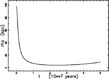
Figure 7: The radius of curvature of the helicoidal jet versus time when the parameters are $x_{0}$=100 pc, $y_{0}$=0 pc, and $v_{0}=$9620  km/s.

The bent helicoidal jet in the case of constant density is

$$x=\sqrt{2\,tv_{{0}}x_{{0}}+{x_{{0}}}^{2}}$$ (67a)

$$y=at\cos\left(\Omega_{{p}}t\right)$$ (67b)

$$z=at\sin\left(\Omega_{{p}}t\right)+z_{0}+v_{g}t\quad.$$ (67c)

A 3D display of the bent helicoidal jet is shown in Figure 8, where the choice of the Euler angles, which define the observer, corresponds to the astronomical observations.

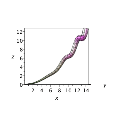
Figure 8: Continuous 3D surface of NGC 1265 : the three Eulerian angles characterizing the point of view are $\Phi$= 0 ^∘, $\Theta$= 90 ^∘, and $\Psi$= 0 ^∘. The physical parameters are $x_{0}$=100 pc, $y_{0}$=0 pc, $v_{0}=$9620 km/s, $v_{g}=$124 km/s, $\Omega_{{p}}=6\,10^{-8}\,\pi\,\frac{rad}{years}$ and $alpha=5^{\circ}$. The axes are expressed in kpc units.

Another choice of the Euler angles produces a different projected surface, see Figure 9.

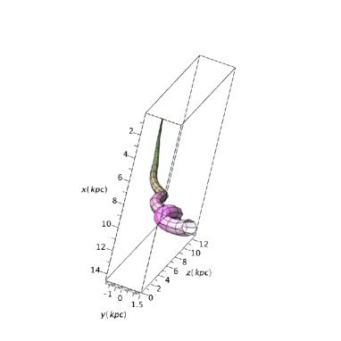
Figure 9: Continuous 3D surface of NGC 1265 : the three Eulerian angles characterizing the point of view are $\Phi$= 70 ^∘, $\Theta$= 20 ^∘, and $\Psi$= 10 ^∘. The physical parameters are the same as in Figure 8 and the axes are expressed in kpc units.

The radius of curvature of the bent helicoidal jet has a complicated expression and we only present its numerical behavior, see Figure 10.

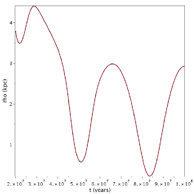
Figure 10: The radius of curvature of the bent helicoidal jet versus time. The physical parameters are the same as Figure 8.

The arc-length of the bent helicoidal jet is

$$s=\int_{0}^{t}\sqrt{\frac{NS}{DS}\,dt}\quad,$$ (68)

where

$$NS=2\,{a}^{2}{\Omega_{{p}}}^{2}{t}^{3}v_{{0}}+{a}^{2}{\Omega_{{p}}}^{2}{t}^{2}x_{{0}}+4\,\cos\left(\Omega_{{p}}t\right)a\Omega_{{p}}{t}^{2}v_{{0}}v_{{g}}+2\,{a}^{2}tv_{{0}}$$

$$+2\,\cos\left(\Omega_{{p}}t\right)a\Omega_{{p}}tv_{{g}}x_{{0}}+{a}^{2}x_{{0}}+4\,\sin\left(\Omega_{{p}}t\right)atv_{{0}}v_{{g}}$$

$$+2\,\sin\left(\Omega_{{p}}t\right)av_{{g}}x_{{0}}+2\,tv_{{0}}{v_{{g}}}^{2}+{v_{{0}}}^{2}x_{{0}}+{v_{{g}}}^{2}x_{{0}}\quad,$$ (69)

and

$$DS=2\,tv_{{0}}+x_{{0}}\quad.$$ (70)

The previous integral does not have an analytical expression and the numerical integration between 0 and $10^{8}$ years, the other parameters as in Figure 10, gives $s=22.2\,$pc.

6 The theory of images

In the case of an optically thin layer, the emissivity is proportional to the number density, $C$,

$$j_{\nu}\zeta=KC(s)\quad,$$ (71)

where $j_{\nu}$ is the emission coefficient and $K$ is a constant. This can be the case for synchrotron radiation in the presence of an isotropic distribution of electrons with a power law distribution in energy, $N(E)$,

$$N(E)dE=K_{s}E^{-\gamma}\quad,$$ (72)

where $K_{s}$ and $\gamma$ are constants, see Zaninetti (2010) for more details. In the case of constant number density

$$j_{\nu}\zeta=K\,C\,s\quad,$$ (73)

where $s$ is the length of the relevant line of sight, this formula is extremely simple and allows building the image in the appropriate geometrical environment. Two analytical results outline the theoretical framework that should be verified by the simulation. The first one analyses the behavior of the intensity or brightness along a jet when the distance from the origin, $x$, is fixed. We assume that the number density $C$ is constant in a cross section of radius $a$ and then falls to 0, see Figure 11.

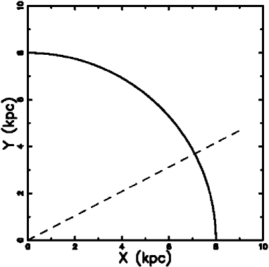
Figure 11: The source is represented through a circular section perpendicular to the jet axis. The observer is situated along the $y$-direction, one line of sight is indicated and the angle $\beta$ is clearly indicated.

The length of sight, when the observer is situated at the infinity of the $y$-axis, is the locus parallel to the $y$-axis which crosses the position $x$ in a Cartesian $x-y$ plane and terminates at the external circle of radius $a$. The locus length is

$$l_{ab}=2\times(\sqrt{a^{2}-x^{2}})\quad;0\leq x<a\quad.$$ (74)

When the number density $C$ is constant on a cylinder of radius $a$, the intensity or brightness of radiation is

$$I_{0a}=C\times 2\times(\sqrt{a^{2}-x^{2}})\quad;0\leq x<a\quad,$$ (75)

or

$$I_{0a}=C\times 2\times a\times\sin(\beta)\quad;-\frac{\pi}{2}\leq\beta\leq\frac{\pi}{2}\quad,$$ (76)

which can be called the ‘trigonometrical law’ for the intensity or brightness. The second analytical result can be derived when the curved shape of a jet of finite cross section is parametrized by a toroidal helix. The toroidal helix has the following parametric equations:

$$x=\cos(\alpha)\cdot(R+r\cdot\cos(\theta))$$

$$y=\sin(\alpha)\cdot(R+r\cdot\cos(\theta))$$ (77)

$$z=r\cdot\sin(\theta)+\alpha\frac{n\,r}{2\pi}\quad,$$

where $\theta\in[0,2\pi)$, $\alpha\in[0,2\pi)$, $n\,r$ is the distance along the $z$-axis after an angle $\alpha=2\pi$, and $n$ is an integer. We now analyse the case in which

$$\alpha\ll\frac{2\pi}{n}\quad,$$ (79)

where the right-hand side is the value of the angle after which the toroidal helix has advanced by $r$ along the $z$-direction. Figure 12 shows a section in the middle of the toroidal helix $z=0$, from which is possible to see that the dotted line presents the longest line of sight, $l_{max}$, which starts from $x=R$ when the observer is at the infinity of the $y$-axis.

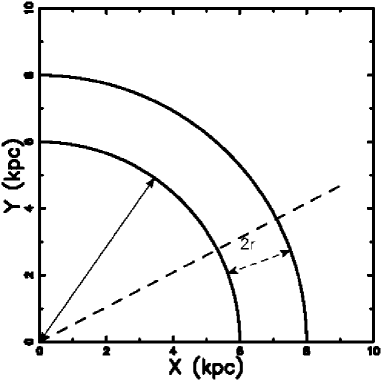
Figure 12: The section of one-fourth of a toroidal helix is represented through a circle of radius $R-r$ and a bigger circle of radius $R+r$. The observer is situated along the $y$-direction at infinity and the line of sight of maximum length is indicated.

The shortest line of sight is $2r$. The maximum enhancement in the presence of a constant number density, $e$, is

$$e=\frac{l_{max}}{2r}.$$ (80)

A simple geometrical demonstration gives

$$e=\frac{1}{2}\,{\frac{\sqrt{2\,R+r}}{\sqrt{r}}}\quad.$$ (81)

The relationship between the radius of curvature, $R$, and the radius of the toroidal helix, $r$, which produces an enhancement $e$ in the intensity or brightness is

$$\frac{R}{r}=2\,{e}^{2}-\frac{1}{2}\quad.$$ (82)

We now outline how it is possible to build a radio-image. The number density is stored on a 3D grid ${\mathcal{M}(i,j,k)}$ where $i,j$ and $k$ are indices varying from 1 to $pixels$. The orientation of the object is characterized by the Euler angles $(\Phi,\Theta,\Psi)$ and therefore by a $3\times 3$ rotation matrix, $E$, see Goldstein et al. (2002). The grid ${\mathcal{M}(i,j,k)}$ is then rotated according to the chosen Euler angles. The intensity map is obtained by summing the points of the rotated images along a particular direction, and the intensity is

$${\it I}\/(i,j)=\sum_{k}\triangle\,s\times{\mathcal{M}}(i,j,k)$$ (83)

$$\quad\mbox{optically thin layer}\quad linear~{}case\quad,$$

where $\triangle$s is the spatial interval between the various values of intensity and the sum is performed over the interval of existence of the index $k$. In this grid the little squares that are characterized by the position of the indexes $i,j$ correspond to a different line of sight.

The effect of the insertion of a threshold intensity, $I_{tr}$, given by the observational techniques, is now analysed. The threshold intensity can be parametrized to $I_{max}$, the maximum value of intensity characterizing the map,

$$I_{tr}=\frac{I_{max}}{factor}\quad,$$ (84)

where the parameter factor is greater than one.

A map for the emissivity of a jet can be built by employing the following algorithm:

• A great number of points, for example, one million, is inserted into a bent helicoidal jet with given characteristic parameters.

• This set of points is rotated according to the three Euler angles which identify the observer’s point of view.

• The 2D matrix which represents the intensity of the non-thermal emission is built according to procedure (6).

Figure 13 shows the projected points.

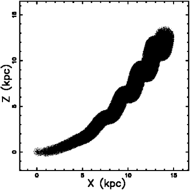
Figure 13: Continuous 3D trajectory of NGC 1265 : the three Eulerian angles characterizing the point of view are $\Phi$= 0 ^∘, $\Theta$= 90 ^∘, and $\Psi$= 0 ^∘. The physical parameters are the same as Figure 8.

The two analytical results, the enhancement of the intensity in the central line and the knot structure due to the curvature along the line of sight, are clearly visible in Figure 14, which shows the intensity of a non-thermal map of NGC 1265 .

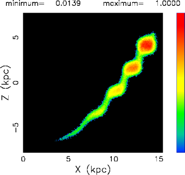
Figure 14: Theoretical 2D map of the surface brightness of the emission of NGC 1265 with basic parameters as in Figure 13. The integration is performed on a cubic grid of $1000^{3}$ pixels and factor = 4.

A first comparison of the previous figure can be done with Figure 1 in Aloy et al. (2003) where a 3D relativistic hydrodynamic simulation for the precessing beam was carried out. A second comparison can be done with the pseudo-synchrotron intensities visible in the figures of Hardee and Hughes (2003); Hardee et al. (2005) where the knots in the radio-jets were simulated in the framework of helical relativistic instabilities. A third comparison can be done with Figure 3 in Laing and Bridle (2014) where the observed and model total-intensity images are reported for 15 radio-galaxies without bending effects.

7 Conclusions

Classical turbulence: Turbulent jets are usually modeled by a temporal evolution with density equal to that of the surrounding medium. Here, in order to cover the astrophysical applications, we considered an hyperbolic profile of density, see the solution (18) and an asymptotic solution (19). The case of a density which follows an inverse power law is limited to the derivation of the velocity, see Eq. (25). This inverse power law case allows matching a wide variety of astrophysical situations, as an example, when $\delta=2$, the velocity does not decreases with distance.

This is obvious from the conservation equation, $\rho vA$ = constant. If $A$ goes as $r^{2}$ and $\rho$ goes with the inverse of the square of distance in a conical jet, $v$ is constant.

Relativistic turbulence: The conservation of the relativistic momentum flux for turbulent jets is here analysed in three cases. The first case is that with a surrounding medium having constant density, where the analytical result is limited to a series expansion for the solution, see Eq. (30). The second case is that of an hyperbolic density decrease for the surrounding medium, for which we derived an analytical solution see Eq. (38) and an asymptotic solution, see Eq. (39). The third case is that where the surrounding density decreases with a power law behavior: the analytical result is limited to the velocity–distance relationship, see Eq. (43).

The curvature of the jet: The composition of the velocity is discussed in the light of the radius of curvature and the standard mathematical definition is given, see Eq. (47). The astronomical counterpart is the radius of the circle of curvature which is shown in Figure 4 for NGC 1265 . Two analytical solutions are given for the curved trajectory, see Eqs (50a) and (50b), in the case of constant density and Eq. (55) for an hyperbolic decrease in density. A careful analysis of Figures 5 and 6 does not show an accurate coincidence between the predictions of the model and the digitized trajectory. In this case, its $\chi^{2}$ can be lowered by introducing other effects such as photon losses due to synchrotron radiation or another density profile.

Helicoidal bent jet: The precession is here modeled by an helicoidal jet, see Eq. 62, which has a pitch and radius of curvature given by Eqs (63) and (64). The composition with the velocity of the host galaxy allows modelling the a helicoidal jet in which the radius of curvature can be visualized only numerically, see Figure 10. The arc-length has a complicated expression, which is given by Eq. (68).

Theoretical radio maps: The radio image of an extragalactic radio source is built adopting: (i) a uniform number density of synchrotron emitters over the entire jet, (ii) the thin layer approximation. The two theoretical effects of central brightening, see Eq. (76), and intensity brightening due to the curvature of the emitting region, see Eq. (81), are both visible in the simulation of NGC 1265 , see Figure 14.

New analytical results can be obtained expressing the helicoidal trajectory in cylindrical coordinates or analysing the ‘valley on the top’ effect which is due to the velocity profile in the direction perpendicular to the motion, see Zaninetti (2009a). The previously cited papers solve some of the problems connected with the radio-jets but leave other problems open, and Table 1 reports their status.

Table 1: Synoptic table of the assumptions of two papers and here

$$\begin{array}[]{lccc}\hline\cr\hline\cr\vskip 3.0pt plus 1.0pt minus 1.0pt\cr Problem&Laing\&Bridle\,2002&Hardee\,et\,al.2005&this~{}paper\\ \vskip 3.0pt plus 1.0pt minus 1.0pt\cr\hline\cr\vskip 3.0pt plus 1.0pt minus 1.0pt\cr distance~{}along~{}the~{}jet&numerical&not&analytical\\ velocity~{}along~{}the~{}jet&numerical&not&analytical\\ knots&not&instabilities&image~{}theory\\ \vskip 3.0pt plus 1.0pt minus 1.0pt\cr\vskip 3.0pt plus 1.0pt minus 1.0pt\cr\hline\cr\end{array}$$

Appendix A The circle of curvature

Once three points are selected on a curve, $(x_{1},y_{1}),(x_{2},y_{2}),(x_{3},y_{3})$, the circle of curvature has radius

$$R_{c}=\frac{NR}{DR}\quad,$$ (A.1)

where

$$NR=\Bigg{\{}\left({x_{{2}}}^{2}-2\,x_{{2}}x_{{3}}+{x_{{3}}}^{2}+{y_{{2}}}^{2}-2\,y_{{2}}y_{{3}}+{y_{{3}}}^{2}\right)\times$$

$$\left({x_{{1}}}^{2}-2\,x_{{1}}x_{{3}}+{x_{{3}}}^{2}+{y_{{1}}}^{2}-2y_{{1}}y_{{3}}+{y_{{3}}}^{2}\right)\times$$

$$\left({x_{{1}}}^{2}-2\,x_{{1}}x_{{2}}+{x_{{2}}}^{2}+{y_{{1}}}^{2}-2\,y_{{1}}y_{{2}}+{y_{{2}}}^{2}\right)\Bigg{\}}^{(1/2)} \quad,$$

$$DR=2\,x_{{1}}y_{{2}}-2\,x_{{1}}y_{{3}}-2\,x_{{2}}y_{{1}}+2\,x_{{2}}y_{{3}}+2\,x_{{3}}y_{{1}}-2\,x_{{3}}y_{{2}}\quad.$$

The two coordinates of the centre of the circle, ($x_{c},y_{c}$), are

$$x_{c}=\frac{NXC}{DXC}\quad,$$ (A.2)

where

$$NXC={x_{{1}}}^{2}y_{{2}}-{x_{{1}}}^{2}y_{{3}}-{x_{{2}}}^{2}y_{{1}}+{x_{{2}}}^{2}y_{{3}}+{x_{{3}}}^{2}y_{{1}}-{x_{{3}}}^{2}y_{{2}}+{y_{{1}}}^{2}y_{{2}}$$

$$-{y_{{1}}}^{2}y_{{3}}-y_{{1}}{y_{{2}}}^{2}+y_{{1}}{y_{{3}}}^{2}+{y_{{2}}}^{2}y_{{3}}-y_{{2}}{y_{{3}}}^{2}\quad,$$

$$DXC=2\,x_{{1}}y_{{2}}-2\,x_{{1}}y_{{3}}-2\,x_{{2}}y_{{1}}+2\,x_{{2}}y_{{3}}+2\,x_{{3}}y_{{1}}-2\,x_{{3}}y_{{2}}\quad,$$

and

$$y_{c}=\frac{NYC}{DYC}\quad,$$ (A.3)

where

$$NYC=-{x_{{1}}}^{2}x_{{2}}+{x_{{1}}}^{2}x_{{3}}+x_{{1}}{x_{{2}}}^{2}-x_{{1}}{x_{{3}}}^{2}+x_{{1}}{y_{{2}}}^{2}-x_{{1}}{y_{{3}}}^{2}$$

$$-{x_{{2}}}^{2}x_{{3}}+x_{{2}}{x_{{3}}}^{2}-x_{{2}}{y_{{1}}}^{2}+x_{{2}}{y_{{3}}}^{2}+x_{{3}}{y_{{1}}}^{2}-x_{{3}}{y_{{2}}}^{2}\quad,$$

$$DYC=2\,x_{{1}}y_{{2}}-2\,x_{{1}}y_{{3}}-2\,x_{{2}}y_{{1}}+2\,x_{{2}}y_{{3}}+2\,x_{{3}}y_{{1}}-2\,x_{{3}}y_{{2}}\quad.$$

References

- Aloy et al. (2003) Aloy, M.-Á., Martí, J.-M., Gómez, J.-L., Agudo, I., Müller, E., and Ibáñez, J.-M. (2003), “Three-dimensional Simulations of Relativistic Precessing Jets Probing the Structure of Superluminal Sources,” ApJ , 585, L109–L112.
- Bennett et al. (2014) Bennett, C. L., Larson, D., Weiland, J. L., and Hinshaw, G. (2014), “The 1% Concordance Hubble Constant,” ApJ , 794, 135.
- Bicknell (1984) Bicknell, G. V. (1984), “A model for the surface brightness of a turbulent low Mach number jet. I - Theoretical development and application to 3C 31,” ApJ , 286, 68–87.
- Bicknell and Melrose (1982) Bicknell, G. V. and Melrose, D. B. (1982), “In situ acceleration in extragalactic radio jets,” ApJ , 262, 511–528.
- Bowman et al. (1996) Bowman, M., Leahy, J. P., and Komissarov, S. S. (1996), “The deceleration of relativistic jets by entrainment,” MNRAS , 279, 899.
- Burns and Owen (1980) Burns, J. O. and Owen, F. N. (1980), “Dual curved jets in the tailed radio galaxy 1638 + 538 /4C53.37/,” AJ , 85, 204–214.
- Burns et al. (1979) Burns, J. O., Owen, F. N., and Rudnick, L. (1979), “The wide-angle tailed radio galaxy 1159 + 583 - Observations and models,” AJ , 84, 1683–1693.
- Curtis (1918) Curtis, H. D. (1918), “Descriptions of 762 Nebulae and Clusters Photographed with the Crossley Reflector,” Publications of Lick Observatory, 13, 9–42.
- De Young (2002) De Young, D. S. (2002), The physics of extragalactic radio sources, Chicago: University of Chicago Press.
- Freeland et al. (2008) Freeland, E., Cardoso, R. F., and Wilcots, E. (2008), “Bent-Double Radio Sources as Probes of Intergalactic Gas,” ApJ , 685, 858–862.
- Goldstein et al. (2002) Goldstein, H., Poole, C., and Safko, J. (2002), Classical mechanics, San Francisco: Addison-Wesley.
- Gourgoulhon (2006) Gourgoulhon, E. (2006), “An introduction to relativistic hydrodynamics,” EAS PUBL.SER., 21, 43.
- Granville (1911) Granville, W. A. (1911), Elements of the differential and integral calculus. Revised edition., New York: Ginn and Co.
- Hardcastle and Sakelliou (2004) Hardcastle, M. J. and Sakelliou, I. (2004), “Jet termination in wide-angle tail radio sources,” MNRAS , 349, 560–575.
- Hardee and Hughes (2003) Hardee, P. E. and Hughes, P. A. (2003), “The Effect of External Winds on Relativistic Jets,” ApJ , 583, 116–123.
- Hardee et al. (2005) Hardee, P. E., Walker, R. C., and Gómez, J. L. (2005), “Modeling the 3C 120 Radio Jet from 1 to 30 Milliarcseconds,” ApJ , 620, 646–664.
- Ince (2012) Ince, E. L. (2012), Ordinary differential equations, New York: Courier Dover Publications.
- Jaffe and Perola (1973) Jaffe, W. J. and Perola, G. C. (1973), “Dynamical Models of Tailed Radio Sources in Clusters of Galaxies,” A&A , 26, 423–+.
- Laing and Bridle (2002a) Laing, R. A. and Bridle, A. H. (2002a), “Dynamical models for jet deceleration in the radio galaxy 3C 31,” MNRAS , 336, 1161–1180.
- Laing and Bridle (2002b) — (2002b), “Relativistic models and the jet velocity field in the radio galaxy 3C 31,” MNRAS , 336, 328–352.
- Laing and Bridle (2004) — (2004), “Adiabatic relativistic models for the jets in the radio galaxy 3C 31,” MNRAS , 348, 1459–1472.
- Laing and Bridle (2014) — (2014), “Systematic properties of decelerating relativistic jets in low-luminosity radio galaxies,” MNRAS , 437, 3405–3441.
- Laing et al. (2006) Laing, R. A., Canvin, J. R., Bridle, A. H., and Hardcastle, M. J. (2006), “A relativistic model of the radio jets in 3C296,” MNRAS , 372, 510–536.
- Landau (1987) Landau, L. (1987), Fluid Mechanics 2nd edition, New York: Pergamon Press.
- Lipschutz (1969) Lipschutz, M. (1969), Schaum’s Outline of Differential Geometry, New York: McGraw-Hill.
- Melia and Konigl (1989) Melia, F. and Konigl, A. (1989), “The radiative deceleration of ultrarelativistic jets in active galactic nuclei,” ApJ , 340, 162–180.
- Meliani and Keppens (2009) Meliani, Z. and Keppens, R. (2009), “Decelerating Relativistic Two-Component Jets,” ApJ , 705, 1594–1606.
- Mohr et al. (2012) Mohr, P. J., Taylor, B. N., and Newell, D. B. (2012), “CODATA recommended values of the fundamental physical constants: 2010,” Reviews of Modern Physics, 84, 1527–1605.
- O’Donoghue et al. (1993) O’Donoghue, A. A., Eilek, J. A., and Owen, F. N. (1993), “Flow dynamics and bending of wide-angle tailed radio sources,” ApJ , 408, 428–445.
- Olver et al. (2010) Olver, F. W. J. e., Lozier, D. W. e., Boisvert, R. F. e., and Clark, C. W. e. (2010), NIST handbook of mathematical functions., Cambridge: Cambridge University Press. .
- Owen et al. (1978) Owen, F. N., Burns, J. O., and Rudnick, L. (1978), “VLA observations of NGC 1265 at 4886 MHz,” ApJ , 226, L119–L123.
- Pelletier and Zaninetti (1984) Pelletier, G. and Zaninetti, L. (1984), “Contribution of turbulent cascades to the luminosity of extragalactic radio-jets and Mach number constraints,” A&A , 136, 313–318.
- Perkins et al. (2004) Perkins, J. S., Krawczynski, H., and Harris, D. (2004), “Chandra and XMM-Newton Observations of the Galaxy Cluster 3C 129 and its Head-Tail Radio Galaxy 3C 129,” in AAS/High Energy Astrophysics Division #8, vol. 36 of Bulletin of the American Astronomical Society, p. 1201.
- Perucho et al. (2014) Perucho, M., Martí, J. M., Laing, R. A., and Hardee, P. E. (2014), “On the deceleration of Fanaroff-Riley Class I jets: mass loading by stellar winds,” MNRAS , 441, 1488–1503.
- Pope (2000) Pope, S. B. (2000), Turbulent Flows, Cambridge, UK: Cambridge University Press.
- Sakelliou and Merrifield (2000) Sakelliou, I. and Merrifield, M. R. (2000), “The origin of wide-angle tailed radio galaxies,” MNRAS , 311, 649–656.
- Spiegel (1971) Spiegel, M. R. (1971), Advanced Mathematics for Engineers and Scientists, Schaum’s outline series, New York: McGraw-Hill.
- Tenenbaum and Pollard (1963) Tenenbaum, M. and Pollard, H. (1963), Ordinary Differential Equations: An Elementary Textbook for Students of Mathematics, Engineering, and the Sciences, New York: Dover Publications.
- Wang et al. (2004) Wang, J., Li, H., and Xue, L. (2004), “A Jet Deceleration Model on TeV BL Lacertae Objects,” ApJ , 617, 113–122.
- Xu et al. (1999) Xu, C., O’Dea, C. P., and Biretta, J. A. (1999), “VLBI Observations of Symmetric Parsec-Scale Twin Jets in the Narrow-Angle-Tail Radio Galaxy NGC 1265 (3C 83.1B),” AJ , 117, 2626–2631.
- Zaninetti (2007) Zaninetti, L. (2007), “Physical mechanisms that shape the morphologies of extragalactic jets,” Revista Mexicana de Astronomia y Astrofisica, 43, 59–87.
- Zaninetti (2009a) — (2009a), “A turbulent model for the surface brightness of extragalactic jets,” Revista Mexicana de Astronomia y Astrofisica, 45, 25–53.
- Zaninetti (2009b) — (2009b), “The relativistic equation of motion in turbulent jets,” Advanced Studies in Theoretical Physics, 3, 191–197.
- Zaninetti (2010) — (2010), “The physics of turbulent and dynamically unstable Herbig-Haro jets,” Astrophysics and Space Science , 326, 249–262.