Goodness of fit of logistic regression models for random graphs

Abstract

Logistic regression is a natural and simple tool to understand how covariates contribute to explain the topology of a binary network. Once the model fitted, the practitioner is interested in the goodness-of-fit of the regression in order to check if the covariates are sufficient to explain the whole topology of the network and, if they are not, to analyze the residual structure. To address this problem, we introduce a generic model that combines logistic regression with a network-oriented residual term. This residual term takes the form of the graphon function of a $W$-graph. Using a variational Bayes framework, we infer the residual graphon by averaging over a series of blockwise constant functions. This approach allows us to define a generic goodness-of-fit criterion, which corresponds to the posterior probability for the residual graphon to be constant. Experiments on toy data are carried out to assess the accuracy of the procedure. Several networks from social sciences and ecology are studied to illustrate the proposed methodology.

Keywords: Random graphs; logistic regression; $W$-graph model; variational approximations

1 Introduction

Networks are now used in many scientific fields (Snijders and Nowicki, 1997; Watts and Strogatz, 1998; Nowicki and Snijders, 2001; Hoff et al., 2002; Handcock et al., 2007; Zanghi et al., 2008) from biology (Albert and Barabási, 2002; Newman, 2003; Barabási and Oltvai, 2004; Lacroix et al., 2006) to historical sciences (Villa et al., 2008; Jernite et al., 2014) and geography (Ducruet, 2013). Indeed, while being simple data structures, they are yet capable of describing complex interactions between entities of a system. A lot of effort has been put, especially in social sciences, in developing methods to characterize the heterogeneity of these networks using latent variables, covariates, or both (Hoff et al., 2002; Handcock et al., 2007; Mariadassou et al., 2010; Zanghi et al., 2010).

In this paper, we are interested in the contribution of covariates to explain the topology of an observed network. To this aim, we consider standard logistic models which are a simple way to account for the possible effect of covariates, assuming edges to be independent conditionally on the covariates. Our goal is to provide the practitioners with tools to check the fit of the model and/or to analyze the residual structure. This goes along with the characterization of some residual structure present in the network that is not explained by the covariates. Our approach consists in combining logistic regression with the graphon function of a $W$-graph. This additional term plays the role of a very flexible, network-oriented residual term that can be visualized and on which a goodness-of-fit criterion can be based.

The $W$-graph can be casted among the latent-variable network models (Goldenberg et al., 2010; Matias and Robin, 2014). It is characterized by a function $W$ called graphon where $W(u,v)$ is the probability for two nodes, with latent coordinates $u$ and $v$, each sampled from an uniform distribution over $[0,1]$, to connect. As shown in Lovász and Szegedy (2006), it is the limiting adjacency matrix of the network. This result comes from graph limit theory for which Diaconis and Janson (2008) gave a proper definition using Aldous-Hoover theorem, which is an extension of de Finetti’s theorem to exchangeable arrays. Until recently, few inference techniques had been proposed to infer the graphon function of a network. The earliest reference is Kallenberg (1999). Since then, both parametric (Hoff, 2008; Palla et al., 2010) and non parametric (Chatterjee, 2015) techniques have been developed. Graphon inference is a particularly challenging problem which has received strong attention is the last few years (Chatterjee, 2015; Airoldi et al., 2013; Wolfe and Olhede, 2013; Asta and Shalizi, 2014; Chan and Airoldi, 2014; Yang et al., 2014). In the present paper, we follow Latouche and Robin (2015) who took advantage of the fact that the well-known stochastic block model (SBM: Holland et al., 1983; Wang and Wong, 1987; Nowicki and Snijders, 2001) is a special case of $W$-graph corresponding to a blockwise constant graphon. This enables them to derive a variational Bayes EM (VBEM) procedure to estimate the graphon function as an average of SBM models with increasing number of blocks.

As mentioned above, the model we consider combines a logistic regression term with a residual graphon function. Following the Bayesian framework of Latouche and Robin (2015), we estimate the residual graphon by averaging over a series of SBM including the one-block SBM, which corresponds to a constant residual graphon. We interpret a constant residual graphon as an absence of residual structure in the network. This approaches enables us

1. to assess the goodness-of-fit of the logistic regression through the posterior probability for the residual graphon to be constant and

2. to display an estimate of the residual graphon that allows a visual inspection of the residual structure.

As the exact Bayesian inference of this new model for networks is not tractable, we make an intensive use of variational Bayes approximations to achieve the inference. Because of the combination of logistic regression and SBM, two different types of variational approximations are actually required.

In Section 2, we introduce the general model and we define the goodness-of-fit criterion. Technical issues and theoretical aspects are addressed in Section 3. Finally, toy and real data sets are analyzed in Section 4 and 5 respectively to illustrate the proposed methodology. In the body of the article, only undirected networks are considered. The extension to directed networks (with proofs and update formulas) is derived in the supplementary materials. The proposed methodology is implemented in the R package GOFNetwork (github.com/platouche/gofNetwork), which will be available on the Comprehensive R Archive Network (CRAN).

2 Assessing goodness-of-fit

We consider a set of $n$ individuals among which interactions are observed. The observed interaction network is encoded in the binary adjacency matrix $Y=(Y_{ij})_{1\leq i,j\leq n}$ where $Y_{ij}$ is 1 if nodes $i$ and $j$ are connected, and 0 otherwise. We further assume that a $d$-dimensional vector, $d\geq 1$, of covariates $x_{ij}$ is available for each pair of nodes. In the following, we denote as $X=(x_{ij})_{1\leq i,j\leq n}$ the set of all covariates.

2.1 Logistic regression and residual structure

The influence of the covariates on the network topology can be easily accounted for using a logistic regression model. Such a model assumes that the edges $(Y_{ij})$ are independent (conditionally on the covariates) with respective distribution

$$H_{0}:\qquad Y_{ij}\sim\mathcal{B}\left[g(x_{ij}^{\intercal}\beta+\alpha)\right],$$

where $\beta\in\mathbb{R}^{d}$, $\alpha\in\mathbb{R}$, $g$ stands for the logistic function $g(t)=1/(1+\exp(-t))$, $t\in\mathbb{R}$. Our goal is to check if model $H_{0}$ is sufficient to explain the whole topology of the network. Note that the network structure does not explicitly appear in this model, as edges are considered as independent outcomes of a (generalized) linear model.

To assess the fit of Model $H_{0}$, we define a generic alternative network model. The alternative we consider is inspired from the $W$-graph model. More precisely, we consider the model

$$H_{1}:\qquad Y_{ij}\sim\mathcal{B}\left[g(x_{ij}^{\intercal}\beta+\phi(U_{i},U_{j}))\right],$$

where the $(U_{i})_{1\leq i\leq n}$ are independent unobserved latent variables, with uniform distribution over the $(0,1)$ interval. The non-constant function $\phi:(0,1)^{2}\mapsto\mathbb{R}$ encodes a residual structure in the network, that is not accounted for by Model $H_{0}$. Note that, in absence of covariate, this model corresponds to a $W$-graph (Lovász and Szegedy, 2006) with graphon function $g\circ\phi$. Model $H_{0}$ corresponds to the case where the residual function $\phi$ is constant.

The present paper focuses on the goodness-of-fit of a regression model, therefore, the interpretation of the residual term $\phi(U_{i},U_{j})$ is not critical but its visual inspection may help to better understand where the residual heterogeneity does come from. Note this generic form encompasses additive node effect, which, in absence of regression term, would result in a model close to the expected degree model (Chung and Lu, 2002).

The inference of the function $\phi$ in Model $H_{1}$ is not an easy task and, following Airoldi et al. (2013) and Latouche and Robin (2015), we consider a class of blockwise constant $\phi$ function. More precisely, we define the Model

$$M_{K}:\qquad Y_{ij}\sim\mathcal{B}\left[g(x_{ij}^{\intercal}\beta+Z_{i}^{\intercal}\alpha Z_{j})\right],$$ (1)

where $\alpha$ is a $K\times K$ real matrix ($K\geq 1$) and where the $(Z_{i})_{1\leq i\leq n}$ are independent vectors with $K$ coordinates, all zero except one. We denote $\pi_{k}$ ($1\leq k\leq K$) the probability that the $k$th coordinate is non-zero. Briefly speaking, each vector $Z_{i}$ has multinomial distribution $\mathcal{M}(1,\pi)$ where $\pi=(\pi_{k})_{1\leq k\leq K}$. The set of parameters of such a model is $\theta=(\beta,\pi,\alpha)$. Note that in the absence of covariate, this model corresponds exactly to a SBM model. The ability of the stochastic block model to approximate the $W$-graph model is demonstrated in Airoldi et al. (2013) and Latouche and Robin (2015) and is not the purpose of this article.

Model $H_{0}$ is then equivalent to Model $M_{1}$ so the goodness-of-fit problem can be rephrased as the comparison between Model $H_{0}$ and $H^{\prime}_{1}$, where

$$H_{0}=M_{1}\qquad\text{and}\qquad H^{\prime}_{1}=\bigcup_{K\geq 2}M_{K}.$$

2.2 Bayesian model comparison

Now, we are given a series of Models $M_{K}$ ($K\geq 1$) indexed by $K$ which characterize $H_{0}$ and $H_{1}^{\prime}$. In this paper, we propose to compare $H_{0}$ and $H_{1}^{\prime}$ using a Bayesian model comparison framework.

Thus, each Model $M_{K}$ is associated to a prior probability $p(M_{K})$. The parameter $\theta$ is then drawn conditionally on $M_{K}$ according to the prior distribution $p(\theta|M_{K})$. Given $\theta$, $M_{K}$ and the given set $X$ of covariates, the graph is finally assumed to be sampled according to Model (1). In this framework the prior probability of Models $H_{0}$ and $H^{\prime}_{1}$ are

$$p(H_{0})=p(M_{1})\qquad\text{and}\qquad p(H^{\prime}_{1})=\sum_{K\geq 2}p(M_{K}).$$

Moreover, the posterior probability of Model $M_{K}$ is

$$p(M_{K}|Y)=\frac{p(Y|M_{K})p(M_{K})}{p(Y)}=\frac{p(Y|M_{K})p(M_{K})}{\sum_{K^{\prime}\geq 1}p(Y|M_{K^{\prime}})p(M_{K^{\prime}})}.$$ (2)

The goodness of fit of Model $H_{0}$ can then be assessed by computing the posterior probability of $H_{0}$:

$$p(H_{0}|Y)=p(M_{1}|Y).$$ (3)

The Bayes factor (Kass and Raftery, 1995) between Models $H_{0}$ and $H^{\prime}_{1}$ can be computed in a similar way as

$$B_{01}=\frac{p(Y|H_{0})}{p(Y|H^{\prime}_{1})}\qquad\text{where}\quad p(Y|H^{\prime}_{1})=\frac{1}{p(H^{\prime}_{1})}\sum_{K\geq 2}p(M_{K})p(Y|M_{K}).$$ (4)

3 Inference

The goodness-of-fit criteria introduced in the previous section all depend on marginal likelihood terms $p(Y|M_{K})$ which have to be estimated from the data in practice. This is the object of this section. The prior distributions $p(M_{K})$ and $p(\theta|M_{K})$ are first introduced. A variational three steps optimization scheme, based on global and local variational methods, is then derived for inference.

In the following, we focus on undirected networks and therefore both the adjacency matrix $Y$ and the matrix $X$ of covariates are symmetric: $Y_{ij}=Y_{ji}$ and $x_{ij}=x_{ji},\forall i\neq j$. Moreover, we do not consider self-loops, i.e. the connection of a node to itself and therefore the pairs $(i,i),\forall i$ are discarded from the sums and products involved. The complete derivation of the model and the inference procedure in the directed case are given as supplementary materials. The Appendix with all proofs in the undirected case is also provided as supplementary materials.

3.1 Prior distributions

With no prior information on which model should be preferred, we give equal weights $p(H_{0})=p(H_{1}^{\prime})=1/2$ to $H_{0}$ and $H_{1}^{\prime}$. Therefore, $p(M_{1})=1/2$. Alternative choices can be made by integrating expert knowledge at hand. Recall that $p(H_{1}^{\prime})=\sum_{K\geq 2}p(M_{K})$.

For Model $M_{K}$, the prior distribution over the model parameters in $\theta$ is defined as a product of conjugate prior distributions over the different sets of parameters: $p(\theta|M_{K})=p(\beta|M_{K})p(\pi|M_{K})p(\alpha|M_{K})$. Since $\pi$ is involved in a multinomial distribution to sample the vectors $Z_{i}$, a Dirichlet prior distribution is chosen

$$p(\pi|M_{K})=\mathrm{Dir}(\pi;e),$$

where $e$ is a vector with $K$ components such that $e_{k}=e_{0}>0,\forall k\in\{1,\dots,K\}$. Note that fixing $e_{0}=1/2$ induces a non-informative Jeffreys prior distribution which is known to be proper (Jeffreys, 1946). It is also possible to obtain a uniform distribution over the $K-1$ dimensional simplex by setting $e_{0}=1$.

In order to characterize the $d$-dimensional regression vector $\beta$, a Gaussian distribution is considered

$$p(\beta|\eta,M_{K})=\mathcal{N}\left(\beta;\>0,\frac{I_{d}}{\eta}\right)=\prod_{j=1}^{d}\mathcal{N}\left(\beta_{j};\>0,\frac{1}{\eta}\right),$$

with $I_{d}$ the $d\times d$ identity matrix and $\eta>0$ a parameter controlling the inverse variance. Similarly, the matrix $\alpha$ is modeled using a product of Gaussian distributions with $\gamma>0$ controlling the variance

$$p(\alpha|\gamma,M_{K})=\prod_{k\leq l}^{K}\mathcal{N}\left(\alpha_{kl};\>0,\frac{1}{\gamma}\right).$$

Since we focus on undirected networks, $\alpha$ has to be symmetric and therefore the product involves the $k\leq l$ terms of $\alpha$. In the directed case (see supplementary materials), the product is over all terms $k,l$ and the $\mathrm{vec}$ operator, which stacks the columns of a matrix into a vector, is used to simplify the calculations.

Finally, Gamma distributions are considered for $\gamma$

$$p(\gamma|M_{K})=\mathrm{Gam}(\gamma;\>a_{0},b_{0}),\quad a_{0},b_{0}>0,$$

and $\eta$

$$p(\eta|M_{K})=\mathrm{Gam}(\eta;\>c_{0},d_{0}),\quad c_{0},d_{0}>0.$$

By construction, Gamma distributions are informative. In order to limit the influence on the posterior distributions, the hyperparameters controlling the scale ($a_{0},c_{0}$) and rate ($b_{0},d_{0}$) are usually set to low values in the literature.

The choice of modeling the prior information on the parameters $\alpha$ and $\beta$ from such Gaussian-Gamma distributions has been widely considered both in standard Bayesian linear regression and Bayesian logistic regression (see for instance Bishop and Svensén, 2003; Bishop, 2006). The prior distributions $p(\beta|M_{K})$ and $p(\alpha|M_{K})$ are then obtained by marginalizing over $p(\eta|M_{K})$ and $p(\gamma|M_{K})$ respectively. This results in prior distributions from the class of generalized hyperbolic distributions. For more details, we refer to Caron and Doucet (2008).

In the following, and in order to simplify the notations, the dependency on $M_{K}$ is omitted in the prior and posterior distributions.

3.2 Variational approximations

Denoting $Z$ the set of all latent vectors $(Z_{i})$, the marginal log-likelihood of Model $M_{K}$, also called the integrated observed data log-likelihood, is given by

$$\log p(Y|M_{K})=\log\left\{\sum_{Z}\int p(Y|Z,\alpha,\beta)p(Z|\pi)p(\alpha|\gamma)p(\beta|\eta)p(\pi)p(\gamma)p(\eta)\mathrm{d}\pi\mathrm{d}\alpha\mathrm{d}\beta\mathrm{d}\gamma\mathrm{d}\eta\right\}.$$ (5)

It requires a marginalization over the prior distributions of all parameters. In particular, it involves testing all the $K^{n}$ configurations of $Z$. Unfortunately, (5) is not tractable and therefore we propose to rely on variational approximations for inference purposes. Let us first consider the global variational decomposition

$$\log p(Y|M_{K})={\mathcal{L}}_{K}(q)+\mathrm{KL}\left(q(\cdot)||p(\cdot|Y,M_{K})\right).$$ (6)

Maximizing the functional ${\mathcal{L}}_{K}(\cdot)$, which is a lower bound of $\log p(Y|M_{K})$, with respect to the distribution $q(\cdot)$, is equivalent to minimizing the Kullback-Leibler divergence between $q(\cdot)$ and the unknown posterior distribution $p(\cdot|Y)$. ${\mathcal{L}}_{K}(\cdot)$ is given by

$${\mathcal{L}}_{K}(q)=\sum_{Z}\int q(Z,\pi,\alpha,\beta,\gamma,\eta)\log\frac{p(Y,Z,\pi,\alpha,\beta,\gamma,\eta)}{q(Z,\pi,\alpha,\beta,\gamma,\eta)}\mathrm{d}\pi\mathrm{d}\alpha\mathrm{d}\beta\mathrm{d}\gamma\mathrm{d}\eta.$$

In order to maximize the lower bound, we assume that the distribution can be factorized as follows:

$$q(Z,\pi,\alpha,\beta,\gamma,\eta)=q(\pi)q(\alpha)q(\beta)q(\gamma)q(\eta)\prod_{i=1}^{n}q(Z_{i}).$$

Unfortunately, ${\mathcal{L}}_{K}(\cdot)$ is still intractable due to the logistic function in $p(Y|Z,\alpha,\beta)$. Following the work of Jaakkola and Jordan (2000), a tractable lower bound is derived.

Proposition 1

Given any $n\times n$ positive real matrix $\xi=(\xi_{ij})_{1\leq i,j\leq n}$, a lower bound of the first lower bound is given by

$$\log p(Y|M_{K})\geq{\mathcal{L}}_{K}(q)\geq{\mathcal{L}}_{K}(q;\>\xi),$$

where

$${\mathcal{L}}_{K}(q;\>\xi)=\sum_{Z}\int q(Z,\pi,\alpha,\beta,\gamma,\eta)\log\frac{\sqrt{h(Z,\alpha,\beta,\xi)}p(Z,\pi,\alpha,\beta,\gamma,\eta)}{q(Z,\pi,\alpha,\beta,\gamma,\eta)}\mathrm{d}\pi\mathrm{d}\alpha\mathrm{d}\beta\mathrm{d}\gamma\mathrm{d}\eta,$$

and

$$\log h(Z,\alpha,\beta,\xi)=\sum_{i\neq j}^{n}\Big{\{}(Y_{ij}-\frac{1}{2})(Z_{i}^{\intercal}\alpha Z_{j}+x_{ij}^{\intercal}\beta)+\log g(\xi_{ij})-\frac{\xi_{ij}}{2}\\ -\lambda(\xi_{ij})\left((Z_{i}^{\intercal}\alpha Z_{j}+x_{ij}^{\intercal}\beta)^{2}-\xi_{ij}^{2}\right)\Big{\}},$$

with $\xi_{ij}\in\mathbb{R}^{+}$, $\xi_{ij}=\xi_{ji}$. Moreover, $\lambda(\xi_{ij})=\left(g(\xi_{ij})-1/2\right)/(2\xi_{ij})$, $g$ being the logistic function.

The proof is given in Appendix A.1. The quality of the lower bound ${\mathcal{L}}_{K}(q;\>\xi)$, which was obtained through a series of Taylor expansions, clearly depends on the choice of the matrix $\xi$. As we shall see in Section 3.2.2, $\xi$ can be estimated from the data to obtain tight bounds.

3.2.1 Variational Bayes EM

For now, we assume that the matrix $\xi$ is fixed and we rely on ${\mathcal{L}}_{K}(q;\>\xi)$ as a lower bound of $\log p(Y|M_{K})$. In order to maximize the lower bound, a VBEM algorithm (Beal and Ghahramani, 2002) is applied on ${\mathcal{L}}_{K}(q;\>\xi)$. This optimization scheme is iterative and is related to the EM algorithm (Dempster et al., 1977). Keeping all distributions fixed except one, the bound is maximized with respect to the remaining distribution. This procedure is repeated in turn until convergence of the bound. The optimization of the distribution $q(Z)$ over the latent variables usually refers to the variational E step. The updates of $q(\pi)$, $q(\alpha)$, $q(\beta)$, $q(\gamma)$, and $q(\eta)$ refer here to the variational M step. Proposition 2 provides the update formula of the E-step and Propositions 3 to 7 provide these of the M-step. The corresponding proofs are given in Appendix A.2 to A.7.

Proposition 2

The variational E update step for each distribution $q(Z_{i})$ is given by:

$$q(Z_{i})=\mathcal{M}(Z_{i};\>1,\tau_{i}),$$

where $\sum_{k=1}^{K}\tau_{ik}=1$ and

$$\tau_{ik}\propto\exp\Bigg{\{}\sum_{l=1}^{K}(m_{\alpha})_{kl}\sum_{j\neq i}^{n}\Big{(}(Y_{ij}-\frac{1}{2})-2\lambda(\xi_{ij})x_{ij}^{\intercal}m_{\beta}\Big{)}\tau_{jl}-\sum_{l=1}^{K}\mathbb{E}_{\alpha_{kl}}[\alpha_{kl}^{2}]\sum_{j\neq i}^{n}\lambda(\xi_{ij})\tau_{jl}\\ +\psi(e_{k}^{n})-\psi\Big{(}\sum_{l=1}^{K}e_{l}^{n}\Big{)}\Bigg{\}}.$$

$\psi(\cdot)$ denotes the digamma function which is the logarithmic derivative of the gamma function.

Proposition 3

The variational M update step for the distribution $q(\pi)$ is given by:

$$q(\pi)=\mbox{Dir}(\pi;\>e^{n}),$$

where, $\forall k\in\{1,\dots,K\}$, $e_{k}^{n}=e_{0}+\sum_{i=1}^{n}\tau_{ik}$, $\tau_{ik}$ being given by Proposition 2.

Proposition 4

The variational M update step for the distribution $q(\beta)$ is given by:

$$q(\beta)=\mathcal{N}(\beta;\>m_{\beta},S_{\beta}),$$

where

$$S_{\beta}^{-1}=\frac{c_{n}}{d_{n}}I_{d}+\sum_{i\neq j}^{n}\lambda(\xi_{ij})x_{ij}x_{ij}^{\intercal},$$

and

$$m_{\beta}=S_{\beta}\frac{1}{2}\sum_{i\neq j}^{n}\left(Y_{ij}-\frac{1}{2}-2\lambda(\xi_{ij})\tau_{i}^{\intercal}m_{\alpha}\tau_{j}\right)x_{ij}.$$

Proposition 5

The variational M update step for the distribution $q(\gamma)$ is given by:

$$q(\gamma)=\mathrm{Gam}(\gamma;\>a_{n},b_{n}),$$

where $a_{n}=a_{0}+\frac{K(K+1)}{4}$ and $b_{n}=b_{0}+\frac{1}{2}\sum_{k\leq l}^{K}\mathbb{E}_{\alpha_{kl}}[\alpha_{kl}^{2}]$.

Proposition 6

The variational M update step for the distribution $q(\eta)$ is given by:

$$q(\eta)=\mathrm{Gam}(\eta;\>c_{n},d_{n}),$$

where $c_{n}=c_{0}+\frac{d}{2}$ and $d_{n}=d_{0}+\frac{1}{2}\mathrm{Tr}(S_{\beta})+\frac{1}{2}m_{\beta}^{\intercal}m_{\beta}$, $S_{\beta}$ and $m_{\beta}$ being given by Proposition 4.

Proposition 7

The variational M update step for the distribution $q(\alpha)$ is given by:

$$q(\alpha)=\prod_{k\neq l}^{K}\mathcal{N}\left(\alpha_{kl};(m_{\alpha})_{kl},(\sigma_{\alpha}^{2})_{kl}\right),$$

where

$$(\sigma_{\alpha}^{2})_{kk}^{-1}=\frac{a_{n}}{b_{n}}+\sum_{i\neq j}^{n}\lambda(\xi_{ij})\tau_{ik}\tau_{jk},\forall k,$$

$$(\sigma_{\alpha}^{2})_{kl}^{-1}=\frac{a_{n}}{b_{n}}+2\sum_{i\neq j}^{n}\lambda(\xi_{ij})\tau_{ik}\tau_{jl},\forall k\neq l,$$

$$(m_{\alpha})_{kk}=(\sigma_{\alpha}^{2})_{kk}\sum_{i\neq j}^{n}\left(\frac{1}{2}(Y_{ij}-\frac{1}{2})-\lambda(\xi_{ij})x_{ij}^{\intercal}m_{\beta}\right)\tau_{ik}\tau_{jk},\forall k,$$

$$(m_{\alpha})_{kl}=(\sigma_{\alpha}^{2})_{kl}\sum_{i\neq j}^{n}\left((Y_{ij}-\frac{1}{2})-2\lambda(\xi_{ij})x_{ij}^{\intercal}m_{\beta}\right)\tau_{ik}\tau_{jl},\forall k\neq l.$$

3.2.2 Optimization of $\xi$

So far, we have seen how the lower bound ${\mathcal{L}}_{K}(q;\>\xi)$ of $\log p(Y|M_{K})$ could be maximized with respect to the distribution $q(Z,\pi,\alpha,\beta,\gamma,\eta)$. However, we have not addressed yet how $\xi$ could be estimated from the data. Given a distribution $q(\cdot)$, we propose to maximize ${\mathcal{L}}_{K}(q;\>\xi)$ with respect to each variable $\xi_{ij}$ in order to obtain the tightest bound ${\mathcal{L}}_{K}(q;\>\xi)$ of $\log p(Y|M_{K})$. This follows the work of Bishop and Svensén (2003) on Bayesian hierarchical mixture of experts and Latouche et al. (2011, 2014) on the overlapping stochastic block model. As shown in the following proposition, this leads to new estimates $\widehat{\xi}_{ij}$ of $\xi_{ij}$.

Proposition 8

The estimate $\widehat{\xi}_{ij}$ of $\xi_{ij}$ maximizing ${\mathcal{L}}_{K}(q;\>\xi)$ is given by

$$\xi_{ij}=\sqrt{\sum_{k,l}^{K}\tau_{ik}\tau_{jl}\mathbb{E}_{\alpha_{kl}}[\alpha_{kl}^{2}]+2\sum_{k,l}^{K}\tau_{ik}\tau_{jl}(m_{\alpha})_{kl}x_{ij}^{\intercal}m_{\beta}\\ +\mathrm{Tr}(x_{ij}x_{ij}^{\intercal}(S_{\beta}+m_{\beta}m_{\beta}^{\intercal}))}.$$

Note that $\widehat{\xi}_{ij}=\widehat{\xi}_{ji},\forall i\neq j$ since the networks considered are undirected.

This gives rise to a three steps optimization scheme. Given a matrix $\xi$, the variational E and M steps of the VBEM algorithm are used to maximize ${\mathcal{L}}_{K}(q;\>\xi)$ with respect to $q(\cdot)$. This distribution is then held fixed and the bound is maximized with respect to $\xi$. These three steps are repeated until convergence of the lower bound. The proof is given in Appendix A.8.

3.3 Estimation

Goodness-of-fit

For any $K$, we have seen how variational techniques could be used to approximate the marginal log-likelihood $\log p(Y|M_{K})$ using a lower bound $\widehat{{\mathcal{L}}}_{K}:=\max_{q,\xi}{\mathcal{L}}_{K}(q,\xi)$. As exposed in Section 2.1, our goodness-of-fit procedure relies on the posterior probability of $K$, that is $p(M_{K}|Y)$. Indeed, this posterior distribution cannot be derived in a exact manner but, as shown in Volant et al. (2012), the distribution $\widehat{p}(M_{K}|Y)$ that minimizes the Kullback-Leibler divergence with $p(M_{K}|Y)$ satisfies

$$\widehat{p}(M_{K}|Y)\propto p(M_{K})\exp\{\widehat{{\mathcal{L}}}_{K}\}.$$

The approximate posterior probability of $H_{0}$ is then $\widehat{p}(H_{0}|Y)=\widehat{p}(M_{1}|Y)$ and the corresponding approximate posterior Bayes factor $\widehat{B}_{01}$, defined in (4), can be computed in the same manner.

The following proposition, which is proved in Appendix A.9, shows that many terms of ${\mathcal{L}}_{K}(q;\>\xi)$ vanish, when computed after a specific optimization step, so that the lower bound takes a simpler form.

Proposition 9

If computed right after the variational M step, the lower bound is given by

$${\mathcal{L}}_{K}(q;\>\xi)=\frac{1}{2}\sum_{i\neq j}^{n}\left\{\log g(\xi_{ij})-\frac{\xi_{ij}}{2}+\lambda(\xi_{ij})\xi_{ij}^{2}\right\}+\log\frac{C(e^{n})}{C(e)}+\log\frac{\Gamma(a_{n})}{\Gamma(a_{0})}+\log\frac{\Gamma(c_{n})}{\Gamma(c_{0})}\\ +a_{0}\log b_{0}+a_{n}(1-\frac{b_{0}}{b_{n}}-\log b_{n})+c_{0}\log d_{0}+c_{n}(1-\frac{d_{0}}{d_{n}}-\log d_{n})\\ +\frac{1}{2}\sum_{k\leq l}^{K}\log(\sigma_{\alpha}^{2})_{kl}+\frac{1}{2}\log|S_{\beta}|-\sum_{i=1}^{n}\sum_{k=1}^{K}\tau_{ik}\log\tau_{ik}+\frac{1}{2}\sum_{k\leq l}^{K}(\sigma_{\alpha}^{2})_{kl}^{-1}(m_{\alpha})_{kl}^{2}-\frac{1}{2}m_{\beta}^{\intercal}S_{\beta}^{-1}m_{\beta}\\ +\frac{1}{2}m_{\beta}^{\intercal}\sum_{i\neq j}^{n}(Y_{ij}-\frac{1}{2})x_{ij},$$

where $C(x)=\prod_{k=1}^{K}\Gamma(x_{k})\left/\Gamma\left(\sum_{k=1}^{K}x_{k}\right)\right.$ and $\Gamma(\cdot)$ is the gamma function.

Residual structures

While the main object of this work is to provide tools to assess the goodness of fit of a logistic regression model for networks, the considered variational algorithm also provides a natural way to estimate the residual structure $\phi$. We recall that, under Model $H_{0}$, i.e. the network is completely explained by the covariates, the function $\phi$ is constant.

Still, under the alternative Model $H_{1}$, a residual structure remains, that is encoded in $\phi$. As a consequence, an estimate of this function can be useful to investigate the residual structure, similarly to the residual plot classically used in a regression context. Removing the covariate effect, recall that $M_{K}$ is a SBM model. Therefore, an approximate posterior mean can be derived, relying on the VBEM model averaging approach considered in Latouche and Robin (2015) for SBM. Proposition 10 provides the approximate posterior mean of the function $\phi$, that we propose as the network counterpart of the residual plot in regression. Note that it results from an integration over all model parameters and Models $M_{K}$.

Proposition 10

From Proposition 1 in Latouche and Robin (2015), for $(u,v)\in[0,1]^{2},u\leq v$, the approximate posterior mean of the residual structure $\phi$ is

$$\widehat{\mathbb{E}}\big{[}\phi(u,v)|Y\big{]}=\sum_{K\geq 1}\widehat{p}(M_{K}|Y)\widehat{\mathbb{E}}\big{[}\phi(u,v)|Y,M_{K}\big{]},$$

where

$$\widehat{\mathbb{E}}\big{[}\phi(u,v)|Y,M_{K}\big{]}=\sum_{k\leq l}(m_{\alpha})_{kl}\left[F_{{k-1},{l-1}}(u,v;e)-F_{{k},{l-1}}(u,v;e)-F_{{k-1},{l}}(u,v;e)+F_{{k},{l}}(u,v;e)\right].$$

$F_{k,l}(u,v;e)$ denotes the joint cdf of the Dirichlet variables $(\sigma_{k},\sigma_{l})$ such that $\sigma_{k}=\sum_{l=1}^{k}\pi_{l}$ and $\pi$ has a Dirichlet distribution $\mbox{Dir}(e)$.

As mentioned in Section 2.1, the residual structure $\phi$ is related to the graphon function of $W$-graph models, which suffer from identifiability issues. Indeed, for any measure preserving transformation $\sigma$ of $[0,1]$ to $[0,1]$, the function $\phi_{\sigma}(u,v)=\phi\left(\sigma(u),\sigma(v)\right)$ leads to the same model as with the function $\phi(u,v)$. To tackle this issue, the common approach is to assume that the mean function $\int\phi(u,v)\mathrm{d}v$ is increasing in $u$. This identifiability constraint was applied when producing the residual structure plots presented in the following section.

4 Simulation study

In order to assess the proposed methodology, we carried out a series of experiments on simulated data first and then on real data. In this section, we focus on the estimation of the posterior probability $\hat{p}(H_{0}|Y)$. We aim at evaluating the capacity of the approach to detect $H_{1}$ using toy data. Similar results were obtained for the estimated Bayes factors $\hat{B}_{01}$ and identical conclusions were drawn.

4.1 Simulation design

We simulated networks using Model $H_{1}$. Thus, each node is first associated to a latent position $U_{i}$ sampled from a uniform distribution over the $(0,1)$ interval. Then, a vector of covariates $x_{i}\in\mathbb{R}^{d}$ is drawn for each node, using a standardized Gaussian distribution, i.e. with zero mean and covariance matrix set to the identity matrix, with $d=2$. In order to construct the covariate vector $x_{ij}\in\mathbb{R}^{d}$ for each edge $(i,j)$ with $(i<j)$, we fixed $x_{ij}=x_{i}-x_{j}$. For the function $\phi(\cdot,\cdot)$, we considered a design inspired by the one proposed in Latouche and Robin (2015). In this work, the graphon function is $W(u,v)=\rho\lambda^{2}(uv)^{\lambda-1}$ where the parameter $\rho>0$ controls the graph density and $\lambda>0$ the degree concentration. For more details, we refer to Latouche and Robin (2015). Note that the maximum of the graphon function is $\rho\lambda^{2}$ so $\lambda<1/\sqrt{\rho}$ must hold since $W(\cdot,\cdot)$ is a probability. In our case, the probabilities for nodes to connect are given through a logistic function $g(\cdot)$ and therefore we set $\phi(u,v)=g^{-1}\big{(}\rho\lambda^{2}(uv)^{\lambda-1}\big{)}$. For $\lambda=1$, the function $\phi(\cdot,\cdot)$ is constant and so the networks are actually sampled from Model $H_{0}$. Conversely, for all $\lambda>1$, data sets come from Model $H_{1}$. As $\lambda$ increases, the residual structure, not accounted for by Model $H_{0}$, becomes sharper and thus easier to detect.

We considered networks of size $n=100$ and $n=150$ as well as three values for the parameter $\rho\in\{10^{-2},10^{-1.5},10^{-1}\}$ helping controlling the sparsity. Finally, we tested 20 different values of $\lambda$ in $[1,5]$. For each of the triplets ($n,\rho,\lambda$), we simulated 100 networks and we applied the methodology we propose for values of $K$ between $1$ and $10$. Because the variational algorithm depends on the initialization, as any EM like procedure, for each $K$ it was run twice and the best run was selected, such that the lower bound was maximized. Note that equal prior probabilities were given for the Models $M_{K}$ ($K\geq 2$) such that $p(H_{1}^{\prime})=1/2$. Moreover, we set $a_{0}=b_{0}=c_{0}=d_{0}=e_{0}=1$.

4.2 Results

Estimation of $p(H_{0}|Y)$.

The results are presented in Figure 1. It appears that for low values of $\lambda$, the median (indicated in bold on the boxplots) of the estimated values of $p(H_{0}|Y)$ is 1 and goes to 0, when $\lambda$ increases, as expected. The results for the scenario with the highest sparsity ($\rho=10^{-2}$) and $n=100$ are unstable although the median values share this global property. Much stable results were obtained for larger networks. Interestingly, experiments can be distinguished in the way Model $H_{1}$ is detected. As soon as $\lambda>1$, then the true model responsible for generating the data is $H_{1}$ and so the probability of Model $H_{0}$ should be lower than $1/2$. In practice, the estimated probability $\hat{p}(H_{0}|Y)$ is lower than $1/2$ for slightly larger values of $\lambda$. For instance, for $\rho=10^{-1.5}$ and $n=150$, $\hat{p}(H_{0}|Y)\approx 0$ for $\lambda=1.8$. For $\rho=10^{-1}$ and $n=100$ the detection threshold appears sooner, for $\lambda=1.6$. The experiments illustrate that $H_{1}$ is detected more easily, as the network size $n$ and (density) parameter $\rho$ increase. Overall the results are encouraging with particularly low detection threshold. For $\rho=10^{-1}$ and $n=150$, Model $H_{1}$ is always detected when present as soon as $\lambda\geq 1.2$.

Figure 1: Boxplots of the estimated values $\hat{p}(H_{0}|Y)$ of the posterior probability $p(H_{0}|Y)$, obtained with the variational approximations, for values of $\lambda$ ranging from $1$ to $5$. Six scenarios considered with the number $n$ of nodes in $\{100,150\}$ and the sparsity parameter $\rho$ in $\{10^{-2},10^{-1.5},10^{-1}\}$. Model $H_{0}$ is true for $\lambda=1$ and false for $\lambda>1$.

	$n=100$ nodes	$n=150$ nodes
High sparsity $(\rho=10^{-2})$
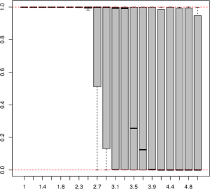
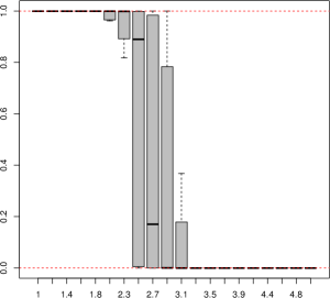
Average sparsity $(\rho=10^{-1.5})$
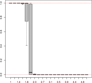
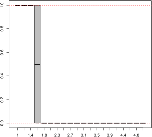
Low sparsity $(\rho=10^{-1})$

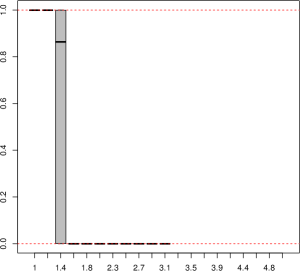
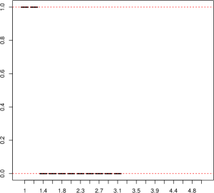
Computational cost.

To give some insight into the computational cost of the proposed methodology, we recorded the running time for the estimation of $p(H_{0}|Y)$, in various conditions. Note that the inference strategy can easily been parallelized. Therefore, to give a fair evaluation, we applied the methodology once for each network generated, on a unique core. The results presented in Table 1 were obtained on an Intel Xeon CPU 3.07GHz, for $\lambda=2$ and $\rho=10^{-1}$. As expected, the running time increases as the network size $n$ becomes higher. Similarly, increasing the number $d$ of covariates induces an additional computational effort. Again, the methodology proposed involves testing various values of $K$ (from $1$ to $10$ in these experiments) which can be done in parallel to reduce significantly the running times. If a core is used for each value of $K$, then the running time is given essentially by the slowest run, usually for the largest value of $K$. For information, the corresponding running times are also indicated in parenthesis in Table 1.

size of the network ($n$)	$d=2$	$d=5$	$d=10$
100	0.47 (0.1)	0.6 (0.12)	0.72 (0.14)
250	3.42 (0.73)	4.74 (0.88)	5.97 (1.26)
500	18.03 (3.73)	20.28 (4.17)	24.43 (4.91)

Table 1: Averaged running times (in minutes) for the estimation of $p(H_{0}|Y)$, for various sizes $n$ of networks and various values of $d$. In parenthesis, the averaged running times (in minutes) for $K=10$.

5 Illustrations

We applied our approach to analyze a series of networks of various sizes and densities, from social sciences and ecology. For all studies, equal prior probabilities were given for the Models $M_{K}$ ($K\geq 2$) such that $p(H_{1}^{\prime})=1/2$. Moreover, we set $a_{0}=b_{0}=c_{0}=d_{0}=e_{0}=1$. The variational algorithm was run on each network for $K$ between $1$ and $16$. For each $K$, the procedure was repeated $20$ times and the run maximizing the lower bound was selected.

Coding of the covariates.

The model we propose involves a regression term $x_{ij}^{\intercal}\beta$ where $x_{ij}$ is a vector of covariates for edge $(i,j)$. In some situations, edge descriptors $x_{ij}$, such as (phylogenetic, geographic) distances, are actually available. But in many situations, only node descriptors $x_{i}$ and $x_{j}$ are available and building an edge descriptor $x_{ij}$ from node descriptors is not a straightforward task (see e.g. Hunter et al., 2008). For all networks (except the blog network to be consistent with Latouche and Robin (2015)), we adopted the following coding rules. Quantitative edge descriptors were treated as quantitative regressors. For quantitative node descriptors, the absolute difference $x_{ij}=|x_{i}-x_{j}|$ was used as a quantitative covariate. For ordinal node descriptors $x_{i}\in\{1,\dots L\}$, we considered the absolute difference $|x_{i}-x_{j}|$ but we treated it as a factor, with $L-1$ levels. Qualitative node descriptors with $L$ levels were transformed into qualitative edge descriptors with $2L$ levels, each node level $\ell$ giving rise to two edge levels: one indicating if both $i$ and $j$ have level $\ell$ and one indicating if either $i$ or $j$ (but not both) has level $\ell$.

5.1 Description of the datasets

Blog network.

The network is made of 196 vertices and was built from a single day snapshot of political blogs extracted on 14th October 2006 (Zanghi et al., 2008). Nodes correspond to blogs and an edge connect two nodes if there is an hyperlink from one blog to the other. They were annotated manually by the “Observatoire Présidentiel” project such that, for each node, labels are available. Thus, each node is associated to a political party from the left wing to the right wing and the status of the writer is also given (political analyst or not). This data set has been studied in a series of works (Zanghi et al., 2008; Latouche et al., 2011, 2014) where all the authors pointed out the crucial role of the labels in the construction of the network. We considered a set of three covariates $x_{ij}=(x_{ij}^{1},x_{ij}^{2},x_{ij}^{3})\in\mathbb{R}^{3}$ artificially constructed to analyze the influence of both the political parties and the writer status. We set $x_{ij}^{1}=1$ if blogs $i$ and $j$ have the same labels, 0 otherwise. Moreover, $x_{ij}^{2}=1$ if one of the two blogs $i$ and $j$ is written by political analysts, $0$ otherwise. Finally, $x_{ij}^{3}=1$ if both are written by political analysts, $0$ otherwise.

Tree network.

This data set was first introduced by Vacher et al. (2008) and further studied in Mariadassou et al. (2010). We considered the tree network which describes the interactions between $51$ trees where two trees interact if they share at least one common fungal parasite. Three quantitative edge descriptors are available characterizing the genetic, geographic, and taxonomic distances between the tree species.

Karate network.

The karate data set describes the friendships between a subset of 34 members of a karate club at a university in the US, observed from 1970 to 1972. It was originally studied by Zachary (1977). When the study started, an incident occurred between the club president and a karate instructor, over the price of the karate lessons. The entire club then became divided over this issue, as time passed. The network is made of four known groups characterized by a node qualitative descriptor, taking four possible values, for each node in the network.

Florentine marriage network.

We considered the data set analyzed by Breiger and Pattison (1981) in their study of local role analysis in social networks. It characterizes the social relations among 16 Renaissance Florentine families and was built by John Padgett from historical documents. Two nodes are linked is the two families share marriage alliances. Three quantitative node covariates are provided for each family, namely the family’s net wealth in 1472 in thousands of lira, the family’s number of seats on the civic councils held between 1282 and 1344, and the family’s total number of business and marriage ties in the entire data set.

Florentine business network.

This data set is similar to the Florentine marriage network described previously except that edges now describe business ties between families. We considered exactly the same covariates.

Faux Dixon High network.

Contrary to all networks presented in this work, this data set is directed and therefore we employed the inference algorithm for the directed case, as presented in the supplementary materials. This network characterizes the (directed) friendship between 248 students. It results from a simulation based upon an exponential random graph model fit (Handcock et al., 2008) to data from one school community from the AddHealth Study, Wave I (Resnick et al., 1997). Node covariates are provided, namely the grade, sex, and race of each student. The grade ordinal attribute has values 7 to 12, indicating each student’s grade in school. Moreover, the race qualitative attributes can take 4 values.

CKM.

This data set was created by Burt (1987) from the data originally collected by Coleman et al. (1966). The network we considered characterizes the friendship relationships among physicians, each physician being asked to name three friends. The physicians were also asked to answer to a series of questions regarding their profession. We focused here on 13 questions corresponding to node covariates among which four are qualitative descriptors: city of practices (4 values), discussion with other doctors (3 values), speciality in a field of medicine (4 values), proximity with other physicians (4 values). All other node covariates were treated as quantitative variables. Note that we imputed the missing values in the data set using the missMDA R package (Josse and Husson, 2016).

AddHealth 67.

This data set is related to the Faux Dixon network described previously. However, it was constructed from the original data of the AddHealth study, and not simulated from any random graph model. The AddHealth study was conducted using in-school questionnaires, from 1994 to 1995. Students were asked to designate their friends and to answer to a series of questions. Results were collected in schools from 84 communities. In our study, we considered a network associated to school community 67 which characterizes the undirected friendship relationships between 530 students. As for the Faux Dixon network, three node covariates are available. The sex qualitative covariate takes two values. Moreover, the grade ordinal attribute has values from 7 to 12. However, contrary to the Faux Dixon network, five values are present in the data for the race qualitative attribute.

5.2 Results

Network	size ($n$)	nb. covariates ($d$)	density	$\hat{p}(H_{0}|Y)$
Blog	196	3	0.075	3.60e-172
Tree	51	3	0.54	2.36e-115
Karate	34	8	0.14	3.38e-2
Florentine (marriage)	16	3	0.17	0.995
Florentine (business)	16	3	0.125	0.991
Faux Dixon High	248	17	0.02	1
CKM	219	39	0.015	1
AddHealth 67	530	21	0.007	2.10e-25

Table 2: Estimation of $p(H_{0}|Y)$, for the eight networks considered.

The estimated values of $p(H_{0}|Y)$ for all networks are presented in Table 2. For illustration purposes, the estimations of the residual structures $g\circ\hat{\phi}$ are also provided in Figures 2, 3, and 4. In practice, we used Proposition 10 to estimate $\hat{\phi}$ and then applied $g(\cdot)$ to obtain graphon-like surfaces. There is no standard definition of $W$-graph models in the directed case and therefore, for the Faux dixon high network, only the estimation of $p(H_{0}|Y)$ is given.

As shown in Table 2, Model $H_{0}$ was rejected for the blog, tree, karate and AddHealth networks. Indeed, we obtained values of $\hat{p}(H_{0}|Y)$ close to zero for the four data sets, indicating that the corresponding covariates cannot explain entirely the construction of these networks. For the blog network, we can observe in Figure 2 (top right) that $g\circ\hat{\phi}$ is not constant which is coherent with Model $H_{0}$ being rejected. We also give in this figure (top left) the estimated residual structure without taking the covariates into account ($d=0$). Clearly, the shape of $g\circ\hat{\phi}$ is simpler when $d=3$. In particular, many of the hills on the diagonal vanish when adding the covariates. Thus, the covariates help in studying and explaining parts of the network. However, they are not sufficient and some of the heterogeneity observed in the network cannot be explained by political parties and writer status. Similar conclusions can be drawn from the tree , karate, and AddHealth networks (Figure 2 and Figure 3). Indeed, the terms $g\circ\hat{\phi}$ simplify when adding the covariates but remain non constant. In particular, for the tree network considered, this means that the interactions between trees through common fungal parasite cannot be entirely explained by the distances available which is consistent with a these from Mariadassou et al. (2010) who describe a residual heterogeneity in the valued version of this network, after taking the covariates into account.

For all other networks considered, model $H_{0}$ was chosen. Indeed, for the Florentine marriage and business networks, we found $\hat{p}(H_{0}|Y)=0.995$ and $\hat{p}(H_{0}|Y)=0.991$ respectively. As expected, the residual structures $g\circ\hat{\phi}$ were found constant when adding the covariates (Figure 4). Moreover, the variational approach led to $\hat{p}(H_{0}|Y)=1$, for the Faux Dixon High and CKM networks. Thus, the statistical framework we propose shows that no other effect than these of the covariates contributes significantly to explain the structure of these networks. In other words, once corrected for the covariates, no residual heterogeneity is observed among the interactions.

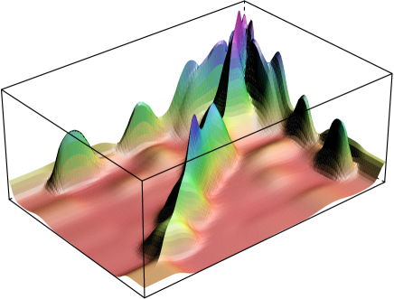
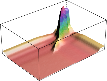
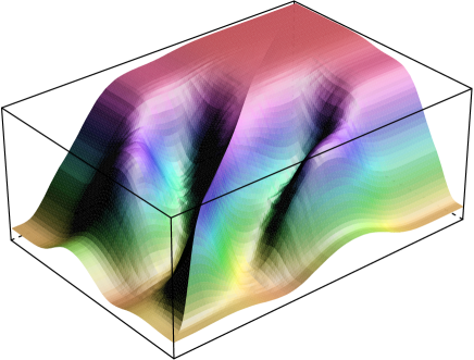
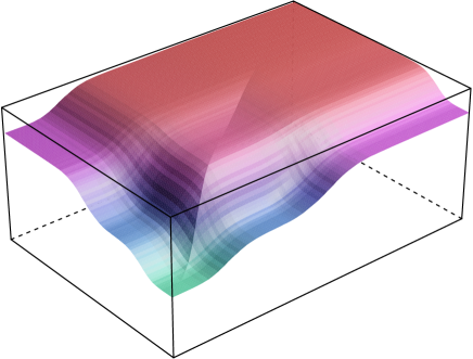
Figure 2: Estimation of the blog (top) and tree (bottom) networks residual structure without (left) and with (right) covariates.

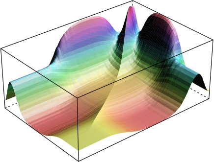
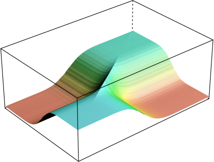
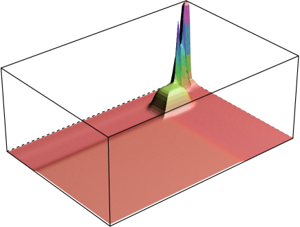
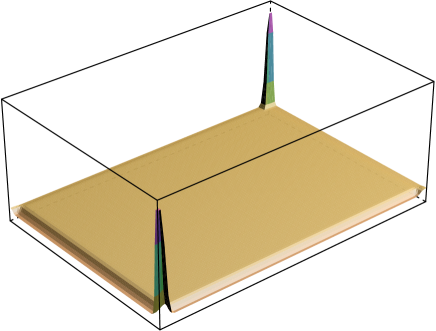
Figure 3: Estimation of the karate (top) and AddHealth (bottom) networks residual structure without (left) and with (right) covariates.

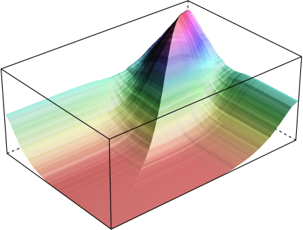
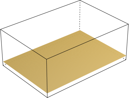
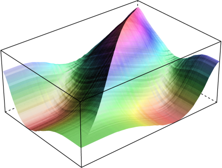
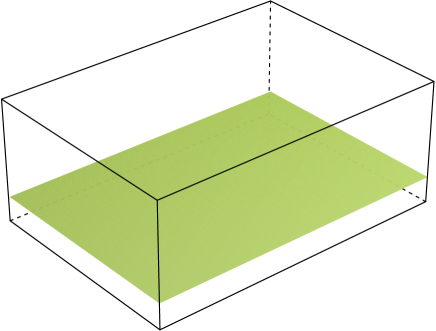
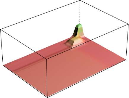
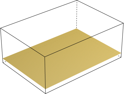
Figure 4: Estimation of the Florentine marriage (top), Florentine business (middle), and CKM networks residual structure without (left) and with (right) covariates.

6 Conclusion

In this paper we proposed a framework to assess the goodness of fit of logistic models for binary networks. Thus, we added a generic term, related to the graphon function of $W$-graph models, to the logistic regression model. The corresponding new model was approximated with a series of models with blockwise constant residual structure. A Bayesian procedure was then considered to derive goodness-of-fit criteria. All these criteria depend on marginal likelihood terms for which we did provide estimates relying on variational approximations. The first approximation was obtained using a variational decomposition while the second involves a series of Taylor expansions. The approach was tested on toy data sets and encouraging results were obtained. Finally, it was used to analyze eight networks from social sciences and ecology. We believe the methodology has a large spectrum of applications since covariates are often given when analyzing binary networks.

Appendix:

Give all proofs of the paper. (Appendix.pdf)

Directed case:

Describe the inference procedure for the directed case. (Directed.pdf)

References

- Airoldi et al. (2013) Airoldi, E. M., T. B. Costa, and S. H. Chan (2013). Stochastic blockmodel approximation of a graphon: Theory and consistent estimation. In Advances in Neural Information Processing Systems, pp. 692–700.
- Albert and Barabási (2002) Albert, R. and A. Barabási (2002). Statistical mechanics of complex networks. Modern Physics 74, 47–97.
- Asta and Shalizi (2014) Asta, D. and C. R. Shalizi (2014). Geometric network comparison. Technical report, arXiv:1411.1350v1.
- Barabási and Oltvai (2004) Barabási, A. and Z. Oltvai (2004). Network biology: understanding the cell’s functional organization. Nature Rev. Genet 5, 101–113.
- Beal and Ghahramani (2002) Beal, M. and Z. Ghahramani (2002). The variational Bayesian em algorithm for incomplete data: with application to scoring graphical model structures. In J. Bernardo, M. Bayarri, J. Berger, A. Dawid, D. Heckerman, A. Smith, and M. e. West (Eds.), Bayesian Statistics 7: Proceedings of the 7th Valencia International Meeting, pp. 453.
- Bishop (2006) Bishop, C. (2006). Pattern recognition and machine learning. Springer-Verlag.
- Bishop and Svensén (2003) Bishop, C. and M. Svensén (2003). Bayesian hierarchical mixtures of experts. In Proceedings of the 19th Conference on Uncertainty in Artificial Intelligence, pp. 57–64. U. Kjaerulff and C. Meek.
- Breiger and Pattison (1981) Breiger, R. and P. Pattison (1981). Cumulated social roles: the duality of persons and their algebras. Social Networks 12, 156–192.
- Burt (1987) Burt, R. (1987). Social contagion and innovation: cohesion versus structural equivalence. American Journal of Sociology 92, 1287–1335.
- Caron and Doucet (2008) Caron, F. and A. Doucet (2008). Sparse Bayesian nonparametric regression. In Proceedings of the 25th International Conference on Machine Learning.
- Chan and Airoldi (2014) Chan, S. and E. Airoldi (2014). A consistent histogram estimator for exchangeable graph models. In T. Jebara and E. P. Xing (Eds.), Proceedings of the 31st International Conference on Machine Learning (ICML-14), pp. 208–216. JMLR Workshop and Conference Proceedings.
- Chatterjee (2015) Chatterjee, S. (2015). Matrix estimation by Universal Singular Value Thresholding. The Annals of Statistics 43(1), 177–214.
- Chung and Lu (2002) Chung, F. and L. Lu (2002). The average distances in random graphs with given expected degrees. Proceedings of the National Academy of Sciences 99, 15879–15882.
- Coleman et al. (1966) Coleman, J., E. Katz, and H. Menzel (1966). Medical innovation: a diffusion study. indianapolis: the boobs-merrill company. Behavioral Science 12, 481–483.
- Dempster et al. (1977) Dempster, A., N. Laird, and D. Rubin (1977). Maximum likelihood for incomplete data via the em algorithm. Journal of the Royal Statistical Society B39, 1–38.
- Diaconis and Janson (2008) Diaconis, P. and S. Janson (2008). Graph limits and exchangeable random graphs. Rend. Mat. Appl. 7(28), 33–61.
- Ducruet (2013) Ducruet, C. (2013). Network diversity and maritime flows. Journal of Transport Geography 30, 77–88.
- Goldenberg et al. (2010) Goldenberg, A., A. Zheng, S. Fienberg, and E. Airoldi (2010). A survey of statistical network models. Foundations and Trends in Machine Learning 2(2), 129–233.
- Handcock et al. (2008) Handcock, M., D. Hunter, C. Butss, S. Goodreau, and M. Morris (2008). Statnet: Software tools for the representation, visualization, analysis and simulation of network data. Journal of Statistical Software 24, 12–25.
- Handcock et al. (2007) Handcock, M. S., A. E. Raftery, and J. M. Tantrum (2007). Model-based clustering for social networks. Journal of the Royal Statistical Society: Series A (Statistics in Society) 170(2), 301–354.
- Hoff (2008) Hoff, P. (2008). Modeling homophily and stochastic equivalence in symmetric relational data. In Advances in Neural Information Processing Systems, pp. 657–664.
- Hoff et al. (2002) Hoff, P. D., A. E. Raftery, and M. S. Handcock (2002). Latent space approaches to social network analysis. Journal of the american Statistical association 97(460), 1090–1098.
- Holland et al. (1983) Holland, P., K. Laskey, and S. Leinhardt (1983). Stochastic blockmodels: some first steps. Social Networks 5, 109–137.
- Hunter et al. (2008) Hunter, D. R., S. M. Goodreau, and M. S. Handcock (2008). Goodness of fit of social network models. Journal of the American Statistical Association 103(481), 248–258.
- Jaakkola and Jordan (2000) Jaakkola, T. and M. Jordan (2000). Bayesian parameter estimation via variational methods. Statistics and Computing 10, 25–37.
- Jeffreys (1946) Jeffreys, H. (1946). An invariant form for the prior probability in estimations problems. In Proceedings of the Royal Society of London. Series A, Volume 186, pp. 453–461.
- Jernite et al. (2014) Jernite, Y., P. Latouche, C. Bouveyron, P. Rivera, L. Jegou, and S. Lamassé (2014). The random subgraph model for the analysis of an acclesiastical network in merovingian gaul. Annals of Applied Statistics 8(1), 377–405.
- Josse and Husson (2016) Josse, J. and F. Husson (2016). missMDA: a package for handling missing values in multivariate data analysis. Journal of Statistical Software 70(1), 1–31.
- Kallenberg (1999) Kallenberg, O. (1999). Multivariate sampling and the estimation problem for exchangeable arrays. Journal of Theoretical Probability 12(3), 859–883.
- Kass and Raftery (1995) Kass, R. E. and A. E. Raftery (1995). Bayes factors. Journal of the american statistical association 90(430), 773–795.
- Lacroix et al. (2006) Lacroix, V., C. Fernandes, and M.-F. Sagot (2006). Motif search in graphs:application to metabolic networks. Transactions in Computational Biology and Bioinformatics 3, 360–368.
- Latouche et al. (2011) Latouche, P., E. Birmelé, and C. Ambroise (2011). Overlapping stochastic block models with application to the french political blogosphere. Annals of Applied Statistics 5(1), 309–336.
- Latouche et al. (2014) Latouche, P., E. Birmelé, and C. Ambroise (2014). Model selection in overlapping stochastic block models. Electronic Journal of Statistics 8(1), 762–794.
- Latouche and Robin (2015) Latouche, P. and S. Robin (2015). Variational Bayes model averaging for graphon functions and motif frequencies inference in -graph models. Statistics and Computing, 1–13.
- Lovász and Szegedy (2006) Lovász, L. and B. Szegedy (2006). Limits of dense graph sequences. Journal of Combinatorial Theory, Series B 96(6), 933 – 957.
- Mariadassou et al. (2010) Mariadassou, M., S. Robin, and C. Vacher (2010). Uncovering latent structure in valued graphs: a variational approach. The Annals of Applied Statistics, 715–742.
- Matias and Robin (2014) Matias, C. and S. Robin (2014). Modeling heterogenity in random graphs through latent space models: a selective review. Esaim Prooceedings and Surveys 47, 55–74.
- Newman (2003) Newman, M. E. J. (2003). The structure and function of complex networks. SIAM Review 45, 167–256.
- Nowicki and Snijders (2001) Nowicki, K. and T. Snijders (2001). Estimation and prediction for stochastic blockstructures. Journal of the American Statistical Association 96, 1077–1087.
- Palla et al. (2010) Palla, G., L. Lovasz, and T. Vicsek (2010, Apr). Multifractal network generator. Proc. Natl. Acad. Sci. U.S.A. 107(17), 7640–7645.
- Snijders and Nowicki (1997) Snijders, T. and K. Nowicki (1997). Estimation and prediction for stochastic block-structures for graphs with latent block structure. Journal of Classification 14, 75–100.
- Vacher et al. (2008) Vacher, C., D. Piou, and M.-L. Desprez-Loustau (2008). Architecture of an antagonistic tree/fungus network: The asymmetric influence of past evolutionary history. PLoS ONE 3(3), 1740. e1740. doi:10.1371/journal.pone.0001740.
- Villa et al. (2008) Villa, N., F. Rossi, and Q. Truong (2008). Mining a medieval social network by kernel som and related methods. Technical report.
- Volant et al. (2012) Volant, S., M.-L. M. Magniette, and S. Robin (2012). Variational Bayes approach for model aggregation in unsupervised classification with markovian dependency. Comput. Statis. & Data Analysis 56(8), 2375 – 2387.
- Wang and Wong (1987) Wang, Y. and G. Wong (1987). Stochastic blockmodels for directed graphs. Journal of the American Statistical Association 82, 8–19.
- Watts and Strogatz (1998) Watts, D. and S. Strogatz (1998). Collective dynamics of small-world networks. Nature 393, 440–442.
- Wolfe and Olhede (2013) Wolfe, P. J. and S. C. Olhede (2013). Nonparametric graphon estimation. Technical report, arXiv:1309.5936.
- Yang et al. (2014) Yang, J. J., Q. Han, and E. M. Airoldi (2014). Nonparametric estimation and testing of exchangeable graph models. In Proceedings of the Seventeenth International Conference on Artificial Intelligence and Statistics, pp. 1060–1067.
- Zachary (1977) Zachary, W. (1977). An information flow model for conflict and fission in small groups. Journal of Anthropological Research 33, 452–473.
- Zanghi et al. (2008) Zanghi, H., C. Ambroise, and V. Miele (2008). Fast online graph clustering via erdös-rényi mixture. Pattern Recognition 41(12), 3592–3599.
- Zanghi et al. (2010) Zanghi, H., S. Volant, and C. Ambroise (2010). Clustering based on random graph model embedding vertex features. Pattern Recognition Letters 31(9), 830–836.
SUPPLEMENTARY MATERIAL