Efficient computation of Bayesian optimal
discriminating designs

Abstract

An efficient algorithm for the determination of Bayesian optimal discriminating designs for competing regression models is developed, where the main focus is on models with general distributional assumptions beyond the “classical” case of normally distributed homoscedastic errors. For this purpose we consider a Bayesian version of the Kullback-Leibler (KL) optimality criterion introduced by López-Fidalgo et al., (2007). Discretizing the prior distribution leads to local KL-optimal discriminating design problems for a large number of competing models. All currently available methods either require a large computation time or fail to calculate the optimal discriminating design, because they can only deal efficiently with a few model comparisons. In this paper we develop a new algorithm for the determination of Bayesian optimal discriminating designs with respect to the Kullback-Leibler criterion. It is demonstrated that the new algorithm is able to calculate the optimal discriminating designs with reasonable accuracy and computational time in situations where all currently available procedures are either slow or fail.

Keyword and Phrases: Design of experiment; Bayesian optimal design; model discrimination; gradient methods; model uncertainty; Kullback-Leibler distance

1 Introduction

Although optimal designs can provide a substantial improvement in the statistical accuracy without making any additional experiments, classical optimal design theory [see for example Pukelsheim, (2006); Atkinson et al., (2007)] has been criticized, because it relies heavily on the specification of a particular model. In many cases a good design for a given model might be inefficient if it is used in a different setup. Most of the literature addressing the problem of model uncertainty in the design of experiments can be roughly divided into two parts, where all authors assume that a certain class of parametric models is available to describe the relation between the predictor and the response. One approach to obtain model robustness is to construct designs which allow the efficient estimation of parameters in all models under consideration. This is usually achieved by optimizing composite optimality criteria, which are defined as an average of the criteria for the different models [see Läuter, (1974), Dette, (1990); Biedermann et al., (2006); Dette et al., (2008)]. Alternatively, one can directly construct designs to discriminate between several competing models. An early reference is Stigler, (1971) who determined designs for discriminating between two nested univariate polynomials by minimizing the volume of the confidence ellipsoid for the parameters corresponding to the extension of the smaller model. Since this seminal paper several authors have followed this line of research [see for example Dette and Haller, (1998) or Song and Wong, (1999) among others]. A completely different approach for the construction of optimal designs for model discrimination was suggested by Atkinson and Fedorov, 1975a . The corresponding optimality criterion is called $T$-optimality criterion. To be precise, assume that the relation between the response $Y$ and predictor $x$ is described by a nonlinear regression model such that

(1.1) $$\mathbb{E}[Y|x]=\eta(x,\theta)~{},~{}\mbox{Var}(Y|x)=v^{2}(x,\theta)~{},$$

and that the experimenter considers two rival models, say $\eta_{1},\eta_{2}$, as candidates for the parametric form of the mean. Roughly speaking, Atkinson and Fedorov, 1975a assumed homoscedasticity, fixed one model, say $\eta_{1}$, and constructed the design such that the sum of squares for a lack of fit test against the alternative $\eta_{2}$ is large. The criterion was extended in several directions. For example, Atkinson and Fedorov, 1975b considered the problem of discriminating a selected model $\eta_{1}$ from a class of other regression models, say $\{\eta_{2},\ldots,\eta_{\nu}\}$, $\nu\geq 2$, and Tommasi, (2009) combined the $T$-criterion with the approach introduced by Läuter, (1974). Ucinski and Bogacka, (2005) remarked that the criterion introduced by Atkinson and Fedorov, 1975a is only applicable in the case of homoscedastic errors in the regression model (1.1) and discussed an extension to the case of heteroscedasticity. More generally, López-Fidalgo et al., (2007) introduced a generalization of the $T$-optimality criterion which is applicable under general distributional assumptions and called KL-optimality criterion. Meanwhile the determination of KL-optimal discriminating designs has been discussed by several authors [see Tommasi, (2009); Tommasi and López-Fidalgo, (2010) among others].
It is important to note here that the $T$-optimality criterion and its extensions are local optimality criteria in the sense of Chernoff, (1953), because they require the explicit knowledge of the parameters in the model $\eta_{1}$. As a consequence, optimal designs with respect to the $T$-optimality criterion might be sensitive with respect to misspecification of the parameters [see Dette et al., (2012) for a striking example]. A standard approach to obtain robust designs [which was already mentioned by Atkinson and Fedorov, 1975a ] is the use of a Bayesian $T$-optimality criterion. This criterion is defined as an expectation of various local $T$-optimality criteria with respect to a prior distribution. Dette et al., (2012) derived some explicit Bayesian $T$-optimal designs for polynomial regression models, but in general these designs have to be found numerically in nearly all cases of practical interest. Recently, Dette et al., (2015) pointed out that the numerical construction of Bayesian $T$-optimal designs is an extremely difficult optimization problem, because – roughly speaking – the Bayesian optimality criterion corresponds to an optimal design problem for model discrimination with an extremely large number of competing models. As a consequence, the commonly used algorithms for the calculation of optimal designs, such as exchange-type methods or multiplicative methods and their extensions, cannot be applied to determine the Bayesian $T$-optimal discriminating design in reasonable computational time. Dette et al., (2015) proposed a new algorithm for the calculation of Bayesian $T$-optimal discriminating designs and demonstrated its efficiency in several numerical examples. A drawback of this method consists still in the fact that it is only applicable to the “classical” Bayesian $T$-optimality criterion which refers to the nonlinear regression model (1.1) with homoscedastic and normally distributed responses, i.e. $\mathbb{P}^{Y|x}\sim\mathcal{N}(\eta(x,\theta),v^{2}(x,\theta))$.

The purpose of the present paper is to extend the methodology introduced by Dette et al., (2015) to regression models with more general distributional assumptions. In Section 2 we will introduce a Bayesian KL-optimality criterion which extends the criterion introduced by López-Fidalgo et al., (2007) to address for uncertainty in the model parameters. The criterion has also been discussed in Tommasi and López-Fidalgo, (2010), who considered only two competing regression models. The new algorithm is proposed in Section 3 and combines some features of the classical exchange type algorithms with gradient methods and quadratic programming. In Section 4 we illustrate the applicability of the new method in several examples. In particular, we determine optimal discriminating designs with respect to the Bayesian KL-optimality criterion in situations where all other methods fail to find the optimal design. Finally, the appendix contains a proof of an auxiliary result.

2 KL-optimal discriminating designs

The regression model (1.1) is a special case of a more general model, where the distribution of the random variable $Y$ has a density, say $f(y,x)$, and $x$ denotes an explanatory variable, which varies in a compact design space $\mathcal{X}$. We assume that observations at different experimental conditions are independent. Following Kiefer, (1974) we consider approximate designs that are defined as probability measures, say $\xi$, with finite support. The support points $x_{1},\ldots,x_{k}$ of a design $\xi$ give the locations where observations are taken, while the weights $\omega_{1},\ldots,\omega_{k}$ describe the relative proportions of observations at these points. If an approximate design is given and $n$ observations can be taken, a rounding procedure is applied to obtain integers $n_{i}$ ($i=1,\ldots,k)$ from the not necessarily integer valued quantities $\omega_{i}n$ such that $\sum_{i=1}^{k}n_{i}=n$.

Assume that the experimenter wants to choose a most appropriate model from a given class, say $\{f_{1},\ldots,f_{\nu}\}$ of competing models, where $f_{j}(y,x,\theta_{j})$ denotes the density of the $j$th model with respect to a sigma-finite measure, say $\mu$. The parameter $\theta_{j}$ varies in a compact parameter space $\Theta_{j}\ (j=1,\dots,\nu)$. The models may contain additional nuisance parameters, which will not be displayed in our notation. For two competing models, say $f_{i}$ and $f_{j}$, we denote by

(2.1) $$I_{i,j}(x,\theta_{i},\theta_{j})=\int f_{i}(y,x,\theta_{i})\log\frac{f_{i}(y,x,\theta_{i})}{f_{j}(y,x,\theta_{j})}\mu(dy)$$

the Kullback-Leibler distance between $f_{i}$ and $f_{j}$. If the model $f_{i}$ is assumed to be the “true” model with parameter $\overline{\theta}_{i}$, then López-Fidalgo et al., (2007) defined a local KL-optimal discriminating design for the models $f_{i}$ and $f_{j}$ as a design maximizing the optimality criterion

(2.2) $$\mathrm{KL}_{i,j}(\xi,\overline{\theta}_{i})=\inf_{\theta_{i,j}\in\Theta_{j}}\int_{\mathcal{X}}I_{i,j}(x,\overline{\theta}_{i},\theta_{i,j})\xi(dx).$$

This criterion can now easily be extended to construct optimal discriminating designs for more than two competing models. Following Tommasi and López-Fidalgo, (2010) and Braess and Dette, (2013) we denote by $p_{i,j}$ nonnegative weights reflecting the importance of the comparison between the the model $f_{i}$ and $f_{j}$, where $f_{i}$ is assumed as the “true” model. The (symmetrized) KL-optimality criterion for more than $\nu\geq 2$ competing models $f_{1},\dots,f_{\nu}$ is then defined by

(2.3) $$\mathrm{KL}_{\mathrm{P}}(\xi)=\sum_{i,j=1}^{\nu}p_{i,j}\mathrm{KL}_{i,j}(\xi,\overline{\theta}_{i})=\sum_{i,j=1}^{\nu}p_{i,j}\inf_{\theta_{i,j}\in\Theta_{j}}\int_{\mathcal{X}}I_{i,j}(x,\overline{\theta}_{i},\theta_{i,j})\xi(dx),$$

and a design maximizing the criterion (2.3) is called local $\mathrm{KL}_{\mathrm{P}}$-optimal discriminating design for the models $f_{1},\ldots,f_{\nu}$. For a design $\xi$ we also introduce the notation

(2.4) $${\Theta}_{i,j}^{*}(\xi)=\operatorname*{arg\,inf}_{\theta_{i,j}\in\Theta_{j}}\int_{\mathcal{X}}I_{i,j}(x,\overline{\theta}_{i},\theta_{i,j})\xi(dx),$$

Our first result characterizes local KL-optimal discriminating design and will be helpful to check the optimality of the numerically constructed designs. Its proof can be obtained by standard arguments and is therefore omitted.

Theorem 2.1

Let

• Assumption 2.1

  For each $i=1,\dots,\nu$ the function $f_{i}(\cdot,\cdot,\theta_{i})$ is continuously differentiable with respect to the parameter $\theta_{i}\in\Theta_{i},$

be satisfied. A design $\xi^{*}$ is a local $\mathrm{KL}_{\mathrm{P}}$-optimal discriminating design, if and only if there exist distributions $\rho_{ij}^{*}$ on the sets ${\Theta}_{i,j}^{*}(\xi^{*})$ defined in (2.4) such that the inequality

(2.5) $$\sum_{i,j=1}^{\nu}p_{i,j}\int_{{\Theta}_{i,j}^{*}(\xi^{*})}I_{i,j}(x,\overline{\theta}_{i},\theta_{i,j})\rho_{ij}^{*}(d{\theta}_{i,j})~{}\leq\mathrm{KL}_{\mathrm{P}}(\xi^{*})$$

is satisfied for all $x\in\mathcal{X}$. Moreover, there is equality in (2.5) for all support points of the local $\mathrm{KL}_{\mathrm{P}}$-optimal discriminating design $\xi^{*}$.

If, additionally,

• Assumption 2.2

  For any design $\xi$ such that $\mathrm{KL}_{\mathrm{P}}(\xi)>0$ and weight $p_{i,j}\neq 0$ the infima in (2.3) are attained at a unique points $\widehat{\theta}_{i,j}=\widehat{\theta}_{i,j}(\xi)$ in the interior of the set $\Theta_{j}$,

is satisfied, then all measures $\rho_{ij}^{*}$ in Theorem 2.1 are one-point measures and the left-hand side of inequality (2.5) simplifies to

(2.6) $$\Psi(x,\xi)=\sum_{i,j=1}^{\nu}p_{i,j}I_{i,j}(x,\overline{\theta}_{i},\widehat{\theta}_{i,j}).$$

Consequently, if $\xi$ is not a local $\mathrm{KL}_{\mathrm{P}}$-optimal discriminating design, it follows that there exists a point $\bar{x}\in\mathcal{X}$ such that $\Psi(\bar{x},\xi)>\mathrm{KL}_{\mathrm{P}}(\xi)$.

Note that the criterion (2.3) depends on the unknown parameters $\overline{\theta}_{1},\ldots,\overline{\theta}_{\nu}$, which have to be specified by the experimenter for the competing model $f_{1},\dots,f_{\nu}$, respectively. Therefore the criterion is a local one in the sense of Chernoff, (1953). It was pointed out by Dette et al., (2012) that the optimal designs maximizing the criterion (2.3) are rather sensitive with respect to misspecification of these parameters. For this reason we will now propose a Bayesian version of the criterion in order to obtain robust discriminating designs for the competing models $f_{1},\ldots,f_{\nu}$.
We denote by $\mathcal{P}_{i}$ a prior distribution for the parameter $\overline{\theta}_{i}$ in model $f_{i}$ ($i=1,\ldots,\nu$) and define a Bayesian KL-optimality criterion by

(2.7) $$\mathrm{KL}_{\mathrm{P}}^{\mathrm{B}}(\xi) =\sum_{i,j=1}^{\nu}p_{i,j}\int_{\Theta_{i}}\mathrm{KL}_{i,j}(\xi,\overline{\theta}_{i})\mathcal{P}_{i}(d\overline{\theta}_{i}),$$

$$=\sum_{i,j=1}^{\nu}p_{i,j}\int_{\Theta_{i}}\inf_{\theta_{i,j}\in\Theta_{j}}\int_{\mathcal{X}}I_{i,j}(x,\overline{\theta}_{i},\theta_{i,j})\xi(dx)\mathcal{P}_{i}(d\overline{\theta}_{i})$$

Optimal designs maximizing this criterion will be called Bayesian KL-optimal discriminating designs throughout this paper. We also note that the criterion (2.7) has been considered before by Tommasi and López-Fidalgo, (2010) in the case of two competing regression models.
It was pointed out by Dette et al., (2015) that the determination of Bayesian optimal discriminating designs with respect to the criterion (2.7) is closely related to the problem of finding local optimal discriminating designs for a large class of competing regression models. To be precise, we note that in most applications the integral in (2.7) is evaluated by numerical integration approximating the prior distribution by a measure with finite support. Consequently, if the prior distribution $\mathcal{P}_{i}$ in the criterion is given by a discrete measure with masses $\tau_{i1},\ldots\tau_{i\ell_{i}}$ at the points $\lambda_{i1},\ldots,\lambda_{i\ell_{i}}$ the criterion in (2.7) can be represented as

(2.8) $$\mathrm{KL}_{\mathrm{P}}^{\mathrm{B}}(\xi)=\sum_{i,j=1}^{\nu}\sum_{k=1}^{\ell_{i}}p_{i,j}\tau_{ik}\inf_{\theta_{i,j}\in\Theta_{j}}\int_{\mathcal{X}}I_{i,j}(x,{\lambda_{ik}},\theta_{i,j})\xi(dx).$$

which is a local KL-optimality criterion of the from (2.3), where the competing models are given by $\{f_{i}(y,x,\lambda_{ik})|~{}k=1,\dots,\ell_{i};\ i=1,\dots,\nu\}$. The only difference between the criterion obtained from the (discrete) Bayesian approach and the criterion (2.3) consists in the fact that - due to discretization of the prior distributions $\mathcal{P}_{1},\ldots,\mathcal{P}_{\nu}$ - the criterion (2.8) involves substantially more comparisons of competing models $f_{i}(y,x,\lambda_{ik})$. As a consequence the computation of Bayesian KL-optimal discriminating design is computationally very challenging, because for each support point of the prior distribution in the criterion (2.8) the infimum has to be calculated numerically. In the following section we will propose several new algorithms to address this problem. In Section 4 it will be demonstrated that these methods yield very satisfactory results in cases where commonly used algorithms are either very slow or fail to determine the Bayesian KL-optimal discriminating design.

3 Efficient algorithms for Bayesian KL-optimal designs

In this section we propose several algorithms for the calculation of Bayesian KL-optimal designs, which determine the optimal designs with reasonable accuracy and are computationally very efficient. As pointed out in Section 2 the Bayesian optimality criterion with a discrete prior distribution reduces to a local KL-optimality criterion of the form (2.3) with a large number of model comparisons. For this reason we will describe the numerical procedures in this section for the criterion (2.3). It is straightforward to extend the algorithms to the Bayesian criterion (2.8) and in the following Section 4 we will give some illustrations determining Bayesian KL-optimal discriminating designs by the new methods.

Most of the algorithms proposed in the literature for the calculation of optimal designs are based on the fact which was mentioned in the paragraph following Theorem 2.1. More precisely, recall the definition of the function $\Psi$ in (2.6) and assume that the design $\xi$ is not a Bayesian KL-optimal discriminating design. It then follows under Assumption 2.2 that there exists a point $\overline{x}\in\mathcal{X}$, such that the inequality

$$\Psi(\overline{x},\xi)>\mathrm{KL}_{\mathrm{P}}(\xi)$$

holds. López-Fidalgo et al., (2007) used this property to extend the algorithm of Atkinson and Fedorov, 1975a to the KL-optimality criterion. In the case of the local KL-optimality criterion (2.3) it reads as follows.

Algorithm 3.1

Let $\xi_{0}$ denote a given (starting) design and let $(\alpha_{s})_{s=0}^{\infty}$ be a sequence of positive numbers, such that $\lim_{s\to\infty}\,\alpha_{s}=0,\;\sum_{s=0}^{\infty}\alpha_{s}=\infty,\;\sum_{s=0}^{\infty}\alpha_{s}^{2}<\infty.$ For $s=0,1,\ldots$ define

$$\xi_{s+1}=(1-\alpha_{s})\xi_{s}+\alpha_{s}\xi(x_{s+1}),$$

where $x_{s+1}=\operatorname*{arg\,max}_{x\in\mathcal{X}}\Psi(x,\xi_{s}).$

It can be shown that this algorithm yields a sequence of designs $(\xi_{s})_{s\in\mathbb{N}}$ converging in the sense that $\lim_{s\to\infty}\mathrm{KL}_{\mathrm{P}}(\xi_{s})=\mathrm{KL}_{\mathrm{P}}(\xi^{*})$, where $\xi^{*}$ denotes a local KL-optimal discriminating design. However, it turns out that the rate of convergence is very slow. In particular, if there are many models under consideration, the algorithm is very slow and fails in some models to determine the local KL-optimal discriminating design (see our numerical example in Section 4). One reason for these difficulties consists in the fact that Algorithm 3.1 usually yields a sequence of designs with an increasing number of support points. As a consequence the resulting design (after applying some stopping criterion) is concentrated on a large set of points. In the case of normal distributed responses it is also demonstrated by Braess and Dette, (2013) that Algorithm 3.1 requires a large number of iterations if it is used for the calculation of local KL-optimal discriminating designs for more than two competing models.

Following Dette et al., (2015) we therefore propose an alternative procedure for the calculation of local KL-optimal discriminating designs, which separates the maximization with respect to the support points and weights in two steps. In the discussion below we will present two methods for the calculation of the weights in the second step [see Section 3.1 and 3.2 for details].

Algorithm 3.2

Let ${\xi_{0}}$ denote a starting design such that $\mathrm{KL}_{\mathrm{P}}({\xi_{0}})>0$ and define recursively a sequence of designs $({\xi_{s}})_{s=0,1,\ldots}$ as follows:

• Let $\mathcal{S}_{[s]}$ denote the support of the design ${\xi_{s}}$. Determine the set $\mathcal{E}_{[s]}$ of all local maxima of the function $\Psi(x,{\xi_{s}})$ on the design space $\mathcal{X}$ and define $\mathcal{S}_{[s+1]}=\mathcal{S}_{[s]}\cup\mathcal{E}_{[s]}$.

• Define $\xi=\{\mathcal{S}_{[s+1]},\omega\}$ as the design supported at $\mathcal{S}_{[s+1]}$ (with a normalized vector $w$ of non-negative weights) and determine the local $\mathrm{KL}_{\mathrm{P}}$-optimal design in the class of all designs supported at $\mathcal{S}_{[s+1]}$. In other words: we determine the vector $\omega_{[s+1]}$ maximizing the function

  $$g(\omega)=\mathrm{KL}_{\mathrm{P}}(\{\mathcal{S}_{[s+1]},\omega\})=\sum_{i,j=1}^{\nu}p_{i,j}\inf_{\theta_{i,j}\in\Theta_{j}}\sum_{x\in\mathcal{S}_{[s+1]}}I_{i,j}(x,\overline{\theta}_{i},\theta_{i,j})w_{x}$$

  (here $w_{x}$ denotes the weights at the point $x\in\mathcal{S}_{s+1}$). All points in ${\mathcal{S}}_{[s+1]}$ with vanishing components in the vector of weights $\omega_{[s+1]}$ will be be removed and the new set of support points will also be denoted by ${\mathcal{S}}_{[s+1]}$. Finally the design ${\xi}_{s+1}$ is defined as the design with the set of support points ${\mathcal{S}}_{[s+1]}$ and the corresponding nonzero weights.

It follows by similar arguments as given in Dette et al., (2015) that the sequence $({\xi_{s}})_{s=0,1,\ldots}$ of designs generated by Algorithm 3.2 converges to a local KL-optimal discriminating design. The crucial step in this algorithm is the second one, because it requires – in particular if a large number of competing models are under consideration – the calculation of numerous infima. In order to address this problem we propose a quadratic programming and a gradient method in the following two subsections.

3.1 Quadratic programming

Let $\mathcal{S}_{[s+1]}=\{x_{1},\ldots,x_{n}\}$ denote the set obtained in the first step of Algorithm 3.2 and recall the definition of the Kullback-Leibler distance $I_{i,j}$ in (2.1). In Step 2 of Algorithm 3.2 a design $\xi$ with masses $\omega_{1},\ldots,\omega_{n}$ at the points $x_{1},\ldots,x_{n}$ has to be determined such that the function

$$g(\omega)=\sum_{i,j=1}^{\nu}p_{i,j}\sum_{k=1}^{n}\omega_{k}\int\log\Big{\{}\frac{f_{i}(y,x_{k},\overline{\theta}_{i})}{f_{j}(y,x_{k},\widehat{\theta}_{i,j})}\Big{\}}f_{i}(y,x_{k},\overline{\theta}_{i})d\mu(y).$$

is maximal, where

(3.1) $$\widehat{\theta}_{i,j}=\widehat{\theta}_{i,j}(\omega)=\operatorname*{arg\,inf}_{\theta_{i,j}\in\Theta_{j}}\sum_{k=1}^{n}\omega_{k}\int\log\left\{\frac{f_{i}(y,x_{k},\overline{\theta}_{i})}{f_{j}(y,x_{k},{\theta}_{i,j})}\right\}f_{i}(y,x_{k},\overline{\theta}_{i})~{}.$$

Define

$$\mathbf{J}_{i,j}(y) =\mathbf{J}_{i,j}(\widehat{\theta}_{i,j},y)=\left(\frac{\sqrt{f_{i}(y,x_{k},\overline{\theta}_{i})}}{f_{j}(y,x_{k},\widehat{\theta}_{i,j})}\frac{\partial f_{j}(y,x_{k},\theta_{i,j})}{\partial\theta_{i,j}}\Big{|}_{{\theta}_{i,j}=\widehat{\theta}_{i,j}}\right)_{k=1}^{n}\in\mathbb{R}^{n\times d_{j}},$$

$$\mathbf{R}_{i,j} =\mathbf{R}_{i,j}(\widehat{\theta}_{i,j})=\left(\int\frac{\partial f_{j}(y,x_{k},\theta_{i,j})}{\partial\theta_{i,j}}\Big{|}_{{\theta}_{i,j}=\widehat{\theta}_{i,j}}\frac{f_{i}(y,x_{k},\overline{\theta}_{i})}{f_{j}(y,x_{k},\widehat{\theta}_{i,j})}d\mu(y)\right)_{k=1}^{n}\in\mathbb{R}^{n\times d_{j}},$$

and consider a linearized version of the function $g$, that is

(3.2) $$\overline{g}(\omega)=\sum_{i,j=1}^{\nu}p_{i,j}\min_{\alpha_{i,j}}\sum_{k=1}^{n}\omega_{k}\left\{\int\log\left\{\frac{f_{i}(y,x_{k},\overline{\theta}_{i})}{f_{j}(y,x_{k},{{\widehat{\theta}_{i,j}})}}\right\}f_{i}(y,x_{k},\overline{\theta}_{i})d\mu(y)\right.$$

$$+\left.\alpha_{i,j}^{T}(\mathbf{R}_{i,j}^{T})_{k}-\frac{1}{2}\int\alpha_{i,j}^{T}(\mathbf{J}^{T}_{i,j}(y))_{k}(\mathbf{J}_{i,j}(y))_{k}\alpha_{i,j}d\mu(y)\right\}.$$

Note that the minimum with respect to the parameters $\alpha_{i,j}\in\mathbb{R}^{d_{j}}$ is achieved for

$$\widehat{\alpha}_{i,j}=\left(\int\mathbf{J}_{i,j}^{T}(y)\mathbf{\Omega}\mathbf{J}_{i,j}(y)d\mu(dy)\right)^{-1}\mathbf{R}_{i,j}^{T}\omega,$$

where the matrix $\mathbf{\Omega}$ is defined by $\mathbf{\Omega}=\mbox{diag}(\omega_{1},\dots,\omega_{n})$ and $\omega=(\omega_{1},\dots,\omega_{n})^{T}$. For the following discussion we define by $\Delta=\{\omega\in\mathbb{R}^{n}~{}|~{}\omega_{i}\geq 0~{}(i=1,\ldots,n)\;\sum_{i=1}^{n}\omega_{i}=1\}$ the simplex in $\mathbb{R}^{n}$.

Lemma 3.3

If Assumptions 2.1 and 2.2 are satisfied, then each maximizer of the function $g(\cdot)$ in $\Delta$ is a maximizer of $\overline{g}(\cdot)$ in $\Delta$ and vice versa. Moreover,

$$\max_{\omega\in\Delta}g(\omega)=\max_{\omega\in\Delta}\overline{g}(\omega).$$

A proof of Lemma 3.3 can be found in the Section 5. With the notations

$$\mathbf{b}_{i,j}=\mathbf{b}_{i,j}({\widehat{\theta}_{i,j}})=\left(\int\log\left\{\frac{f_{i}({y,x_{k}},\overline{\theta}_{i})}{f_{j}({y,x_{k}},{\widehat{\theta}_{i,j}})}\right\}f_{i}({y,x_{k}},\overline{\theta}_{i}){\mu(dy)}\right)_{k=1}^{n}{=\left(I_{i,j}(x_{k},\overline{\theta}_{i},\widehat{\theta}_{i,j})\right)_{k=1}^{n}}~{}\in\mathbb{R}^{n}$$

we have

$$\overline{g}(\omega)=\mathbf{b}^{T}\omega-\omega^{T}\mathbf{Q}(\omega)\omega$$

where the vector $\mathbf{b}\in\mathbb{R}^{n}$ and the $n\times n$ matrix $\mathbf{Q}$ are defined by

$$\mathbf{Q}(\omega)=\mathbf{R}_{i,j}\left(\int\mathbf{J}_{i,j}^{T}(y)\mathbf{\Omega}(\omega)\mathbf{J}_{i,j}(y){\mu(dy)}\right)^{-1}\mathbf{R}_{i,j}^{T},$$

and $\mathbf{b}=\Sigma^{\nu}_{i,j=1}p_{i,j}\mathbf{b}_{i,j}$, respectively. If we ignore the dependence of the matrix $\mathbf{Q}(\omega)$ and consider this matrix as fixed for a given matrix $\mathbf{\Omega}=\mathrm{diag}(\overline{\omega}_{1},\dots,\overline{\omega}_{n})$, we obtain a quadratic programming problem, that is

(3.3) $$\phi(\omega,\overline{\omega})=-\omega^{\mathrm{T}}\mathbf{Q(\overline{\omega})}\;\omega+\mathbf{b}^{\mathrm{T}}\omega\rightarrow\max_{\omega\in\Delta}.$$

This problem can now be solved iteratively substituting each time the solution obtained in the previous iteration instead of $\overline{\omega}$.

Example 3.4

In this example we illustrate the calculation of the function $\mathbf{Q}(\omega)$ under several distributional assumptions.

• Ucinski and Bogacka, (2005) considered the regression model with normal distributed heteroscedastic errors, that is

  $$f(y,x,\theta)=\frac{1}{\sqrt{2\pi v^{2}(x,\theta)}}\exp\Bigl{(}-\frac{(y-\eta(x,\theta))^{2}}{2v^{2}(x,\theta)}\Bigr{)},$$

  where $\eta(x,\theta)$ and $v^{2}(x,\theta)$ denotes the expectation and variance of the response at experimental condition $x$. In this case the Kullback-Leibler distance between the two densities $f_{i}$ and $f_{j}$ is given by

  $$I_{i,j}({x},\overline{\theta}_{i},{\theta}_{i,j})=\frac{\left[\eta_{i}(x,\overline{\theta}_{i})-\eta_{j}(x,\theta_{i,j})\right]^{2}}{v_{j}^{2}(x,\theta_{i,j})}+\frac{v_{i}^{2}(x,\overline{\theta}_{i})}{v_{j}^{2}(x,\theta_{i,j})}+\log\left\{\frac{v_{j}^{2}(x,\theta_{i,j})}{v_{i}^{2}(x,\theta_{i})}\right\}-1,$$

  and a straightforward calculation gives for the function $\bar{g}$ in (3.2) the representation

  $$\overline{g}(\omega) =\sum_{i,j=1}^{\nu}\min_{\alpha_{i,j}}\left[\alpha_{i,j}^{T}\mathbf{J}_{i,j}^{T}\mathbf{\Omega}_{i}\mathbf{J}_{i,j}\alpha_{i,j}+2\omega^{T}\mathbf{R}_{i,j}\alpha_{i,j}+\mathbf{b}_{i,j}^{T}\omega\right],$$

  where $\mathbf{\Omega}_{i}=\mbox{diag}\left(\omega_{1},\dots,\omega_{n}\right),$

  $$s_{i,j}(x,\theta_{i,j})=\frac{v_{i}^{2}(x,\theta_{i})}{v_{j}^{2}(x,\theta_{i,j})}+\log\left\{\frac{v_{j}^{2}(x,\theta_{i,j})}{v_{i}^{2}(x,\theta_{i})}\right\};\;h_{i,j}(x,\theta_{i,j})=\frac{\eta_{i}(x,\theta_{i})-\eta_{j}(x,\theta_{i,j})}{v_{j}(x,{\theta}_{i,j})};$$

  $$\mathbf{J}_{i,j}=\left(\frac{\partial h_{i,j}(x_{k},\theta_{i,j})}{\partial\theta_{i,j}}\Big{|}_{\theta_{i,j}=\widehat{\theta}_{i,j}}\right)_{k=1,\dots,n};$$

  $$\mathbf{R}_{i,j}=\left(h_{i,j}(x_{k},\widehat{\theta}_{i,j})\frac{\partial h_{i,j}(x_{k},\theta_{i,j})}{\partial\theta_{i,j}}\Big{|}_{\theta_{i,j}=\widehat{\theta}_{i,j}}+\frac{1}{2}\frac{\partial s_{i,j}(x_{k},\theta_{i,j})}{\partial\theta_{i,j}}\Big{|}_{\theta_{i,j}=\widehat{\theta}_{i,j}}\right)_{k=1,\dots,n};$$

  $$\mathbf{b}_{i,j}=\left(I_{i,j}(x_{k},\overline{\theta}_{i},\widehat{\theta}_{i,j})\right)_{k=1,\dots,n}$$

• López-Fidalgo et al., (2007) considered the regression model (1.1) with log-normal distribution with parameters $\mu(x,\theta)$ and $\sigma^{2}(x,\theta)$. This means that the mean and the variance are given by

  $$\mathbb{E}[Y] = \eta(x,\theta)=\exp\Bigl{\{}\frac{\sigma^{2}(x,\theta)}{2}+\mu(x,\theta)\Bigr{\}},$$

  $$\mbox{Var}(Y) = v^{2}(x,\theta)=\eta^{2}(x,\theta)\{\exp\{\sigma^{2}(x,\theta)\}-1\}~{},$$

  respectively, and the density of the response $Y$ is given by

  $$f(y,x,\theta)=\frac{1}{x\sqrt{2\pi}\sigma(x,\theta)}\exp\Big{\{}-\frac{\left\{\log(y)-\mu(x,\theta)\right\}^{2}}{2\sigma^{2}(x,\theta)}\Big{\}}$$

  In the paper López-Fidalgo et al., (2007) it was shown that the Kullback-Leibler distance between two log-normal densities with parameters $\mu_{\ell}(x,\theta_{\ell})$ and $\sigma_{\ell}^{2}(x,\theta_{\ell})$ ($\ell=i,j$) is given by

  (3.4) $$I_{ij}(x,{\theta}_{i},{\theta}_{i,j})=\frac{1}{2}\Bigl{\{}s_{i,j}(x,\theta_{i,j})+\frac{\left[\mu_{i}(x,\theta_{i})-\mu_{j}(x,\theta_{i,j})\right]^{2}}{\sigma_{i}^{2}(x,\theta_{i})}-1\Bigr{\}},$$

  where

  $$s_{i,j}(x,\theta_{i,j})=\log\Bigl{[}\frac{\sigma_{i}^{2}(x,\theta_{i})}{\sigma_{j}^{2}(x,\theta_{i,j})}\Bigr{]}+\frac{\sigma_{j}^{2}(x,\theta_{i,j})}{\sigma_{i}^{2}(x,\theta_{i})},$$

  and

  $$\sigma_{i}^{2}(x,\theta_{i}) =\log\left[1+v^{2}_{i}(x,\theta_{i})/\eta_{i}^{2}(x,\theta_{i})\right],$$

  $$\mu_{i}(x,\theta_{i}) =\log\left[\eta_{i}(x,\theta_{i})\right]-\sigma^{2}_{i}(x,\theta_{i})/2.$$

  Now a straightforward calculation gives for the function $\bar{g}$ in (3.2) the representation

  $$\overline{g}(\omega) =\frac{1}{2}\sum_{i,j=1}^{\nu}\min_{\alpha_{i,j}}\left[\alpha_{i,j}^{T}\mathbf{J}_{i,j}^{T}\mathbf{\Omega}_{i}\mathbf{J}_{i,j}\alpha_{i,j}-2\omega^{T}\mathbf{R}_{i,j}\alpha_{i,j}+\mathbf{b}_{i,j}^{T}\omega\right],$$

  where $\mathbf{\Omega}_{i}=\mbox{diag}\left(\omega_{1},\dots,\omega_{n}\right)$,

  $$\mathbf{J}_{i,j} =\left(\frac{\frac{\partial\mu_{j}(x_{k},\theta_{i,j})}{\partial\theta_{i,j}}\Big{|}_{\theta_{i,j}=\widehat{\theta}_{i,j}}}{\sigma_{i}(x_{1},\overline{\theta}_{i})}\right)_{k=1,\dots,n};$$

  $$\mathbf{R}_{i,j} =\left(\frac{\big{[}\mu_{i}(x_{k},\overline{\theta}_{i})-\mu_{j}(x_{k},\widehat{\theta}_{i,j})\big{]}\frac{\partial\mu_{i}(x_{k},\theta_{i,j})}{\partial\theta_{i,j}}\big{|}_{\theta_{i,j}=\widehat{\theta}_{i,j}}}{\sigma^{2}_{i}(x_{k},\overline{\theta}_{i})}-\frac{1}{2}\frac{\partial s_{i,j}(x_{k},\theta_{i,j})}{\partial\theta_{i,j}}\Big{|}_{\theta_{i,j}=\widehat{\theta}_{i,j}}\right)_{k=1,\dots,n};$$

  $$\mathbf{b}_{i,j} =\left(I_{i,j}(x_{k},\overline{\theta}_{i},\widehat{\theta}_{i,j})\right)_{k=1,\dots,n}$$

3.2 A gradient method

In this section we describe a specialized gradient method for second step of Algorithm 3.2 function To be precise we introduce theunctions

$$v_{k}(\omega)=\sum_{i,j=1}^{\nu}p_{i,j}I_{i,j}(x_{k},{\overline{\theta}_{i}},\widehat{\theta}_{i,j}(\omega)),\;k=1,\dots,n,$$

where $\widehat{\theta}_{i,j}=\widehat{\theta}_{i,j}(\omega)$ is defined in (3.1). Next we iteratively calculate a sequence of vectors $(\omega_{(\gamma)})_{\gamma=0,1,\ldots}$ starting with a vector $\omega_{(0)}=\overline{\omega}$ (for example equal weights). For ${\omega}_{(\gamma)}=({\omega}_{(\gamma),1},\ldots,{\omega}_{(\gamma),n})$ we determine indices $\overline{k}$ and $\underline{k}$ corresponding to $\max_{1\leq k\leq n}v_{k}(\omega_{(\gamma)})$ and $\min_{1\leq k\leq n}v_{k}(\omega_{(\gamma)})$, respectively, and define

(3.5) $$\alpha^{*}=\arg\max_{0\leq\alpha\leq\omega_{(\gamma),\underline{k}}}g(\overline{\omega}_{(\gamma)}(\alpha)),$$

where the vector $\overline{\omega}_{(\gamma)}(\alpha)=(\overline{\omega}_{(\gamma),1}(\alpha),\ldots,\overline{\omega}_{(\gamma),n}(\alpha))$ is given by

$$\overline{\omega}_{(\gamma),i}(\alpha)=\left\{\begin{array}[]{ll}\omega_{(\gamma),i}+\alpha&\mbox{ if }i=\overline{k}\\ \omega_{(\gamma),i}-\alpha&\mbox{ if }i=\underline{k}\\ \omega_{(\gamma),i}&\mbox{ else }\\ \end{array}\right.$$

The vector ${\omega}_{(\gamma+1)}$ of the next iteration is then defined by ${\omega}_{(\gamma+1)}=\overline{\omega}_{(\gamma)}(\alpha^{*}).$ It follows by similar arguments as in Dette et al., (2015) that the generated sequence of vectors converges to a maximizer of the function $g$.

4 Implementation and numerical examples

In this section we illustrate the new algorithms calculating Bayesian KL-optimal discriminating designs for several models with non-normal errors. We begin giving a few more details regarding the implementation.

• As pointed out in Section 2 a Bayesian KL-optimality criterion is reduced to a local criterion of the form (2.3) for a large number of model comparisons. For illustration purposes, consider the criterion (2.8), where $\nu=2$, $p_{1,2}=1,p_{2,1}=0$ and the prior for the parameter $\theta_{1}$ puts masses $\tau_{1},\ldots\tau_{\ell}$ at the points $\lambda_{1},\ldots,\lambda_{\ell}$. This criterion can be rewritten as a local criterion of the form (2.3), i.e.

  (4.1) $$\mathrm{KL}_{\mathrm{P}}(\xi)=\sum_{i,j=1}^{\ell+1}\widetilde{p}_{i,j}\inf_{\theta_{i,j}\in\Theta_{j}}\int_{\mathcal{X}}I_{i,j}(x,\theta_{i},\theta_{i,j})\xi(dx),$$

  where $\widetilde{p}_{1,\ell+1}=\tau_{1},\ldots,\widetilde{p}_{1,\ell+1}=\tau_{\ell}$ and all other weights $\widetilde{p}_{i,j}$ are $0$. The extension of this approach to more than two models is easy and left to the reader.

• In Step 1 of Algorithm 3.2 all local maxima of the function $\Psi(x,{\xi_{s}})$ are aded as possible support points of the design in the next iteration. In order to avoid the problem of accumulating too many support points we remove in each iteration those points with a weight smaller than $m^{0.25}$, where $m=2.2\times 10^{-16}$ is the working precision R.

• In the implementation of the quadratic programming method for Step 2 of Algorithm 3.2 (see Section 3.1) we perform only a few iterations such that an improvement compared to the starting design is obtained. This speeds up the convergence of the procedure substantially without affecting the convergence in all examples under consideration.

• In the implementation of the gradient method for Step 2 of Algorithm 3.2 (see Section 3.2) we use a linearization of the optimization problem in order to improve the speed of the procedure.

We are now ready to demonstrate the advantages of the new method in several examples calculating Bayesian KL-optimal discriminating designs. For the sake of brevity we restrict ourselves to the case of non-linear regression models, where the response has a log-normal distribution with parameters $\mu(x,\theta)$ and $\sigma^{2}(x,\theta)$ as described in Example 3.4.

Example 4.1

Our first example refers the problem of determining local KL-optimal designs for a situation investigated by López-Fidalgo et al., (2007). Motivated by pharmacokinetic practice [see Lindsey et al., (2001); Crawley, (2002)] these authors determined local KL-optimal designs for two log-normal models with mean functions

(4.2) $$\eta_{1}(x,\theta_{1})=\frac{\theta_{1,1}x}{\theta_{1,2}+x}+\theta_{1,3}x,\qquad\eta_{2}(x,\theta_{2})=\frac{\theta_{2,1}x}{\theta_{2,2}+x}$$

on the interval $\mathcal{X}=[0.1,5]$. They assumed equal and constant variances and considered model $\eta_{1}$ with parameter $\theta_{1}=(1,1,1)$ as fixed. This corresponds to the choice $\nu=2$ and $p_{1,2}=1,\;p_{2,1}=0$ in the criterion (2.3). In Table 1 we resent the optimal design calculating by the new algorithms for various choices of the mean and variance function, that is

(4.3) $$\begin{array}[]{ll}(1)&v^{2}_{1}(x,\theta_{1})=v^{2}_{2}(x,\theta_{2})=1\\ (2)&\sigma^{2}_{1}(x,\theta_{1})=\sigma^{2}_{2}(x,\theta_{2})=1\\ (3)&v^{2}_{i}(x,\theta_{i})=\exp(\eta_{i}(x,\theta_{i}))\end{array}$$

All designs have an efficiency that is at least $0.999$, and we have used three methods for the calculation of the local KL-optimal design. The first procedure is a classical exchange type method as proposed by López-Fidalgo et al., (2007). The other methods are the two versions of the new Algorithm 3.2 with the modifications described in Section 3.1 (quadratic programming) and 3.2 (gradient method). For the case (2) of equal variances in (4.3) the corresponding function in (3.4) simplifies to $(\mu_{1}(x,\bar{\theta}_{1})-\mu_{2}(x,\theta_{1,2}))^{2}$. Consequently, one can use the procedure for the special case of a normal distributed response developed in Dette et al., (2015), where $\mu_{i}(x,\theta_{i})=\log\eta_{i}(x,\theta_{i})$ ($i=1,2$), which works significantly faster. It should be noted that the calculated designs slightly differ from those in López-Fidalgo et al., (2007).
In Table 1 we also show the computation time (CPU time in seconds on a standard PC with an intel core i7-4790K processor) for the different methods. We observe that the methods developed in this paper work substantially faster than the exchange type algorithm proposed in López-Fidalgo et al., (2007). For example, the new gradient methods are between $5$ and $30$ times faster, while the quadratic programming approach yield to a procedure which is between $25$ and $120$ times faster than the classical exchange type algorithm. In the case of two competing models the exchange type algorithm is still finding the local KL-optimal discriminating design in a reasonable time, but the difference become more important if a discriminating design has to be found for more than two competing models or if a Bayesian KL-optimal design has to be determined. Some of these situations are discussed in the following examples.

case	KL-opt. design	AF	grad	quad
(1)	$\begin{matrix}0.130&2.501&5.000\\ 0.489&0.378&0.133\end{matrix}$	7.15	0.56	0.06
(2)	$\begin{matrix}0.100&1.569&5.000\\ 0.294&0.500&0.206\end{matrix}$	2.74	0.52	0.01
(3)	$\begin{matrix}0.100&1.218&5.000\\ 0.326&0.510&0.164\end{matrix}$	10.87	0.33	0.08

Table 1: Local KL-optimal discriminating designs for the models in (4.2). The responses are log-normal distributed with different specifications of the mean and variance - see (4.3). Column 3 - 5 show the computation time of the different algorithms (exchange type Algorithm 3.1 (AF) proposed in López-Fidalgo et al., (2007) and Algorithm 3.2 with a gradient (grad) and quadratic programming method (quad) in Step 2).

Example 4.2

In our second example we calculate Bayesian KL-optimal discriminating design for two competing exponential models

(4.4) $$\eta_{1}(x,\theta_{1})=\theta_{1,1}-\theta_{1,2}\exp(-\theta_{1,3}x^{\theta_{1,4}});$$

$$\eta_{2}(x,\theta_{2})=\theta_{2,1}-\theta_{2,2}\exp(-\theta_{2,3}x).$$

on the interval $[0,10]$, where model $\eta_{1}$ is again fixed. Discriminating designs for these models have been determined by Dette et al., (2015) under the assumption of a normal distribution, and we will now investigate how the designs change for the log-normal distributed responses with mean and variance specified by (4.3). Following these authors we considered independent prior distributions supported at the points

(4.5) $$\mu_{j}+\frac{\sqrt{0.3}(i-3)}{2},\qquad\qquad i=1,\dots,5\,;\quad j=3,4\,,$$

for the parameters $\bar{\theta}_{1,3}$ and $\bar{\theta}_{1,4}$ where $\mu_{3}=0.8,\ \mu_{4}=1.5$. The corresponding weights at these points are proportional (in both cases) to

(4.6) $$\frac{1}{\sqrt{2\pi\cdot 0.3}}\exp\Bigl{(}-\frac{(i-3)^{2}}{8}\Bigr{)};\qquad\qquad i=1,\dots,5\,.$$

Note that the optimal discriminating designs do not depend on the linear parameters of $\eta_{1}$ , for which we have chosen as $\bar{\theta}_{2,1}=2$ and $\bar{\theta}_{2,2}=1$.

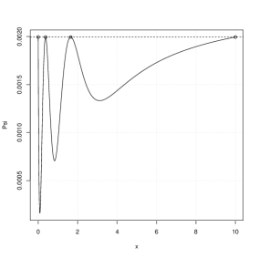
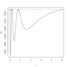
(1)                                          (2)                                          (3)

Figure 1: The function on the left hand side of inequality (2.5) in the equivalence Theorem 2.1 for the numerically calculated Bayesian KL-optimal discriminating designs. The competing regression models are given in (4.4).

The Bayesian KL-optimal discriminating designs for log-normal distributed responses are displayed in Table 2 for the different specifications of the mean and variance in (4.3). In Figure 1 we show the function on the left hand side of inequality (2.5) in the equivalence Theorem 2.1. Comparing the computational times in Table 2 we observe again that using quadratic programming in Step 2 of Algorithm 3.2 is substantially faster than the gradient method.
It might be of interest to compare the Bayesian optimal discriminating designs for the various log-normal distributed responses with the design for normal distributed responses determined in Dette et al., (2015). This design is supported at the five(!) points $0.000$, $0.452$, $1.747$, $4.951$ and $10.000$ with masses $0.207$, $0.396$, $0.292$, $0.003$ and $0.102$, respectively. The efficiencies

$$\mathrm{Eff}_{KL_{P}}^{(j)}(\xi_{(i)}^{*})=\frac{KL_{P}^{(j)}(\xi_{(i)}^{*})}{\sup_{\eta}KL_{P}^{(j)}(\eta)}.$$

under misspecification of the distribution of the response are depicted in Table 3. For example, the efficiency of the design $\xi^{*}_{(0)}$ calculated under the assumption homoscedastic normal distributed responses in the model with log-normal distributed responses in (4.3)(2) is given by $95.3\%$. We observe that the Bayesian optimal discriminating designs calculated for normal distributed responses are rather robust and have good efficiencies for the log-normal distribution.

(4.3)	design	AF	grad	quad
(1)	$\begin{matrix}0&0.406&1.706&10\\ 0.186&0.418&0.289&0.107\end{matrix}$	298.37	44.36	3.7
(2)	$\begin{matrix}0&0.374&1.650&10\\ 0.189&0.397&0.311&0.103\end{matrix}$	390.44	7.39	2.39
(3)	$\begin{matrix}0&0.356&1.604&10\\ 0.186&0.394&0.313&0.107\end{matrix}$	570.45	39.19	4.42

Table 2: Bayesian KL-optimal discriminating designs for the models in (4.4). The responses are log-normal distributed with different specifications of the mean and variance - see (4.3). The prior distribution is defined by (4.5) and (4.6). Column three and four show the computation time of the new Algorithm 3.2 proposed in this paper with a gradient (grad) and quadratic programming method (quad) in Step 2.

	(0)	(1)	(2)	(3)
(0)	1	0.978	0.953	0.908
(1)	0.981	1	0.988	0.966
(2)	0.951	0.987	1	0.992
(3)	0.923	0.970	0.996	1

Table 3: Efficiencies of Bayesian KL-optimal discriminating designs for the models in (4.4) under different distributional assumptions for the responses. (0): homoscedastic normal distribution; (1) - (3): log-normal distribution with different specifications of the mean and variance - see (4.3).

(4.9)	design	AF	grad	quad
(1)	$\begin{matrix}0.759&67.32&248.6&500\\ 0.419&0.156&0.233&0.192\end{matrix}$	1674.14	679.52	48.91
(2)	$\begin{matrix}0&58.9&220.6&500\\ 0.200&0.354&0.247&0.199\end{matrix}$	-	255.03	33.42
(3)	$\begin{matrix}0&33.12&78.0&161.6&215.7&500\\ 0.279&0.092&0.225&0.003&0.224&0.177\end{matrix}$	2382.64	631.53	82.33

Table 4: Bayesian KL-optimal discriminating designs for the competing dose response models in (4.7). The responses are log-normal distributed with different specifications of the mean and variance - see (4.9). The prior distribution is a uniform distribution on $81$ points as specified in (4.8). Column three, four and five show the computation time of the exchange type algorithm (AF), the new Algorithm 3.2 proposed in this paper with a gradient (grad) and quadratic programming method (quad) in Step 2.

Example 4.3

Our final example refers to the construction of Bayesian KL-optimal discriminating designs for several dose response curves, which have been recently proposed by Pinheiro et al., (2006) for modeling the dose response relationship of a Phase II clinical trial, that is

$$\eta_{1}(x,\theta_{1})=\theta_{1,1}+\theta_{1,2}x;$$

(4.7) $$\eta_{2}(x,\theta_{2})=\theta_{2,1}+\theta_{2,2}x(\theta_{2,3}-x);$$

$$\eta_{3}(x,\theta_{3})=\theta_{3,1}+\theta_{3,2}x/(\theta_{3,3}+x);$$

$$\eta_{4}(x,\theta_{4})=\theta_{4,1}+\theta_{4,2}/(1+\exp(\theta_{4,3}-x)/\theta_{4,4});$$

where the designs space (dose range) is given by the interval $\mathcal{X}=[0,500]$. In this reference some prior information regarding the parameters for the models is also provided., that is

$$\overline{\theta}_{1}=(60,0.56),\;\overline{\theta}_{2}=(60,7/2250,600),\;\overline{\theta}_{3}=(60,294,25),\;\ \overline{\theta}_{4}=(49.62,290.51,150,45.51).$$

Dette et al., (2015) determined Bayesian KL-optimal discriminating designs for these models under the assumption of normal distributed responses, where they used $p_{i,j}=1/6$, $(1\leq j<i\leq 4)$ and they assumed that there exist only uncertainty for the parameter $\theta_{4}$. We will now consider similar problems for log-normal distributed responses, where the prior distribution is a uniform distribution at $81$ points in $\mathbb{R}^{4}$, that is

(4.8) $$(49.62+c_{1},290.51+c_{2},150+c_{3},45.51+c_{4})$$

with $c_{1},c_{2},c_{3},c_{4}\in\{-20,0,45\}$. Note that we cannot use the prior distribution considered in Dette et al., (2015) because this would yield a negative mean $\eta_{i}(x,\theta_{i})$. The resulting Bayesian optimality criterion (2.8) consist of $246$ model comparisons and Bayesain KL–optimal discriminating designs are depicted in Table 4 for the cases

(4.9) $$\begin{array}[]{ll}(1)&v^{2}_{1}(x,\theta_{1})=1~{},~{}i=1,2,3,4;\\ (2)&\sigma^{2}_{i}(x,\theta_{i})=1~{},~{}i=1,2,3,4;\\ (3)&v_{i}^{2}(x,\theta_{i})=\exp(\eta_{i}(x,\theta_{i})/100)~{},~{}i=1,2,3,4.\end{array}$$

All calculated designs have at least efficiency $99.9\%$ and the corresponding plots of the equivalence Theorem 2.1 are shown in Figure 2. In the models specified by (4.7) all new algorithms were able to find the Bayesian KL-optimal discriminating design, where the exchange type algorithm failed in the case (4.9)(2). Moreover, in the other cases the new methods are substantially faster than the exchange type method. For example, the gradient method yields only $25\%-30\%$ of the computational time, while the quadratic programming approach is about $30-35$ times faster.

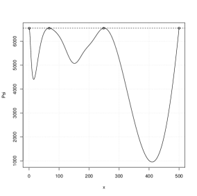
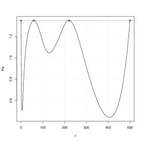
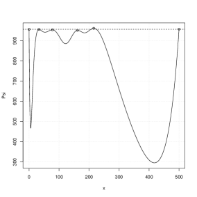
(1)                                          (2)                                          (3)

Figure 2: The function on the left hand side of inequality (2.5) in the equivalence Theorem 2.1 for the numerically calculated Bayesian KL-optimal discriminating designs. The competing regression models are given in (4.7) and the scenarios for log-normal distribution specified in (4.9).

5 Appendix: Proof of Lemma 3.3

By the construction of the function $\overline{g}$ we have $\overline{g}(\omega)\leq g(\omega)$ for all $\omega\in\Delta$. Let $\omega^{*}\in\operatorname*{arg\,max}_{\omega\in\Delta}g(\omega)$ and define the function

$$\Psi_{i,j}(\theta_{i,j},\omega)=\sum_{k=1}^{n}\omega_{k}\int\log\left\{\frac{f_{i}(x_{k},y,\overline{\theta}_{i})}{f_{j}(x_{k},y,{\theta}_{i,j})}\right\}f_{i}(x_{k},y,\overline{\theta}_{i})d\mu(dy)$$

If $\widehat{\theta}_{i,j}=\operatorname*{argmin}_{\theta_{i,j}\in\Theta_{j}}\Psi_{i,j}(\theta_{i,j},\omega^{*})$ is the miminizer of $\Psi_{i,j}$ it follows from Assumption 2.2 that

$$\frac{\partial}{\partial\theta_{i,j}}\Psi_{i,j}(\theta_{i,j},\omega^{*})\Big{|}_{\theta_{i,j}=\widehat{\theta}_{i,j}}=\mathbf{R}_{i,j}(\widehat{\theta}_{i,j})\omega^{*}=0,$$

and we obtain

$$\widehat{\alpha}_{i,j}=\left(\int\mathbf{J}_{i,j}^{T}(y)\Omega\mathbf{J}_{i,j}(y)dy\right)^{-1}\mathbf{R}_{i,j}^{T}(\widehat{\theta}_{i,j})\omega^{*}=0$$

Inserting this value in (3.2) gives $\overline{g}(\omega^{*})={g}(\omega^{*})$, i.e. $\max_{\omega\in\Delta}\overline{g}(\omega)=\max_{\omega\in\Delta}g(\omega)$. Now let $\omega^{*}=\operatorname*{arg\,max}_{\omega\in\Delta}\overline{g}(\omega)$. From the above equality it follows that $\widehat{\alpha}_{i,j}=0$ and therefore $\mathbf{R}_{i,j}(\widehat{\theta}_{i,j})\omega^{*}=0$, that is $\omega^{*}=\operatorname*{arg\,max}g(\omega)$. $\Box$

Acknowledgements. Parts of this work were done during a visit of the second author at the Department of Mathematics, Ruhr-Universität Bochum, Germany. The authors would like to thank M. Stein who typed this manuscript with considerable technical expertise. The work of H. Dette and V. Melas was supported by the Deutsche Forschungsgemeinschaft (SFB 823: Statistik nichtlinearer dynamischer Prozesse, Teilprojekt C2). The research of H. Dette reported in this publication was also partially supported by the National Institute of General Medical Sciences of the National Institutes of Health under Award Number R01GM107639. The content is solely the responsibility of the authors and does not necessarily represent the official views of the National Institutes of Health. The work of V. Melas and R. Guchenko was also partially supported by by St. Petersburg State University (project ”Actual problems of design and analysis for regression models”, 6.38.435.2015).

References

- Atkinson et al., (2007) Atkinson, A., Donev, A., and Tobias, R. (2007). Optimum Experimental Designs, with SAS (Oxford Statistical Science Series). Oxford University Press, USA, 2nd edition.
- (2) Atkinson, A. C. and Fedorov, V. V. (1975a). The designs of experiments for discriminating between two rival models. Biometrika, 62:57–70.
- (3) Atkinson, A. C. and Fedorov, V. V. (1975b). Optimal design: Experiments for discriminating between several models. Biometrika, 62:289–303.
- Biedermann et al., (2006) Biedermann, S., Dette, H., and Pepelyshev, A. (2006). Some robust design strategies for percentile estimation in binary response models. Canadian Journal of Statistics, 34:603–622.
- Braess and Dette, (2013) Braess, D. and Dette, H. (2013). Optimal discriminating designs for several competing regression models. Annals of Statistics, 41(2):897–922.
- Chernoff, (1953) Chernoff, H. (1953). Locally optimal designs for estimating parameters. Annals of Mathematical Statistics, 24:586–602.
- Crawley, (2002) Crawley, M. J. (2002). Statistical Computing: an Introduction to Data Analysis using S-Plus. Wiley, New York.
- Dette, (1990) Dette, H. (1990). A generalization of - and -optimal designs in polynomial regression. Annals of Statistics, 18:1784–1805.
- Dette et al., (2008) Dette, H., Bretz, F., Pepelyshev, A., and Pinheiro, J. (2008). Optimal designs for dose-finding studies. Journal of the American Statistical Association, 104(483):1225–1237.
- Dette and Haller, (1998) Dette, H. and Haller, G. (1998). Optimal designs for the identification of the order of a Fourier regression. Annals of Statistics, 26:1496–1521.
- Dette et al., (2015) Dette, H., Melas, V. B., and Guchenko, R. (2015). Bayesian -optimal discriminating designs. Annals of Statistics, to appear,.
- Dette et al., (2012) Dette, H., Melas, V. B., and Shpilev, P. (2012). T-optimal designs for discrimination between two polynomial models. Annals of Statistics, 40(1):188–205.
- Kiefer, (1974) Kiefer, J. (1974). General equivalence theory for optimum designs (approximate theory). Annals of Statistics, 2(5):849–879.
- Läuter, (1974) Läuter, E. (1974). Experimental design in a class of models. Math. Operationsforsch. Statist., 5(4 & 5):379–398.
- Lindsey et al., (2001) Lindsey, J. K., Jones, B., and Jarvis, P. (2001). Some statistical issues in modelling pharmacokinetic data. Statistics in Medicine, 20:2775–2783.