Improved ZZ A Posteriori Error Estimators for Diffusion Problems:
Conforming Linear Elements

Abstract

In [8], we introduced and analyzed an improved Zienkiewicz-Zhu (ZZ) estimator for the conforming linear finite element approximation to elliptic interface problems. The estimator is based on the piecewise “constant” flux recovery in the $H({\rm div};\Omega)$ conforming finite element space. This paper extends the results of [8] to diffusion problems with full diffusion tensor and to the flux recovery both in piecewise constant and piecewise linear $H({\rm div})$ space.

1 Introduction

A posteriori error estimation for finite element methods has been extensively studied for the past four decades (see, e.g., books by Ainsworth and Oden [1], Babuška and Strouboulis [3], and Verfürth [25] and references therein). Due to easy implementation, generality, and ability to produce quite accurate estimation, the Zienkiewicz-Zhu (ZZ) recovery-based error estimator [31] has been widely adapted in engineering practice and has been the subject of mathematical study (e.g., [4, 5, 10, 12, 13, 16, 19, 23, 24, 26, 28, 29, 30, 32]). By first recovering a gradient (flux) in the conforming $C^{0}$ linear vector finite element space from the numerical gradient (flux), the ZZ estimator is defined as the $L^{2}$ norm of the difference between the recovered and the numerical gradients/fluxes.

Despite popularity of the ZZ estimator, it is also well known (see, e.g., [20, 21]) that adaptive mesh refinement (AMR) algorithms using the ZZ estimator are not efficient to reduce global error for non-smooth problems, e.g., interface problems. This is because they over-refine regions where there are only small errors. By exploring the mathematical structure of the underlying problem and the characteristics of finite element approximations, in [8, 9] we identified that this failure of the ZZ estimator is caused by using a continuous function (the recovered gradient (flux)) to approximate a discontinuous one (the true gradient (flux)) in the recovery procedure. Therefore, to fix this structural failure, we should recover the gradient (flux) in proper finite element spaces. More specifically, for the conforming linear finite element approximation to the interface problem we recovered the flux in the $H({\rm div};\Omega)$ conforming finite element space. It was shown in [8] that the resulting implicit and explicit error estimators are not only reliable but also efficient. Moreover, the estimators are robust with respect to the jump of the coefficients.

In [8], the implicit error estimator requires solution of a global $L^{2}$ minimization problem, and the explicit error estimator uses a simple edge average. This averaging approach of the explicit estimator is limited to the Raviart-Thomas ($RT$) [7] element of the lowest order, i.e., the piecewise “constant” vector. In this paper, we introduce a general approach of constructing explicit flux recoveries using either the piecewise “constant” vector or the piecewise linear vector (the Brezzi-Douglas-Marini (BDM) [7] element of the lowest order) for the diffusion problem with the full diffusion coefficient tensor. With the recovered fluxes, the improved ZZ estimators are defined as a weighted $L^{2}$ norm of the difference between the recovered and the numerical fluxes. These estimators are theoretically shown to be locally efficient and globally reliable. Moreover, when the diffusion coefficient is piecewise constant scalar and its distribution is locally quasi-monotone, these estimators are robust with respect to the size of jumps. For a benchmark test problem, whose coefficient is not locally quasi-monotone, numerical results also show the robustness of the estimators.

The paper is organized as follows. Section 2 describes the diffusion problem, variational form, and conforming finite element approximation. Section 3 describes the a posteriori error estimators of the ZZ type and two counter-examples. Two explicit flux recoveries and their corresponding improved ZZ estimators are introduced in section 4. Efficiency and reliability of those estimators are established in section 5. Section 6 is devoted to explicit formulas of the recovered fluxes, the indicators, and the estimators. Finally, section 7 presents numerical results on the Kellogg’s benchmark test problem.

2 Finite Element Approximation to Diffusion Problem

Let $\Omega$ be a bounded polygonal domain in $\Re^{d}$ with $d=2$ or $3$, with boundary $\partial\Omega=\overline{\Gamma}_{{}_{D}}\cup\overline{\Gamma}_{{}_{N}}$, $\Gamma_{{}_{D}}\cap\Gamma_{{}_{N}}=\emptyset$, and $\mbox{meas}_{d-1}\,(\Gamma_{{}_{D}})\not=0$, and let ${\bf n}$ be the outward unit vector normal to the boundary. Consider diffusion equation

$$-\nabla\cdot(A(x)\nabla u)=f\quad\mbox{in}\,\,\Omega$$ (2.1)

with boundary conditions

$$-A\nabla u\cdot{\bf n}=g_{{}_{N}}\quad\mbox{on}\,\,\Gamma_{{}_{N}}\quad\mbox{and}\quad u=g_{{}_{D}}\quad\mbox{on}\,\,\Gamma_{{}_{D}},$$ (2.2)

where the $\nabla\cdot$ and $\nabla$ are the divergence and gradient operators, respectively, and $f\in L^{2}(\Omega)$. In this paper, we consider only simplicial elements. Let ${\cal T}=\{K\}$ be a regular triangulation of the domain $\Omega$, and denote by $h_{{}_{K}}$ the diameter of the element $K$. For simplicity of presentation, assume that $g_{{}_{D}}$ and $g_{{}_{N}}$ are piecewise affine functions and constants, respectively, and that $A$ is a piecewise constant matrix that is symmetric, positive definite.

Let

$$H^{1}_{{}_{g,D}}(\Omega)=\{v\in H^{1}(\Omega)\,:\,v=g_{{}_{D}}\mbox{ on }\Gamma_{{}_{D}}\}\quad\mbox{and}\quad H^{1}_{{}_{D}}(\Omega)=H^{1}_{{}_{0,D}}(\Omega).$$

Then the corresponding variational problem is to find $u\in H^{1}_{{}_{g,D}}(\Omega)$ such that

$$a(u,\,v)\equiv(A\nabla u,\nabla v)=(f,v)-(g_{{}_{N}},v)_{\Gamma_{{}_{N}}}\equiv f(v)\quad\forall\;v\in H^{1}_{{}_{D}}(\Omega),$$ (2.3)

where $(\cdot,\cdot)_{\omega}$ is the $L^{2}$ inner product on the domain $\omega$. The subscript $\omega$ is omitted when $\omega=\Omega$.

For each $K\in{\cal T}$, let $P_{k}(K)$ be the space of polynomials of degree less than or equal to $k$. Denote the linear conforming finite element space [15] associated with the triangulation ${\cal T}$ by

$${\cal S}=\{v\in H^{1}(\Omega)\,:\,v|_{K}\in P_{1}(K)\quad\forall\,\,K\in{\cal T}\}.$$

Let

$${\cal S}_{g,{{}_{D}}}=\{v\in{\cal S}:\,v=g_{{}_{D}}\,\,\mbox{on}\,\,\Gamma_{{}_{D}}\}\quad\mbox{and}\quad{\cal S}_{{{}_{D}}}={\cal S}_{{}_{0,D}}$$

Then the conforming finite element approximation is to seek $u_{{}_{\cal T}}\in{\cal S}_{g,{{}_{D}}}$ such that

$$(A\nabla u_{{}_{\cal T}},\,\nabla v) = f(v)\qquad\,\forall\,v\in{\cal S}_{{{}_{D}}}.$$ (2.4)

3 ZZ Error Estimator and Counter Examples

Let $\tilde{u}_{{}_{\cal T}}\in{\cal S}_{g,{{}_{D}}}$ be an approximation to the finite element solution $u_{{}_{\cal T}}\in{\cal S}_{g,{{}_{D}}}$ of (2.4). Denote the numerical gradient and the numerical flux by

$$\tilde{\mbox{\boldmath$\rho$}}_{{}_{\cal T}}=\nabla\tilde{u}_{{}_{\cal T}}\quad\mbox{and}\quad\tilde{\mbox{\boldmath$\sigma$}}_{{}_{\cal T}}=-A\,\nabla\tilde{u}_{{}_{\cal T}},$$ (3.1)

respectively, which are piecewise constant vectors in $\Re^{d}$ with respect to the triangulation ${\cal T}$. It is common in engineering practice to smooth the piecewise constant gradient or flux in a post-process so that they are continuous. More precisely, denote by ${\cal N}$ the set of all vertices of the triangulation ${\cal T}$. For each vertex $z\in{\cal N}$, denote by $\omega_{z}$ the union of elements having $z$ as the common vertex. The recovered (smoothed) gradient or flux are defined as follows: for $\mbox{\boldmath$\tau$}=\tilde{\mbox{\boldmath$\rho$}}_{{}_{\cal T}}$ or $\tilde{\mbox{\boldmath$\sigma$}}_{{}_{\cal T}}$

$$G(\mbox{\boldmath$\tau$})\in{\cal S}^{d}\subset C^{0}(\Omega)^{d}\quad\mbox{with nodal values}\quad G(\mbox{\boldmath$\tau$})(z)=\displaystyle\frac{1}{|\omega_{z}|}\int_{\omega_{z}}\mbox{\boldmath$\tau$}\,dx\quad\forall\,\,z\in{\cal N},$$ (3.2)

where $|\omega_{z}|=\mbox{meas}_{d}(\omega_{z})$. There are many post-processing, recovery techniques (see survey article [29] by Zhang and references therein). With the recovered gradient (flux), the ZZ error indicator and estimator are defined as follows:

$$\xi_{{}_{ZZ,K}}=\|G(\mbox{\boldmath$\tau$})-\mbox{\boldmath$\tau$}\|_{0,K}\quad\forall\,\,K\in{\cal T}\quad\mbox{and}\quad\xi_{{}_{ZZ}}=\|G(\mbox{\boldmath$\tau$})-\mbox{\boldmath$\tau$}\|_{0,\Omega}$$

for $\mbox{\boldmath$\tau$}=\tilde{\mbox{\boldmath$\rho$}}_{{}_{\cal T}}$ or $\tilde{\mbox{\boldmath$\sigma$}}_{{}_{\cal T}}$, respectively.

Despite many attractive features of the ZZ error estimator, it is well known (see Figures in section 7 that adaptive mesh refinement (AMR) algorithms using the above ZZ estimator are not efficient to reduce global error for interface problems. In this section, we demonstrate this failure of the ZZ estimator by two counter-examples for which the finite element solution is exact while the ZZ indicators along interface could be arbitrarily large.

The first example is a one-dimensional interface problem defined on the domain $\Omega=(0,\,1)$ with the Dirichlet boundary condition:

$$u(0)=0\quad\mbox{and}\quad u(1)=(k+1)/2$$

for an arbitrary constant $k>1$ and with piecewise constant diffusion coefficient

$$A=1\quad\mbox{in }\,(0,\,1/2)\quad\mbox{and}\quad A=k>0\quad\mbox{in }\,(1/2,\,1).$$

The exact solution and its derivative of this example are piecewise linear and piecewise constant functions, respectively, depicted in Figures 1 and 2 and given by

$$u=\left\{\begin{array}[]{ll}k\,x&x\in(0,\,1/2\,],\\[5.69054pt] x+\displaystyle\frac{k-1}{2}&x\in(1/2,\,1),\end{array}\right.\quad\mbox{and}\quad u^{\prime}=\left\{\begin{array}[]{ll}k&x\in(0,\,1/2),\\[5.69054pt] 1&x\in(1/2,\,1).\end{array}\right.$$

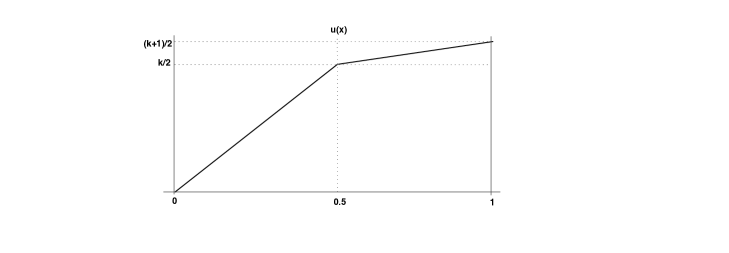
Figure 1: solution $u=u_{{}_{\cal T}}$

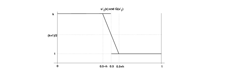
Figure 2: $u_{{}_{\cal T}}^{\prime}(x)$ and $G(u_{{}_{\cal T}}^{\prime})$

For any triangulation ${\cal T}$ with $x=1/2$ as one of its vertices, the conforming linear finite element approximation is identical to the exact solution: $u_{{}_{\cal T}}=u$, and hence the true error equals to zero. Without loss of generality, assume that the size of two interface elements is $h$. Then the recovered gradient is depicted in Figure 2 and its value at $x=1/2$ is $(k+1)/2$. A simple calculation yields the ZZ error indicator:

$$\xi_{{}_{Z\!Z,K}}=\|G(u_{{}_{\cal T}}^{\prime})-u_{{}_{\cal T}}^{\prime}\|_{0,K}=\left\{\begin{array}[]{lll}\displaystyle\frac{1}{2\sqrt{3}}(k-1)\,h^{1/2},&x\in(1/2-h,\,1/2),\\[11.38109pt] \displaystyle\frac{1}{2\sqrt{3}}(k-1)\,h^{1/2},&x\in(1/2,\,1/2+h),\\[11.38109pt] 0,&\mbox{otherwise}.\end{array}\right.$$

Hence, no matter how small the mesh size $h$ is, the ZZ indicators at two interface elements could be arbitrarily large.

For this simple one-dimensional example, to overcome the inefficiency of the estimator, one may use the ZZ estimator based on the flux. However, this idea could not be extended to two or three dimensions. To see this, consider the second example defined on the domain $\Omega=(-1,\,1)^{2}$ with scalar piecewise constant diffusion coefficient

$$A=kI\quad\mbox{for }\,y>0\quad\mbox{and}\quad A=I\quad\mbox{for }\,y<0,$$

where $k>1$ is an arbitrary constant. Choose proper Dirichlet boundary data such that the exact solution of (2.1) is piecewise linear function given by

$$u=\left\{\!\!\begin{array}[]{llll}x+y&\,\,\mbox{if}&y>0,\\[5.69054pt] x+k\,y&\,\,\mbox{if}&y<0.\end{array}\right.$$

The conforming linear finite element approximation on any triangulation aligned with the interface $y=0$ is identical to the exact solution, and hence the true error vanishes. Since the exact gradient and flux

$$\nabla u=\left\{\begin{array}[]{ll}(1,\,1)^{t},&\mbox{for }\,y>0,\\[5.69054pt] (1,\,k)^{t},&\mbox{for }\,y<0\end{array}\right.\quad\mbox{and}\quad\mbox{\boldmath$\sigma$}=-A\nabla u=\left\{\begin{array}[]{ll}(k,\,k)^{t},\!&\mbox{for }\,y>0,\\[5.69054pt] (1,\,k)^{t},\!&\mbox{for }\,y<0\end{array}\right.$$

are not continuously across the interface, similar calculation to the first example yields that the ZZ error indicators on the interface elements based on continuous gradient or flux recovery could be arbitrarily large no matter how small the mesh sizes of the interface elements are.

4 Improved ZZ Estimators

The second example of the previous section shows that the gradient and the flux of the exact solution of (2.1) are not continuously across interfaces. This means that inefficiency of the ZZ estimator is caused by using continuous functions (the recovered gradient or flux) to approximate discontinuous functions (the true gradient or flux). In this section, we introduce improved ZZ estimator that is efficient.

To this end, let

$$H({\rm div};\Omega)=\{\mbox{\boldmath$\tau$}\in L^{2}(\Omega)^{d}\,:\,\nabla\cdot\mbox{\boldmath$\tau$}\in L^{2}(\Omega)\}\not\subset H^{1}(\Omega)^{d}$$

with the norm $\|\mbox{\boldmath$\tau$}\|_{H({\rm div};\,\Omega)}=\left(\|\mbox{\boldmath$\tau$}\|^{2}_{0,\Omega}+\|\nabla\cdot\mbox{\boldmath$\tau$}\|^{2}_{0,\Omega}\right)^{1/2}$ and let

$$H_{g,_{N}}({\rm div};\Omega)\!=\{\mbox{\boldmath$\tau$}\in H({\rm div};\Omega)\,:\,\mbox{\boldmath$\tau$}\cdot{\bf n}|_{\Gamma_{{}_{N}}}=g_{{}_{N}}\}.$$

Denote the $H({\rm div};\,\Omega)$ conforming Raviart-Thomas ($RT$) and Brezzi-Douglas-Marini ($B\!D\!M$) spaces [7] of the lowest order by

$$RT=\{\mbox{\boldmath$\tau$}\in H({\rm div};\,\Omega)\,:\,\mbox{\boldmath$\tau$}|_{K}\in RT(K)\,\,\,\,\forall\,K\in{\cal T}\}$$

and $$B\!D\!M=\{\mbox{\boldmath$\tau$}\in H({\rm div};\,\Omega)\,:\,\mbox{\boldmath$\tau$}|_{K}\in B\!D\!M(K)\,\,\,\,\forall\,\,K\in{\cal T}\},$$

respectively, where $RT(K)=P_{0}(K)^{d}+(x_{1},\,...,\,x_{d})^{t}\,P_{0}(K)$ and $B\!D\!M(K)=P_{1}(K)^{d}$. Let

$$RT_{g,N}=RT\cap H_{g,N}({\rm div};\Omega)\quad\mbox{and}\quad B\!D\!M_{g,N}=B\!D\!M\cap H_{g,N}({\rm div};\Omega).$$

Let $u\in H^{1}(\Omega)$ be the exact solution of (2.1), it is well known that the tangential components of the gradient and the normal component of the flux are continuous. Mathematically, we have

$$``u\in H^{1}(\Omega)\Longrightarrow\nabla u\in H(\mbox{curl};\Omega)"\quad\mbox{and}\quad\mbox{\boldmath$\sigma$}=-A\nabla u\in H({\rm div};\Omega),$$

where $H(\mbox{curl};\Omega)\not\subset H^{1}(\Omega)^{d}$ is the collection of vector-valued functions that are square integrable and whose curl are also square integrable. This suggests that proper finite element spaces for recovering the gradient and the flux are the respective $H(\mbox{curl};\Omega)$ and $H({\rm div};\Omega)$ conforming finite element spaces.

For the conforming finite element approximation, the numerical gradient $\tilde{\mbox{\boldmath$\rho$}}_{{}_{\cal T}}$ is already in $H(\mbox{curl};\Omega)$ and, hence, the resulting improved ZZ estimator based on the gradient recovery is identical to zero. Since the numerical flux $\tilde{\mbox{\boldmath$\sigma$}}_{{}_{\cal T}}$ is not in $H_{g,N}({\rm div};\Omega)$, the improved ZZ estimators introduced in [8] are based on either explicit or implicit flux recoveries in $RT_{g,N}$ and $B\!D\!M_{g,N}$. The explicit recovery is limited to the scalar diffusion coefficient and the $RT$ element. The implicit recovery requires to solve the following global $L^{2}$ minimization problem: find $\bar{\mbox{\boldmath$\sigma$}}_{{}_{\cal T}}\in{\cal V}$ such that

$$\|A^{-1/2}(\bar{\mbox{\boldmath$\sigma$}}_{{}_{\cal T}}-\tilde{\mbox{\boldmath$\sigma$}}_{{}_{\cal T}})\|_{0,\Omega}=\min_{\mbox{\boldmath$\tau$}\in{\cal V}}\,\,\|A^{-1/2}(\mbox{\boldmath$\tau$}-\tilde{\mbox{\boldmath$\sigma$}}_{{}_{\cal T}})\|_{0,\Omega},$$ (4.1)

where ${\cal V}=RT_{g,N}$ or $B\!D\!M_{g,N}$. With the recovered flux $\bar{\mbox{\boldmath$\sigma$}}_{{}_{\cal T}}\in{\cal V}$, the improved ZZ estimator introduced in [8] is given by

$$\xi\,(\bar{\mbox{\boldmath$\sigma$}}_{{}_{\cal T}})=\|A^{-1/2}(\bar{\mbox{\boldmath$\sigma$}}_{{}_{\cal T}}-\tilde{\mbox{\boldmath$\sigma$}}_{{}_{\cal T}})\|_{0,\Omega}.$$ (4.2)

Even though the solution of (4.1) may be computed efficiently by a simple iterative solver, in the remainder of this section, we derive two new explicit and efficient flux recoveries applicable to the problem with the full diffusion tensor based on the respective $RT$ and $B\!D\!M$ elements of the lowest order.

Here, we introduce some notations. Denote the set of all edges (faces) of the triangulation by ${\cal E}:={\cal E}_{{}_{I}}\cup{\cal E}_{{}_{D}}\cup{\cal E}_{{}_{N}},$ where ${\cal E}_{{}_{I}}$ is the set of all interior element edges (faces), and ${\cal E}_{{}_{D}}$ and ${\cal E}_{{}_{N}}$ are the sets of all boundary edges (faces) belonging to the respective $\Gamma_{{}_{D}}$ and $\Gamma_{{}_{N}}$. For each $F\in{\cal E}$, denote by ${\bf n}_{{}_{F}}$ the unit vector normal to $F$. For each $F\in{\cal E}_{{}_{I}}$, let $K_{{}_{F}}^{-}$ and $K_{{}_{F}}^{+}$ be two elements sharing the common edge (face) $F$ such that the unit outward normal vector of $K_{{}_{F}}^{-}$ coincides with ${\bf n}_{{}_{F}}$; and let ${\bf x}_{F}^{-}$ and ${\bf x}_{F}^{+}$ be the vertex of $K_{F}^{+}$ and $K_{F}^{-}$ opposite to $F$, respectively. When $F\in{\cal E}_{{}_{D}}\cup{\cal E}_{{}_{N}}$, ${\bf n}_{{}_{F}}$ is the unit outward vector normal to $\partial\Omega$ and denote by $K_{{}_{F}}^{-}$ the element having the edge (face) $F$ and by ${\bf x}_{F}^{-}$ the vertex in $K_{F}^{-}$ opposite to $F$.

Let $\delta$ be the Kronecker delta function. For each $F\in{\cal E}$, denote by $\mbox{\boldmath$\phi$}_{{}_{F}}$ the global nodal basis function of $RT$ associated with $F$, i.e.,

$$\int_{F^{\prime}}\left(\mbox{\boldmath$\phi$}_{{}_{F}}\cdot{\bf n}_{{{}_{F}}^{\prime}}\right)\,ds=\delta_{{}_{FF^{\prime}}},\quad\forall\,\,F^{\prime}\in{\cal E};$$ (4.3)

denote by $\mbox{\boldmath$\psi$}_{{}_{1,F}},\,...,\,\mbox{\boldmath$\psi$}_{{}_{d,F}}$ global basis functions of $B\!D\!M$ satisfying

$$\mbox{\boldmath$\psi$}_{{}_{1,F}}+\cdots+\mbox{\boldmath$\psi$}_{{}_{d,F}}=\mbox{\boldmath$\phi$}_{{}_{F}},\quad\forall\,\,F\in{\cal E};$$ (4.4)

and let

$$RT_{{}_{F}}=\mbox{span}\{\mbox{\boldmath$\phi$}_{{}_{F}}\}\quad\mbox{and}\quad B\!D\!M_{{}_{F}}=\mbox{span}\{\mbox{\boldmath$\psi$}_{{}_{1,F}},\,...,\,\mbox{\boldmath$\psi$}_{{}_{d,F}}\}.$$

Since ${\bf g}_{{}_{N}}$ is piecewise constant, for any $\mbox{\boldmath$\tau$}\in RT_{g,N}$ or $B\!D\!M_{g,N}$, we have that

$$\mbox{\boldmath$\tau$}=\sum_{F\in\,{\cal E}_{{}_{I}}\cup\,{\cal E}_{{}_{D}}}\mbox{\boldmath$\tau$}_{{}_{F}}+\sum_{F\in\,{\cal E}_{{}_{N}}}g_{{}_{N,F}}|F|\,\mbox{\boldmath$\phi$}_{{}_{F}}\quad\mbox{ with }\,\mbox{\boldmath$\tau$}_{{}_{F}}\in RT_{{}_{F}}\,\mbox{ or }\,B\!D\!M_{{}_{F}},$$ (4.5)

where $g_{{}_{N,F}}=g_{{}_{N}}|_{{}_{F}}$ and $|F|=\mbox{meas}_{d-1}\,(F)$.

For any $K\in{\cal T}$, restriction of the numerical flux $\tilde{\mbox{\boldmath$\sigma$}}_{{}_{\cal T}}$ on $K$ is a constant vector and has the following representation in $RT(K)$ (see Lemma 4.4 of [8]):

$$\tilde{\mbox{\boldmath$\sigma$}}_{{}_{\cal T}}|_{{}_{K}}=\sum_{F\subset\partial K}\tilde{\sigma}_{{}_{F,K}}|F|\mbox{\boldmath$\phi$}_{{}_{F}},$$

where $\tilde{\sigma}_{{}_{F,K}}=\left(\tilde{\mbox{\boldmath$\sigma$}}_{{}_{\cal T}}|_{K}\cdot{\bf n}_{{}_{F}}\right)_{{}_{F}}$ is the normal component of $\tilde{\mbox{\boldmath$\sigma$}}_{{}_{\cal T}}|_{K}$ on $F$. On each interior edge (face) $F\in{\cal E}_{{}_{I}}$, the normal component of the numerical flux has two values

$$\tilde{\sigma}_{{{}_{F}}}^{-}=\tilde{\sigma}_{{}_{F,K^{-}_{{}_{F}}}}\quad\mbox{and}\quad\tilde{\sigma}_{{{}_{F}}}^{+}=\tilde{\sigma}_{{}_{F,K^{+}_{{}_{F}}}}.$$

Denote by $\mbox{\boldmath$\phi$}^{-}_{{{}_{F}}}$ and $\mbox{\boldmath$\phi$}^{+}_{{{}_{F}}}$ the restriction of $\mbox{\boldmath$\phi$}_{{{}_{F}}}$ on $K_{{}_{F}}^{-}$ and $K_{{}_{F}}^{+}$, respectively. Then the numerical flux also has the following edge (face) representation:

$$\tilde{\mbox{\boldmath$\sigma$}}_{{}_{\cal T}}=\sum_{F\in{\cal E}}\tilde{\mbox{\boldmath$\sigma$}}_{{{}_{F}}}\quad\mbox{with}\quad\tilde{\mbox{\boldmath$\sigma$}}_{{{}_{F}}}=\left\{\begin{array}[]{ll}\tilde{\sigma}_{{{}_{F}}}^{-}|F|\mbox{\boldmath$\phi$}^{-}_{{{}_{F}}}+\tilde{\sigma}_{{{}_{F}}}^{+}|F|\mbox{\boldmath$\phi$}^{+}_{{{}_{F}}},&\forall\,\,F\in{\cal E}_{{}_{I}},\\[5.69054pt] \tilde{\sigma}_{{{}_{F}}}^{-}|F|\mbox{\boldmath$\phi$}^{-}_{{{}_{F}}},&\forall\,\,F\in{\cal E}_{{}_{D}}\cup{\cal E}_{{}_{N}}.\end{array}\right.$$ (4.6)

For any $\mbox{\boldmath$\tau$}\in RT_{g,N}$ or $B\!D\!M_{g,N}$, (4.5) and (4.6) give

$$\mbox{\boldmath$\tau$}-\tilde{\mbox{\boldmath$\sigma$}}_{{}_{\cal T}}=\sum_{F\in{\cal E}_{{}_{I}}}\left(\mbox{\boldmath$\tau$}_{{}_{F}}-\tilde{\mbox{\boldmath$\sigma$}}_{{{}_{F}}}\right)+\sum_{F\in{\cal E}_{{}_{D}}}\left(\mbox{\boldmath$\tau$}_{{}_{F}}-\tilde{\sigma}_{{{}_{F}}}^{-}|F|\,\mbox{\boldmath$\phi$}_{{}_{F}}^{-}\right)+\sum_{F\in{\cal E}_{{}_{N}}}\left(g_{{}_{N,F}}-\tilde{\sigma}_{{{}_{F}}}^{-}\right)\,|F|\mbox{\boldmath$\phi$}_{{}_{F}}^{-},$$

which, together with the triangle inequality and the choice of $\mbox{\boldmath$\tau$}_{{}_{F}}=\tilde{\sigma}_{{{}_{F}}}^{-}\,|F|\mbox{\boldmath$\phi$}_{{}_{F}}^{-}$ for all $F\in{\cal E}_{{}_{D}}$, implies

$$\xi\,(\bar{\mbox{\boldmath$\sigma$}}_{{}_{\cal T}})=\min_{\mbox{\boldmath$\tau$}\in{\cal V}}\,\,\|A^{-1/2}\left(\mbox{\boldmath$\tau$}-\tilde{\mbox{\boldmath$\sigma$}}_{{}_{\cal T}}\right)\|_{0,\Omega}$$

$$\leq \sum_{F\in{\cal E}_{I}}\min_{\mbox{\boldmath$\tau$}_{{{}_{F}}}\in{\cal V}_{{{}_{F}}}}\,\,\|A^{-1/2}\left(\mbox{\boldmath$\tau$}_{{{}_{F}}}-\tilde{\mbox{\boldmath$\sigma$}}_{{{}_{F}}}\right)\|_{0,\omega_{{{}_{F}}}}+\sum_{F\in{\cal E}_{N}}\|A^{-1/2}\left(g_{{}_{N,F}}-\tilde{\sigma}_{{{}_{F}}}^{-}\right)\,|F|\mbox{\boldmath$\phi$}_{{}_{F}}^{-}\|_{0,K_{F}^{-}},$$ (4.7)

where $\omega_{{}_{F}}$ is the union of elements sharing the edge (face) $F$ for all $F\in{\cal E}$, ${\cal V}=RT_{g,N}$ or $B\!D\!M_{g,N}$ and ${\cal V}_{{}_{F}}=RT_{{}_{F}}$ or $B\!D\!M_{{}_{F}}$.

For each $F\in{\cal E}_{{}_{I}}$, let $\hat{\mbox{\boldmath$\sigma$}}_{{}_{F}}\in{\cal V}_{F}=RT_{{}_{F}}$ or $B\!D\!M_{{}_{F}}$ be the solution of the following local minimization problem:

$$\|A^{-1/2}\left(\hat{\mbox{\boldmath$\sigma$}}_{{}_{F}}-\tilde{\mbox{\boldmath$\sigma$}}_{{{}_{F}}}\right)\|_{0,\omega_{{{}_{F}}}}=\min_{\mbox{\boldmath$\tau$}\in{\cal V}_{{}_{F}}}\,\,\|A^{-1/2}\left(\mbox{\boldmath$\tau$}-\tilde{\mbox{\boldmath$\sigma$}}_{{{}_{F}}}\right)\|_{0,\omega_{{{}_{F}}}},$$ (4.8)

by (4.7), it is then natural to introduce the following edge (face) based estimator and indicators

$$\hat{\xi}=\sum_{F\in{\cal E}_{I}\,\cup\,{\cal E}_{N}}\xi_{{}_{F}}\quad\mbox{with}\quad\xi_{{}_{F}}=\left\{\begin{array}[]{ll}\|A^{-1/2}\left(\hat{\mbox{\boldmath$\sigma$}}_{{}_{F}}-\tilde{\mbox{\boldmath$\sigma$}}_{{{}_{F}}}\right)\|_{0,\omega_{{{}_{F}}}}&F\in{\cal E}_{I},\\[5.69054pt] \|A^{-1/2}\left(g_{{}_{N,F}}-\tilde{\sigma}_{{{}_{F}}}^{-}\right)\,|F|\mbox{\boldmath$\phi$}_{{}_{F}}^{-}\|_{0,K_{F}^{-}}&F\in{\cal E}_{N},\end{array}\right.$$ (4.9)

which satisfies

$$\xi\,(\bar{\mbox{\boldmath$\sigma$}}_{{}_{\cal T}})\leq\hat{\xi}.$$ (4.10)

To introduce the element based estimator, define the recovered flux $\hat{\mbox{\boldmath$\sigma$}}_{{}_{\cal T}}\in RT_{g,N}$ or $B\!D\!M_{g,N}$ as follows:

$$\hat{\mbox{\boldmath$\sigma$}}_{{}_{\cal T}}=\sum_{F\in{\cal E}_{{}_{I}}}\hat{\mbox{\boldmath$\sigma$}}_{{}_{F}}+\sum_{F\in{\cal E}_{{}_{D}}}\tilde{\sigma}_{{}_{F}}^{-}\,|F|\mbox{\boldmath$\phi$}_{{}_{F}}+\sum_{F\in{\cal E}_{{}_{N}}}g_{{}_{N,F}}\,|F|\mbox{\boldmath$\phi$}_{{}_{F}}.$$ (4.11)

Then the element based indicators and estimator are given by

$$\xi_{{}_{K}}=\|A^{-1/2}(\hat{\mbox{\boldmath$\sigma$}}_{{}_{\cal T}}-\tilde{\mbox{\boldmath$\sigma$}}_{{}_{\cal T}})\|_{0,K},\,\,\;\forall\,\,K\in{\cal T}\quad\mbox{and}\quad\xi=\|A^{-1/2}(\hat{\mbox{\boldmath$\sigma$}}_{{}_{\cal T}}-\tilde{\mbox{\boldmath$\sigma$}}_{{}_{\cal T}})\|_{0,\Omega}.$$ (4.12)

The minimization problem in (4.8) is equivalent to the following variational problem: find $\hat{\mbox{\boldmath$\sigma$}}_{{}_{F}}\in{\cal V}_{{{}_{F}}}$ such that

$$\left(A^{-1}\,\hat{\mbox{\boldmath$\sigma$}}_{{}_{F}},\,\mbox{\boldmath$\tau$}\right)_{\omega_{{{}_{F}}}}=\left(A^{-1}\,\tilde{\mbox{\boldmath$\sigma$}}_{{{}_{F}}},\,\mbox{\boldmath$\tau$}\right)_{\omega_{{{}_{F}}}}\quad\forall\,\,\mbox{\boldmath$\tau$}\in{\cal V}_{{}_{F}}.$$ (4.13)

The local problem in (4.13) has only one unknown if ${\cal V}_{{{}_{F}}}=RT_{{}_{F}}$ and $d$ unknowns if ${\cal V}_{{{}_{F}}}=B\!D\!M_{{}_{F}}$. The explicit formula of the solution $\hat{\mbox{\boldmath$\sigma$}}_{{}_{F}}$ will be given in section 6.

5 Efficiency and Reliability

This section establishes efficiency and reliability bounds of the indicators and estimators defined in (4.9) and (4.12), respectively, for the diffusion problem with the coefficient matrix $A$ being locally similar to the identity matrix.

To this end, for each $K\in{\cal T}$, denote by $\lambda_{\max,K}$ and $\lambda_{\min,K}$ the maximal and minimal eigenvalues of $A_{K}=A\big{|}_{K}$, respectively. Let

$$\lambda_{\max}=\max\limits_{K\,\in\,{\cal T}}\,\lambda_{\max,K}\quad\mbox{and}\quad\lambda_{\min}=\min\limits_{K\,\in\,{\cal T}}\,\lambda_{\min,K}.$$

Assume that each local matrix $A_{K}$ is similar to the identity matrix in the sense that its maximal and minimal eigenvalues are almost of the same size, i.e., there exists a moderate size constant $\kappa>0$ such that

$$\frac{\lambda_{\max,K}}{\lambda_{\min,K}}\,\leq\,\kappa,\quad\forall\;\,K\,\in{\cal T}.$$ (5.1)

Nevertheless, the ratio of the global maximal and minimal eigenvalues, $\lambda_{\max}\big{/}\lambda_{\min}$, could be very large. In order to show that the reliability constant is independent of the ratio, we assume that the distribution of $\lambda_{\min}(x)$ is quasi-monotone (see [22]).

Let $\Gamma_{{}_{I}}$ be the set of all interfaces of the diffusion coefficient that are assumed to be aligned with element interfaces, and denote by $f_{z}=\displaystyle\frac{1}{\mbox{meas}_{d}(\omega_{z})}\int_{\omega_{z}}f\,dx$ the average of $f$ over $\omega_{z}$. Let

$$\widehat{H}_{f}=\left\{\sum_{z\in{\cal N}\setminus(\overline{\Gamma}_{{}_{I}}\cup\overline{\Gamma}_{D})}\displaystyle\frac{\mbox{meas}_{d}(\omega_{z})}{\lambda_{\min,\omega_{z}}}\,\|f-f_{z}\|_{0,\omega_{z}}^{2}+\sum_{z\in{\cal N}\cap(\overline{\Gamma}_{{}_{I}}\cup\overline{\Gamma}_{D})}\sum_{K\subset\omega_{z}}\displaystyle\frac{h_{K}^{2}}{\lambda_{\min,K}}\,\|f\|_{0,K}^{2}\right\}^{1/2}.$$

Note that $A$ is a constant matrix in $\omega_{z}$ if $z\in{\cal N}\setminus(\overline{\Gamma}_{{}_{I}}\cup\overline{\Gamma}_{D})$.

Remark 5.1.

For various lower order finite element approximations, the first term in $\widehat{H}_{f}$ is of higher order than $\eta_{{}_{F}}$ (defined below in (5.5)) for $f\in L^{2}(\Omega)$ and so is the second term for $f\in L^{p}(\Omega)$ with $p>2$ (see [14]).

Theorem 5.2.

(Global Reliability) Assume that the distribution of $\lambda_{min,K}$ is quasi-monotone. Then the error estimators $\hat{\xi}$ and $\xi$ defined in (4.9) and (4.12) , respectively, satisfies the following global reliability bound:

$$\|A^{1/2}\nabla(u-u_{{}_{\cal T}})\|_{0,\Omega}\leq C\,\left(\xi+\widehat{H}_{f}\right),$$ (5.2)

and

$$\|A^{1/2}\nabla(u-u_{{}_{\cal T}})\|_{0,\Omega}\leq C\,\left(\hat{\xi}+\widehat{H}_{f}\right),$$ (5.3)

where the constant $C$ depends on the shape regularity of ${\cal T}$ and $\kappa$, but not on $\lambda_{\max}\big{/}\lambda_{\min}$.

Proof.

It follows from (4.6), (4.11), and Young’s inequality that

$$\xi^{2}=\left\|\sum_{F\in{\cal E}_{I}\cup{\cal E}_{N}}A^{-1/2}(\hat{}\mbox{\boldmath$\sigma$}_{{}_{F}}-\tilde{}\mbox{\boldmath$\sigma$}_{{}_{F}})\right\|^{2}_{0,\,\Omega}$$

$$= \!\!\!\!\!\!\sum_{F\in{\cal E}_{I}\cup{\cal E}_{N}}\!\!\!\left(\!\sum_{F^{\prime}\subset\partial K_{{}_{F}}^{-}}\!\!\left(A^{-1}(\hat{}\mbox{\boldmath$\sigma$}_{{}_{F}}-\tilde{}\mbox{\boldmath$\sigma$}_{{}_{F}}),(\hat{}\mbox{\boldmath$\sigma$}_{{}_{F^{\prime}}}-\tilde{}\mbox{\boldmath$\sigma$}_{{}_{F^{\prime}}})\right)_{K_{F}^{-}}+\!\!\!\!\!\!\!\sum_{F^{\prime}\subset\partial K_{{}_{F}}^{+}}\!\!\left(A^{-1}(\hat{}\mbox{\boldmath$\sigma$}_{{}_{F}}-\tilde{}\mbox{\boldmath$\sigma$}_{{}_{F}}),(\hat{}\mbox{\boldmath$\sigma$}_{{}_{F^{\prime}}}-\tilde{}\mbox{\boldmath$\sigma$}_{{}_{F^{\prime}}})\right)_{K_{F}^{+}}\right)$$

$$\leq \sum_{F\in{\cal E}_{I}\,\cup\,{\cal E}_{N}}\left(\displaystyle\frac{d}{2}+1\right)\|A^{1/2}(\hat{}\mbox{\boldmath$\sigma$}_{{}_{F}}-\tilde{}\mbox{\boldmath$\sigma$}_{{}_{F}})\|^{2}_{0,\,\omega_{F}}=\left(\displaystyle\frac{d}{2}+1\right)\hat{\xi}^{2}.$$

Now, it suffices to prove the validity of (5.2). Note that for any $K\in{\cal T}$ and for any vector filed $\tau$, we have that

$$\lambda_{\min,K}^{1/2}\,\|\mbox{\boldmath$\tau$}\|_{0,K}\leq\|A^{1/2}\,\mbox{\boldmath$\tau$}\|_{0,K}\leq\lambda_{\max,K}^{1/2}\,\|\mbox{\boldmath$\tau$}\|_{0,K},$$

and that

$$\lambda_{\max,K}^{-1/2}\,\|\mbox{\boldmath$\tau$}\|_{0,K}\leq\|A^{-1/2}\,\mbox{\boldmath$\tau$}\|_{0,K}\leq\lambda_{\min,K}^{-1/2}\,\|\mbox{\boldmath$\tau$}\|_{0,K}.$$ (5.4)

With the above inequalities, (5.2) may be proved in a similar fashion as in [8, 10] with the constant $C$ also depending on $\kappa$. ∎

In the remaining part of this section, we will establish the efficiency of the indicators $\xi_{{}_{F}}$ and $\xi_{{}_{K}}$ given in (4.9) and (4.12), respectively, by proving that the indicators $\xi_{{}_{F}}$ and $\xi_{{}_{K}}$ are bounded above by the classical residual based indicators of the flux jump on edges (faces) given in (5.5), which is well known to be efficient for interface problems, (i.e., $A=\alpha(x)\,I$ with $\alpha(x)$ being a piecewise constant function). More specifically, Petzoldt (see (5.7) in [22]) proved that the edge (face) flux indicator

$$\eta_{{{}_{F}}}=\left\{\begin{array}[]{lll}|F|\,|\tilde{\sigma}_{{}_{F}}^{-}-\tilde{\sigma}_{{}_{F}}^{+}|\big{/}\sqrt{\alpha_{{}_{F}}^{+}+\alpha_{{}_{F}}^{-}},&F\in{\cal E}_{{}_{I}},\\[11.38109pt] |F|\,|\tilde{\sigma}_{{}_{F}}^{-}-g_{N}|\big{/}\sqrt{\alpha_{{}_{F}}^{-}},&F\in{\cal E}_{{}_{N}},\\[11.38109pt] 0,&F\in{\cal E}_{D},\end{array}\right.$$ (5.5)

where $\alpha_{F}^{\pm}=\alpha_{K_{F}^{\pm}}$, is locally efficient without assumption on the distribution of the coefficient $\alpha$. More specifically, there exists a constant $C>0$ independent of $\alpha$ and the mesh size such that

$$\eta_{{{}_{F}}}^{2}\leq C\left(\|\alpha^{-1/2}\nabla(u-u_{{}_{\cal T}})\|_{0,\omega_{{}_{F}}}^{2}+\sum_{K\,\subset\,\omega_{F}}\displaystyle\frac{h_{K}^{2}}{\alpha_{{}_{K}}}\,\|f-f_{{}_{\cal T}}\|_{0,K}^{2}\right).$$ (5.6)

where $f_{{}_{\cal T}}$ is the $L^{2}$ projection of $f$ onto the space of piecewise constant with respect to ${\cal T}$.

Remark 5.3.

For the diffusion problem, define the edge (face) estimator $\eta_{{}_{F}}$ according to (5.5) with $\alpha_{F}^{\pm}=\lambda_{\min,K_{F}^{\pm}}$, then the local efficiency in (5.6) holds with $\alpha=A$ and the constant $C$ depending on $\kappa$.

Theorem 5.4.

(Local Efficiency) The local edge (face) and element indicators defined in (4.9) and (4.12), respectively, are efficient, i.e., there exists a constant $C>0$ depending only on the shape regularity of ${\cal T}$ and $\kappa$ such that

$$\xi^{bdm}_{{{}_{F}}}\leq\xi^{rt}_{{{}_{F}}}\leq C\left(\|A^{1/2}\nabla e_{{}_{\cal T}}\|_{0,\omega_{{}_{F}}}+\left(\sum_{K^{\prime}\subset\omega_{{}_{F}}}\displaystyle\frac{h_{{}_{K^{\prime}}}^{2}}{\alpha_{{}_{K^{\prime}}}}\,\|f-f_{{}_{\cal T}}\|_{0,K^{\prime}}^{2}\right)^{1/2}\right),\quad\forall\,F\in{\cal E}$$ (5.7)

and that

$$\xi^{bdm}_{{{}_{K}}},\,\,\xi^{rt}_{{{}_{K}}}\leq C\left(\|A^{1/2}\nabla e_{{}_{\cal T}}\|_{0,\omega_{{}_{K}}}+\left(\sum_{K^{\prime}\subset\omega_{{}_{K}}}\displaystyle\frac{h_{{}_{K^{\prime}}}^{2}}{\alpha_{{}_{K^{\prime}}}}\,\|f-f_{{}_{\cal T}}\|_{0,K^{\prime}}^{2}\right)^{1/2}\right),\quad\forall\,K\in{\cal T},$$ (5.8)

where $\omega_{{}_{K}}$ is the union of all elements that shares at least one edge (face) with $K$.

Proof.

It follows from (4.6), (4.11), and the triangle inequality that

$$\xi_{{}_{K}}=\|A^{-1/2}(\hat{}\mbox{\boldmath$\sigma$}_{{}_{\cal T}}-\tilde{}\mbox{\boldmath$\sigma$}_{{}_{\cal T}})\|_{0,K}\leq\sum_{F\subset\partial K}\|A^{-1/2}(\hat{}\mbox{\boldmath$\sigma$}_{{}_{F}}-\tilde{}\mbox{\boldmath$\sigma$}_{{}_{F}})\|_{0,K}\leq\sum_{F\subset\partial K}\xi_{{{}_{F}}},\quad\forall\,K\in{\cal T}.$$

Hence, (5.8) is a direct consequence of (5.7).

To prove the validity of (5.7), first note that the first inequality is a direct consequence of the minimization problem in (4.8) and the fact that ${\cal V}_{{}_{F}}^{rt}\subset{\cal V}_{{}_{F}}^{bdm}$. To prove the second inequality in (5.7), without loss of generality, assume that $F\in{\cal E}_{I}$ and that $\lambda_{\min,K_{F}^{-}}\geq\lambda_{\min,K_{F}^{+}}$. By (5.4) and the fact that $\|\mbox{\boldmath$\phi$}_{F}\|_{0,K_{F}^{-}}\leq C$ with constant $C>0$ depending only on the shape regularity of ${\cal T}$, we have

$$\xi^{rt}_{{}_{F}} = \min_{\mbox{\boldmath$\tau$}\in RT_{{}_{F}}}\|A^{-1/2}(\mbox{\boldmath$\tau$}-\tilde{}\mbox{\boldmath$\sigma$}_{{{}_{F}}})\|_{0,\omega_{{}_{F}}}\leq\|A^{-1/2}(\tilde{\sigma}_{{{}_{F}}}^{+}\mbox{\boldmath$\phi$}_{{}_{F}}-\tilde{}\mbox{\boldmath$\sigma$}_{{{}_{F}}})\|_{0,\omega_{{}_{F}}}$$

$$= \|\left(\tilde{\sigma}_{{}_{F}}^{+}-\tilde{\sigma}_{{}_{F}}^{-}\right)A^{-1/2}|F|\mbox{\boldmath$\phi$}_{{}_{F}}\|_{0,K_{{}_{F}}^{-}}\leq\left|\tilde{\sigma}_{{}_{F}}^{+}-\tilde{\sigma}_{{}_{F}}^{-}\right|\,\lambda_{\min,K_{F}^{-}}^{-1/2}\,|F|\large\|\mbox{\boldmath$\phi$}_{{}_{F}}\large\|_{0,K_{{}_{F}}^{-}}$$

$$\leq C\,|F|\,\left|\tilde{\sigma}_{{}_{F}}^{+}-\tilde{\sigma}_{{}_{F}}^{-}\right|\,\left(\lambda_{\min,K_{F}^{-}}+\lambda_{\min,K_{F}^{+}}\right)^{-1/2}.$$

Combining with Remark 5.3 implies the second inequality in (5.7) and, hence, (5.8). This completes the proof of the theorem. ∎

6 Explicit Formulas

This section presents explicit formulas of the recovered fluxes defined in (4.11) (see (6.1) and (6.5)) and the corresponding indicators and estimators defined in (4.9) and (4.12), respectively. In particular, the explicit formulas for the indicators and, hence, the estimators are written in terms of the current approximation $u_{{}_{\cal T}}$ and geometrical information of elements. For simplicity, we only consider the two-dimensional case.

For each edge $F\in{\cal E}$, denote by ${\bf s}_{{}_{F}}$ and ${\bf e}_{{}_{F}}$ the globally fixed initial and terminal points of $F$, respectively, such that ${\bf s}_{{}_{F}}-{\bf e}_{{}_{F}}=|F|\,{\bf t}_{{}_{F}}$ with ${\bf t}_{{}_{F}}=(t_{{}_{1,F}},t_{{}_{2,F}})^{t}$ being a unit vector tangent to $F$; by ${\bf n}_{{}_{F}}=(t_{{}_{2,F}},-t_{{}_{1,F}})$ a unit vector normal to $F$; and by ${\bf x}_{{}_{F}}^{\pm}$ the opposite vertices of $F$ in $K_{{}_{F}}^{\pm}$, respectively.

Denote by $\lambda_{{\bf s}_{{}_{F}}}$ and $\lambda_{{\bf e}_{{}_{F}}}$ the nodal basis functions of the continuous linear element associated with vertices ${\bf s}_{{}_{F}}$ and ${\bf e}_{{}_{F}}$ of ${\cal N}$, respectively. For any $v\in H^{1}(\Omega)$, denote the formal adjoint of the curl operator by $\nabla^{\perp}v=(\partial v/\partial y,-\partial v/\partial x)^{t}$. For the $RT$ space of the lowest index, the nodal basis function associated with $F\in{\cal E}$ is given by

$$\mbox{\boldmath$\phi$}_{{}_{F}}=\left(\lambda_{{\bf s}_{{}_{F}}}\nabla^{\perp}\lambda_{{\bf e}_{{}_{F}}}-\lambda_{{\bf e}_{{}_{F}}}\nabla^{\perp}\lambda_{{\bf s}_{{}_{F}}}\right).$$

For the $B\!D\!M$ space of the lowest index, two basis functions associated with the edge $F\in{\cal E}$ are given by

$$\mbox{\boldmath$\psi$}_{s,{{}_{F}}}=\lambda_{{\bf s}_{{}_{F}}}\nabla^{\perp}\lambda_{{\bf e}_{{}_{F}}}\quad\mbox{and}\quad\mbox{\boldmath$\psi$}_{e,{{}_{F}}}=-\lambda_{{\bf e}_{{}_{F}}}\nabla^{\perp}\lambda_{{\bf s}_{{}_{F}}},$$

respectively, which satisfy

$$\left(\mbox{\boldmath$\psi$}_{{}_{{\bf s},{{}_{F}}}}\cdot{\bf n}_{{{}_{F}}^{\prime}}\right)\Big{|}_{{F^{\prime}}}=\lambda_{{\bf s}_{{}_{F}}}\delta_{{}_{FF^{\prime}}}/|F^{\prime}|\quad\mbox{and}\quad\left(\mbox{\boldmath$\psi$}_{{}_{{\bf e},{{}_{F}}}}\cdot{\bf n}_{{{}_{F}}^{\prime}}\right)\Big{|}_{{F^{\prime}}}=\lambda_{{\bf e}_{{}_{F}}}\delta_{{}_{FF^{\prime}}}/|F^{\prime}|$$

for any $F^{\prime}\in{\cal E}$. It is easy to check that (4.3) and (4.4) hold.

A detaied MATLAB implementation of $B\!D\!M$ and $RT$ mixed finite element methods can be found in [27].

6.1 Indicator and Estimator Based on $RT$

For all $F\in{\cal E}_{{}_{I}}$, let

$$\gamma_{{{}_{F}}}^{\pm}=\left(A^{-1}\mbox{\boldmath$\phi$}_{{{}_{F}}},\,\mbox{\boldmath$\phi$}_{{{}_{F}}}\right)_{K_{{}_{F}}^{\pm}}\quad\mbox{and}\quad a_{{{}_{F}}}=\displaystyle\frac{\gamma_{{{}_{F}}}^{-}}{\gamma_{{{}_{F}}}^{-}+\gamma_{{{}_{F}}}^{+}}.$$

Using the basis function $\mbox{\boldmath$\phi$}_{{}_{F}}$ defined above, a straightforward calculation gives

$$\gamma_{F}^{\pm}=\displaystyle\frac{1}{48|\,K_{F}^{\pm}|}\left(\sum_{F^{\prime}\subset\partial K_{F}^{\pm}}\left\|A^{-1/2}({\bf x}_{{}_{F^{\prime}}}^{\pm}-{\bf x}_{{}_{F}}^{\pm})\right\|^{2}+\left\|A^{-1/2}\left(\sum_{F^{\prime}\subset\partial K_{F}^{\pm}}{\bf x}_{{}_{F^{\prime}}}^{\pm}-3{\bf x}_{{}_{F}}^{\pm}\right)\right\|^{2}\right),$$

where $\|\cdot\|$ is the standard Euclidean norm in ${\cal R}^{2}$. Solving the local problem in (4.13) with ${\cal V}_{{}_{F}}=RT_{{}_{F}}$ gives the following recovered flux in $RT_{g,N}$:

$$\hat{}\mbox{\boldmath$\sigma$}_{{}_{\cal T}}^{rt}=\sum_{F\in{\cal E}_{{}_{I}}}\hat{\sigma}_{{{}_{F}}}^{rt}\,|F|\mbox{\boldmath$\phi$}_{{}_{F}}+\sum_{F\in{\cal E}_{{}_{D}}}\tilde{\sigma}^{-}_{{{}_{F}}}\,|F|\mbox{\boldmath$\phi$}_{{}_{F}}^{-}+\sum_{F\in{\cal E}_{{}_{N}}}g_{{}_{N,F}}\,|F|\mbox{\boldmath$\phi$}_{{}_{F}}^{-}$$ (6.1)

with the normal component of the recovered flux, $\hat{\sigma}_{{}_{F}}^{rt}$, on each edge $F\in{\cal E}_{I}$ given by the following weighted average:

$$\hat{\sigma}_{{}_{F}}^{rt}=a_{{{}_{F}}}\,\tilde{\sigma}^{-}_{{{}_{F}}}+\left(1-a_{{{}_{F}}}\right)\,\tilde{\sigma}^{+}_{{{}_{F}}}.$$ (6.2)

The edge indicator $\xi_{{}_{F}}^{rt}$ has the following explicit formula:

$$\xi_{{}_{F}}^{rt}=\left\{\begin{array}[]{lll}|\tilde{\sigma}_{{}_{F}}^{-}-\tilde{\sigma}_{{}_{F}}^{+}|\,|F|\left((1-a_{{}_{F}})^{2}\gamma_{F}^{-}+a_{{}_{F}}^{2}\gamma_{{}_{F}}^{+}\right)^{1/2},&F\in{\cal E}_{I},\\[5.69054pt] 0,&F\in{\cal E}_{D},\\[5.69054pt] |\tilde{\sigma}_{{}_{F}}^{-}-g_{{}_{N,F}}|\,|F|\,\sqrt{\gamma_{{}_{F}}^{-}},&F\in{\cal E}_{N}.\end{array}\right.$$

Next, we introduce explicit formula of the element indicator $\xi_{{}_{K}}^{rt}$ in terms of the current approximation $u_{{}_{\cal T}}$ and geometrical information of elements. To this end, for any $K\in{\cal T}$, denote the sign function by

$$\mbox{sign}_{{}_{K}}(F)=\left\{\begin{array}[]{lll}1&\mbox{if}&{\bf n}_{{}_{F}}={\bf n}_{{}_{K}}|_{{}_{F}},\\[11.38109pt] -1&\mbox{if}&{\bf n}_{{}_{F}}=-{\bf n}_{{}_{K}}|_{{}_{F}},\end{array}\right.\quad\forall\,F\subset\partial K,$$

where ${\bf n}_{{}_{K}}$ is the unit outward vector normal to $K$, and let

$$R_{{}_{FF^{\prime}}}\!\!\!\! \!\!\!=\!\!\!\! \!\!\!\!\left(\!\sum_{F^{\prime\prime}\subset\partial K}\!\!{\bf x}_{{}_{F^{\prime\prime}}}-3{\bf x}_{{}_{F^{\prime}}}\!\!\right)^{t}\!\!A_{{}_{K}}^{-1}\!\left(\!\sum_{F^{\prime\prime}\subset\partial K}\!\!{\bf x}_{{}_{F^{\prime\prime}}}-3{\bf x}_{{}_{F}}\!\!\right)\!\!+\!\!\!\!\!\ \sum\limits_{F^{\prime\prime}\subset\partial K}\!\!\!({\bf x}_{{}_{F^{\prime\prime}}}-{\bf x}_{{}_{F^{\prime}}})^{t}A_{{}_{K}}^{-1}({\bf x}_{{}_{F^{\prime\prime}}}-{\bf x}_{{{}_{F}}}),$$

$$T_{{}_{FF^{\prime}}} = {\bf n}_{{}_{F^{\prime}}}^{t}\left(\sum_{F^{\prime\prime}\subset\partial K}^{3}{\bf x}_{{}_{F^{\prime\prime}}}-3{\bf x}_{{}_{F}}\right),\quad\mbox{and}\quad S_{{}_{FF^{\prime}}}={\bf n}_{{}_{F^{\prime}}}^{t}A_{{}_{K}}{\bf n}_{{}_{F}}.$$

For each element $K\in{\cal T}$, the indicator $\xi^{rt}_{{}_{K}}$ is given by

$$\xi_{{}_{K}}^{rt}=\left(\left(A^{-1}\hat{}\mbox{\boldmath$\sigma$}_{{}_{\cal T}}^{rt},\,\hat{}\mbox{\boldmath$\sigma$}_{{}_{\cal T}}^{rt}\right)_{{}_{K}}+2\,\left(\hat{}\mbox{\boldmath$\sigma$}_{{}_{\cal T}}^{rt},\,\nabla u_{{}_{{\cal T}}}\right)_{{}_{K}}+\left(A\nabla u_{{}_{{\cal T}}},\,\nabla u_{{}_{{\cal T}}}\right)_{{}_{K}}\right)^{1/2}$$ (6.3)

with explicit formula for each term as follows

$$\left(A^{-1}\hat{}\mbox{\boldmath$\sigma$}_{{}_{\cal T}}^{rt},\,\hat{}\mbox{\boldmath$\sigma$}_{{}_{\cal T}}^{rt}\right)_{{}_{K}}\!\!\!\! = \!\!\!\!\displaystyle\frac{1}{48\,|K|}\sum_{F\subset\partial K}\sum_{F^{\prime}\subset\partial K}\mbox{sign}_{K}(F)\,\mbox{sign}_{K}(F^{\prime})\,|F||F^{\prime}|\hat{\sigma}_{{{}_{F}}}^{rt}\,\,\hat{\sigma}_{{}_{F^{\prime}}}^{rt}R_{{}_{FF^{\prime}}},$$

$$\left(\hat{}\mbox{\boldmath$\sigma$}_{{}_{\cal T}}^{rt},\,\nabla u_{{}_{{\cal T}}}\right)_{{}_{K}}\!\!\!\! = \!\!\!\!-\displaystyle\frac{1}{12\,|K|}\sum_{F\subset\partial K}\sum_{F^{\prime}\subset\partial K}\mbox{sign}_{K}(F)\,\mbox{sign}_{K}(F^{\prime})\,|F||F^{\prime}|\,\hat{\sigma}_{{{}_{F}}}^{rt}\,u_{{}_{\cal T}}({\bf x}_{{}_{F^{\prime}}})\,T_{{}_{FF^{\prime}}},$$

$$\mbox{and }\,\,\left(A\nabla u_{{}_{\cal T}},\,\nabla u_{{}_{\cal T}}\right)_{{}_{K}}\!\!\!\! = \!\!\!\!\!\displaystyle\frac{1}{4\,|K|}\sum_{F\subset\partial K}\sum_{F^{\prime}\subset\partial K}u_{{}_{\cal T}}({\bf x}_{{}_{F}})\,u_{{}_{\cal T}}({\bf x}_{{}_{F^{\prime}}})\mbox{sign}_{K}(F)\mbox{sign}_{K}(F^{\prime})\,|F||F^{\prime}|S_{{}_{FF^{\prime}}}.$$

Remark 6.1.

For interface problems, the recovered flux in (6.1) and the resulting estimator defined in (4.12) are equivalent to those introduced and analyzed in [8]. To see that, let $A|_{{}_{K}}=\alpha_{{}_{K}}I$ for any $K\in{\cal T}$, where $\alpha_{{}_{K}}$ and $I$ are constant and the identity matrix, respectively. Let

$$\alpha_{{}_{F}}^{-}=\alpha_{{}_{K^{-}_{{}_{F}}}}\quad{and}\quad\alpha_{{}_{F}}^{+}=\alpha_{{}_{K^{+}_{{}_{F}}}},$$

then

$$\gamma_{{}_{F}}^{-}=\displaystyle\frac{1}{\alpha_{{}_{F}}^{-}}\left(\mbox{\boldmath$\phi$}_{{}_{F}},\,\mbox{\boldmath$\phi$}_{{}_{F}}\right)_{K_{{}_{F}}^{-}}\quad\mbox{and}\quad\gamma_{{}_{F}}^{+}=\displaystyle\frac{1}{\alpha_{{}_{F}}^{+}}\left(\mbox{\boldmath$\phi$}_{{}_{F}},\,\mbox{\boldmath$\phi$}_{{}_{F}}\right)_{K_{{}_{F}}^{+}}.$$

For a regular triangulation, the ratio of $\left(\mbox{\boldmath$\phi$}_{{}_{F}},\,\mbox{\boldmath$\phi$}_{{}_{F}}\right)_{K_{{}_{F}}^{-}}$ and $\left(\mbox{\boldmath$\phi$}_{{}_{F}},\,\mbox{\boldmath$\phi$}_{{}_{F}}\right)_{K_{{}_{F}}^{+}}$ is bounded above and below by constants. Thus

$$a_{{{}_{F}}}=\displaystyle\frac{\gamma_{{{}_{F}}}^{-}}{\gamma_{{{}_{F}}}^{-}+\gamma_{{{}_{F}}}^{+}}\approx\displaystyle\frac{\alpha_{{}_{F}}^{+}}{\alpha_{{}_{F}}^{-}+\alpha_{{}_{F}}^{+}}\quad\mbox{and}\quad 1-a_{{{}_{F}}}=\displaystyle\frac{\gamma_{{{}_{F}}}^{+}}{\gamma_{{{}_{F}}}^{-}+\gamma_{{{}_{F}}}^{+}}\approx\displaystyle\frac{\alpha_{{}_{F}}^{-}}{\alpha_{{}_{F}}^{-}+\alpha_{{}_{F}}^{+}}.$$ (6.4)

(Here, we use $x\approx y$ to mean that there exist two positive constants $C_{1}$ and $C_{2}$ independent of the mesh size such that $C_{1}x\leq y\leq C_{2}x$.) (6.4) indicates that the weights in (6.1) may be replaced by the respective $\displaystyle\frac{\alpha_{{}_{F}}^{+}}{\alpha_{{}_{F}}^{-}+\alpha_{{}_{F}}^{+}}$ and $\displaystyle\frac{\alpha_{{}_{F}}^{-}}{\alpha_{{}_{F}}^{-}+\alpha_{{}_{F}}^{+}}$ Hence, it is equivalent to the explicit estimator introduced in [8].

6.2 Indicator and Estimator Based on $B\!D\!M$

For all $F\in{\cal E}_{{}_{I}}$ and for $i,\,j\in\{s,\,e\}$, let

$$\beta_{ij,{{}_{F}}}^{\pm}=\left(A^{-1}\mbox{\boldmath$\psi$}_{i,{{}_{F}}},\,\mbox{\boldmath$\psi$}_{j,{{}_{F}}}\right)_{K_{{}_{F}}^{\pm}}\quad\mbox{and}\quad\beta_{ij,{{}_{F}}}=\beta_{ij,{{}_{F}}}^{-}+\beta_{ij,{{}_{F}}}^{+},$$

and let

$$b_{s,{{}_{F}}} = \displaystyle\frac{(\beta_{ss,{{}_{F}}}^{-}+\beta_{se,{{}_{F}}}^{-})\,\beta_{ee,{{}_{F}}}-(\beta_{se,{{}_{F}}}^{-}+\beta_{ee,{{}_{F}}}^{-})\,\beta_{se,{{}_{F}}}}{\beta_{ss,{{}_{F}}}\beta_{ee,{{}_{F}}}-\beta_{se,{{}_{F}}}^{2}}$$

$$\quad\mbox{and }\,\,b_{e,{{}_{F}}} = \displaystyle\frac{(\beta_{se,{{}_{F}}}^{-}+\beta_{ee,{{}_{F}}}^{-})\,\beta_{ss,{{}_{F}}}-(\beta_{ss,{{}_{F}}}^{-}+\beta_{se,{{}_{F}}}^{-})\,\beta_{se,{{}_{F}}}}{\beta_{ss,{{}_{F}}}\beta_{ee,{{}_{F}}}-\beta_{se,{{}_{F}}}^{2}}.$$

Using the basis functions $\mbox{\boldmath$\psi$}_{s,{{}_{F}}}$ and $\mbox{\boldmath$\psi$}_{e,{{}_{F}}}$ defined at the beginning of this section, a straightforward calculation gives that

$$\beta_{ss,{{}_{F}}}^{\pm} = \displaystyle\frac{1}{24|K_{{}_{F}}^{\pm}|}\|A^{-1/2}({\bf x}_{{}_{F}}^{\pm}-{\bf s}_{{}_{F}})\|^{2},\quad\beta_{ee,{{}_{F}}}^{\pm}=\displaystyle\frac{1}{24|K_{{}_{F}}^{\pm}|}\|A^{-1/2}({\bf x}_{{}_{F}}^{\pm}-{\bf e}_{{}_{F}})\|^{2}$$

and $$\beta_{se,{{}_{F}}}^{\pm}=\displaystyle\frac{({\bf x}_{{}_{F}}^{\pm}-{\bf s}_{{}_{F}})\,A_{{}_{K}}^{-1}\,({\bf x}_{{}_{F}}^{\pm}-{\bf e}_{{}_{F}})}{48\,|K_{{}_{F}}^{\pm}|}.$$

Solving the local problems in (4.13) with ${\cal V}_{{}_{F}}=B\!D\!M_{{}_{F}}$ gives the following recovered flux in $B\!D\!M_{g,N}$:

$$\hat{}\mbox{\boldmath$\sigma$}_{{}_{\cal T}}^{bdm}=\sum_{F\in{\cal E}_{{}_{I}}}\left(\hat{\sigma}_{s,{{}_{F}}}^{bdm}\,\mbox{\boldmath$\psi$}_{s,{{}_{F}}}+\hat{\sigma}_{e,{{}_{F}}}^{bdm}\,\mbox{\boldmath$\psi$}_{e,{{}_{F}}}\right)|F|+\sum_{F\in{\cal E}_{{}_{D}}}\tilde{\sigma}^{-}_{{{}_{F}}}\,|F|\mbox{\boldmath$\phi$}_{{}_{F}}^{-}+\sum_{F\in{\cal E}_{{}_{N}}}g_{{}_{N,F}}\,|F|\mbox{\boldmath$\phi$}_{{}_{F}}^{-}$$ (6.5)

with the normal components of the recovered flux given by the weighted averages:

$$\hat{\sigma}_{s,{{}_{F}}}^{bdm}=b_{s,{{}_{F}}}\,\tilde{\sigma}^{-}_{{{}_{F}}}+(1-b_{s,{{}_{F}}})\,\tilde{\sigma}^{+}_{{{}_{F}}}\quad\mbox{and}\quad\hat{\sigma}_{e,{{}_{F}}}^{bdm}=b_{e,{{}_{F}}}\,\tilde{\sigma}^{-}_{{{}_{F}}}+(1-b_{e,{{}_{F}}})\,\tilde{\sigma}^{+}_{{{}_{F}}}.$$

The edge indicator $\xi_{{}_{F}}^{bdm}$ has the following explicit formula:

$$\xi_{{}_{F}}^{bdm}=\left\{\begin{array}[]{lll}|\tilde{\sigma}_{{}_{F}}^{-}-\tilde{\sigma}_{{}_{F}}^{+}|\,|F|\,w_{F}^{1/2}&F\in{\cal E}_{I},\\[5.69054pt] 0,&F\in{\cal E}_{D},\\[5.69054pt] |\tilde{\sigma}_{{}_{F}}^{-}-g_{{}_{N,F}}|\,|F|\left(\beta_{{}_{ss,F}}^{-}+2\beta_{{}_{se,F}}^{-}+\beta_{{}_{ee,F}}^{-}\right)^{1/2},&F\in{\cal E}_{N},\end{array}\right.$$

where $w_{{}_{F}}$ is given by

$$w_{{}_{F}}=(1-b_{{}_{s,F}})^{2}\beta_{{}_{ss}}^{-}+2(1-b_{{}_{s,F}})(1-b_{{}_{e,F}})\beta_{{}_{se}}^{-}+(1-b_{{}_{e,F}})^{2}\beta_{{}_{ee}}^{-}+b_{{}_{s,F}}^{2}\beta_{{}_{ss}}^{+}+2b_{{}_{s,F}}b_{{}_{e,F}}\beta_{{}_{se}}^{+}+b_{{}_{e,F}}^{2}\beta_{{}_{ee}}^{+}.$$

Next, we present explicit formula of the element indicator $\xi_{{}_{K}}^{bdm}$ in terms of the current approximation $u_{{}_{\cal T}}$ and geometrical information of elements. For each $F\subset\partial K$, denote by $F_{{\bf s}}$ and $F_{{\bf e}}$ the remaining two edges of $K$ that is opposite to ${\bf s}_{{}_{F}}$ and ${\bf e}_{{}_{F}}$, respectively. Then the indicator $\xi_{{}_{K}}^{bdm}$ is computed by three terms as follows:

$$\xi_{{}_{K}}^{bdm}=\left(\left(A^{-1}\hat{}\mbox{\boldmath$\sigma$}_{{}_{\cal T}}^{bdm},\,\hat{}\mbox{\boldmath$\sigma$}_{{}_{\cal T}}^{bdm}\right)_{{}_{K}}+2\,\left(\hat{}\mbox{\boldmath$\sigma$}_{{}_{\cal T}}^{bdm},\,\nabla u_{{}_{{\cal T}}}\right)_{{}_{K}}+\left(A\nabla u_{{}_{{\cal T}}},\,\nabla u_{{}_{{\cal T}}}\right)_{{}_{K}}\right)^{1/2}.$$ (6.6)

The third term above is given in the previous section, and the other two terms may be computed by

$$(A^{-1}\tilde{}\mbox{\boldmath$\sigma$}_{{}_{\cal T}},\,\tilde{}\mbox{\boldmath$\sigma$}_{{}_{\cal T}})_{{}_{K}} = \sum_{F\subset\partial K}\sum_{F^{\prime}\subset\partial K}|F|\,|F^{\prime}|\left(B_{{}_{FF^{\prime}}}-D_{{}_{FF^{\prime}}}+M_{{}_{FF^{\prime}}}\right)$$

$$\mbox{and}\quad(\hat{}\mbox{\boldmath$\sigma$}_{{}_{\cal T}},\nabla u_{{}_{\cal T}})_{{}_{K}} = -\sum_{F\subset\partial K}\displaystyle\frac{1}{12\,|K|}\,u_{{}_{\cal T}}({\bf x}_{{}_{F}})\,\mbox{sign}_{{}_{K}}(F)\,|F|\,\left({\bf n}_{{}_{F}}^{t}{\bf L}_{{}_{F^{\prime}}}\right).$$

Here, the $B_{{}_{FF^{\prime}}}$, $D_{{}_{FF^{\prime}}}$, $M_{{}_{FF^{\prime}}}$, and ${\bf L}_{{}_{F^{\prime}}}$ have the following formulas:

$$B_{{}_{FF^{\prime}}} = \hat{\sigma}^{bdm}_{s,{{}_{F}}}\,\hat{\sigma}^{bdm}_{s,_{F^{\prime}}}\displaystyle\frac{(1+\delta_{{\bf s}_{{}_{F}},{\bf s}_{{}_{F^{\prime}}}})}{48\,|K|}\left(A_{K}^{-1}{\bf t}_{{}_{F_{{\bf e}}}},{\bf t}_{{}_{F^{\prime}_{{\bf e}}}}\right)\mbox{sign}_{K}(F_{{\bf e}})\,\mbox{sign}_{K}(F^{\prime}_{{\bf e}})|F_{{\bf e}}||F^{\prime}_{{\bf e}}|,$$

$$D_{{}_{FF^{\prime}}} = \hat{\sigma}^{bdm}_{s,{{}_{F}}}\,\hat{\sigma}^{bdm}_{e,_{F^{\prime}}}\displaystyle\frac{(1+\delta_{{\bf s}_{{}_{F}},{\bf e}_{{}_{F^{\prime}}}})}{48\,|K|}\left(A_{K}^{-1}{\bf t}_{{}_{F_{{\bf e}}}},{\bf t}_{{}_{F^{\prime}_{{\bf s}}}}\right)\mbox{sign}_{K}(F_{{\bf e}})\,\mbox{sign}_{K}(F^{\prime}_{{\bf s}})|F_{{\bf e}}||F^{\prime}_{{\bf s}}|$$

$$+\hat{\sigma}^{bdm}_{e,{{}_{F}}}\,\hat{\sigma}^{bdm}_{s,_{F^{\prime}}}\displaystyle\frac{(1+\delta_{{\bf e}_{{}_{F}},{\bf s}_{{}_{F^{\prime}}}})}{48\,|K|}\left(A_{K}^{-1}{\bf t}_{{}_{F_{{\bf s}}}},{\bf t}_{{}_{F^{\prime}_{{\bf e}}}}\right)\mbox{sign}_{K}(F_{{\bf s}})\,\mbox{sign}_{K}(F^{\prime}_{{\bf e}})|F_{{\bf s}}||F^{\prime}_{{\bf e}}|,$$

$$M_{{}_{FF^{\prime}}} = \hat{\sigma}^{bdm}_{e,{{}_{F}}}\,\hat{\sigma}^{bdm}_{e,_{F^{\prime}}}\displaystyle\frac{(1+\delta_{{\bf e}_{{}_{F}},{\bf e}_{{}_{F^{\prime}}}})}{48\,|K|}\left(A_{K}^{-1}{\bf t}_{{}_{F_{{\bf s}}}},{\bf t}_{{}_{F^{\prime}_{{\bf s}}}}\right)\mbox{sign}_{K}(F_{{\bf s}})\,\mbox{sign}_{K}(F^{\prime}_{{\bf s}})|F_{{\bf s}}||F^{\prime}_{{\bf s}}|,$$

and $${\bf L}_{{}_{F^{\prime}}}=\sum_{F^{\prime}\subset\partial K}|F^{\prime}|\left(\hat{\sigma}^{bdm}_{s,_{F^{\prime}}}\,\mbox{sign}_{K}(F^{\prime}_{{\bf e}})|F^{\prime}_{{\bf e}}|{\bf t}_{{}_{F^{\prime}_{\bf e}}}-\hat{\sigma}^{bdm}_{e,_{F^{\prime}}}\,\mbox{sign}_{K}(F^{\prime}_{{\bf s}})|F^{\prime}_{{\bf s}}|{\bf t}_{{}_{F^{\prime}_{\bf s}}}\right).$$

7 Numerical Experiments

In this section, we report some numerical results for the Kellogg benchmark test problem [17]. Let $\Omega=(-1,1)^{2}$ and

$$u(r,\theta)=r^{\gamma}\mu(\theta)$$

in the polar coordinates at the origin with $\mu(\theta)$ being a smooth function of $\theta$. The function $u(r,\theta)$ satisfies the diffusion equation in (2.1) with $A=\alpha I$, $\Gamma_{N}=\emptyset$, $f=0$, and

$$\alpha(x)=\left\{\begin{array}[]{ll}R&\quad\mbox{in }\,(0,1)^{2}\cup(-1,0)^{2},\\[5.69054pt] 1&\quad\mbox{in }\,\Omega\setminus([0,1]^{2}\cup[-1,0]^{2}).\end{array}\right.$$

The $\gamma$ depends on the size of the jump. In the test problem, $\gamma=0.1$ is chosen and is corresponding to $R\approx 161.4476387975881$. Note that the solution $u(r,\theta)$ is only in $H^{1+\gamma-\epsilon}(\Omega)$ for some $\epsilon>0$ and, hence, it is very singular for small $\gamma$ at the origin. This suggests that refinement is centered around the origin.

This problem is tested by the standard $Z\!Z$ estimator and its variation:

$$\xi_{{}_{Z\!Z}}=\|\nabla u_{{}_{\cal T}}-G(\nabla u_{{}_{\cal T}})\|_{0,\Omega}\quad\mbox{and}\quad\tilde{\xi}_{{}_{Z\!Z}}=\|\alpha^{1/2}\nabla u_{{}_{\cal T}}-\alpha^{-1/2}G(\alpha\nabla u_{{}_{\cal T}})\|_{0,\Omega}.$$

Here, $\xi_{{}_{Z\!Z}}$ is the standard $Z\!Z$ estimator, i.e., the $L^{2}$ norm of the difference between the numerical and recovered gradients; and the $\tilde{\xi}_{{}_{Z\!Z}}$ is a modified version, where the flux is recovered in $C^{0}$ continuous finite element space. Both versions of the $Z\!Z$ estimators perform badly with many unnecessary over-refinements along the interfaces (see Figures 3 and 4).

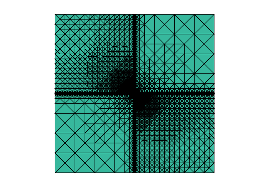
Figure 3: mesh generated by the $Z\!Z$ indicatot $\xi_{{}_{K}}^{{}_{Z\!Z}}$

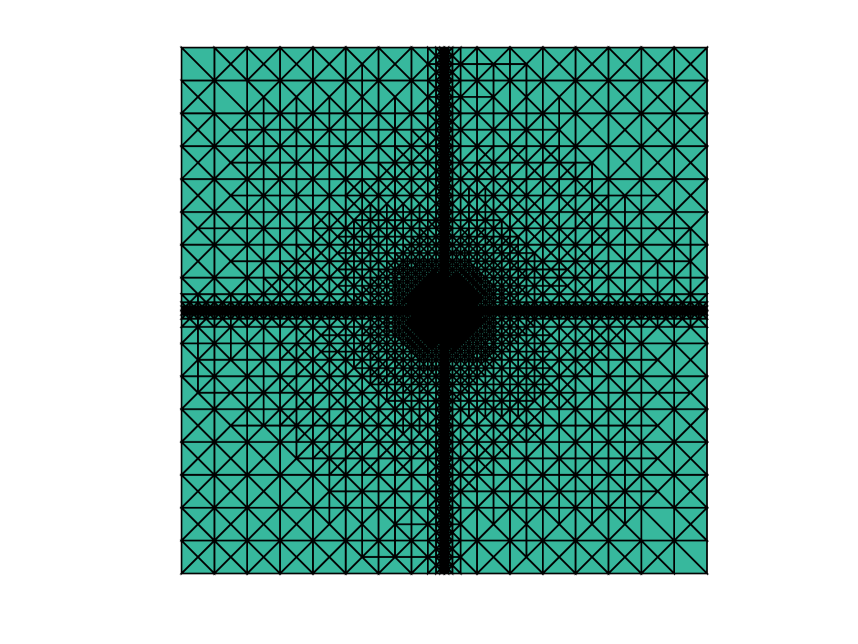
Figure 4: mesh generated by the modified $Z\!Z$ indicator $\tilde{\xi}_{{}_{K}}^{{}_{Z\!Z}}$

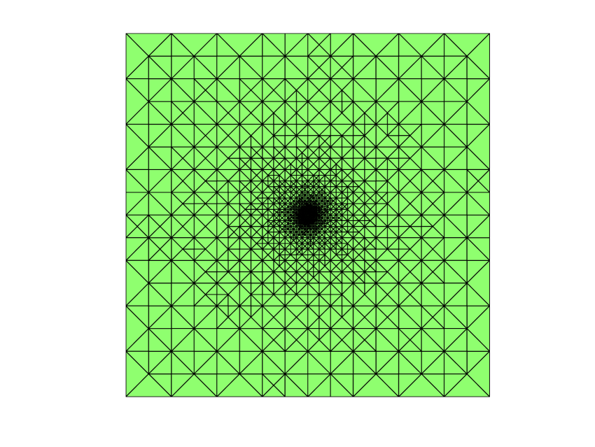
Figure 5: mesh generated by $\xi^{rt}_{{}_{K}}$

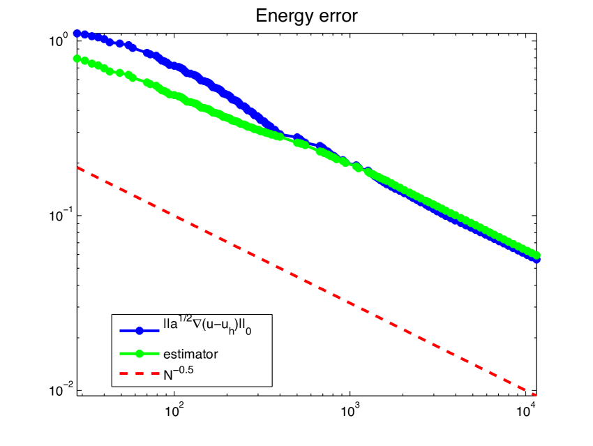
Figure 6: error and estimator $\xi^{rt}$

Figure 7: mesh generated by $\xi^{bdm}_{{}_{K}}$

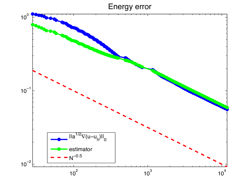
Figure 8: error and estimator $\xi^{bdm}$

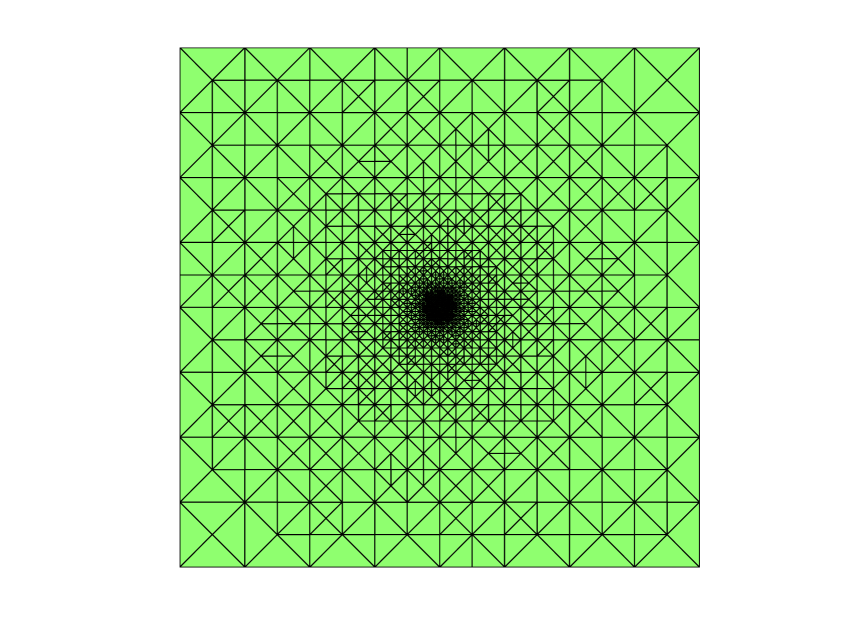
Figure 9: mesh generated by $\xi^{rt}_{{}_{F}}$

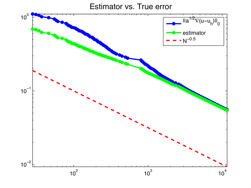
Figure 10: error and estimator $\hat{\xi}^{rt}$

Figure 11: mesh generated by $\xi^{bdm}_{{}_{F}}$

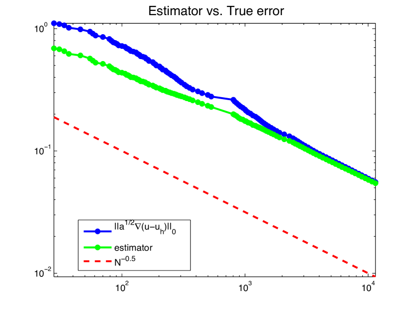
Figure 12: error and estimator $\hat{\xi}^{bdm}$

Meshes generated by $\xi_{{}_{K}}$ and $\xi_{{}_{F}}$ for both $RT$ and $B\!D\!M$ recovery are shown in Figures 6,8, 10 and 12 , respectively. The refinements are centered at the origin and there is no over-refinements along the interfaces. Similar meshes for this test problem generated by other error estimators can be found in [8, 9, 11]. The comparisons between the true error in the energy norm and the estimators, $\xi$ and $\hat{\xi}$, are shown in Figures 6, 8, 10, and 12, respectively. All the estimators have effectivity indexes very close to one. Here, the effectivity index is defined as the ratio of the estimator and the true error in the energy norm. Moreover, the slope of the log(dof)- log (the relative error) for both $\xi$ and $\hat{\xi}$ are very close to $-1/2$, which indicates the optimal decay of the error with respect to the number of unknowns.

References

[1]M. Ainsworth and J. T. Oden,
A Posteriori Error Estimation in Finite Element Analysis,
John Wiley & Sons, 2000.
[2]C. Bahriawati and C. Carstensen,Three Matlab implementations of the lowest-order Raviart-Thomas MFEM with a posteriori error control,
Comput. Methods Appl. Math., 5:4 (2005), 333-361.
[3]I. Babuška and T. Strouboulis,
The Finite Element Method and Its Reliability,
Numer. Math. Sci. Comput., Oxford Science Publication, New York, 2001.
[4]R. Bank and J. Xu,
Asymptotically exact a posteriori error estimators,
SIAM J. Numer. Anal, 41:6 (2003).
Part I: Grids with superconvergence, 2294-2312;
Part II: General unstructured grids, 2313-2332.
[5]R. Bank, J. Xu, and B. Zhang,
Superconvergent derivative recovery for Lagrange triangular elements of degree p on unstructured grids,
SIAM J. Numer. Anal., 45:5 (2007), 2032-2046.
[6]C. Bernardi and R. Verfürth,
Adaptive finite element methods for elliptic equations with non-smooth coefficients,
Numer. Math., 85:4 (2000), 579-608.
[7]D. Boffi, F. Brezzi, and M. Fortin,
Mixed Finite Element Methods and Applications,
Springer, Heidelberg, 2013.
[8]Z. Cai and S. Zhang,
Recovery-based error estimator for interface problems: conforming linear elements,
SIAM J. Numer. Anal., 47:3 (2009), 2132-2156.
[9]Z. Cai and S. Zhang,
Recovery-based error estimator for interface problems: mixed and nonconforming elements,
SIAM J. Numer. Anal., 48:1 (2010), 30-52.
[10]Z. Cai and S. Zhang,
Robust residual- and recovery a posteriori error estimators for interface problems with
flux jumps, Numer. Methods for PDEs, 28:2 (2012), 476-491.
[11]Z. Cai and S. Zhang,
Robust equilibrated residual error estimator for diffusion problems: Conforming elements,
SIAM J. Numer. Anal., 50:1 (2012), 151-170.
[12]C. Carstensen and S. Bartels,
Each averaging technique yields reliable a posteriori error control
in FEM on unstructured grids. Part I: low order conforming, nonconforming,
and mixed FEM,
Math. Comp., 71 (2002), 945-969.
[13]C. Carstensen, S. Bartels, and R. Klose,
An experimental survey of a posteriori Courant finite element error
control for the Poisson equation,
Adv. Comput. Math., 15 (2001), 79-106.
[14]C. Carstensen and R. Verfürth,
Edge residuals dominate a posteriori error estimates for low order
finite element methods,
SIAM J. Numer. Anal., 36:5 (1999), 1571-1587.
[15]P. G. Ciarlet,
The Finite Element Method for Elliptic Problems,
North-Holland, New York, 1978.
[16]W. Hoffmann, A. H. Schatz, L. B. Wahlbin, and G. Wittum,
Asymptotically exact a posteriori estimators for the pointwise gradient
error on each element in irregular meshes. Part I: a smooth problem and globally
quasi-uniform meshes,
Math. Comp., 70 (2001), 897-909.
[17]R. B. Kellogg,
On the Poisson equation with intersecting interfaces,
Appl. Anal., 4 (1975), 101-129.
[18]R. Luce and B. I. Wohlmuth,
A local a posteriori error estimator based on equilibrated fluxes,
SIAM J. Numer. Anal., 42:4 (2004), 1394-1414.
[19]A. Naga and Z. Zhang,
The polynomial-preserving recovery for higher order finite element methods
in 2D and 3D,
Discrete Contin. Dyn. Syst. Ser. B, 5:30 (2005), 769-798.
[20]J. S. Ovall,
Two Dangers to Avoid when Using Gradient Recovery Methods for Finite
Element Error Estimation and Adaptivity, Technical report 6,
Max-Planck-Institute f̈ur Mathematick in den Naturwissenschaften, Bonn, Germany, 2006.
[21]J. S. Ovall,
Fixing a “Bug” in Recovery-Type a Posteriori Error Estimators, Technical report
25, Max-Planck-Institute für Mathematick in den Naturwissenschaften, Bonn, Germany, 2006.
[22]M. Petzoldt, A posteriori error estimators for elliptic
equations with discontinuous coefficients,
Adv. Comp. Math., 16:1 (2002), 47-75.
[23]R. Rodriguez,
Some remarks on Zienkiewicz-Zhu estimator,
Int. J. Numer. Meth. PDE, 10 (1994), 625-635.
[24]A. H. Schatz and L. B. Wahlbin,
Asymptotically exact a posteriori estimators for the pointwise
gradient error on each element in irregular meshes. Part II:
the piecewise linear case,
Math. Comp., 73 (2004), 517-523.
[25]R. Verfürth,
A Posteriori Error Estimation Techniques for Finite Element Methods,
Numer. Math. Sci. Comput., Oxford University Press, Oxford, UK, 2013
[26]N. Yan and A. Zhou,
Gradient recovery type a posteriori error estimates for
finite element approximations on irregular meshes.
Part 1, Comput. Methods Appl. Mech. Engrg., 123 (1995), 173-187;
Part 2, Comput. Methods Appl. Mech. Engrg., 163 (1998), 159-170.
[27]S. Zhang,
An efficient implementation of Brezzi-Douglas-Marini (BDM) mixed finite element method in MATLAB,
arXiv:1508.06445 [math.NA], 2015.
[28]Z. Zhang,