Bosonization approach for “atomic collapse” in graphene

Abstract

We study quantum electrodynamics with 2+1 dimensional massless Dirac fermion around a Coulomb impurity. Around a large charge with atomic number Z > 137, the QED vacuum is expected to collapse due to the strong Coulombic force. While the relativistic quantum mechanics fails to make reliable predictions for the fate of the vacuum, the heavy ion collision experiment also does not give clear understanding of this system. Recently, the “atomic collapse” resonances were observed on graphene where an artificial nuclei can be made. In this paper, we present our nonperturbative study of the vacuum structure of the quasiparticles in graphene with a charge impurity which contains multi-body effect using bosonization method.

OU-HET-865

1 Introduction

The quantum electrodynamics (QED) is the most precisely experimentally tested theory in today’s fundamental theories. In usual perturbation theory of QED, the expansion parameter is the fine structure constant $\alpha\sim\frac{1}{137}$. However, in strong external field, since the interaction is correspondingly strong, the perturbation theory breaks down. From the result of relativistic quantum mechanics, the vacuum around an atom with large atomic number $Z\gtrsim 137$ is expected to collapse.

In non relativistic quantum mechanics, in the region where the potential is larger than the energy, the wave function falls off exponentially. Namely, all the incoming particles are reflected; that is, the reflection rate is $R=1$ and transmision rate is $T=0$. On the other hand, in relativistic quantum mechanics, when height of the potential $V_{0}$ is larger than twice of particle mass $2m$, the reflection rate becomes larger than unity ($R>1$), which is called the Klein tunnelingKlein:1929zz ; Bjorken:1964 . This mechanism originates from the fact that the Dirac equation has both the positive and negative energy solutions as opposed to the Schrd̈ingier equation. The same mechanism also prevents the electron to form bound states in a very strong attractive potential. In particular, an electron around a nuclei with a sufficiently large atomic number $Z$ does not form a bound state due to the strong Coulomb potential, and fall into the nuclei. This phenomenon is called the atomic collapse, and has been known theoretically for a long time. However, since the atom with $Z\gtrsim 137$ can be created for only a short time in heavy ion collision experiment, it is difficult to observe the phenomena experimentally at the quantitive level Schweppe:1983yv ; Cowan:1985cn .

The situation has changed since the discovery of the graphene in 2004Novoselov:2004 . The electric structure of the graphene at low energy is known to be the same as that of the massless Dirac fermion. In addition, the effective fine structure constant $\alpha$ is about $300$ times as large as that in the Quantum Electro Dynamics (QED). Due to this property, the essential point of the physics in the strongly coupled QED can be tested in the experiment using the graphene. Putting charged impurities on the graphene, one can realize a system similar to the large $Z$ atom system, which enable us to observe the “atomic collapse”.

The graphene is very thin, very light, very strong, and has very high electron conductivity and made from carbon atoms which is a ubiquitous element on earth. Therefore the graphene is expected to serve as ideal device in future. In this point of view, understanding the response of the electron to the charged impurity in graphene is a very important problem and is studied actively. This system is well studied in one body quantum mechanics as the system of the two dimensional massless electron in Coulomb potential Pereira:2007 ; Shytov:2007a ; Nishida:2014 . It is predicted that when the charge of the impurity exceeds a critical value $Z_{cr}$, the wave function drastically changes. The massless fermion forms infinite number of quasibound states with negative energy, and the characteristic resonances appear in the local density of states (LDOS) of the electronShytov:2007b . Inspired by these theoretical studies, the scanning tunneling microscope (STM) experiment was carried out and a characteristic peak in LDOS was measuredWang:2013 .

However, the above theoretical studies do not take into account the many body effect which involve electron-positron pair creation. In the graphene case, since the pair creation can occur with no cost of extra energy, the many body effect should not be neglected, which should be treated in the quantum field theory. Moreover, because of the large coupling perturbative approximation cannot be valid. Thus, this problem should be studied in some nonperturbative way.

We analyze the field theory of 2+1 dimensional Dirac massless fermion around an external charge using the bosonization technique. In two dimensional theory, the fermion theory is converted to the boson theoryColeman:1974bu ; Mandelstam:1975hb . It is known that a part of quantum effect of the fermion theory can be extracted from the classical boson theory. The bosonization method has been used to analyze the system with the fermion around monopole assuming that the classical boson theory captures the essential features of the quantum effect of the original fermion theoryCallan:1982au ; Harvey:1983tp . The bosonization method is applied also to the atomic collapse problem in 3+1 dimensionsHirata:1986yt . We apply this method to the atomic collapse problem in 2+1 dimensions.

Following the studies in 3+1 dimensions mentioned above, first restricting the gauge and the fermion field to s-wave field, we reduce the theory to 1+1 dimensional fermion effective theory. Next, we map the two dimensional fermion theory to the two dimensional boson theory. Then we solve the classical equation of motion for the boson field. As a result, we find the vacuum structure including the charge screening of the impurity charge.

This paper is organized as follows. In section 2, the result of foregoing analysis in one body theory for the Coulomb impurity problem on graphene is briefly reviewed. In section 3, we will explain the s-wave approximation and the bosonization formalism proposed in Ref. Hirata:1986yt . In section 4, we will show the details about our study of vacuum solution and the result of our numerical analysis. Section 5 is devoted to summary and discussion.

2 Review on Coulomb impurity on graphene

In this section, we review the Coulomb impurity problem on graphene. The electronic properties of the graphene are described by the tight-binding model where interactions between different orbits are neglected. And it is assumed that the electron can hop to only the nearest neighbor site. In momentum space, the energy of electron becomes zero at two points ($K$ and $K^{\prime}$). The low energy effective theory is obtained by expanding the equation which the electron obeys around these points. It is known that the effective Hamiltonian takes the same form as that of massless Dirac fermion. That is, the fermionic low energy excitation obeys the Dirac equation

$$-v_{F}\left(\begin{array}[]{cc}0&\hat{p_{x}}-i\hat{p_{y}}\\ \hat{p_{x}}+i\hat{p_{y}}&0\end{array}\right)\psi=\varepsilon\psi,$$ (3)

and has the linear dispersion relation

$$\varepsilon=\pm v_{F}\sqrt{p_{x}^{2}+p_{y}^{2}},$$ (4)

at low energy. The parameter $v_{F}$ in the above equation is the Fermi velocity which is roughly estimated as $v_{F}\sim\frac{c}{300}$. Since $v_{F}$ plays the similar role as the speed of light $c$ in quantum electrodynamics, the effective fine structure constant for the fermionic excitations on graphene is $\alpha_{\rm eff}\sim\frac{300}{137}$. This means that the massless Dirac fermion on graphene is strongly coupled.

The behavior of electron in a hydrogen like atom is studied in relativistic quantum mechanics. It is known that the bound state of electron and a point charge $Ze$ cannot exist when $Z\alpha\geq 1$. For such a strongly coupled system, it is expected that the strong electric field makes the vacuum unstable since the strong Coulomb potential causes particle-hole pair creations. Such a phenomenon is called the “atomic collapse” and has been discussed for a long time. In the experimental side, the atomic collapse has been tested in heavy-ion collision. However the instability of large atomic number nuclei makes it difficult to observe the phenomenon clearly.

In the graphene case, such a situation can be easily set up due to the large value of the effective coupling $\alpha\sim\frac{300}{137}$ of the Dirac fermion. Recently, Wang and his collaborators studied the graphene system with Coulomb impurities with STM and observed the resonance like the quasibound stateWang:2013 . They put Ca dimers as impurity, and measured the local density of states (LDOS) of electron around the impurity. They showed that the peak appears in energy dependence of LDOS. The peak point is below the Dirac point when 5 Ca dimers are put. According to them, this is the quasi-bound state expected in one body theory. The quasi-bound state spatially spread through about 10 nm around the center of Ca dimers in this experiment.

In view of this STM experiment, it is now very important to study the graphene system with Coulomb impurities theoretically. In one body theory, the solution of the Dirac equation with Coulomb potential by a charged impurity can be exactly obtainedPereira:2007 ; Shytov:2007a . The behavior of the solution drastically changes when $Z\alpha>1/2$. Because the electrons in graphene are massless, they do not seem to make bound state even in small $Z\alpha$. However, by introducing graphene lattice cutoff, the quasi-stable bound state is predicted to appear in strong coupling case.

In Ref. Shytov:2007b , the existence of the quasi-bound state is semiclassically discussed. Here, we briefly review their discussion. The Hamiltonian for 2 dimensional massless fermion in Coulomb potential is

$$H={\boldsymbol{\sigma}}\cdot{\bf p}-\frac{Z\alpha}{r}.$$ (5)

When we write the square of momentum in terms of the radial momentum $p_{r}$ and the angular momentum $j$

$$p^{2}=p_{r}^{2}+j^{2}/r^{2},$$ (6)

the Hamiltonian (5) leads to

$$p^{2}_{r}=\left(\varepsilon+\frac{Z\alpha+j}{r}\right)\left(\varepsilon+\frac{Z\alpha-j}{r}\right),$$ (7)

where $\varepsilon$ is energy eigenvalue. The classically forbidden region where $p_{r}^{2}<0$ corresponds to

$$r_{1}\equiv\frac{Z\alpha-j}{|\varepsilon|}<r<\frac{Z\alpha+j}{|\varepsilon|}\equiv r_{2}.$$ (8)

Notice that if $Z\alpha>j$, there exist classically allowed region inside; that is, $r<r_{1}$. Therefore in strongly coupled case, quasibound states can be found by imposing the Bohr-Sommerfeld quantization condition

$$\int_{r_{0}}^{r_{1}}p_{r}dr=n\pi,$$ (9)

where $r_{0}$ is the lattice cutoff.

In one particle theory, the interesting feature mentioned above can be found and LDOS can be calculated. However, since the atomic collapse is a phenomenon which comes from pair creation effect, it should be analyzed in a way which contain nonperturbative multi body effects. In the following section, we will show the 2+1 dimensional massless fermion version of the bosonization formulation proposed in Ref. Hirata:1986yt .

3 Approximation and Formalism

In this section, we study the vacuum structure of the massless Dirac fermion system in 2+1 dimensions around a Coulomb impurity. In order to analyze the system nonperturbatively, we employ the method proposed in Ref. Hirata:1986yt for the atomic collapse QED in 3+1 dimensions. We firs restrict the theory with s-wave electromagnetic field and the lowest partial wave electron field. Under this approximation, the theory is reduced to 1+1 dimensional effective theory with time and radial degrees of freedom. We then bosonize the effective 1+1 dimensional fermion theory. Since it is known that the bosonized theory captures important part of the nonperturbative effect of the original fermion theory even at the classical level, we study the nonperturbative vacuum structure by constructing the classical solution of the bosonized theory.

3.1 1+1D Effective Theory

Since the gauge field is in 3+1 dimensions, we start from the following gauge action

$$S_{g}=\int d^{4}x\left[-\frac{1}{4}F_{\mu\nu}F^{\mu\nu}-Ze\rho(x)A_{0}\right],$$ (10)

where the charge density of impurity is spherically symmetric $\rho(x)=\rho(r,t)$, and normalized as $\int d^{3}x\rho(x)=1$. The s-wave electromagnetic field takes following form

$$A_{0}(x)=a_{0}(r,t),\ A_{i}(x)=\hat{r}_{i}a_{1}(r,t),$$ (11)

where $\hat{r}_{i}=r_{i}/r$ is $i$th component of the unit vector in radial direction. In this approximation, the gauge action becomes

$$S_{g}=\int drdt\left[2\pi r^{2}(\partial_{0}a_{1}-\partial_{r}a_{0})^{2}-4\pi Zer^{2}\rho(r,t)a_{0}\right].$$ (12)

When the graphene is on $z=0$ surface and the electron is trapped on this surface, the action for the electron coupled with the gauge field is

$$S_{f} =\int d^{4}x\left[\overline{\psi}(i{\ooalign{\hfil/\hfil\crcr$\partial$}}+e{\ooalign{\hfil/\hfil\crcr$A$}})\psi\right]\delta(z)$$ (17)

$$=\int d^{4}x\left[\psi^{\dagger}\gamma^{0}(i\gamma^{0}\partial_{0}+i\gamma^{i}\partial_{i}+e\gamma^{0}A_{0}+e\gamma^{i}A_{i})\psi\right]\delta(z).$$

where $\psi$ is 2 component Weyl spinor. We take gamma matrices as

$$\gamma^{0}=\sigma_{3},\ \gamma^{1}=i\sigma_{2},\ \gamma^{2}=-i\sigma_{1}.$$ (18)

Because we are considering $z=0$ surface and using the s-wave approximation (11), $\gamma^{3}$ disappears from (17). From now on, $i$ runs from $1$ to $2$. The fermion action becomes

$$S_{f}=\int d^{2}xdt\psi^{\dagger}\left[(i\partial_{0}+ea_{0})+\sigma^{i}(i\partial_{i}+e\hat{r}_{i}a_{1})\right]\psi.$$ (19)

We expand the fermion field $\psi$ as

$$\psi=\frac{1}{\sqrt{r}}\sum_{m,\sigma}v_{m,\sigma}(r,t)\Psi_{m,\sigma}(\varphi),$$ (20)

where $\sigma=\pm 1$ and $m$ is half integer, and

$$\Psi_{m,\sigma}=\frac{1}{\sqrt{4\pi}}\left(\begin{array}[]{c}e^{i(m-1/2)\varphi}\\ \sigma e^{i(m+1/2)\varphi}\end{array}\right).$$ (23)

is normalized as

$$\int d\varphi\Psi_{m^{\prime}\sigma^{\prime}}^{\dagger}\Psi_{m,\sigma}=\delta_{m,m^{\prime}}\delta_{\sigma,\sigma^{\prime}}.$$ (24)

Using the relation

$$\sigma_{i}\hat{r}_{i}\Psi_{m,\sigma}=\sigma\Psi_{m,\sigma},$$ (25)

we get

$$\sigma_{i}\partial_{i}\psi=\frac{1}{\sqrt{r}}\sum_{m,\sigma}\sigma\left(\partial_{r}v_{m,\sigma}(r,t)\Psi_{m,\sigma}(\varphi)+\frac{m}{r}\Psi_{m,-\sigma}(\varphi)\right).$$ (26)

Therefore the action for fermion becomes

$$S_{f}=\int drdt\sum_{m,\sigma}\left[v_{m,\sigma}^{*}\left\{i\partial_{0}+ea_{0}+\sigma(i\partial_{r}+ea_{1})\right\}v_{m,\sigma}-i\sigma v_{m,\sigma}^{*}\frac{m}{r}v_{m,-\sigma}\right].$$ (27)

We restrict ourself to consider only the lowest ($j=1/2$) partial wave, and define 1+1 dimensional fermion

$$u_{m} :=\left(\frac{1+i}{2}+\frac{1-i}{2}\sigma_{3}\right)\left(\begin{array}[]{c}v_{m,+}\\ {\rm sign}(m)v_{m,-}\end{array}\right)$$ (30)

$$=\left(\begin{array}[]{c}v_{m,+}\\ {\rm sign}(m)iv_{m,-}\end{array}\right),$$ (33)

where $m=\pm 1/2$. From now on, we take

$$\gamma^{0}=\sigma_{2},\ \gamma^{1}=i\sigma_{1},\ \gamma_{5}=\gamma^{0}\gamma^{1}=\sigma_{3}$$ (34)

as 2 dimensional gamma matrices. Then we can rewrite 2 dimensional fermion action as

$$S_{f}=\int drdt\sum_{m=\pm 1/2}\left[\overline{u}_{m}\left\{\gamma^{0}(i\partial_{0}+ea_{0})+\gamma^{1}(i\partial_{r}+ea_{1})\right\}u_{m}+i\frac{1}{2r}\overline{u}_{m}\gamma^{5}u_{m}\right].$$ (35)

The last term represents centrifugal force. Unlike that of Ref. Hirata:1986yt ,we have a different coefficient of centrifugal force term and no mass term.

We have to set the boundary condition for fermion field $u_{m}$ at $r=0$ by requiring no singularity at $r=0$. From (23),

$$\Psi_{1/2,+}-\Psi_{1/2,-},\ \Psi_{-1/2,+}+\Psi_{-1/2,-}$$ (36)

has $\varphi$ dependence. If the coefficients of these are finite value at $r=0$, the singularity arises. So, we set the boundary condition

$$v_{m,+}(0,t)-{\rm sign}(m)v_{m,-}(0,t)=0.$$ (37)

Written in 2D fermion $u_{m}$,

$$(1-\gamma^{0})u_{m}(0,t)=0.$$ (38)

On the other hand, since

$$\Psi_{1/2,+}+\Psi_{1/2,-},\ \Psi_{-1/2,+}-\Psi_{-1/2,-}$$ (39)

don’t have $\varphi$ dependence, the coefficient of these can be finite at $r=0$. Therefore we can also use the same boundary condition as Ref. Hirata:1986yt .

By the way, in one body theory, the boundary condition is set not at $r=0$, but at $r=r_{0}$Pereira:2007 ; Shytov:2007a , which is lattice cut off size of graphene. And the cut off plays very important role to discuss the drastic change of wave function and quasi-bound state in strong coupling region. In our case, however, even if we set the boundary condition at $r=r_{0}$, we get the same result for $r=0$. Therefore, here we set the boundary condition at $r=0$.

3.2 Bosonization

We apply bosonization to this theory. Regarding interaction term as perturbation, we bosonize free fermion field to free boson field,

$$u_{m}(r,t)=\left(\frac{\mu}{2\pi}\right)^{1/2}\left(\begin{array}[]{c}-iN_{\mu}\exp[i\sqrt{\pi}(\phi_{m}(r,t)+\tilde{\phi}_{m}(r,t))]\\ N_{\mu}\exp[i\sqrt{\pi}(-\phi_{m}(r,t)+\tilde{\phi}_{m}(r,t))]\end{array}\right),$$ (42)

where

$$\tilde{\phi}(x)=\lim_{\epsilon\to 0}\int_{r}^{\infty}dse^{-\epsilon s}\dot{\phi}(s,t),$$ (43)

and $N_{\mu}$ represents normal ordering at IR mass scale $\mu$. From now on, we use the overdot and prime for time and spatial derivative, respectively. Because the action and the boundary condition are almost the same as Ref. Hirata:1986yt , we can bosonize this theory following the same calculation.

In this case, we should impose the boundary condition on the boson field. The boundary condition (38) is rewritten in boson field as

$$\phi_{m}(0,t)=0.$$ (44)

Free boson field can be expanded in plane wave as

$$\phi(x,t)=\int_{k>0}\frac{dk}{2\pi}\left[\bar{a}^{\dagger}(k)e^{ik(x+t)}+a(k)e^{ik(x-t)}+\bar{a}(k)e^{-ik(x+t)}+a^{\dagger}(k)e^{-ik(x-t)}\right],$$ (45)

where $a,\ \bar{a},\ a^{\dagger},\ \bar{a}^{\dagger}$ are creation-annihilation operators satisfying appropriate commutation relations. While $a(k),\bar{a}(k)$ are independent operators without the boundary condition, with the boundary condition (44)

$$0 =\phi(0,t)$$

$$=\int_{k>0}\frac{dk}{2\pi}\left[(\bar{a}^{\dagger}(k)+a^{\dagger}(k))e^{ikt}+(a(k)+\bar{a}(k))e^{-ikt}\right],$$ (46)

these are dependent on each other

$$\bar{a}(k)=-a(k).$$ (47)

Then the boson field $\phi$ and $\tilde{\phi}$ can be written as

$$\phi(r,t)=\int_{k>0}\frac{dk}{2\pi}\left[a(k)(e^{ikr}-e^{-ikr})e^{-ikt}+a^{\dagger}(k)(e^{-ikr}-e^{ikr})e^{ikt}\right],$$ (48)

and

$$\tilde{\phi}(r,t)=\int_{k>0}\frac{dk}{2\pi}\left[\left(e^{ikr}+e^{-ikr}\right)a(k)e^{-ikt}+\left(e^{ikr}+e^{-ikr}\right)a^{\dagger}(k)e^{ikt}\right].$$ (49)

We split these into

$$\phi^{(+)}(r,t)=\int_{k>0}\frac{dk}{2\pi}a(k)\left(e^{ikr}-e^{-ikr}\right)e^{-ikt},$$ (50)

$$\phi^{(-)}(r,t)=\int_{k>0}\frac{dk}{2\pi}a^{\dagger}(k)\left(e^{-ikr}-e^{ikr}\right)e^{ikt},$$ (51)

$$\tilde{\phi}^{(+)}(r,t)=\int_{k>0}\frac{dk}{2\pi}a(k)\left(e^{ikr}+e^{-ikr}\right)e^{-ikt},$$ (52)

$$\tilde{\phi}^{(-)}(r,t)=\int_{k>0}\frac{dk}{2\pi}a^{\dagger}(k)\left(e^{ikr}+e^{-ikr}\right)e^{ikt}.$$ (53)

From the commutation relation $[a(k),a^{\dagger}(k)]=2\pi\frac{1}{2k}\delta(k-k^{\prime})$, we get the relation

$$[\tilde{\phi}^{(+)}(r,t)+\eta\phi^{(+)}(r,t),\tilde{\phi}^{(-)}(r^{\prime},t^{\prime})+\eta^{\prime}\phi^{(-)}(r^{\prime},t^{\prime})]$$

$$\qquad=-\frac{1}{4\pi}[(1-\eta)(1-\eta^{\prime})A_{+}+(1+\eta)(1+\eta^{\prime})A_{-}+(1-\eta)(1+\eta^{\prime})B_{+}+(1+\eta)(1-\eta^{\prime})B_{-}],$$ (54)

where

$$A_{\pm}(r,t;r^{\prime},t^{\prime}) \equiv-\int_{k>0}dk\frac{1}{k}e^{ik(\mp(r-r^{\prime})-(t-t^{\prime}))}$$

$$=\lim_{\epsilon\to 0}\ln\left(i\mu[t-t^{\prime}\pm(r-r^{\prime})-i\epsilon\right]),$$ (55)

$$B_{\pm}(r,t;r^{\prime},t^{\prime}) \equiv-\int_{k>0}dk\frac{1}{k}e^{ik(\mp(r+r^{\prime})-(t-t^{\prime}))}$$

$$=\lim_{\epsilon\to 0}\ln\left(i\mu[t-t^{\prime}\pm(r+r^{\prime})-i\epsilon\right]),$$ (56)

are renormalized at IR mass scale $\mu$. $B_{+,-}$ arise from the boundary condition.

Using the commutation relation (54), we rewrite the interaction terms in fermion theory in terms of boson field. After some point splitting procedure, we get

$$\overline{u}\gamma^{\mu}u=-\frac{1}{\sqrt{\pi}}\epsilon^{\mu\nu}\partial_{\nu}\phi,$$ (57)

$$\overline{u}\gamma_{5}u=-\frac{i}{2\pi r}N_{\mu}\cos(2\sqrt{\pi}\phi),$$ (58)

where $\epsilon$ is anti-symmetric symbol with $\epsilon^{10}=1$.

We rewrite the fermion action (35) in terms of the above boson operators. In $a_{1}=0$ gauge,

$$S_{f}=\int drdt\sum_{m=\pm 1/2}\left[\frac{1}{2}\partial^{\mu}\phi_{m}\partial_{\mu}\phi_{m}-\frac{e}{\sqrt{\pi}}a_{0}^{\prime}\phi_{m}+\frac{1}{4\pi r^{2}}\cos(2\sqrt{\pi}\phi_{m})\right],$$ (59)

where the second term is integrated by parts. Therefore we get the total action

$$S=\int drdt\left[2\pi r^{2}a_{0}^{\prime 2}+e\Phi(r,t)a_{0}^{\prime}+\sum_{m=\pm 1/2}\left(\frac{1}{2}\partial^{\mu}\phi_{m}\partial_{\mu}\phi_{m}-\frac{e}{\sqrt{\pi}}a_{0}^{\prime}\phi_{m}+\frac{1}{4\pi r^{2}}\cos(2\sqrt{\pi}\phi_{m})\right)\right],$$ (60)

where the $\Phi(r,t)$ is defined by

$$\Phi^{\prime}(r,t)=4\pi Zr^{2}\rho(r,t).$$ (61)

From the action (60), we notice that $a_{0}$ has no dynamical degrees of freedom. Using the equation of motion for $a^{\prime}_{0}$

$$4\pi r^{2}a_{0}^{\prime}+e\Phi(r,t)-\sum_{m=\pm 1/2}\frac{e}{\sqrt{\pi}}\phi_{m}=0,$$

we can eliminate $a_{0}$. Therefore the Hamiltonian becomes

$$H=\int dr\left[\sum_{m=\pm 1/2}\left\{\frac{1}{2}\left(\pi_{m}^{2}+\phi_{m}^{\prime 2}\right)-\frac{1}{4\pi r^{2}}\cos(2\sqrt{\pi}\phi_{m})\right\}+\frac{e^{2}}{8\pi r^{2}}\left(\Phi(r,t)-\frac{1}{\sqrt{\pi}}\sum_{m}\phi_{m}\right)^{2}\right].$$ (62)

Adding the c-number to the Hamiltonian,

$$H =\int dr\left[\sum_{m=\pm 1/2}\left\{\frac{1}{2}\left(\pi_{m}^{2}+\phi_{m}^{\prime 2}\right)+\frac{1}{4\pi r^{2}}\left(1-\cos(2\sqrt{\pi}\phi_{m})\right)\right\}\right.$$

$$\qquad\left.+\frac{e^{2}}{8\pi r^{2}}\left\{\left(\Phi(r,t)-\frac{1}{\sqrt{\pi}}\sum_{m}\phi_{m}\right)^{2}-\Phi(r,t)^{2}\right\}\right],$$ (63)

we shift the energy so that the energy becomes zero when $\phi_{m}=0$ which is vacuum configuration with $Z=0$. In the next section, we numerically calculate the solution which minimize this Hamiltonian.

4 Study of Vacuum Solution

In this section we find the classical solution which minimizes the bosonized Hamiltonian in the previous section. For this purpose, we have to solve the Euler-Lagrange equations for boson fields under the appropriate boundary conditions. The boundary condition at $r=0$ is determined by eq.(44). The solution is characterized by the boundary condition at $r=\infty$.

Eq.(57) indicates that the density of electron $\rho_{e}(r)$ can be written in terms of the boson field as

$$\rho_{e}(r) \equiv\psi^{\dagger}\psi=\sum_{m}\frac{1}{\sqrt{\pi}}\partial_{r}\phi_{m}(r).$$ (64)

Therefore, we get the spatial distribution of induced electron density corresponding to the solution. Total induced charge which screens the impurity charge is given by

$$Q_{\mathrm{EM}} \equiv-e\int dr\rho_{e}(r)=-\frac{e}{\sqrt{\pi}}\sum_{m}\phi_{m}(\infty).$$ (65)

In order to study the vacuum structure, we consider only static solution $\pi_{m}=0$. We rewrite the Hamiltonian in terms of the new variable

$$\phi_{\pm}=\frac{1}{\sqrt{2}}(\phi_{+1/2}\pm\phi_{-1/2}).$$ (66)

Using the formula

$$\cos[\sqrt{2\pi}(\phi_{+}+\phi_{-})]+\cos[\sqrt{2\pi}(\phi_{+}-\phi_{-})]=2\cos(\sqrt{2\pi}\phi_{+})\cos(\sqrt{2\pi}\phi_{-}),$$ (67)

the Hamiltonian becomes

$$H =\int_{0}^{\infty}dr\left[\frac{1}{2}(\phi^{\prime 2}_{+}+\phi_{-}^{\prime 2})+\frac{1}{2\pi r^{2}}\{1-\cos(\sqrt{2\pi}\phi_{+})\cos(\sqrt{2\pi}\phi_{-})\}\right.$$

$$\qquad\left.+\frac{\alpha}{\pi r^{2}}\left\{\left(\phi_{+}-\sqrt{\frac{\pi}{2}}\Phi(r,t)\right)^{2}-\frac{\pi}{2}\Phi(r,t)^{2}\right\}\right],$$ (68)

where $\alpha=\frac{e^{2}}{4\pi}$. The Euler-Lagrange equations for $\phi_{+},\phi_{-}$ are given by

$$\phi_{+}^{\prime\prime}-\frac{1}{\sqrt{2\pi}r^{2}}\sin(\sqrt{2\pi}\phi_{+})\cos(\sqrt{2\pi}\phi_{-})-\frac{2\alpha}{\pi r^{2}}\left(\phi_{+}-\sqrt{\frac{\pi}{2}}\Phi(r)\right)=0,$$ (69)

$$\phi_{-}^{\prime\prime}-\frac{1}{\sqrt{2\pi}r^{2}}\cos(\sqrt{2\pi}\phi_{+})\sin(\sqrt{2\pi}\phi_{-})=0,$$ (70)

respectively. Since it satisfies Eq.(70) we can take the symmetric ansatz $\phi_{-}=0$. Then Eq.(69) reduces to

$$\phi_{+}^{\prime\prime}-\frac{1}{\sqrt{2\pi}r^{2}}\sin(\sqrt{2\pi}\phi_{+})-\frac{2\alpha}{\pi r^{2}}\left(\phi_{+}-\sqrt{\frac{\pi}{2}}\Phi(r)\right)=0.$$ (71)

We assume that the impurity charge is spherically spread over radius $R$:

$$\rho(r)=\frac{3}{4\pi R^{3}}\theta(R-r).$$ (72)

The corresponding $\Phi(r)$ is

$$\Phi(r)=\left\{\begin{array}[]{cc}Z\left(\frac{r}{R}\right)^{3}&\quad(r<R)\\ Z&\quad(r>R).\end{array}\right.$$ (75)

Since Eq.(71) is a second order differential equation, in addition to the boundary condition at the origin we need to impose another boundary condition at $r=\infty$. For finiteness of total energy, the boson field should asymptotically be constant ($\phi_{+}\rightarrow\phi_{*}$) at large $r$. Substituting $\phi_{+}=\phi_{*}$ into the Euler-Lagrange equation at large $r$, we find that $\phi_{*}$ should be the solution of the following equation:

$$\sin(\sqrt{2\pi}\phi_{*})=-2\alpha\left(\sqrt{\frac{2}{\pi}}\phi_{*}-Z\right).$$ (76)

Notice that the asymptotic value $\sqrt{\frac{2}{\pi}}\phi_{*}$ can take non-integer value. Charge screening with non-integer charge may seem counter intuitive if one tries to interpret the phenomena as particle hole pair creation. One should interpret such screening as the polarization effect.

In fact, it is known that the screening of non-integer charge actually occurs in massless Schwinger model Callan:1982au ; Rubakov:1983vn ; Iso:1988zi . In the following subsections, we show the detailed numerical analysis and its results.

4.1 Numerical Analysis

4.1.1 Strategy

Our numerical analysis is done in various parameters $\alpha,Z$, according to the following steps:

(i)

Find the solution of Eq.(76) and obtain the asymptotic form at large $r$.

(ii)

Solve the Euler-Lagrange equation (71) with the boundary condition at large $r$ (82) with various $A$.

(iii)

Find $A$ with which the solution satisfies the boundary condition at $r=0$ (44).

4.1.2 Asymptotic form

In order to numerically solve the Euler-Lagrange equation (71), we should find the asymptotic form at large $r$. To do so, we parameterize $\phi_{+}(r)$ by introducing a function $f$ which describes the deviation of $\phi_{+}(r)$ and $\phi_{*}$ at large $r$ as

$$\phi_{+}(r)=\phi_{*}-f(r).$$ (77)

where $\phi_{*}$ is the solution of Eq.(76). Substituting Eq.(77) into Eq.(71), and expanding it up to linear order in $f$, we obtain

$$f^{\prime\prime}-\frac{1}{r^{2}}\left(\cos(\sqrt{2\pi}\phi_{*})+\frac{2\alpha}{\pi}\right)f+O(f^{2})=0$$ (78)

Assuming that the solution for $f$ can take the form

$$f(r)\approx\frac{A}{r^{\lambda}},$$ (79)

at large $r$ with $A$ being a constant and substituting it into Eq.(78), we find that the power $\lambda$ satisfies the following equation:

$$\lambda^{2}+\lambda-\left(\cos(\sqrt{2\pi}\phi_{*})+\frac{2\alpha}{\pi}\right)=0.$$ (80)

From Eq.(80), $\lambda$ should be

$$\lambda=\frac{1}{2}\left[-1+\sqrt{1+4\cos(\sqrt{2\pi}\phi_{*})+\frac{8\alpha}{\pi}}\right].$$ (81)

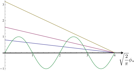
Figure 1: The green line is l.h.s. of eq.(76), and blue, red, yellow lines are r.h.s. of eq.(76) with $\alpha=0.1$, $\alpha=0.2$, $\alpha=0.4$, respectively.

We show some examples of $Z=4$ case. In this case, there are three screening patterns depending on the value of $\alpha$ as shown in Fig. 1. In $\alpha\lesssim 0.14$ case, there are five values of $\phi_{*}$. However, when $\phi_{*}$ is equal to the second or fourth smallest value, based on Eq.(81), $\lambda$ becomes imaginary. Only the solutions with the real positive values of $\lambda$ make sense. So, there are three possibilities. For $0.14\lesssim\alpha\lesssim 0.34$ case, there are three values of $\phi_{*}$. Similarly the second smallest value of $\phi_{*}$ is not a physical solution. So, there are two possibilities. And in $0.34\lesssim\alpha$ case, there is only value for $\phi_{*}$ which corresponds to the full screening solution.

In Fig. 2, we show the number of possible asymptotic solutions at large $r$ for each set of values of ($\alpha$, $Z$).

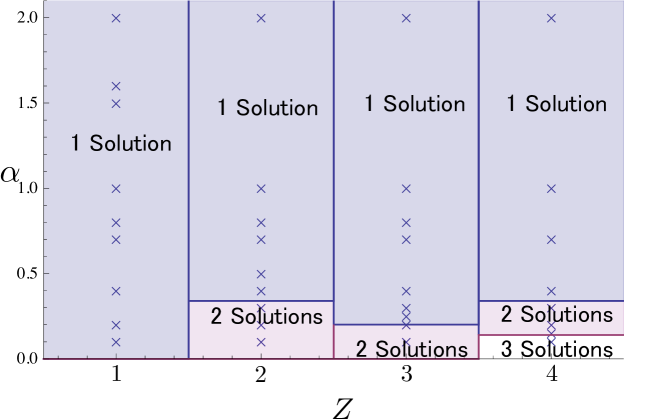
Figure 2: Number of possible asymptotic solutions at large $r$ for each set of values of ($\alpha$, $Z$). Crosses are the parameter points where we solved Eq. (71)

4.1.3 Example of the solution

Starting from the asymptotic solutions and solving the differential equation numerically, we can obtain the full solution. Taking the following asymptotic from

$$\phi_{+}(r)\approx\phi_{*}-\frac{A}{r^{\lambda}},$$ (82)

at large $r$ and varying $A$, we can search for the physical solution which satisfies the boundary condition at $r=0$. Practically, we solve Eq. (71) from $r=0.001R$ to $r=100000R$, setting the boundary condition at large $r=100000R$ with various values of $\alpha,Z$. For illustration, we show the example for $Z=4$ and $\alpha=0.2$. In this case, there are two asymptotic solutions, but only the solution which realizes the smallest value of $\phi_{*}$ can satisfy appropriate boundary condition. The full solutions from the other asymptotic forms do not satisfy the boundary condition at $r=0$ but end up have positive values no matter how we choose the value of $A$. We show the solution of $\phi_{+}(r)$ in Fig. 4. In the other case, the shapes of solutions are qualitatively similar to the solution in this case. The induced electron density is depicted in Fig. 4. We notice that most of the induced electrons fall into the impurity.

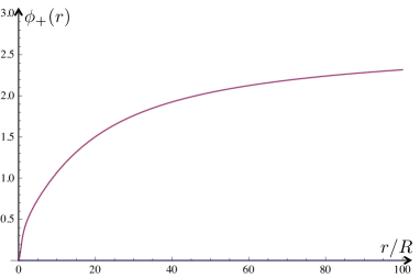
Figure 3: The solution for $\alpha=0.2,Z=4$.

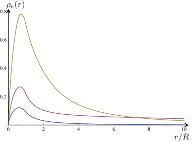
Figure 4: Induced electron density with $\alpha=0.1$ (blue line), $\alpha=0.2$ (red line), $\alpha=0.4$ (yellow line).

4.2 Result

4.2.1 Phase structure

We looked for the solution for various set of parameters of ($\alpha,Z$), where the parameter set is given in Fig. 2 . We found that only the solution with the smallest value of $\phi_{*}$ can satisfy correct boundary condition at $r=0$ in all cases. From this fact, we reach the conjecture that the magnitude of screening can be determined by the smallest intersection of $\sin(\sqrt{2\pi}\phi_{*})$ and $-2\alpha(\sqrt{2/\pi}\phi_{*}-Z)$. According to this conjecture, we get effective impurity charge seen from infinitely separated point,

$$Z_{\rm eff}=Z-\sqrt{\frac{2}{\pi}}\phi_{*},$$ (83)

which is screened by induced charge Fig. 5. Notice that when $\alpha\gtrsim 0.2$, the effective impurity charge $Z_{\rm eff}$ in any odd $Z$ case is the same one as in $Z=1$ case. Also when $\alpha\gtrsim 0.14$, $Z_{\rm eff}$ in any even $Z$ case is the same one as in $Z=2$ case. From this result, a phase diagram of screening is described as in Fig. 6. In larger $Z$ case, more branches appear in small $\alpha$ regime.

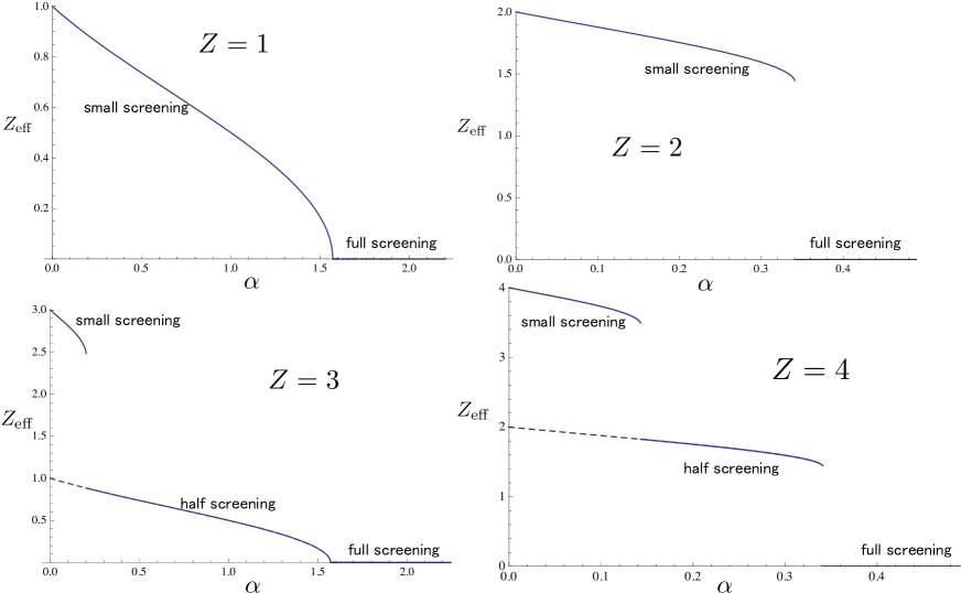
Figure 5: $Z_{\rm eff}$ for each $Z$. Dashed lines in $Z=3,4$ cases describe $Z_{\rm eff}$ in $Z=1,2$ cases, respectively.

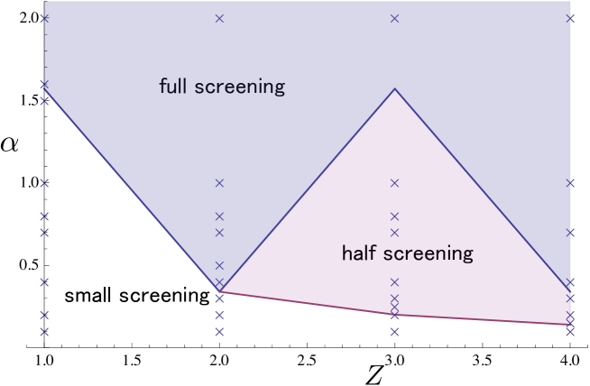
Figure 6: Phase diagram of screening. Crosses are the parameter points where we solved Eq. (71)

4.2.2 Scaling law

The induced 2D electron density can be obtained as

$$n(r)=\frac{\rho_{e}(r)}{2\pi r}.$$ (84)

If graphene sheet can be treated as perfect metal, the scaling law is calculated as in Ref. Fogler:2007 :

$$n(r)\propto r^{-3},$$ (85)

in the range of distances $1\ll r/R\ll 2\alpha^{2}Z$. In our calculation, we fit the scaling law

$$n(r)\propto r^{-\gamma}$$ (86)

in the range of distances $1\ll r/R\ll 10$. The scaling exponent $\gamma$ depends on parameters $\alpha,Z$ as shown in Fig.7. In small screening regime, we get $\gamma\sim 2.7$, independently of $\alpha$. Near the value of $\alpha$ where magnitude of screening jumps, $\gamma$ drastically decreases. In larger $\alpha$ regime, $\gamma$ increases and becomes close to the value calculated in perfect metal approximation.

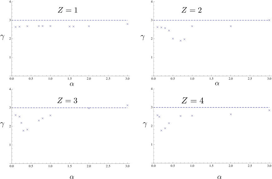
Figure 7: Crosses describe the scaling exponent in each $Z$ case. Dashed line describes one in perfect metal approximation.

5 Summary and Discussion

In this paper, we studied quantum field theory with the 2+1 dimensional massless fermion around an external Coulomb field. We reduced the theory to a two dimensional fermion theory, where the higher partial waves are neglected. Bosonizing the theory, we have found the static solution of classical equation of motion for the boson field. The magnitude of screening is determined only by the asymptotic equation of motion. Which of these asymptotic solutions satisfies the boundary condition at $r=0$ is determined by dynamics.

Through the study of several examples, we have concluded that the realized solution is always the smallest screening one. As a result, we have found patterns of screening depending on the coupling $\alpha$ and the impurity charge $Z$. The screening charge undergoes a drastic change as we change the value of $\alpha$ at some critical values. We also obtained the phase diagram characterized by the patterns of screening.

By solving the equation of motion in full spatial regime, we have obtained the spatial distribution of density of the induced electron. The radial profile of the two dimensional induced charge density can be fitted by negative power in $r$ which is the distance from the impurity. In weak coupling regime, scaling exponent $\gamma$ is independent of $\alpha$ and $Z$; $\gamma\approx 2.7$. Near the screening jumping point, $\gamma$ decreases. This means that the induced fermion is widely spread near the screening jumping point. And in larger $\alpha$ regime, $\gamma$ become close to the value of the perfect metal approximation; $\gamma\approx 3$.

The validity of the approximation to neglect higher partial wave can be discussed somewhat in semi classical theory mentioned in section 2. According to the semi classical theory, only $Z\alpha>j$ wave can form quasi-bound states. So, the fermion mode whose angular momentum $j$ is higher than $Z\alpha$ is irrelevant to anomalous behavior of the electron in strong Coulomb potential. When $Z\alpha>3/2$, the next to lowest partial wave $j=3/2$ should be relevant to this problem. Therefore our approximation should be valid only when $Z\alpha<3/2$.

To compare our analysis with the result of one particle theory or the experiment, many things remain to be done. Validity of classical treatment for boson theory should be confirmed quantitatively. In Ref. Hirata:1989px , the bosonized atomic collapse problem in 3+1 dimensions is treated within small fluctuation approximation. They show the existence of meta stable states in supercritical phase. In the same way it may be possible to show the existence of the meta stable states in our 2+1 dimensional massless fermion case.

The contribution of higher momentum partial wave should be evaluated for understanding larger $\alpha,Z$ case. Furthermore to understand the behavior in the regime closer to the impurity, the effect of graphene lattice should be considered. For that purpose, the simulation by lattice gauge theory is important.

- (1) O. Klein, Die Reflexion von Elektronen an einem Potentialsprung nach der relativistischen Dynamik von Dirac, Z. Phys. 53 (1929) 157.
- (2) J. D. Bjorken and S. D. Drell, Relativistic Quantum Mechanics(McGrawHill, New York, 1964).
- (3) J. Schweppe, A. Gruppe, K. Bethge, H. Bokemeyer, T. Cowan, H. Folger, J. S. Greenberg and H. Grein et al., Observation of a peak structure in positron spectra from U + Cm collisions, Phys. Rev. Lett. 51 (1983) 2261.
- (4) T. Cowan, H. Backe, M. Begemann, K. Bethge, H. Bokemeyer, H. Folger, J. S. Greenberg and H. Grin et al., Anomalous positron peaks from supercritical collisions systems, Phys. Rev. Lett. 54 (1985) 1761.
- (5) K.S. Novoselov, A.K. Geim, S.V. Morozov, D. Jiang, Y. Zhang, S.V. Dubonos, I.V.Grigorieva, A.A. Firsov, Electric Field Effect in Atomically Thin Carbon Films, Science 306(2004) 666.
- (6) Vitor M. Pereira, Johan Nilsson, and A. H. Castro Neto, Coulomb Impurity Problem in Graphene, Phys. Rev. Lett. 99 (2007) 166802.
- (7) A. V. Shytov, M. I.Katsnelson, L. S. Levitov, Vacuum Polarization and Screening of Supercritical Impurities in Graphene, Phys. Rev. Lett. 99 (2007) 236801.
- (8) Y. Nishida, Vacuum polarization of graphene with a supercritical Coulomb impurity: Low-energy universality and discrete scale invariance, Phys. Rev. B 90 (2014) 165414.
- (9) A. V. Shytov, M. I.Katsnelson, L. S. Levitov, Atomic Collapse and Quasi-Rydberg States in Graphene, Phys. Rev. Lett. 99 (2007) 246802.
- (10) Wang, Yang, et al. Observing Atomic Collapse Resonances in Artificial Nuclei on Graphene,Science 340 (2013) 734.
- (11) S. R. Coleman, The Quantum Sine-Gordon Equation as the Massive Thirring Model, Phys. Rev. D 11 (1975) 2088.
- (12) S. Mandelstam, Soliton Operators for the Quantized Sine-Gordon Equation, Phys. Rev. D 11 (1975) 3026.
- (13) C. G. Callan, Jr., Dyon-Fermion Dynamics, Phys. Rev. D 26 (1982) 2058.
- (14) J. A. Harvey, Magnetic Monopoles With Fractional Charges, Phys. Lett. B 131 (1983) 104.
- (15) Y. Hirata and H. Minakata, Quantum Field Theories Around a Large Nucleus, Phys. Rev. D 34 (1986) 2493.
- (16) V. A. Rubakov, On the Vacuum Structure in Quantum Electrodynamics With Massless Fermions, Nucl. Phys. B 236 (1984) 109.
- (17) S. Iso and H. Murayama, Hamiltonian Formulation of the Schwinger Model: Nonconfinement and Screening of the Charge, Prog. Theor. Phys. 84 (1990) 142.
- (18) M. M. Fogler, D. S. Novikov and B. I. Shklovskii Screening of a hypercritical charge in graphene, Phys. Rev. B 76 (2007) 233402.
- (19) Y. S. Hirata and H. Minakata, Quantum Field Theories Around a Large Nucleus. 2. Metastable States in Supercritical Phase, Z. Phys. C 46 (1990) 45.