CP Violation in $\mathbf{D^{0}\rightarrow K_{S}K_{S}}$

Abstract

The direct CP asymmetry $a_{CP}^{\mathrm{dir}}(D^{0}\rightarrow K_{S}K_{S})$ involves exchange diagrams which are induced at tree level in the Standard Model. Since the corresponding topological amplitude $E_{KK}$ can be large, $D^{0}\rightarrow K_{S}K_{S}$ is a promising discovery channel for charm CP violation. We estimate the penguin annihilation amplitude with a perturbative calculation and extract the exchange amplitude $E_{KK}$ from a global fit to $D$ branching ratios. Our results are further used to predict the size of mixing-induced CP violation. We obtain $|a_{CP}^{\mathrm{dir}}(D^{0}\rightarrow K_{S}K_{S})|\leq 1.1\%$ (95% C.L.). The same bound applies to the nonuniversal part of the phase between the $D\!-\!\,\overline{\!D}{}\,$ mixing and decay amplitudes. If future data exceed our predictions, this will point to new physics or an enhancement of the penguin annihilation amplitude by QCD dynamics. We briefly discuss the implications of these possibilities for other CP asymmetries.

I Introduction

While direct CP violation (CPV) is well established in the down-quark sector Fanti et al. (1999); Lai et al. (2001); Batley et al. (2002); Alavi-Harati et al. (1999, 2003); Lin et al. (2008); Duh et al. (2013); Aubert et al. (2007); Lees et al. (2013); Abulencia et al. (2006); Aaltonen et al. (2011), CPV has not yet been observed in the decays of up-type quarks. For the discussion of CPV in some singly Cabibbo-suppressed $D$ decay it is convenient to decompose the decay amplitude $\mathcal{A}$ as

$$\mathcal{A} =\lambda_{sd}\mathcal{A}_{sd}-\frac{\lambda_{b}}{2}\mathcal{A}_{b}.$$ (1)

Here $\lambda_{q}\equiv V_{cq}^{*}V_{uq}$ and $\lambda_{sd}=(\lambda_{s}-\lambda_{d})/2$ comprise the elements $V_{ij}$ of the Cabibbo-Kobayashi-Maskawa (CKM) matrix. In the limit $\lambda_{b}=0$ all direct and mixing-induced CP asymmetries vanish in the Standard Model (SM). The suppression factor $\mbox{Im}\,\frac{\lambda_{b}}{\lambda_{sd}}\sim-6\cdot 10^{-4}$ makes the discovery of CKM-induced CPV challenging. At the same time this parametric suppression renders CP asymmetries in charm decays highly sensitive to physics beyond the SM.

In this paper we study the decay $D^{0}\to K_{S}K_{S}$. For this decay mode $\mathcal{A}_{sd}$ vanishes in the limit of exact SU(3)_F symmetry Buccella et al. (1995); Bhattacharya and Rosner (2010); Brod et al. (2012); Hiller et al. (2013), so that the branching ratio is suppressed. However, $\mathcal{A}_{b}$ does not vanish in this limit and we expect $|\mathcal{A}_{b}/\mathcal{A}_{sd}|$ to be large. Therefore CP asymmetries in $D^{0}\to K_{S}K_{S}$ may be enhanced to an observable level, even if the Kobayashi-Maskawa phase is the only source of CPV in charm decays Brod et al. (2012); Hiller et al. (2013). Moreover, a special feature of $D^{0}\to K_{S}K_{S}$ is the interference of the decays $c\overline{u}\to\overline{s}s$ and $c\overline{u}\to\overline{d}d$, both of which involve the tree-level exchange of a $W$ boson (exchange topology $E$, see Fig. 1). This interference term gives a contribution to $\mathcal{A}_{b}$ owing to $\lambda_{d}+\lambda_{s}=-\lambda_{b}$. That is, contrary to the widely studied decays $D\to\pi^{+}\pi^{-},\pi^{0}\pi^{0},K^{+}K^{-}$, no penguin diagrams are needed for nonzero direct or mixing-induced CP asymmetries. Moreover, the exchange diagram $E$ is enhanced by a large Wilson coefficient. These properties make $D^{0}\to K_{S}K_{S}$ an interesting discovery channel for CPV in the charm system.

In this paper we calculate the allowed ranges for the direct and mixing-induced CP asymmetries in $D^{0}\to K_{S}K_{S}$, using the results of our global analysis in Ref. Müller et al. (2015a). There are two ingredients which we cannot extract from this analysis: the first one is the penguin-annihilation amplitude $PA$ (see Fig. 1), which we estimate with the help of a perturbative calculation. The other undetermined quantity is a strong phase $\delta$, whose value, however, can be determined from the data once both the direct and mixing-induced CP asymmetries are measured. The actual size of $\delta$ is not crucial for the potential to discover charm CPV in $D^{0}\to K_{S}K_{S}$: depending on whether $|\sin\delta|$ is large or small either the direct or mixing-induced CP asymmetry will be large.

Our paper is organized as follows: in Section II we derive handy formulae for direct and mixing-induced CP asymmetries in terms of $\mathcal{A}_{sd}$ and $\mathcal{A}_{b}$. In Section III we relate the CPV observables to topological amplitudes. Subsequently we estimate the penguin annihilation contribution, which cannot be extracted from a global fit to current data, with perturbative methods in Section IV. In Section V we present our phenomenological analysis. Finally, we conclude.

II Preliminaries

In this section we collect the formulae for the CP asymmetries. We write

$$\mathcal{A}(D^{0}\rightarrow K_{S}K_{S})=-\frac{1}{\sqrt{2}}\,\mathcal{A}(D^{0}\rightarrow\bar{K}^{0}K^{0})\,,$$ (2)

accommodating the Bose symmetrization of the two $K_{S}$’s with the factor of $1/\sqrt{2}$. Here we identify $K_{S}=(K^{0}-\overline{K}{}^{0})/\sqrt{2}$ and assume that the effects of kaon CPV are properly subtracted from CP asymmetries measured in $D^{0}\to K_{S}K_{S}$, as described in Ref. Grossman and Nir (2012). Adopting the convention $CP\left|{D^{0}}\right\rangle=-\left|{\overline{D}{}^{0}}\right\rangle$ Gersabeck et al. (2012) the amplitude of $\overline{D}{}^{0}\to K_{S}K_{S}$ is

$$\overline{\mathcal{A}} =-\lambda_{sd}^{*}\mathcal{A}_{sd}+\frac{\lambda_{b}^{*}}{2}\mathcal{A}_{b}.$$ (3)

The direct CP asymmetry reads

$$a_{CP}^{\mathrm{dir}} \equiv\frac{|\mathcal{A}|^{2}-|\overline{\mathcal{A}}|^{2}}{|\mathcal{A}|^{2}+|\overline{\mathcal{A}}|^{2}}$$ (4)

$$=\frac{\mathrm{Im}\,\lambda_{b}}{|\mathcal{A}|}\;\mathrm{Im}\frac{\mathcal{A}_{b}}{\mathcal{A}_{sd}}|\mathcal{A}_{sd}|\,.$$ (5)

Here and in the following we neglect terms of order $\lambda_{b}^{2}$ and higher. Furthermore we use the PDG convention for the CKM elements, so that $\lambda_{sd}$ is real and positive up to corrections of order $\lambda_{b}$.

For the discussion of mixing-induced CPV we also follow the conventions of Ref. Gersabeck et al. (2012): with the mass eigenstates $\left|{D_{1,2}}\right\rangle=p\left|{D^{0}}\right\rangle\pm q\left|{\overline{D}^{0}}\right\rangle$ we define the weak phase $\phi$ governing CPV in the interference between the $D\!-\!\,\overline{\!D}{}\,$ mixing and the $D^{0}\to K_{S}K_{S}$ decay through

$$\frac{q}{p}\frac{\overline{\mathcal{A}}}{\mathcal{A}} =-\frac{q}{p}\,\frac{\lambda_{sd}^{*}}{\lambda_{sd}}\,\frac{\displaystyle 1-\frac{\lambda_{b}^{*}}{2\lambda_{sd}^{*}}\frac{\mathcal{A}_{b}}{\mathcal{A}_{sd}}}{\displaystyle 1-\frac{\lambda_{b}}{2\lambda_{sd}}\frac{\mathcal{A}_{b}}{\mathcal{A}_{sd}}}$$

$$\equiv\left|\frac{q}{p}\right|\,\left|\frac{\overline{\mathcal{A}}}{\mathcal{A}}\right|\,e^{i\phi}\,.$$ (6)

In this paper we focus on CPV effects which are specific to the decay $D^{0}\to K_{S}K_{S}$. It is therefore useful to define a CP phase $\phi_{\mathrm{mix}}$ which enters all mixing-induced CP asymmetries in a universal way:

$$-\frac{q}{p}\,\frac{\lambda_{sd}^{*}}{\lambda_{sd}} \equiv\left|\frac{q}{p}\right|e^{i\phi_{\mathrm{mix}}}\,.$$ (7)

Comparing Eqs. (6) and (7) one verifies that $\phi_{\mathrm{mix}}$ coincides with $\phi$ if one sets $\lambda_{b}$ to zero in $\overline{\mathcal{A}}/\mathcal{A}$. In the hunt for new physics (NP) in $D\!-\!\,\overline{\!D}{}\,$ mixing, which may well enhance $\phi_{\mathrm{mix}}$ over the SM expectation $\phi_{\mathrm{mix}}={\cal O}({\mbox{Im}\,}\lambda_{b}/\lambda_{sd})$, one fits the CPV data of all available $D^{0}$ decays to a common phase $\phi_{\mathrm{mix}}$ Grossman et al. (2007); Amhis et al. (2012). In the case of $D^{0}\to K_{S}K_{S}$, however, we face the possibility that already the SM contributions lead to the situation $|\phi|\gg|\phi_{\mathrm{mix}}|$. Comparing Eq. (6) with Eq. (7) one finds

$$\frac{\displaystyle 1-\frac{\lambda_{b}^{*}}{2\lambda_{sd}^{*}}\frac{\mathcal{A}_{b}}{\mathcal{A}_{sd}}}{\displaystyle 1-\frac{\lambda_{b}}{2\lambda_{sd}}\frac{\mathcal{A}_{b}}{\mathcal{A}_{sd}}} =\left|\frac{\overline{\mathcal{A}}}{\mathcal{A}}\right|\,e^{i(\phi-\phi_{\mathrm{mix}})}$$

$$=\left(1-a_{CP}^{\mathrm{dir}}\right)\,e^{i(\phi-\phi_{\mathrm{mix}})}\,,$$ (8)

where we have used Eq. (4), discarding higher-order terms $\sim(a_{CP}^{\mathrm{dir}})^{2}$ as usual. By expanding Eq. (8) to first order in $\lambda_{b}$ and $\phi-\phi_{\mathrm{mix}}$ we arrive at

$$\phi-\phi_{\mathrm{mix}} =\mbox{Im}\,\frac{\lambda_{b}}{\lambda_{sd}}\mbox{Re}\,\frac{\mathcal{A}_{b}}{\mathcal{A}_{sd}}=\frac{\mathrm{Im}\,\lambda_{b}}{|\mathcal{A}|}\;\mathrm{Re}\frac{\mathcal{A}_{b}}{\mathcal{A}_{sd}}|\mathcal{A}_{sd}|\,.$$ (9)

Eqs. (5) and (9) form the basis of the analysis presented in the following sections. In Eqs. (5) and (9) $|\mathcal{A}|$ is trivially related to the well-measured branching ratio:

$$|\mathcal{A}| =\sqrt{\frac{\mathcal{B}(D\rightarrow K_{S}K_{S})}{\mathcal{P}(D,K,K)}}\,,$$

$$\mathcal{P}(D,K,K) \equiv\tau\,\frac{1}{16\pi m_{D}^{2}}\sqrt{m_{D}^{2}-4m_{K^{0}}^{2}}\,,$$ (10)

The experimental value is $\mathcal{B}(D^{0}\rightarrow K_{S}K_{S})=(0.17\pm 0.04)\cdot 10^{-3}$ Beringer et al. (2012). The nontrivial quantities entering the predictions of $a_{CP}^{\mathrm{dir}}$ and $\phi-\phi_{\mathrm{mix}}$ are $\mathcal{A}_{b}$ and the phase of $\mathcal{A}_{sd}$.

The time-dependent CP asymmetry reads

$$A_{CP}(t) =\frac{\Gamma(D^{0}(t)\to K_{S}K_{S})-\Gamma(\overline{D}{}^{0}(t)\to K_{{S}}K_{S})}{\Gamma(D^{0}(t)\to K_{{S}}K_{S})+\Gamma(\overline{D}{}^{0}(t)\to K_{{S}}K_{S})}$$

$$=a_{CP}^{\mathrm{dir}}-A_{\Gamma}\frac{t}{\tau}\,.$$ (11)

Here $\tau$ is the $D^{0}$ lifetime and

$$A_{\Gamma}{=}\left[\frac{1}{2}\left(\left|\frac{q}{p}\right|^{2}-1\right)-a_{CP}^{\mathrm{dir}}\right]y\cos\phi-x\sin\phi\,.$$ (12)

Eq. (12) contains the mass difference $\Delta M$ and the width difference $\Delta\Gamma$ between the mass eigenstates $D_{1}$ and $D_{2}$ through $x=\tau\Delta M$ and $y=\tau\Delta\Gamma/2$. In Eqs. (11) and (12) all quadratic (and higher) terms in tiny quantities are neglected. In time-integrated measurements, LHCb measures the quantity Gersabeck et al. (2012); Aaij et al. (2014, 2015)

$$A_{CP} =a_{CP}^{\mathrm{dir}}-A_{\Gamma}\frac{\langle t\rangle}{\tau},$$ (13)

where $\langle t\rangle$ is the average decay time. CLEO has measured Bonvicini et al. (2001)

$$A_{CP}^{\mathrm{CLEO}} =-0.23\pm 0.19.$$ (14)

Recently LHCb has reported the preliminary result M. Alexander for the LHCb collaboration

$$A_{CP}^{\mathrm{LHCb}} =-0.029\pm 0.052\pm 0.022\,.$$ (15)

III Topological amplitudes

The decomposition of $\mathcal{A}_{sd}$ and $\mathcal{A}_{b}$ in terms of topological amplitudes reads Müller et al. (2015a)

$$\mathcal{A}_{sd} =\frac{E_{1}+E_{2}-E_{3}}{\sqrt{2}}\,,$$ (16)

$$\mathcal{A}_{b} =\frac{2E+E_{1}+E_{2}+E_{3}+PA}{\sqrt{2}}$$ (17)

$$=-\mathcal{A}_{sd}+\frac{2E_{KK}+PA}{\sqrt{2}}\,.$$ (18)

Here $E_{KK}\equiv E+E_{1}+E_{2}$ is the combination of exchange diagrams appearing in $D^{0}\rightarrow K^{+}K^{-}$. The exchange ($E$) and penguin annihilation ($PA$) diagrams are shown in Fig. 1. $E_{1,2,3}$ account for first-order SU(3)_F breaking in diagrams containing $s$-quark lines (for their precise definition see Table II of Ref. Müller et al. (2015a)). As in Ref. Müller et al. (2015b) $PA_{q}$ denotes the penguin annihilation diagram with quark $q$ running in the loop. We use the combinations Golden and Grinstein (1989); Pirtskhalava and Uttayarat (2012); Hiller et al. (2013)

$$\lambda_{s} PA_{s}+\lambda_{d}PA_{d}+\lambda_{b}PA_{b}=$$

$$\;\lambda_{sd}(PA_{s}-PA_{d})+\frac{\lambda_{s}+\lambda_{d}}{2}\,\,(PA_{s}+PA_{d}-2PA_{b})$$ (19)

$$\equiv\lambda_{sd}PA_{\mathrm{break}}-\frac{\lambda_{b}}{2}PA\,.$$ (20)

We recall that $E$, $E_{1,2,3}$, $PA$,…are defined for $D^{0}\to K^{0}\overline{K}{}^{0}$ or $D^{0}\to K^{+}K^{-}$. Since $\mathcal{A}_{sd}$ and $\mathcal{A}_{b}$ instead involve $K_{S}K_{S}$, the factor of $-1/\sqrt{2}$ of Eq. (2) appears in Eqs. (16) to (18).

Next we define the strong phase

$$\delta\equiv\mathrm{arg}\left(\frac{2E_{KK}+PA}{A_{sd}}\right)\,,$$ (21)

and the positive quantity

$$R ={-\frac{\mathrm{Im}\lambda_{b}}{|\mathcal{A}|}}\frac{|2E_{KK}+PA|}{\sqrt{2}}.$$ (22)

With Eq. (18) we can write Eq. (9) as

$$\phi-\phi_{\mathrm{mix}} =\mbox{Im}\,\frac{\lambda_{b}}{\lambda_{sd}}\,\mbox{Re}\,\frac{-\mathcal{A}_{sd}+(2E_{KK}+PA)/\sqrt{2}}{\mathcal{A}_{sd}}$$

$$=-\mathrm{Im}\frac{\lambda_{b}}{\lambda_{sd}}-R\cos\delta\,.$$ (23)

In the same way one finds

$$a_{CP}^{\mathrm{dir}} ={-}R\sin\delta\,.$$ (24)

Eqs. (23) and (24) mean that $a_{CP}^{\mathrm{dir}}$ and $\phi-\phi_{\mathrm{mix}}$ lie on a circle with radius $R$ centered at $(-\mathrm{Im}\frac{\lambda_{b}}{\lambda_{sd}},0)$. The allowed points are parametrized by the phase $\delta$, which we cannot predict. The actual value of $\delta$, however, is of minor importance for the discovery potential of CPV, because $\delta$ only controls how the amount of CPV is shared between $a_{CP}^{\mathrm{dir}}$ and $\phi-\phi_{\mathrm{mix}}$. The crucial parameter is $R$, which determines the maximal values of $|a_{CP}^{\mathrm{dir}}|$ and $|\phi-\phi_{\mathrm{mix}}|$. Once $a_{CP}^{\mathrm{dir}}$ and $\phi-\phi_{\mathrm{mix}}$ are precisely measured one can determine $R$ through

$$R =\sqrt{a_{CP}^{\mathrm{dir}}{}^{2}+\left(\phi-\phi_{\mathrm{mix}}+\mathrm{Im}{\frac{\lambda_{b}}{\lambda_{sd}}}\right)^{2}}\,.$$ (25)

The experimental value can then be confronted with the theoretical estimate presented in the next section. The impact of our estimate on $a_{CP}^{\mathrm{dir}}$ and $\phi-\phi_{\mathrm{mix}}$ will be presented below in Fig. 4.

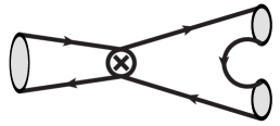
(a)

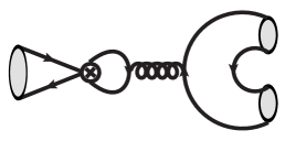
(b)

Figure 1: Topological amplitudes: (a) exchange ($E$) and (b) penguin annihilation ($PA$). Ref. Atwood and Soni (2013) claims that $D^{0}\rightarrow K_{S}K_{S}$ is Zweig suppressed, but this statement is only true for the PA diagram.

IV Estimate of $\mathbf{|PA|}$ and $\mathbf{R}$

The quantity $|E_{KK}|$ can be determined from our global fit to branching ratios Müller et al. (2015a). For the calculation of $PA$ we exploit the large momentum $\sqrt{q^{2}}\sim 1.5\,\mbox{GeV}$ flowing through the penguin loop in Fig. 1(b) and calculate this loop perturbatively as in Ref. Brod et al. (2012). Such methods are routinely used in $B$ physics Bander et al. (1979); Beneke et al. (1999, 2001); Beneke and Neubert (2003); Beneke et al. (2005); Frings et al. (2015), but their applicability to charm physics is not clear.

We work in a five-flavor theory, so that only current-current operators appear in the effective Hamiltonian. With $Q_{2}\equiv({\overline{u}s})_{V-A}(\overline{{s}}c)_{V-A}+({\overline{u}d})_{V-A}(\overline{d}c)_{V-A}-2({\overline{u}b})_{V-A}(\overline{b}c)_{V-A}$ and the Wilson coefficient $C_{2}\sim 1.2$ we may write

$$\mathcal{A}_{b} =\frac{G_{F}}{\sqrt{2}}{C_{2}}\left\langle{K_{S}K_{S}}\right|Q_{2}\left|{D^{0}}\right\rangle,$$ (26)

because the contribution of the color-flipped operator $Q_{1}$ is highly suppressed. For our estimate of the ratio $PA/E_{KK}$ in this section we adopt the SU(3)_F limit and identify $E_{KK}$ with $E$. In this limit we can combine Eqs. (26) and (17) into

$$\frac{G_{F}}{\sqrt{2}}{C_{2}}\left\langle{K_{S}K_{S}}\right|Q_{2}\left|{D^{0}}\right\rangle =\frac{2E+PA}{\sqrt{2}}\,.$$ (27)

The penguin diagram can be written as Lenz et al. (1997)

$$PA={G_{F}}\frac{\alpha_{s}}{4\pi}C_{2}\times$$

$$\quad\times\sum_{i=3}^{6}\left(r_{2i}^{d}+r_{2i}^{s}-2r_{2i}^{b}\right)\left\langle{K_{S}K_{S}}\right|Q_{i}\left|{D^{0}}\right\rangle\,,$$ (28)

with the loop function $r_{24}^{q}\equiv r_{24}^{q}(q^{2},m_{q}^{2},\mu^{2})=r_{26}^{q}$ defined in Ref. Lenz et al. (1997). $\mu\sim\sqrt{q^{2}}$ is the renormalization scale which also enters $\alpha_{s}$ and $C_{2}$ in Eq. (28). $Q_{3-6}$ are the usual four-quark penguin operators, we will need

$$Q_{4,6} =(\overline{u}{}^{\alpha}c^{\beta})_{V-A}\!\!\!\sum_{q=u,d,s,c{,b}}(\overline{q}{}^{\beta}q^{\alpha})_{V\mp A}.$$ (29)

$PA$ is color-suppressed w.r.t. $E$ and this suppression is encoded in Eq. (28) through $\alpha_{s}\sim 1/N_{c}$. The contributions from the matrix elements $\langle Q_{3,5}\rangle$ are further suppressed and are neglected in the following. We write $\langle Q_{4}\rangle+\langle Q_{6}\rangle=-2\left(M_{VA}^{{d}}+M_{VA}^{{s}}\right)$ with

$$M_{VA}^{{q}} \equiv\left\langle{K_{{S}}K_{{S}}}\right|(\bar{q}_{\alpha}q_{\beta})_{V}(\bar{u}_{\beta}c_{\alpha})_{A}\left|{D^{0}}\right\rangle\,.$$ (30)

The other quark flavors in the sum in Eq. (29) contribute to $D^{0}\to K_{{S}}K_{{S}}$ only through another loop diagram, yielding a contribution of higher order in $\alpha_{s}$. With

$$p \equiv r_{24}^{d}+r_{24}^{s}-2r_{24}^{b}\,,$$ (31)

we can write $PA$ in a compact form:

$$PA=-{G_{F}}\frac{\alpha_{s}}{\pi}C_{2}\,p\,M_{VA}^{d}\,,$$ (32)

where we have invoked the SU(3)_F limit to set $M_{VA}^{d}=M_{VA}^{s}$. The $\mu$-dependence cancels in $p$, which furthermore does not depend on $m_{c}$ in the considered leading order. It is an excellent numerical approximation to expand $p$ to first order in $m_{s}^{2}/q^{2}$ and $q^{2}/m_{b}^{2}$ (while setting $m_{d}=0$). The expanded expression reads

$$p =-\frac{10}{9}-\frac{2}{3}i\pi-\frac{2m_{s}^{2}}{q^{2}}+\frac{2q^{2}}{15m_{b}^{2}}+\frac{2}{3}\ln\frac{q^{2}}{m_{b}^{2}}{\,.}$$ (33)

It is worthwhile to discuss how this result translates into an expression in a four-flavor theory, in which the $b$ quark is integrated out at the scale $\mu_{b}={\cal O}(m_{b})$: in this alternative approach the piece $-2r_{2i}^{b}$ of Eq. (28) resides in the initial conditions of the penguin coefficients $C_{3-6}$ generated at $\mu_{b}$. The four-flavor theory permits the use of the renormalization group (RG) to resum the log $\ln(\mu_{b}/\sqrt{q^{2}})$ to all orders in perturbation theory, but this resummation is inconsistent since $\ln(\mu_{b}/\sqrt{q^{2}})$ is smaller than the nonlogarithmic terms in $-2r_{2i}^{b}$. Without RG summation the four-flavor theory reproduces exactly the analytic result in Eq. (33), which is independent of renormalization scale and scheme.

To estimate $M_{{VA}}^{{d}}$ we want to relate it to $E$ using Eq. (27). After Fierz-rearranging $Q_{2}$ we can express the LHS of Eq. (27) in terms of $M_{VA}^{q}$ and

$$M_{AV}^{{q}} \equiv\left\langle{K_{S}K_{S}}\right|(\bar{q}_{\alpha}q_{\beta})_{A}(\bar{u}_{\beta}c_{\alpha})_{V}\left|{D^{0}}\right\rangle\,.$$ (34)

The exchange topology reads (cf. Eq. (27))

$$E ={G_{F}C_{2}}\left\langle{K_{S}K_{S}}\right|({\overline{u}d})_{V-A}(\overline{d}c)_{V-A}\left|{D^{0}}\right\rangle-PA_{d}$$

$$={-G_{F}C_{2}}\left(M_{AV}^{d}+M_{VA}^{d}\right)-{G_{F}\frac{\alpha_{s}}{\pi}}C_{2}r_{24}^{d}M^{d}_{VA}\,.$$ (35)

To leading order in $\alpha_{s}$ we have therefore $E={-G_{F}C_{2}}\left(M_{AV}^{d}+M_{VA}^{d}\right)$. For the desired estimate of $PA/E$ we need $M_{VA}^{d}/E$. We can place a bound on this quantity with Eq. (35), if we assume that $|M^{d}_{VA}|$ is not much larger than $|M_{AV}^{d}+M_{VA}^{d}|$; i.e. we do not consider the case of large cancellations between $M_{AV}^{d}$ and $M_{VA}^{d}$ in $E$. In view of the fact that $E$ is numerically large Müller et al. (2015a) this assumption seems justified. Writing

$$M^{d}_{VA} =\kappa(M_{AV}^{d}+M_{VA}^{d}){\,,}$$ (36)

we vary $|\kappa|$ between 0 and 2. Now Eq. (35) entails

$$\frac{M^{d}_{VA}}{E} ={\frac{\kappa}{-G_{F}C_{2}(1+\kappa\frac{\alpha_{s}}{\pi}r_{24}^{d})}}{\,,}$$ (37)

and thus

$$\left|2E_{KK}+PA\right| =\left|2E_{KK}\right|\left|1+\frac{\alpha_{s}}{2\pi}p\frac{\kappa}{1+\kappa\frac{\alpha_{s}}{\pi}r_{24}^{d}}\right|$$ (38)

$$\leq\left|2E_{KK}\right|\times 1.3\,,$$ (39)

Here we have used $\mu=\sqrt{q^{2}}=1.5$ GeV, $m_{s}{(\mu)}=0.104$ GeV, $m_{b}{(\mu)}=4.18$ GeV, and $\alpha_{s}{(\mu)}=0.328$. ($r_{24}^{d}$ is evaluated in the NDR scheme.) Inserting finally Eq. (39) into Eq. (22) gives the upper limit

$$R\, {\leq}-{1.3}\frac{\mathrm{Im}\lambda_{b}}{|\mathcal{A}|}\frac{|2E_{KK}|}{\sqrt{2}}\,.$$ (40)

This bound determines the radius of the circle which defines the allowed area for $(\phi-\phi_{\mathrm{mix}},a_{CP}^{\mathrm{dir}})$ via Eq. (25). I.e. Eq. (40) determines the maximal size of both $|a_{CP}^{\mathrm{dir}}|$ and $|\phi-\phi_{\mathrm{mix}}|$ (neglecting the small $\mbox{Im}\,\lambda_{b}/\lambda_{sd}$ in Eq. (23)). If future data violate Eq. (40), this will signal new physics or a dynamical enhancement of $PA$ over the perturbative result in Eq. (32). Sec. V discusses how these two scenarios can be distinguished with the help of other measurements.

The relation of $r_{24}^{q}(q^{2},m_{q}^{2},\mu^{2})$ to $G(s,x)$ in Ref. Beneke et al. (2001) is given as

$$r_{24}^{q}(q^{2},m_{q}^{2},\mu^{2}) =\frac{1}{3}-\frac{1}{3}\log\left(\frac{\mu^{2}}{m^{2}}\right)$$

$$\quad{-}\frac{1}{2}G\left(\frac{m_{q}^{2}-i\varepsilon}{m^{2}},\frac{q^{2}}{m^{2}}\right)\,,$$ (41)

with an arbitrary mass $m^{2}$. Note that the $-i\varepsilon$ prescription is essential here; an erroneous omission of this small imaginary part results in a numerically large mistake. The prefactor of $G(x,y)$ in Eq. (41) disagrees with Ref. Brod et al. (2012). We further find that the $b$-quark contribution $-2r_{24}^{b}$ is numerically as important as $r_{24}^{d}+r_{24}^{s}$:

$$r_{24}^{d}(q^{2},0,\mu^{2}) =-0.22-i\,1.05\,,$$ (42)

$$r_{24}^{s}(q^{2},m_{s}^{2},\mu^{2}) =-0.23-i\,1.05\,,$$ (43)

$$-2r_{24}^{b}(q^{2},m_{b}^{2},\mu^{2}) =-2.02\,.$$ (44)

V Phenomenology

The last element needed for the calculation of our bound in Eq. (40) is $|E_{KK}|$. To find $|E_{KK}|$ we employ our global fit to all available branching ratios of $D$ decays to two pseudoscalar mesons Müller et al. (2015a). Note that the main constraint on this quantity stems from $\mathcal{B}(D^{0}\rightarrow K^{+}K^{-})$ (see Table III of Ref. Müller et al. (2015a)). The $D$ decays entering our fit involve other topological amplitudes in addition to $E$ and $PA$; in the following we refer to the color-favored tree (T), color-suppressed tree (C), annihilation (A) and penguin (P) amplitudes.

We consider two scenarios: in the first scenario the SU(3)_F-limit amplitudes $C$ and $E$ are varied completely freely. In the second scenario we apply $1/N_{c}$ counting ’t Hooft (1974); Buras et al. (1986); Buras and Silvestrini (2000) to the amplitudes, where $N_{c}=3$ is the number of colors. To leading order in $1/N_{c}$ one can factorize $T$ which results in

$$T^{\mathrm{fac}} \equiv\frac{G_{F}}{\sqrt{2}}a_{1}f_{\pi}\left(m_{D}^{2}-m^{2}_{\pi}\right)F_{0}^{D\pi}(m_{\pi}^{2})\,.$$ (45)

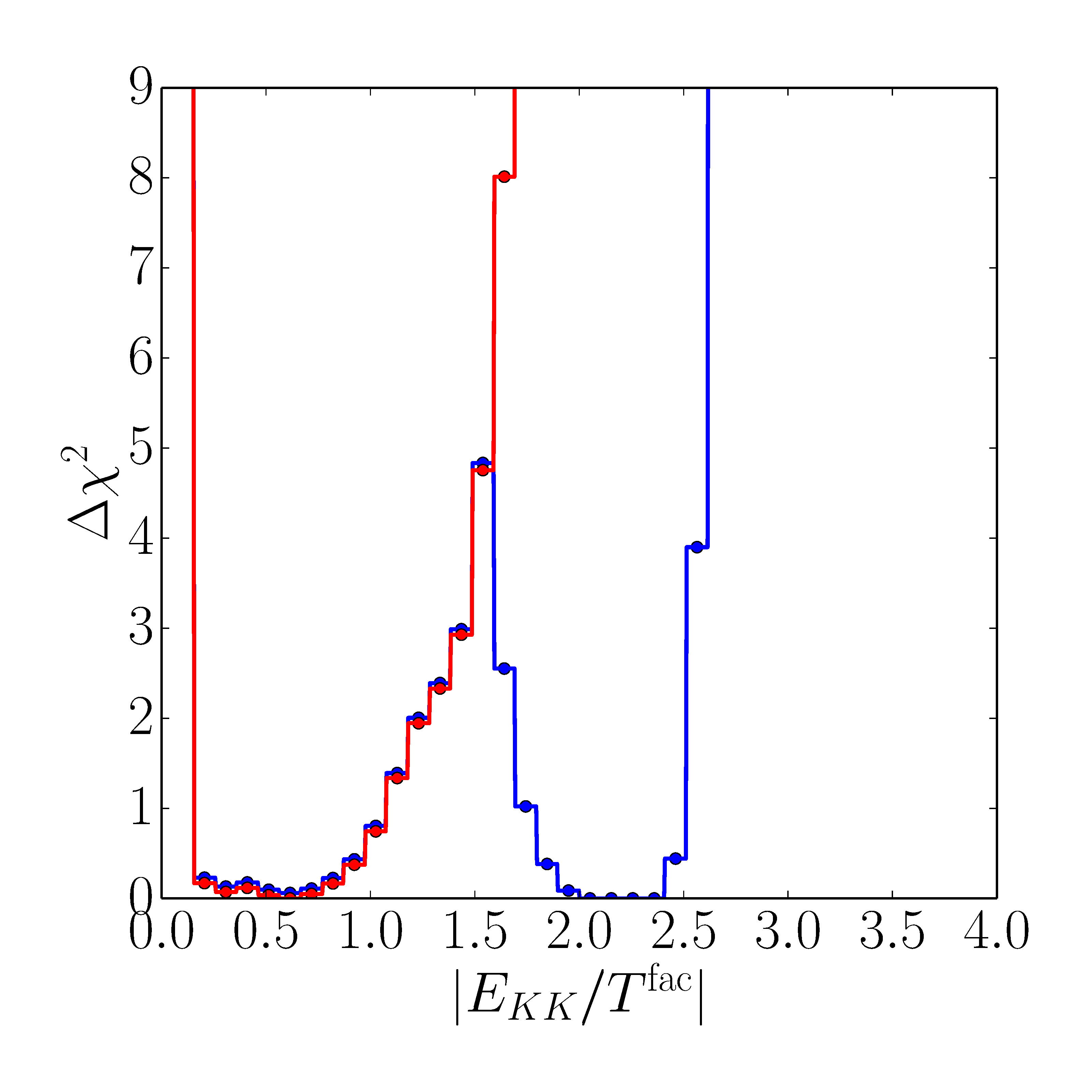
(a)

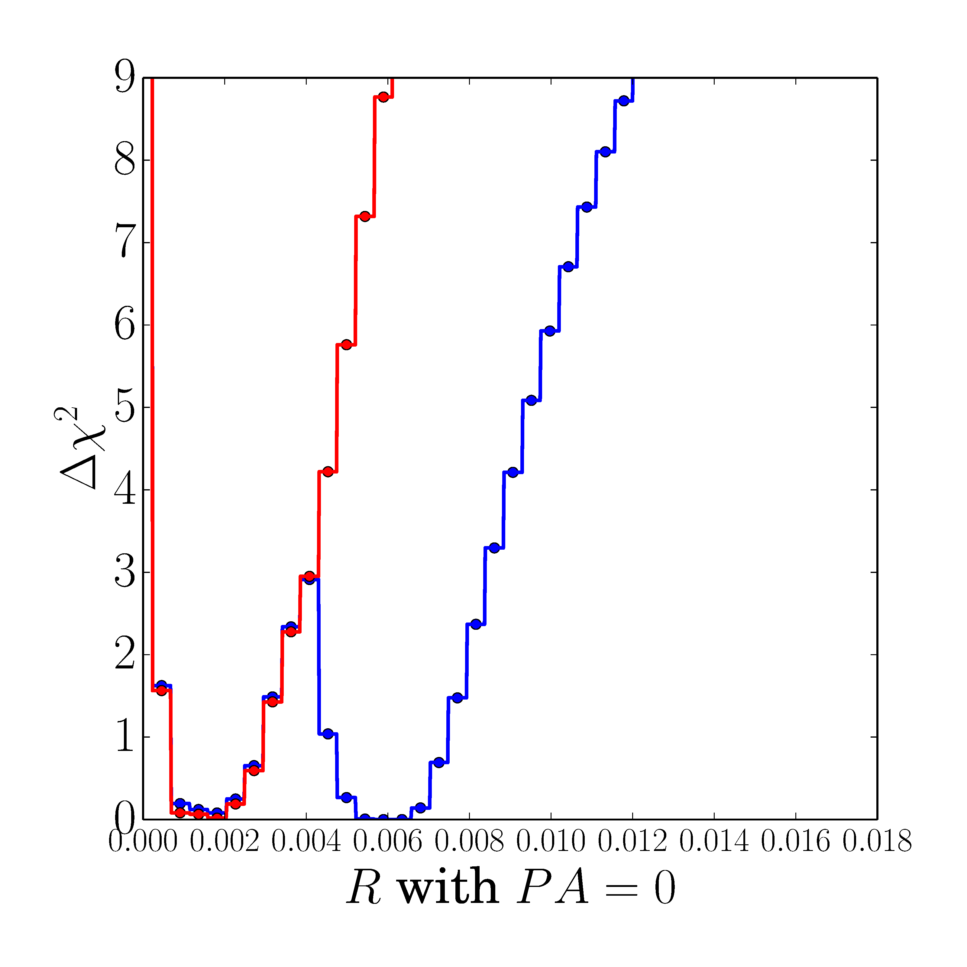
(b)

Figure 2: (a) $\Delta\chi^{2}$ profile of $|E_{KK}|$. (b) $\Delta\chi^{2}$ profile of $R$ (defined in Eq. (22)) for $PA=0$. The blue and red curves correspond to the scenarios without and with $1/N_{c}$ counting applied to $C$ and $E$. Note that the red line lies partially on top of the blue line.

Here $a_{1}=1.06$ is the appropriate combination of Wilson coefficients, $m_{\pi}$ and $f_{\pi}$ are the mass and the decay constant of the pion, respectively, and $F_{0}^{D\pi}$ is the appropriate $D\to\pi$ form factor. (Recall that the SU(3)_F-limit amplitudes are defined for decays into pions.) In our second scenario we assume that $|(C+\delta_{A})/T^{\mathrm{fac}}|,\,|(E+\delta_{A})/T^{\mathrm{fac}}|\leq 1.3$ Müller et al. (2015b), where $\delta_{A}$ parametrizes $1/N_{c}^{2}$ corrections to the factorized annihilation (A) topology Müller et al. (2015a).

The $\Delta\chi^{2}$-profile of $|E_{KK}/T^{\mathrm{fac}}|$ returned by our global fit is shown in Fig. 2(a). Fig. 2(b) shows the $\Delta\chi^{2}$-profile of $R$ for the special case $PA=0$, in which the whole effect comes from the exchange diagram $E_{KK}$. The corresponding 95% C.L. bounds on $|E_{KK}/T^{\mathrm{fac}}|$ and $R$ inferred from Fig. 2 and Eq. (40) are given in Table 1 and illustrated in Fig. 3. Note that we do not treat $T^{\mathrm{fac}}$ as constant, but also fit the form factor $F_{0}^{D\pi}$. Likewise our fit permits $\mathcal{B}(D^{0}\rightarrow K_{S}K_{S})$ to float within the experimental errors.

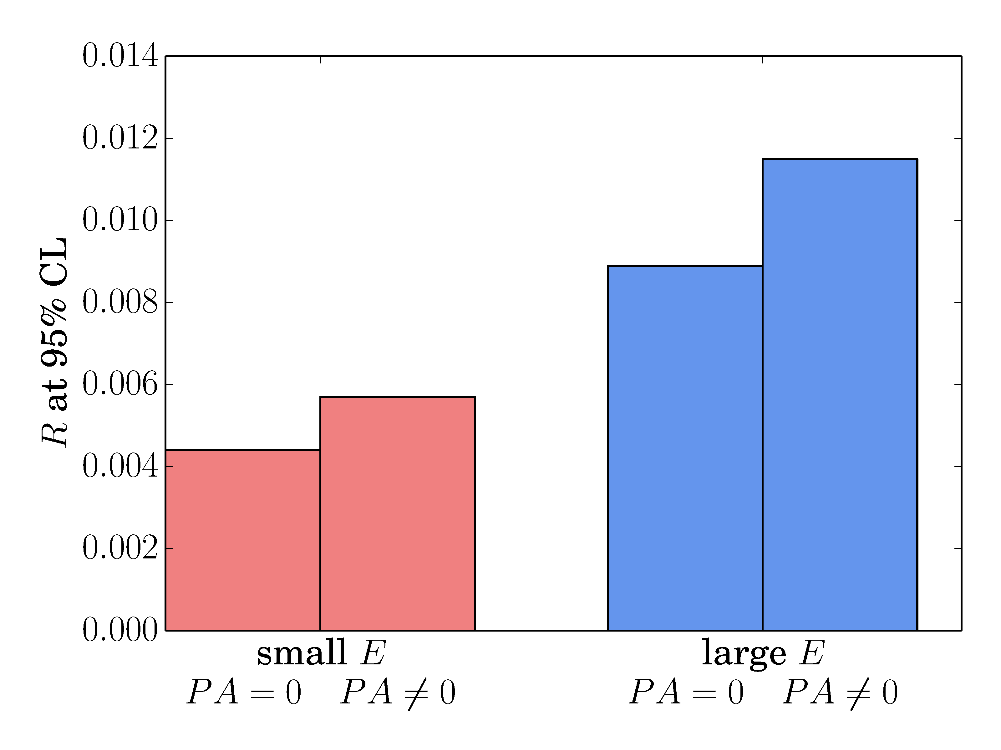
Figure 3: Theoretical upper bounds on $R$. Predictions with (without) $1/N_{c}$ counting are labeled “small $E$” (“large $E$”). To visualize the contribution from exchange diagrams, we also show the result for $PA=0$. The case $PA\neq 0$ is based on the estimate in Eq. (40).

	with $1/N_{c}$		without $1/N_{c}$
	$PA=0$	$PA\neq 0$	$PA=0$	$PA\neq 0$
$|E_{KK}/T^{\mathrm{fac}}|\;\;{\leq}$	1.5		2.6
$R\;\;{\leq}$	0.004	0.006	0.009	0.011

Table 1: $95\%$ C.L. upper limits ($\Delta\chi^{2}=3.84$), with or without $1/N_{c}$ input for $C$ and $E$.

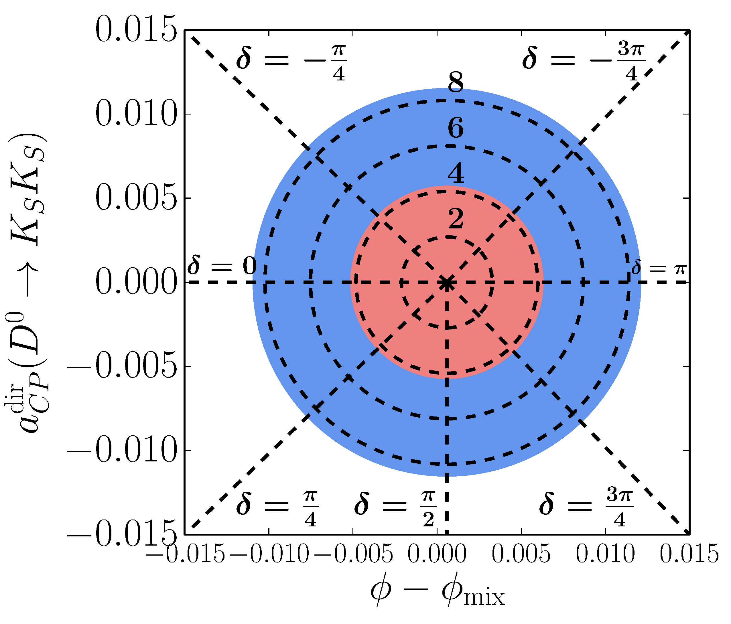
Figure 4: Correlation of direct and mixing-induced CPV for $D^{0}\rightarrow K_{S}K_{S}$ from Eqs. (23) to (25). The one-dimensional $95\%$ C.L. ($\Delta\chi^{2}=3.84$) upper limits on $a_{CP}^{\mathrm{dir}}(D^{0}\rightarrow K_{S}K_{S})$ and $\phi-\phi_{\mathrm{mix}}$ are shown in blue. If in addition $1/N_{c}$ counting is applied to the topological amplitudes $C$ and $E$, the allowed region shrinks to the red area. The black dashed lines show the radii which are obtained when setting $|2E_{KK}+PA|/{2.52\cdot 10^{-6}\,\mbox{GeV}}$ to the annotated values. The chosen reference value is the typical size of a factorized tree amplitude in $D$ decays, $T^{\mathrm{fac}}=2.52\cdot 10^{-6}$ GeV. Further, for the black dashed lines $\mathcal{B}(D^{0}\rightarrow K_{S}K_{S})=0.17\cdot 10^{-3}$ is used. The circle is centered at $(-\mathrm{Im}(\lambda_{b})/\lambda_{sd},0)=(6\cdot 10^{-4},0)$.

Fig. 4 condenses the main results of this paper into a single plot: the radial lines correspond to fixed values of the strong phase $\delta$ in Eqs. (23) and (24) in the $\phi-\phi_{\mathrm{mix}}$–$a_{CP}^{\mathrm{dir}}$ plane. The red and blue discs show the allowed regions for the two considered scenarios. Note that our bounds depend on branching ratio measurements only and do not involve correlations to other CP asymmetries. The black circles correspond to different values of $|2E_{KK}+PA|$ in Eq. (22). Future data on $\phi-\phi_{\mathrm{mix}}$ and $a_{CP}^{\mathrm{dir}}$ will allow us to determine $\delta$ and $R$. The experimental value of $R$ can then be confronted with the upper limits in Table 1 to probe the color counting in $E_{KK}$ and our estimate of $PA$. New physics will mimic a dynamical enhancement of $PA$. In case an anomalously large value of $R$ will be found, one can proceed in the following way to discriminate between different explanations:

• Several CP asymmetries involve $PA$, but do not grow with $|E|$. For example,

  $$a_{CP}^{\mathrm{dir}}(D^{0}\rightarrow K^{+}K^{-}),\,a_{CP}^{\mathrm{dir}}(D^{0}\rightarrow\pi^{+}\pi^{-}),$$

  $$a_{CP}^{\mathrm{dir}}(D^{0}\rightarrow\pi^{0}\pi^{0})\,,$$ (46)

  all depend on $P+PA$ and are expected to be enhanced with $PA$ as well, unless the increase is compensated by $-P$. But in this case instead

  $$a_{CP}^{\mathrm{dir}}(D^{+}\rightarrow K_{S}K^{+}),a_{CP}^{\mathrm{dir}}(D_{s}^{+}\rightarrow K_{S}\pi^{+}),$$

  $$a_{CP}^{\mathrm{dir}}(D_{s}^{+}\rightarrow K^{+}\pi^{0})\,,$$ (47)

  which involve $P$ rather than $P+PA$, become large. Thus a breakdown of color counting in $E_{KK}$ can be distinguished from an enhanced $PA$.

• $PA$ can be enhanced by QCD dynamics or by new physics. In the first case the CP asymmetries in Eqs. (46) and (47) will still obey the sum rules of Ref. Müller et al. (2015b). New physics will violate these sum rules if it couples differently to down and strange quarks.

We close this section by comparing our result with other estimates of $a_{CP}^{\mathrm{dir}}(D^{0}\rightarrow K_{S}K_{S})$ in the literature. Using generic SU(3)_F counting Ref. Brod et al. (2012) quotes

$$|a_{CP}^{\mathrm{dir}}(D^{0}\rightarrow K_{S}K_{S})|\lesssim\frac{2|V_{cb}V_{ub}|}{\varepsilon|V_{cs}V_{us}|}\sim 0.6\%\,,$$ (48)

where $\varepsilon$ quantifies SU(3)_F breaking. Our result in Table 1 agrees with this estimate. However, if the possibility of a large, $1/N_{c}$-unsuppressed $|E_{KK}|$ is realized in nature, $|a_{CP}^{\mathrm{dir}}|$ can be twice as large.

Ref. Hiller et al. (2013) relates $a_{CP}^{\mathrm{dir}}(D^{0}\rightarrow K_{S}K_{S})$ to $\Delta a_{CP}^{\mathrm{dir}}\equiv a_{CP}^{\mathrm{dir}}(K^{+}K^{-})-a_{CP}^{\mathrm{dir}}(\pi^{+}\pi^{-})$. With present data this relation reads

$$|a_{CP}^{\mathrm{dir}}|\lesssim\frac{3}{2}\times\Delta a_{CP}^{\mathrm{dir}}=0.4\%\,.$$ (49)

This estimate assumes that two matrix elements corresponding to different SU(3)_F representations are similar in magnitude. We remark that there is no strict correlation between $a_{CP}^{\mathrm{dir}}(D^{0}\rightarrow K_{S}K_{S})$ and $\Delta a_{CP}^{\mathrm{dir}}$, because the two quantities involve different topological amplitudes.

VI Conclusions

We have studied the direct and mixing-induced CP asymmetries in $D^{0}\to K_{S}K_{S}$ in the Standard Model. The allowed region for the corresponding two quantities $a_{CP}^{\mathrm{dir}}$ and $\phi-\phi^{\mathrm{mix}}$ is a disc whose radius can be calculated in terms of the exchange amplitude $E_{KK}$ and the penguin annihilation amplitude $PA$. We estimate $PA/E_{KK}$ with a perturbative calculation and obtain $E_{KK}$ from a global fit to $D$ branching fractions as described in Ref. Müller et al. (2015a). We find

$$|a_{CP}^{\mathrm{dir}}| \leq 1.1\%\quad(95\%\,\mathrm{C.L.})\,,$$ (50)

$$|\phi-\phi_{\mathrm{mix}}+\mathrm{Im}\frac{\lambda_{b}}{\lambda_{sd}}| \leq 1.1\%\quad(95\%\,\mathrm{C.L.})\,.$$ (51)

A simultaneous measurement of $a_{CP}^{\mathrm{dir}}$ and $\phi-\phi_{\mathrm{mix}}$ will determine $|2E_{KK}+PA|$. A violation of the bound

$$\sqrt{a_{CP}^{\mathrm{dir}}{}^{2}+\left(\phi-\phi_{\mathrm{mix}}+\mathrm{Im}{\frac{\lambda_{b}}{\lambda_{sd}}}\right)^{2}}\leq 1.1\%$$

will point to an anomalously enhanced $PA$. In this case other CP asymmetries will also be enhanced.

Note added in Proof: The authors of Ref. Brod et al. (2012) have informed us that they agree with our expression Eq. (41). The apparent difference is due to a typo in Eq. (13) of Ref. Brod et al. (2012). By comparing our numerical codes we could trace our numerical differences back to the “$i\varepsilon$ problem” mentioned at the end of Sec. IV.