Combining spectroscopic and photometric surveys using angular cross-correlations III: Galaxy bias and stochastisity

Abstract

In the first paper of this series, we studied the effect of baryon acoustic oscillations (BAO), redshift space distortions (RSD) and weak lensing (WL) on measurements of angular cross-correlations in narrow redshift bins. Paper-II presented a multitracer forecast as Figures of Merit (FoM), combining a photometric and spectroscopic stage-IV survey. The uncertainties from galaxy bias, the way light traces mass, is an important ingredient in the forecast. Fixing the bias would increase our FoM equivalent to 3.3 times larger area for the combined constraints. This paper focus on how the modelling of bias affect these results. In the combined forecast, lensing both help and benefit from the improved bias measurements in overlapping surveys after marginalizing over the cosmological parameters. Adding a second lens population in counts-shear does not have a large impact on bias error, but removing all counts-shear information increases the bias error in a significant way. We also discuss the relative impact of WL, magnification, RSD and BAO, and how results change as a function of bias amplitude, photo-z error and sample density. By default we use one bias parameter per bin (with 72 narrow bins), but we show that the results do not change much when we use other parameterizations, with at least 3 parameters in total. Bias stochasticity, even when added as one new free parameter per bin, only produce moderate decrease in the FoM. In general, we find that the degradation in the figure of merit caused by the uncertainties in the knowledge of bias is significantly smaller for overlapping surveys.

1 Introduction

The late time expansion of the Universe can be measured through various probes, including super novas (Riess et al., 1998; Perlmutter et al., 1999), the cosmic microwave background (CMB) (Planck Collaboration et al., 2015), weak lensing shear (Heymans et al., 2013) and galaxy clustering (Anderson et al., 2014). Galaxy clustering is assumed and measured to directly trace the underlying dark matter distribution (Kaiser, 1984; Bardeen et al., 1986), but require measuring the galaxy bias. The weak gravitational lensing directly probe the mass. However, the lensing kernel is broad, which reduce its ability to measure the growth.

Weak lensing (WL) survey relies on averaging a large sample of galaxies, which is only possible in photometric surveys with photo-z techniques. Ongoing surveys include DES(The Dark Energy Survey Collaboration, 2005) and KiDS(de Jong et al., 2013), while Euclid(Laureijs et al., 2011) and LSST(Ivezic et al., 2008) are next generation WL surveys. The galaxy clustering relies on accurate redshift to measure the BAO peak position and the radial clustering. Past and ongoing redshift surveys include VVDS (Le Fèvre et al., 2013), VIPERS (de la Torre et al., 2013) and WiggleZ (Contreras et al., 2013), while DESI (Levi et al., 2013) is expected to start in 2018.

The galaxy clustering and weak lensing are complimentary, probing different parameter degeneracies (Simpson et al., 2013), being subject to different experimental difficulties and astrophysical biases (Weinberg et al., 2013). How should photometric and spectroscopic optimally be combined? Several groups have investigate the benefit of overlapping surveys with varying conclusions (see paper-II) (Bernstein & Cai, 2011; Gaztañaga et al., 2012; Cai & Bernstein, 2012; Kirk et al., 2013; Font-Ribera et al., 2014; de Putter, Doré & Takada, 2013). Our three article series investigates the combined constraints, focusing on the same-sky benefit. In Eriksen & Gaztanaga (2014b) (from now on paper-I) we studied the algorithm and modelling of cross-correlations in narrow redshift bins. Eriksen & Gaztanaga (2015) (from now on paper-II) presented the forecast, while Eriksen & Gaztanaga (2014a) (from now on EG14a) companion paper elaborated on the same-sky benefit. This paper (paper-III) investigate the role of the galaxy bias and stochasticity.

While the galaxy and dark matter distribution is related, the exact relation depends on galaxy formation (Press & Schechter, 1974), galaxy evolution (Nusser & Davis, 1994; Fry, 1996; Tegmark & Peebles, 1998; Blanton et al., 2000) and selection effects. For constraining cosmology with galaxy distributions, we need to model galaxy bias and marginalize over uncertainties in the modelling. To reduce requirements on modelling bias, we can constrain cosmology from the excess of galaxy pairs with 150 Mpc separation, the BAO peak (Eisenstein et al., 2007; Eisenstein, Seo & White, 2007; Anderson et al., 2012). In these papers, constraints from galaxy clustering and galaxy-shear cross-correlations use the full correlation function, which require modelling the galaxy bias (Shoji, Jeong & Komatsu, 2009). This improve the parameter constraints, but the bias becomes an important part of the forecast and is therefore studied here in detail.

Overlapping galaxy surveys allows directly cross-correlation the galaxy samples. Additionally, the sample variance reduce through both galaxy populations tracing the same matter fluctuations (McDonald & Seljak, 2009). Paper-II showed that both effects contribute about equal to the combined constraints and EG14a stressed the importance of the covariance between the spectroscopic and photometric sample. This paper also investigate the additional correlations and the covariance from overlapping volumes, but present the forecasted bias error. In particular, we focus on the counts-shear cross-correlations, since the contribution was largely independent on including lenses from one or both surveys.

The HOD model (Scoccimarro et al., 2001; Zheng et al., 2005; Coupon et al., 2012; Cacciato et al., 2013) predicts the galaxy bias from physical assumptions on how galaxies occupy dense regions, which can be implemented in simulations and tested against real data. The fiducial bias is motivated by a simple HOD model that shows a scale-independent and linear bias at large scales (Gaztañaga et al., 2012). While the bias evolution in a linear model can be parameterized with a few parameters, the fiducial parameterization use one parameter for each redshift bin. Section 3 therefore compare the one-bias-per-bin forecast with a model using a linear interpolation between pivot points.

The fiducial bias model, $\delta_{g}=b(z,k)\delta_{m}$, relate linearly and deterministic the galaxy ($\delta_{g}$) and matter ($\delta_{m}$) overdensities. In reality, the relation at small scales include at stochastic component (Seljak & Warren, 2004). The stochastic component change the auto-correlation of galaxy counts and cancelling in the counts-shear cross-correlations. While the linear scale included in the forecast avoid the bias stochasticity, we study the impact using a simple model (see subsections 3.3, 3.4). In addition to reducing the signal-to-noise, one need to marginalize over the bias stochasticity model parameters. The overlapping surveys is of particular interest, since the overlap can provide additional constraints to these parameters.

This paper is organized in the following manner. Section 2 presents the forecast assumptions, bias derivative formula, fiducial errors and how counts-shear and the sample variance cancellation contribute to the bias error. Then section 3 looks at bias priors, bias parameterization and tests the impact of a stochastic bias. Appendix A study how shifting the bias amplitude change the forecast and the relative RSD, BAO and WL contributions. Finally appendix B study how the galaxy density and redshift uncertainties change the bias errors.

2 The bias constraints

2.1 Forecast assumptions and notation

Parameter	Photometric (F)	Spectroscopic (B)
Area [sq.deg.]	14,000	14,000
Magnitude limit	$i_{AB}<24.1$	$i_{AB}<22.5$
Redshift range	$0.1<z<1.5$	$0.1<z<1.25$
Redshift uncertainty	0.05(1+z)	0.001(1+z)
z Bin width	0.07(1+z)	0.01(1+z)
Number of bins	12	71
Density [gal/arcmin2]	6.5	0.4

Table 1: Parameters describing the assumed photometric and spectroscopic stage-IV surveys in the forecast. See paper-II and EG14a for further details.

Paper-I described the formalism for galaxy clustering, RSD and weak lensing in 2D correlations. In paper-II we presented the Fisher formalism, notation, forecast assumptions and Figures of Merit (FoM). This subsection include, to improve readability, the central forecast setup and notation. The reader is referred to paper-II for a full description.

The forecast define a photometric(F/Faint) and a spectroscopic(B/Bright) stage-IV survey (Albrecht et al., 2006). Table 1 summarize the most important parameters and the forecast use Fisher matrices to estimate the bias errors and FoMs. The fiducial bias redshift evolution is given by

$$b_{F}(z) =1.2+0.4(z-0.5)$$ (1)

$$b_{B}(z) =2.0+2.0(z-0.5)$$ (2)

while the default bias parameterization use one parameter per redshift bin and population. The observables included are auto- and cross-correlations between galaxy counts ($\delta$) and shear ($\gamma$). The redshift space distortions (RSD) and radial information in the galaxy sample is measured by using narrow redshift bins for the spectroscopic sample (Nock, Percival & Ross, 2010; Asorey et al., 2012; Di Dio et al., 2013; Asorey, Crocce & Gaztañaga, 2014).

These papers focus on the benefit of combining spectroscopic and photometric surveys and the notation FxB is short for F and B being overlapping surveys on the sky, while F+B means non-overlapping surveys. The default forecast include both galaxy counts and shear (All), but some result only include galaxy counts (Counts). The Figure of Merit (FoM) is defined by

$$\text{FoM}=\frac{1}{\sqrt{\det(S)}}$$ (3)

where $S$ is a subspace of parameter the Fisher forecasted covariance matrix. For $\text{FoM}_{\text{DETF}}$, the Dark Energy Task Force (DETF) FoM, then $S=[w_{0},wa]$. The $\text{FoM}_{\gamma}$ is the inverse error of $\gamma$, so that the covariance subspace (S) only include $\gamma$. For $\text{FoM}_{w\gamma}$ then S includes $w_{0}$, $w_{a}$, $\gamma$ and measure if a probe can constrain the combined expansion and growth history. Unless explicitly stated, the FoMs and bias errors marginalize over $w_{0},w_{a},h,n_{s},\Omega_{m},\Omega_{b},\Omega_{DE},\sigma_{8},\gamma$. Planck priorsis always included.

2.2 Derivative of the galaxy bias

The default bias parameterization is one parameter per redshift bin and galaxy population. This subsection presents a formula for the derivative of the 2D correlation with the bias when including photo-z, RSD, magnification and multiple galaxy populations.

Photo-z uncertainties cause overdensities with origin at one redshift, to be observed at another redshift. One can express the observed fluctuations as a linear contribution from different redshifts. The galaxy bias evolve with redshift and the observed overdensity is a convolution of the bias and redshift selection function (see paper-I). For the bias derivative, the parameters can either be defined as the true bias or an effective bias after including the photo-z effect. These papers (paper-II, paper-III, EG14a), use the true bias as nuisance parameters.

The photo-z effect in 2D correlations can be approximated by the transition matrices (Gaztañaga et al., 2012). Let $\bm{\mathsf{C}}$ be a matrix of 2D correlation predictions in top-hat bins. The observed correlations $\bm{\mathsf{\tilde{C}}}$ including photo-z effects can be written

$$\tilde{C}_{ij}=\sum_{mn}r_{im}r_{jn}C_{mn}$$ (4)

where $r$ is a transition matrix. The matrix element $r_{ij}$ is the fraction of a fluctuation in bin $i$ which originates from bin $j$. Summing over the transition matrix elements is effectively a low resolution integral over the redshift selection function. In Eq.4 the first and second transition matrix respectively corresponds to the first and second index of C. When generalizing the formula to several populations and overdensity types (counts, shear), the two transition matrices (r) will differ. While the transition matrices for the Bright and Faint populations can be different, they are in these papers considered equal for shear and galaxy counts for each population (Faint, Bright).

The transition matrix leads naturally to an expression for the bias derivative. Let $\tilde{C}_{ij}^{AB}$ be the observed correlation of A and B, in respectively redshift bin $i$ and $j$. Define further $b_{y}^{X}$ to be the bias of overdensity type X in redshift bin y. The derivative of the observed correlation with respect to the bias is then

$$\frac{\partial\tilde{C}_{ij}^{AB}}{\partial b^{X}_{y}}\ =\sum_{m,n}\left[r_{iy}^{X}r_{jn}^{B}C_{yn}^{\rho B}+\ r_{im}^{A}r_{jy}^{X}C_{my}^{A\rho}\right]$$ (5)

where $C^{\rho X}$ is the cross-correlation of dark matter in real space and one overdensity of type $X$. These papers only include the parameter $b^{X}$ for galaxy counts, but Eq.5 can in general be used for shear intrinsic alignments, clustering of galaxy sizes or clustering of magnitudes.

Galaxy clustering, redshift space distortions, cosmic magnification and other minor effects, all contribute to the galaxy counts overdensities. Among these effects, only the galaxy clustering in real space depends on the bias. Most importantly, the RSD contribution depends on the velocity introduced by the underlying matter fluctuations and is independent of the galaxy bias. A central idea in these papers is to measure RSD in 2D correlation functions by using narrow redshift bins. Since the derivative should only consider parts of the correlations caused by the galaxy clustering, Eq.5 includes the cross-correlation between matter and the observable. When using the algorithm outlined in paper-I, then estimating these cross-correlations does not require redoing the full calculations, but can be performed faster by reusing intermediate results in the calculations.

2.3 Bias errors in the fiducial configuration.

Figure 1: The relative error on galaxy bias, marginalized over other cosmological parameters and including Planck priors. The four lines corresponds to the Bright and Faint populations, for overlapping (x) and non-overlapping (+) surveys. Points corresponds to errors measured using one bias parameter for each bin. On the x-axis is the mean for each the corresponding redshift bin. For the bright sample the bins are thinner, which results in more points. In the top panel the measurements only includes galaxy counts, while the lower panel also includes shear.

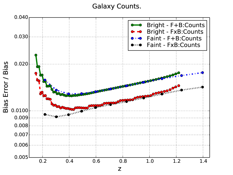
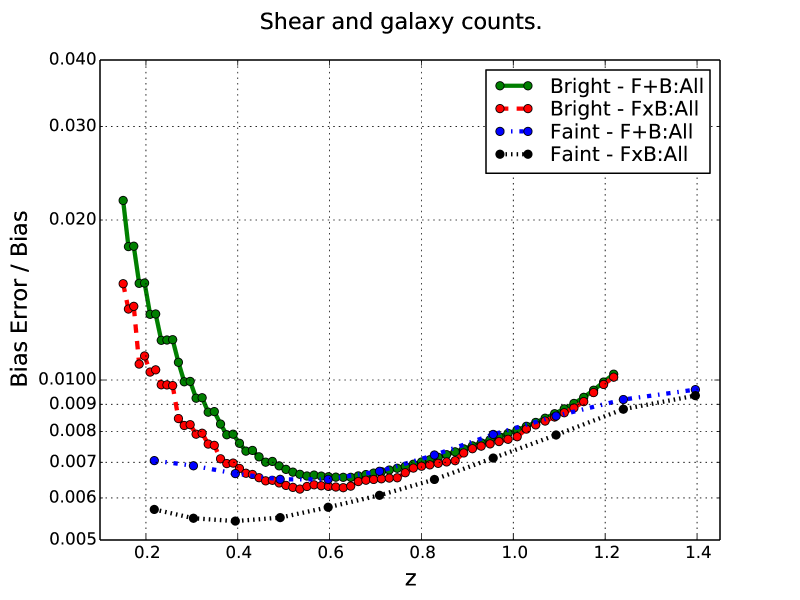
Fig.1 shows the estimated bias errors relative to the fiducial bias. While the forecast include redshift bins from $z=0.1$ for both galaxy populations, the first bins has little constraining power. At low redshifts the bias error diverges and we therefore show only the error for $z<0.2$. For both the exact calculations and the Limber approximation, the main contribution to an auto-correlation signal is the scale $k=(l+0.1)/\chi(z)$ and lower redshifts enter into non-linear scales for smaller l. We remove in the forecast correlations which enters into the non-linear regime (see paper-II) and this leads to worse constrains at low redshifts. Also, the bias is parameterized using the underlying/true bias (see subsection 2.2). Even if a redshift bin is excluded at a particular scale (l-value), the bias parameter enters in cross-correlations measured in nearby bins from the photo-z dispersion.

Lines in Fig.1 show the relative bias error. The top panel only include galaxy counts in the forecast. For both populations the estimated bias error are similar for the Bright and Faint population, except for overlapping surveys at low redshifts where magnification contribute stronger to the Faint bias constraints. For galaxy clustering the relative bias constraints are very similar for both populations, but becomes different if fixing the cosmological parameters (not shown). Overlapping galaxy surveys significantly lower the bias and benefit the two populations about equally much. In the lower panel also counts-shear and shear-shear correlations are included in the forecast. Lensing both directly measuring bias through the counts-shear observables, but also indirectly through better constraining cosmological parameters, which are discussed respectively in subsection 2.5 and 2.4.

Figure 2: The same-sky benefit on measuring the galaxy bias. Lines show the non-overlapping/overlapping samples bias error ratio. Each line plots the bias error in non-overlapping samples over overlapping samples. For ratios over unity overlapping samples are beneficial in measuring the bias. The thin vertical lines mark the edges of the Faint redshift bins.

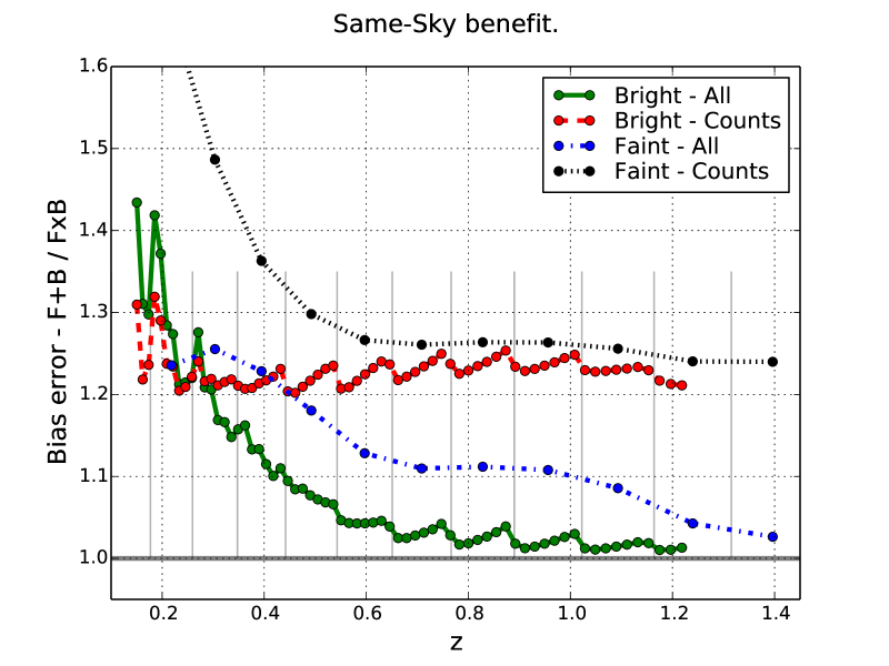
Fig. 2 shows directly the F+B/FxB bias error ratios, which is the same-sky benefit. For both the Bright and Faint bias, with and without shear, overlapping surveys leads to better bias constraints. Including the shear signal reduce the benefit of overlapping samples compared to only galaxy counts. This trend was previously seen in the forecast (paper-II, Table 4 and 5) and is here shown directly for the bias error. When including lensing, both the galaxy clustering and counts-shear observables can measure the bias. While this improve the bias measurements and forecast, the multiple ways of constraining the bias lower the effect of overlapping Bright and Faint galaxy counts. The Bright bias error also depend on which Faint redshift bin the Bright bin overlap. This cause a small drop in the Bright ratios at the edges of a Faint bin, which are marked with vertical lines.

2.4 Correlation between cosmology and bias

Figure 3: Effect of the covariance between cosmological and bias parameters. The lines show the Faint bias error ratios for free/fixed cosmological parameters. On the x-axis is the redshift. Two lines (FxB:All, F+B:All) plots the ratio including galaxy counts and shear, while the other two (FxB:Counts, F+B:Counts) only include galaxy counts.

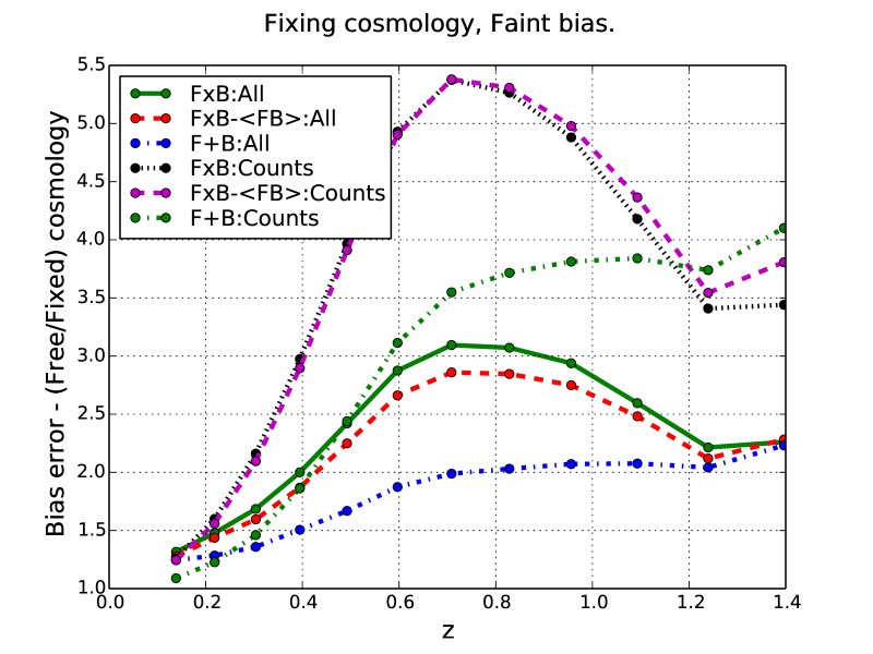
The cosmological constraints from galaxy clustering require marginalizing over uncertainty in the galaxy bias modelling. Fixing the galaxy bias would increase the $\text{FoM}_{w\gamma}$ forecast for FxB:All equivalent to a 3.3 larger survey area. The cosmology constraints depend both on measuring the bias and the lowest possible covariance between the cosmological and bias/nuisance parameters (see Eriksen & Gaztanaga (2014a)). In studying the bias error, one should account for this covariance. This subsection focus on how marginalizing/fixing cosmological parameters would affect conclusions on overlapping surveys and the importance of weak lensing.

Fig. 3 shows the Faint free/fixed cosmology bias error ratio. These ratios should always be above unity, since marginalizing over cosmology increase the bias errors. To limit the discussion, the figure and discussion are for brevity restricted to only the Faint bias. While the magnitude and exact details differs, the main conclusions are similar for the Bright sample. In this figure, the FxB ratios peaks around $z=0.7$, which results from a peak in the Faint galaxy density and disappear a very high galaxy density (not shown). Around $z=0.7$, the FxB:Counts(F+B:Counts) ratio is 5.3(3.1) and this change in bias error corresponds to effectively 28(9) times larger area. In comparison, FxB:All versus F+B:All only increase $\text{FoM}_{w\gamma}$ for FxB:All equivalent to 50% larger area. When studying how improved bias measurements impact overlapping surveys, one need to account for the covariance between cosmological and bias parameters. Results without covariance will tend to underestimate the benefit of overlapping surveys.

Figure 4: Effect of limiting the redshift separation in the cross-correlations. Errors are estimated for FxB:All. The top panel shows the bias errors, while the bottom panel shows the free/fixed cosmology bias error ratio. On the x-axis is the maximum distance between the mean of the two redshift bins in a correlation ($\Delta Z_{\text{Max}}$).

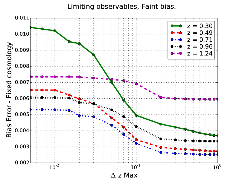
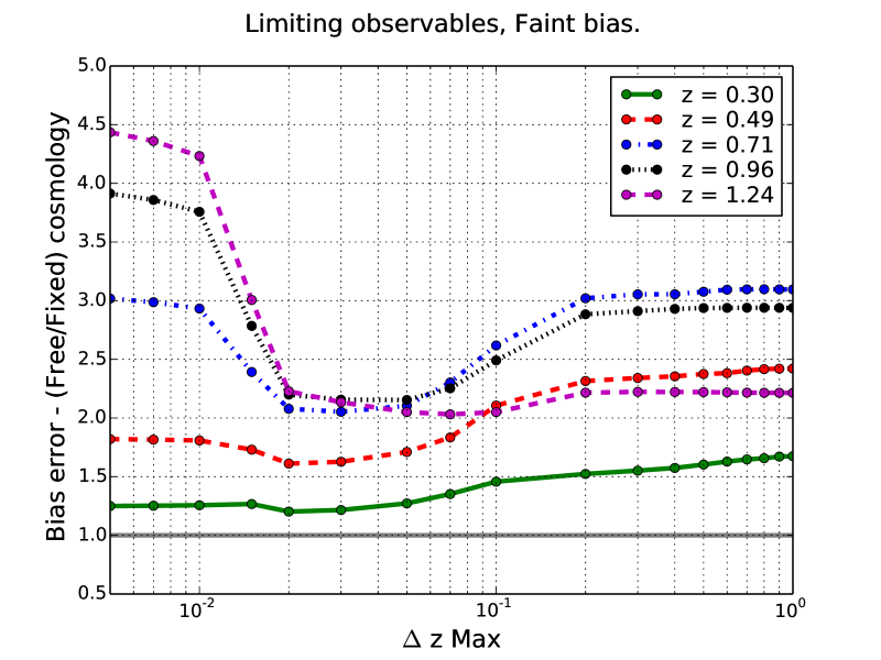
Fig.4 shows results when varying $\Delta Z_{\text{Max}}$. The $\Delta Z_{\text{Max}}$ requirement limit which correlations are included in the forecast. It was introduced in paper-II and limit the forecast to only include cross-correlations with ($|z_{j}-z_{i}|\leq\Delta Z_{\text{Max}}$), where $z_{i}$ and $z_{j}$ are the mean redshifts for the two overdensities in the cross-correlation. The auto-correlations are always included. For $0.0<\Delta Z_{\text{Max}}<0.1$ the forecast also include Bright-Faint galaxy counts cross-correlations, while $0.01<\Delta Z_{\text{Max}}\lesssim 0.03$ include the important radial (between redshift) Bright-Bright cross-correlations. The counts-shear correlations are first important at larger $\Delta Z_{\text{Max}}$. For further examples of usage, see paper-II.

The top panel (Fig. 4) show the estimated Faint bias error, fixing the cosmological parameters. When increasing $\Delta Z_{\text{Max}}$, the Bright-Faint cross-correlations are included and the bias error decline steadily. At higher $\Delta Z_{\text{Max}}$ the counts-shear only leads to very small improvements in the bias error. In the bottom panels are bias error ratios for free/fixed cosmology. For $0.01<\Delta Z_{\text{Max}}<0.02$ the forecast includes Bright-Bright radial cross-correlations, which measure cosmological parameters and the ratio drops. At high $\Delta Z_{\text{Max}}$ the observables include the counts-shear cross-correlation. This signal increase the correlation between cosmology and bias parameters, which results in the ratios increasing.

2.5 Counts-shear cross-correlations

Figure 5: The improvement from counts-shear cross-correlations in the Faint bias measurements. Lines are the bias error ratios between FxB:All without some counts-shear cross-correlations and FxB:All. In FxB-$\left<\delta_{F}\gamma_{F}\right>$[FxB-$\left<\delta_{B}\gamma_{F}\right>$] all correlations are included, except counts-shear cross-correlations within the Faint[Bright] sample. In FxB-$\left<\delta\>\gamma\right>$ all the counts-shear cross-correlations are removed.

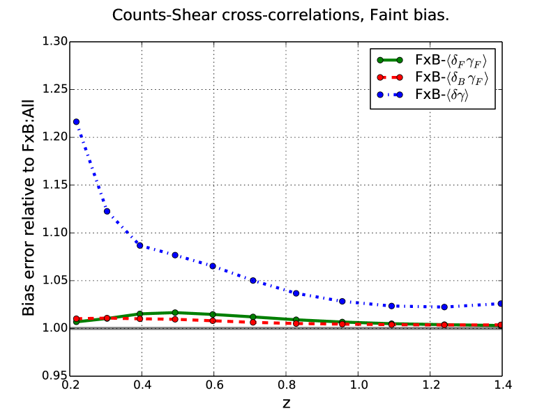
In paper-II we studied how different counts-shear cross-correlations contribute to the cosmological forecast. Overlapping surveys make it possible to cross-correlate spectroscopic (Bright) galaxy counts with galaxy shear from a photometric (Faint) survey. For a photometric survey, one can also cross-correlate the counts and shear, both measured from the photometric survey. These two counts-shear cross-correlation types contribute about equal to the cosmological parameter forecast(see paper-II, table 4 and 5). Removing either counts-shear cross-correlations only lead to a small decrease in the different figures of merit. However, the constraints drop significantly when removing all counts-shear cross-correlations.

A contributing factor is the bias constraints from the cross-correlations. In Fig.5 are the error ratios between FxB:All without some counts-shear cross-correlations and FxB:All. For FxB-$\left<\delta_{F}\gamma_{F}\right>$ and FxB-$\left<\delta_{B}\gamma_{F}\right>$, we respectively remove the cross-correlations of Faint and Bright galaxy counts with the Faint shear. The change is small for removing either Bright or Faint lenses, typically less than 1%. On the other hand, when removing all counts-shear cross-correlations (FxB-$\left<\delta\>\gamma\right>$) the bias error change significantly. The Bright bias follow a similar trend (not shown), except counts-shear contributing less below $z=0.4$.

This trend follows from a high correlation between the count-shear signal in overlapping lens bins. Using the covariance for a Gaussian field (see paper-I), the correlation coefficient between counts-shear using two galaxy populations as lenses is

$$r[\left<\delta_{B}\gamma\right>,\left<\delta_{F}\gamma\right>] \equiv\frac{\text{Cov}\left(\left<\delta_{B}\gamma\right>,\left<\delta_{F}\gamma\right>\right)}{\sqrt{\text{Var}\left(\left<\delta_{B}\gamma\right>\right)\text{Var}\left(\left<\delta_{F}\gamma\right>\right)}}$$ (6)

$$\approx\frac{\left<\delta_{B}\delta_{F}\right>}{\sqrt{\left<\delta_{B}\delta_{B}\right>\left<\delta_{F}\delta_{F}\right>}}$$ (7)

where $\delta_{B}$($\delta_{F}$) is the Bright(Faint) galaxy counts and $\gamma$ is the galaxy shear overdensities. To simplify the notation, $\left<\right>$ denote a Cl cross-correlation and we suppress the redshift bin index. From numerical tests (not shown), the terms including galaxy counts dominate. Unlike for the galaxy counts, the RSD contribution is negligible for the counts-shear correlations and the signal is effecively linear with the lens bias. The strong correlation is therefore not introducing sample variance cancellation. Instead it reduce the value of using two different galaxy populations as lenses.

2.6 Sample variance cancellation

Figure 6: Effect of overlapping volumes. The plots show the bias error ratios of F+B:All and FxB-$\left<\text{FB}\right>$ with respect to FxB:All. The F+B:All combine the populations over separate volumes, while FxB-$\left<\text{FB}\right>$ is overlapping surveys without cross-correlating the observable. These definitions discriminate between constraints from the covariance and additional cross-correlations.

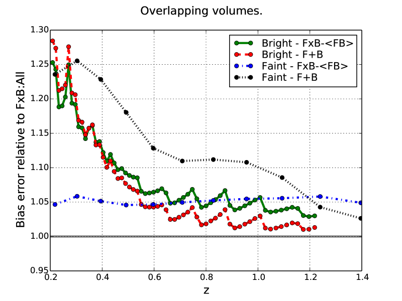
Overlapping surveys gain from both additional cross-correlations and sample variance cancellation. Even without including the additional observables, two overlapping surveys with free galaxy bias benefit from overlapping skies. The overlapping surveys introduce additional covariance between the observable, which improve the constraints when different observables respond sufficiently different to the same variable (see EG14a). These two effects contribute about equal to the combined forecast (paper-II, table 4 and 5).

Fig. 6 distinguish between the two main effects contribution, the additional cross-correlations and sample variance cancellations, directly in the bias error. Both effects are included in F+B/FxB, while FxB-$\left<\text{FB}\right>$/FxB only show the contribution from sample variance cancellation. These two effects both decrease the Faint bias error, but the additional Bright-Faint cross-correlations contribute most. The Faint/photometric sample has broad redshift uncertainty (see Table 1) and benefit less from RSD and BAO. The Bright-Faint cross-correlations partly recover this information, which makes them suitable for constraining the Faint bias (see paper-I). These correlations are less important for the Bright sample, where the sample variance cancellation is most important. A single Faint redshift bin ($\Delta z=0.07(1+z)$) overlap with multiple Bright bins ($\Delta z=0.01(1+z)$). This introduce a covariance between the Faint bias parameter and each of the Bright bias parameters, which then also indirectly correlate the Bright bias parameters.

2.7 Bias amplitude

The fiducial bias evolution was given in Eq. 2. At redshift zero the fiducial bias for the Bright and Faint populations equals, while the Bright/Faint bias ratio is respectively 1.7 and 2.1 for $z=0.5$ and $z=1$. This section introduce an additional multiplicative amplitude (relative bias amplitude), meaning unity is the fiducial bias.

Figure 7: Effect of the Bright galaxy bias amplitude on the FoMs. On the x-axis is a multiplicative amplitude relative to the fiducial Bright bias. A vertical line ($x=1$) marks the fiducial case. The top, middle and bottom panels respectively show the impact for $\text{FoM}_{w\gamma}$, $\text{FoM}_{\text{DETF}}$ and $\text{FoM}_{\gamma}$.

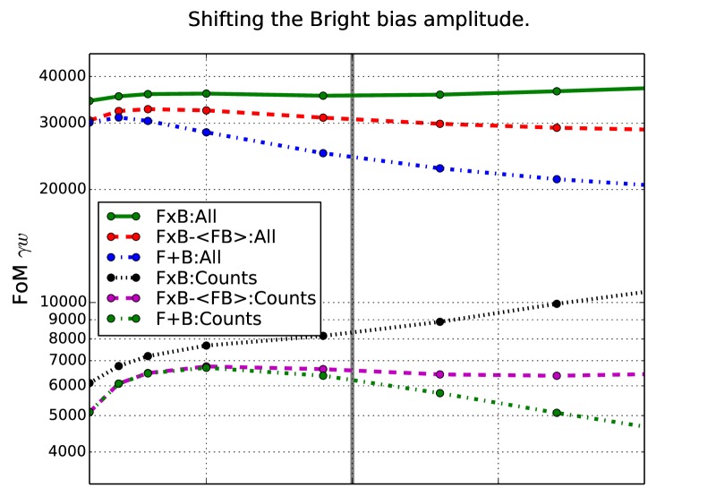
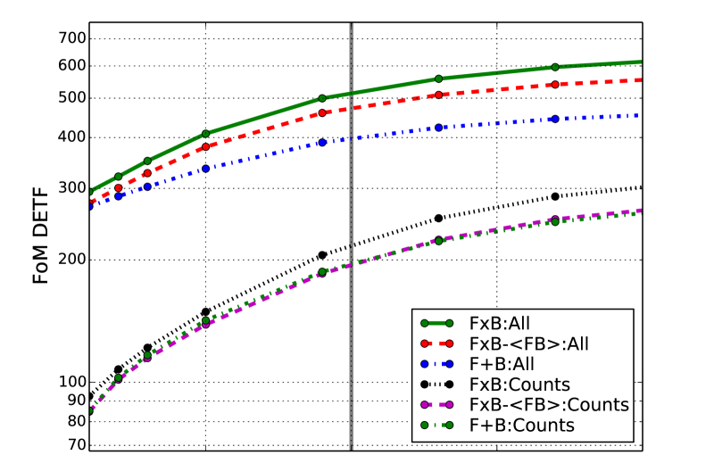
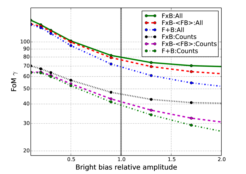
Fig. 7 shows $\text{FoM}_{w\gamma}$, $\text{FoM}_{\text{DETF}}$ and $\text{FoM}_{\gamma}$ for a shifted Bright bias amplitude. In the top panel, the different probes (lines) gain or decline moderately with a shifted bias. $\text{FoM}_{w\gamma}$ combine the expansion and growth history constrains, which are affected differently by the bias amplitude. For $\text{FoM}_{\text{DETF}}$ (middle panel) measuring the expansion history ($w_{0},w_{a}$), the constraints increase with the Bright bias, while the growth constraints in $\text{FoM}_{\gamma}$ decline. This cause the $\text{FoM}_{w\gamma}$ combined constraints to be quite flat. These competing trends cause $\text{FoM}_{w\gamma}$ to change less with the Bright bias amplitude.

The galaxy counts shot-noise is independent of bias and depends inversely on the surface density of galaxies, leading to a higher noise term for the galaxy clustering of the Bright (spectroscopic) sample. Since the auto-correlations are proportional to $b^{2}$, a higher bias increase the signal and therefore reduce the sensitivity to the shot-noise. Doubling the bias corresponds (without RSD) to four times higher density. Without the Bright galaxy shot-noise, the trends change completely, with the ratios being flat for a Bright bias relative amplitude above 0.5. The trend in $\text{FoM}_{\text{DETF}}$ is therefore caused by a higher (lower) bias amplitude lowering (increasing) the impact of shot-noise.

Gravitational infall of galaxies towards matter overdensities along the line of sight introduce an additional redshift, which result in the redshift space distortions (see paper-I). The additional observed overdensity depends only on the matter distribution and is independent of the galaxy clustering and the galaxy bias. The galaxy bias therefore determine the relative strength of the intrinsic clustering and the RSD signal. For a low bias amplitude the RSD signal dominate, while the intrinsic galaxy clustering becomes more important for a high bias. The $\gamma$ constraints ($\text{FoM}_{\gamma}$) are mostly from RSD and therefore decrease with the bias amplitude. This trend also hold when not including the Bright shot-noise.

The lines FxB-$\left<\text{FB}\right>$:All [FxB-$\left<\text{FB}\right>$:Counts] are FxB:All [FxB:Counts] without including the Bright-Faint cross-correlations, but they benefit from overlapping volumes. These lines therefore distinguish between the two sources of FoM improvements. For FxB:All and $\text{FoM}_{w\gamma}$ at the fiducial bias, these effects contribute about equal. The sample variance contribute stronger when including lensing and even when fixing the bias. We attribute this to the overlap introducing a covariance between clustering and lensing observables, which correlates the cosmological parameters later marginalized over. At lower Bright bias amplitudes the sample variance cancellation contribute less for all FoMs (FxB-$\left<\text{FB}\right>$$\approx$ F+B). Without shot-noise (not shown) the overlapping samples still benefit from sample variance cancellations, which means a sufficient density compared to the amplitude is needed to benefit from the two tracers.

Not included are the FoMs when varying the Faint bias amplitude. The Faint sample models a photometric survey with $\sigma_{z}=0.05(1+z)$, which is more suitable for weak lensing than galaxy clustering, since a photo-z above $\sigma_{z}\approx 0.005(1+z)$ erase radial information (Gaztañaga et al., 2012). Compared to the Bright bias (Fig.7), the changes is therefore smaller when shifting the Faint bias. However, unlike the Bright bias, the effect of shot-noise decrease with the Faint bias (not shown). Increasing the Faint bias decrease the bias difference between the populations and this reduce the benefit of using two tracers.

3 Bias priors and modeling

The last section studied the bias errors and the effect of the bias amplitude. This section looks at various aspects of the galaxy bias. The fiducial bias is deterministic, parameterized by one parameter for each bin and include no priors. The first subsection quantify the effect of adding priors on the bias. In the second subsection we compare the cosmological constraints for two different bias parameterizations. In the last subsection we add stochasticity.

3.1 Absolute priors on bias.

Figure 8: The effect of adding priors to the bias parameters. On the x-axis is the prior (error) added independent to each bias parameter and only for one population. The left(right) panels add priors to the Bright(Faint) sample. The top(bottom) panels show the effect of $\text{FoM}_{w\gamma}$($\text{FoM}_{\gamma}$). Lines correspond to the combinations FxB:All, FxB-$\left<\text{FB}\right>$:All, F+B:All, FxB:Counts, FxB-$\left<\text{FB}\right>$:Counts and F+B:Counts.

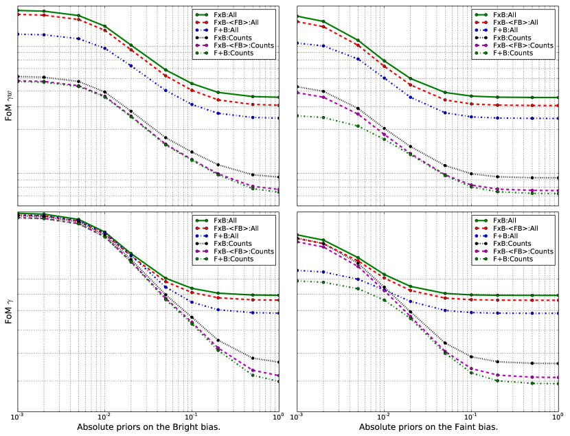
This subsections study how the forecast change when adding uncorrelated priors on the bias. Adding priors give results in between a fixed and free bias. Bias priors from e.g. the 3pt function (Gaztañaga & Scoccimarro, 2005; Gaztañaga et al., 2005; Sefusatti et al., 2006; Frieman & Gaztanaga, 1994; Bel, Hoffmann & Gaztañaga, 2015) or simulations, would usually have covariance between the parameters. However, adding a fixed and uncorrelated prior (flat prior) on each bias parameter simplify the model. Understanding the potential gains and required level of accuracy is important before deciding if the improved constraints justify the required effort. In this subsection, the bias priors is only added to one population.

Fig. 8 shows the forecast when adding priors on either the Bright or Faint bias. Here rows corresponds to the FoMs and columns to which population the bias is added to. The left side of the graph is effectively fixing the bias, while on the right the priors are weak. For FxB:Counts and F+B:Counts, the $\text{FoM}_{w\gamma}$ and $\text{FoM}_{\gamma}$ forecast increase already for very weak Bright priors (0.5). When including lensing (FxB:All and F+B:All), stronger priors is needed, since lensing also constrains the bias. Around absolute priors of ${10}^{-2}$ the constraints flatten and beyond this point increasing bias priors provide no additional benefit.

How does the Bright priors affect the conclusion on overlapping versus non-overlapping galaxy surveys? In the top,left panel stronger priors on the Bright bias increase $\text{FoM}_{w\gamma}$ for all probes with a factor of a few. However, the same-sky ratios (FxB/F+B):All and (FxB/F+B):Counts are respectively close to constant and decrease significantly. Overlapping surveys including shear (All) are therefore equally powerful when knowing the Bright galaxy bias. For overlapping surveys the Bright priors directly improve counts-shear cross-correlations of Bright lenses. The Bright priors additionally lead to stronger constraint on the Faint bias through counts-counts cross-correlations, which again benefits the cross-correlations of Faint counts with shear. For $\text{FoM}_{\gamma}$ all probes, (Fig. 8, bottom left panel), approach the same asymptotic value. The growth constraints are already without priors dominated by redshift space distortions in the Bright sample. Naturally the Bright sample dominates the growth constraints when effectively fixing the Bright bias and this results in no benefit from the overlap (FxB).

The right column (Fig. 8) add priors to the Faint bias. In the top panel ($\text{FoM}_{w\gamma}$), the trend for FxB:All and F+B:All is similar to when adding priors on the Bright bias. The largest difference is for the growth constraints ($\text{FoM}_{\gamma}$) in the bottom panel. For stronger priors F+B:Counts saturates, while FxB:Counts continues improving. We have included FxB-$\left<\text{FB}\right>$, which is FxB without the Bright-Faint cross-correlations. The FxB:Counts and FxB-$\left<\text{FB}\right>$:Counts lines are close for strong Faint priors, which shows the gain comes through sample variance cancellation (overlapping volumes) and not the additional cross-correlations. Finally, one should remember Fig. 8 includes priors on only one population. When fixing the priors, paper-II (table 5 and 6) found less benefit of overlapping surveys.

3.2 Comparing bias parameterizations.

Figure 9: Effect of fixing the galaxy bias for a different number of Bright redshift bins. The $\text{FoM}_{w\gamma}$ ratio is between a fixed and marginalized galaxy bias, with lines corresponding to FxB:All, F+B:All, FxB:Counts, F+B:Counts and B:Counts. On the x-axis is the number of redshift bins in the Bright sample and the vertical line (bins = 72) mark the fiducial number of bins.

Figure 10: Comparison between two different bias parameterizations. The FoM ratios are between a linearly interpolated and the one-parameter-per-bin parameterization of the Bright bias. The Faint bias use one-parameter-per-bin. One the x-axis is the number of interpolation points, which scaled by $\Delta z\propto(1+z)w$ (see text). The lines corresponds to FxB:All, F+B:All, FxB:Counts and F+B:Counts.

Galaxy bias evolve slowly with redshift (Gaztañaga et al., 2012). How many parameters are actually needed to capture the evolution? This series of papers (paper-II, paper-III, EG14a) parameterize the bias by one parameter in each bin and galaxy population. One could instead specify the bias for a few pivot points in redshift and interpolate between them. The potential advantage is reducing the parameter freedom and therefore increasing the statistical errors after marginalizing over the bias. However, including sufficient freedom in the bias parameterization will bias the cosmological constraints (Clerkin et al., 2015). This subsection (and paper) focus only on the statistical errors.

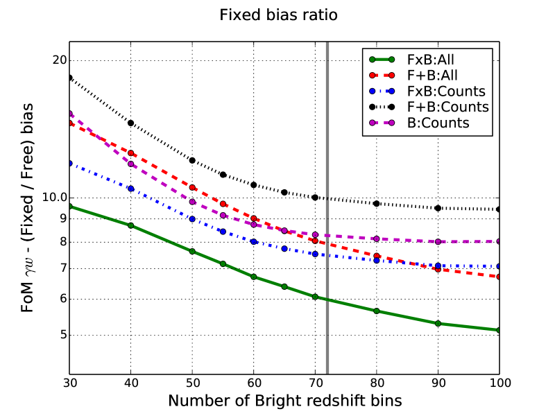
Fig. 9 shows the ratio between Fixed/Free galaxy bias for an increasing number of redshift bins. This partly answer the question if the forecast becomes more or less sensitive when increasing the number of redshift bins. Previously paper-II studied the effect of adding more Bright redshift bins. Here we find that increasing the number of redshift bins is not increasing the sensitivity to bias. On the contrary, the sensitivity to the bias is decreasing with an increasing number of bins. The decrease is driven by the dark energy constraints. Looking at $\text{FoM}_{\gamma}$, the ratios is quite flat, while $\text{FoM}_{w}$ and $\text{FoM}_{\text{DETF}}$ decline (not shown) and result in $\text{FoM}_{w\gamma}$ declining.

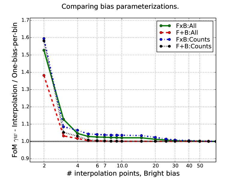
An alternative bias parameterization is linearly interpolating between a bias specified in pivot points (Gaztañaga et al., 2012). Fig. 10 compare $\text{FoM}_{w\gamma}$ when using a linear interpolated and one-bias-per-bin Bright bias parameterization. The distance between bias pivot points scale by $\Delta_{z}\propto(1+z)$, similar to the redshift binning. Earlier, the forecast found $\text{FoM}_{w\gamma}$, $\text{FoM}_{\gamma}$, $\text{FoM}_{w}$ and $\text{FoM}_{\text{DETF}}$ for FxB:All to become 6.0, 2.0, 3.0 and 3.4 times higher when fixing the galaxy bias (see paper-II, table 4 and 5). When only having two Bright bias interpolation points, the $\text{FoM}_{w\gamma}$ forecast is 40-60% higher depending on the probe. For 3 bias points the result is within 10% of the one-bias-per-bin result and the two bias parameterizations fully converge for more interpolation points. The reduction of $\text{FoM}_{w\gamma}$ already occurs for a few interpolation points, which is needed since the bias evolve with redshift. We therefore conclude that using one-bias-per-bin is not leading to unreasonable large degradation in the statistical constraints.

3.3 Stochasticity model

The relation between dark matter and galaxies is on large scale arguably close to deterministic (Gaztañaga et al., 2012). In these papers the fiducial bias model for both galaxy populations are deterministic and linear in mass, meaning

$$\delta_{g}=b\delta_{m}$$ (9)

where $b$ is the galaxy bias and $\delta_{g}$ and $\delta_{m}$ are respectively the galaxy and matter overdensities. A stochastic relation between the matter and galaxy overdensities can be written

$$\delta_{g}=b\delta_{m}+\epsilon$$ (10)

where $\epsilon$ is the random component. Any linear matter dependency in $\epsilon$ would only lead to a redefined bias. More generally both the bias and stochasticity could depend on higher order of the matter fluctuation. These models are beyond the scope of this article.

The resulting power spectrum when including a stochastic component uncorrelated with matter (Eq. 10) is

$$\tilde{P}(z,k)=P(z,k)+A(z,k)$$ (11)

where $A(z,k)$ is an additional contribution to the power spectrum $P(z,k)$. In general this contribution can depend on galaxy population, redshift and scale. By calibrating against simulations, one could try to measure the expected errors, scale and redshift dependence of $A(z,k)$. One should note, such a calibration would require several simulations to assess the impact of cosmology. We instead focus on the direct effect on the auto-correlation

$$C_{ii}=b^{2}\left<\delta_{m},\delta_{m}\right>+\left<\epsilon,\epsilon\right>$$ (12)

for which the stochasticity introduce an additional term $\left<\epsilon,\epsilon\right>$. We assume the stochasticity in different redshift bins are uncorrelated, which leads to unchanged cross-correlations. Environmental effects can introduce correlations of the stochasticity of galaxy populations, but they are for simplicity considered independent. The stochastic component can be modelled by

$$\overline{C}^{xy}=C^{XY}+\delta_{XY}S$$ (13)

where $X$,$Y$ are the galaxy populations and $S$ the additional component. The standard stochasticity function $r$ is the ratio

$$r^{2}\equiv\frac{({\overline{C}_{gm})}^{2}}{\overline{C}_{gg}\overline{C}_{mm}}$$ (14)

where $\overline{C}_{gm}$, $\overline{C}_{gg}$ and $\overline{C}_{mm}$ are respectively the counts-matter, counts-counts and matter-matter correlations when including the bias stochasticity. This ratio (Eq. 14) relates to our definition (Eq. 13) by

$$r^{2}=\frac{C^{2}_{gm}}{(C_{gg}+S)C_{mm}}={\left(1+\frac{S}{C_{gg}}\right)}^{-1}$$ (15)

or alternatively the relation can be written be reversed and written

$$S=C_{gg}(1-r^{-2}).$$ (16)

From Eq.15 and 16, values of $S$ need to be comparable with the auto-correlations to be significant. The no-stochasticity limit is $r=1$ or $S=0$. In addition to simplifying the addition of stochasticity, the term $S$ has similar characteristics as the shot-noise. Results on uncertainties in the stochasticity can therefore be extended to uncertainties of the galaxy counts shot-noise.

3.4 Bias stochasticity

The fiducial galaxy bias in these articles is deterministic. In this subsection we study the impact of introducing bias stochasticity (non-deterministic bias). The last subsection (3.3) introduced a simple redshift and scale independent parameterization of the stochasticity, deviating from the commonly used function $r$. First we study how an increasing stochasticity reduce the signal-to-noise and then how uncertainties in the stochasticity impacts the forecasts.

Figure 11: Effect of increasing galaxy bias stochasticity. The $\text{FoM}_{w\gamma}$ is plotted with the x-axis being the Bright galaxy bias stochasticity parameter S. The fiducial value is $S=0$ where the galaxy bias is deterministic and here no extra nuisance parameters are added to describe the stochasticity. The second/top x-axis is the stochasticity $r$ when assuming $C_{gg}=3\times{10}^{-4}$, which corresponds to a Bright counts-counts auto-correlation at $z=0,l=100$.

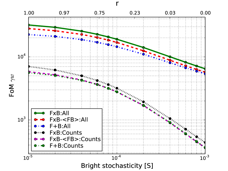
Fig. 11 shows $\text{FoM}_{w\gamma}$ when increasing the galaxy bias stochasticity for the Bright population. The stochasticity variable is fixed, in other words, the stochasticity is assumed known. Since the stochasticity is just noise, it monotonically reduces the figure of merit. The FoMs decrease when the stochastic component (S) comparable to the signal. For the different probes and also $\text{FoM}_{w}$, $\text{FoM}_{\gamma}$ and $\text{FoM}_{\text{DETF}}$ (not shown), the FoMs decrease steadily. The benefit of overlapping surveys (FxB:All/F+B:All) reduce for a higher bias stochasticity. From comparing FxB:All and F+B:All with FxB-$\left<\text{FB}\right>$:All, one see the bias stochasticity reduce the gain from sample variance cancellations. Finally, the equivalent Faint bias stochasticity plots (not included) show only a weak reduction. This follows from the Faint/photometric clustering contributing weaker to the combined constraints.

Figure 12: Improvements from priors on the stochasticity. On the x-axis is prior (error) added to all of the Bright redshift bins. The figure shows the no-priors/priors $\text{FoM}_{w\gamma}$ ratio. In both populations the fiducial bias stochasticity is zero and the Faint bias stochasticity in kept fixed. The second/top x-axis is the stochasticity error $\sigma_{r}$ when assuming $C_{gg}=3\times{10}^{-4}$, which corresponds to a Bright counts-counts auto-correlation at $z=0,l=100$.

Stochasticity also reduce the parameter constraints due to additional uncertainty in the modelling. A natural extension to the previous forecast is to use the same parameterization as for the galaxy bias. The fiducial $S=0$ is constant in redshift, but $S$ is parameterized with one parameter per redshift bin and population. Equivalently to the galaxy bias, simulations or observations can give prior knowledge on the bias stochasticity. For simplicity and similar to the bias priors, the bias stochasticity priors are assumed uncorrelated for the different redshift bins.

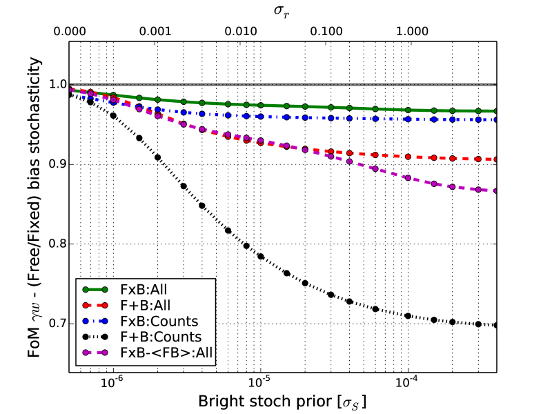
Fig. 12 shows ratios between free and fixed bias stochasticity, when marginalizing over the uncertainty only for the Bright population. On the x-axis is an absolute prior added to each Bright bias stochasticity parameter. The ratio can be understood as the fraction of the FoMs recovered from adding priors. For strong priors, on the left side of the graph, the priors effectively fix galaxy bias and the ratio naturally approaches unity. There is a clear difference between overlapping and non-overlapping surveys. Without priors, the F+B:Counts reduces to 70% of the value with known stochasticity. The difference is 96% of the original value when considering FxB:Counts. Also including lensing (:All), the overlapping surveys are less affected by the bias stochasticity uncertainties. Similar trends are found also for $\text{FoM}_{\gamma}$ (not shown), but with a much smaller change.

This figure (12) shows that overlapping samples are less affected by a galaxy stochasticity uncertainty. This contradicts Kirk et al. (2013), which found that marginalizing over bias stochasticity parameters significantly reduce the same-sky benefit (from a factor of 3.9 to 1.2). Previously in EG14a, we discussed their higher absolute gain from overlapping surveys. The main difference is Kirk et al. (2013) ignore the count-shear cross-correlation with photometric (Faint) lenses. This artificially increase the same-sky benefit, since the counts-shear signal with different galaxy lens populations are highly correlated (see subsection 2.5). Only using the counts-shear of one galaxy population would also increase their sensitivity the galaxy bias stochasticity.

4 Conclusion

This paper accompanies the previous forecast (paper-II, EG14a). These combined a photometric (Faint) and a spectroscopic (Bright) stage-IV survey to constrain the growth and expansion history by using a combination of weak lensing and galaxy clustering. In particular, these papers focused on the gain from observing the same area with both surveys. For the combined constraints, knowing the galaxy bias would increase the figure of merit ($\text{FoM}_{w\gamma}$) equivalent to 3-5 times larger area. Details of the galaxy bias affected both the same-sky benefit (i.e. FxB/F+B) and how much various effects contribute to the constraints. This paper (paper-III) studied how the bias impacts different aspects of the combined forecast.

Section 2 focused on the bias error and subsection 2.1 summarized the forecast assumptions. Then subsection 2.2 introduced the bias derivative formula, which includes the photo-z effect through the transition matrices (see Gaztañaga et al. (2012)) and also accounts for RSD and magnification. The next subsection (2.3) showed the fiducial bias error and how lensing contribute to the bias constraints. Subsection 2.4 stressed how ignoring the covariance between the cosmology and bias would lead to underestimate the value of overlapping surveys for constraining the bias.

Overlapping surveys both allow for additional cross-correlations and sample variance cancellations directly from overlapping volumes (see paper-II and EG14a). In subsection 2.5 we studied which counts-shear contribute to measuring the bias. From a covariance between the signals, the bias error only increase weakly when removing either lens population, but strongly when removing both. Subsection 2.6 studied the direct effect of overlapping volumes. The sample variance contribute most to the Bright sample, while the Faint sample benefit most from the additional cross-correlations.

Section 3 studied the effect of adding priors, bias parameterization and modelling of the bias stochasticity. Subsection 3.1 added uncorrelated priors in each bins on either the Bright or Faint bias. When adding bias priors, they directly affect the galaxy population and also the other galaxy population through the cross-correlations. Completely fixing the galaxy bias reduce the same-sky benefit (see paper-II). If adding priors to either population, the $\text{FoM}_{w\gamma}$ (FxB/F+B):All same-sky ratio only change weakly. For $\text{FoM}_{\gamma}$ the Bright sample would completely dominate $\text{FoM}_{\gamma}$ if fixing the Bright bias. Subsection 3.2 tested the sensitivity to the bias parameterization, which fiducially use one-bias-per-bin. Including more Bright redshift bins reduced the sensitivity to the bias. We further compared to a bias interpolated between $n$ redshift pivot points. For $n=3$ the $\text{FoM}_{w\gamma}$ results agreed within 10% and the one-bias-per-bin is therefore a reasonable bias parameterization.

Appendix A studied how the fiducial bias change the forecast. Changing the bias amplitude affects both the combined constraints and the relative performance of various probes (clustering, RSD, WL). In subsection 2.7 the dark energy ($\text{FoM}_{\text{DETF}}$) and growth ($\text{FoM}_{\gamma}$) constrains respectively increase and decrease when increasing the Bright galaxy bias amplitude. Increasing the Bright/spectroscopic bias reduces the shot-noise and therefore improving the dark energy constraints. The growth constraints reduced since the relative contribution of RSD, which is important to measure $\gamma$, decrease for a higher bias. In subsection A.1 and A.2 we studied respectively respectively the relative contribution of RSD and BAO. Last, subsection 14 investigated how the Faint bias amplitude impacts shear and magnification. A higher Faint bias increased the importance of WL for dark energy constraints ($\text{FoM}_{w}$) and reduces the impact of magnification. Appendix B showed how bias errors depend on photo-z and density.

The fiducial bias is deterministic. Subsection 3.3 introduced a simple stochastic galaxy bias model and related the definition to the commonly used correlation coefficient $r$ (see also Dekel & Lahav (1999)). Increasing the Bright bias stochasticity reduced the same-sky benefit (FxB:All/F+B:All), with the sample variance cancellation being more affected than the Bright-Faint cross-correlations. If marginalizing over an uncertainty in the bias stochasticity (see subsection 3.4), the overlapping photometric and spectroscopic (FxB) are less affected (than F+B). Thus overlapping surveys not only provide a better figure of merit (equivalent to 50% larger area) than separate surveys, but they are more robust to systematic errors, such as bias stochasticity or uncertainties in the bias evolution.

Appendix A Bias amplitude

Subsection 2.7 studied the absolute effect of shifting the bias amplitude. This appendix focus on the relative effect of RSD (subsection A.1), BAO (subsection A.2) and WL (subsection A.3).

A.1 Redshift Space Distortions

Figure 13: The effect of RSD when scaling the Bright bias amplitude. On the x-axis is the Bright bias amplitude relative to the fiducial value. The figure shows the $\text{FoM}_{w\gamma}$ redshift/real space ratio. A ratio above unity means RSD increase the FoM. The lines corresponds to FxB:All, F+B:All, FxB:Counts, FxB-$\left<\text{FB}\right>$:Counts and F+B:Counts.

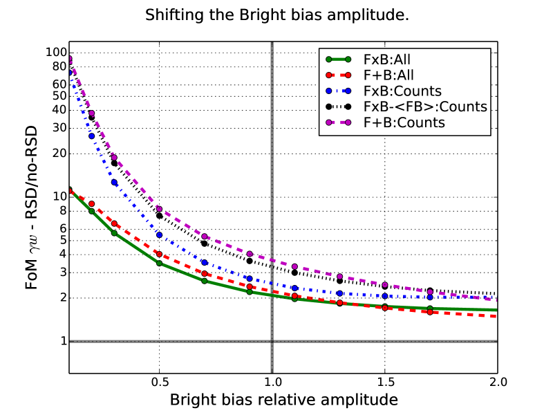
Fig. 13 shows the $\text{FoM}_{w\gamma}$ redshift/real space forecast ratios, varying the Bright bias amplitude. As in the previous subsections, we do not show the ratio when varying the Faint bias. The benefit of RSD decrease for a higher Bright bias, which confirms the importance of RSD in Fig. 7. As expected, the largest contribution comes when only including Counts. For low Bright biases the RSD is the main contribution to the signal. The ratios looks dramatically high (60-100) when only including galaxy counts. While the effect of RSD is more important for a low bias, the RSD increasing the auto-correlation amplitude and therefore lower the impact of shot-noise. Without the Bright galaxy shot-noise (not shown), the RSD/no-RSD at low Bright bias drops. For a relative bias of 0.1, the ratio is 10(17) for FxB:Counts(F+B:Counts).

For $\text{FoM}_{w\gamma}$ the RSD/no-RSD ratio is above unity and RSD improve the constraints. This conclusion depends on the FoM and the galaxy density. The RSD contribute strongly to measuring $\gamma$, but less for the dark energy constraints. For $\text{FoM}_{\text{DETF}}$ and sufficient density, the RSD signal decrease the constraint (not shown). While the additional RSD signal is good to measure $\gamma$, the RSD suppress cross-correlations between close redshift bins redshift (see paper-I). As seen in paper-II, the radial information in these cross-correlations contribute strongly to the dark energy constraints. This suppression therefore lower the constraints when including RSD.

At large Bright bias amplitudes the RSD/no-RSD ratio changes differently for overlapping (FxB) and non-overlapping (F+B) surveys. The similarity at low bias is due to a low density and disappear when removing the shot-noise (not shown). Because FxB include the Bright-Faint cross-correlations, one expect a smaller dependence on the RSD contribution in the Bright sample and smaller reduction in the RSD/no-RSD ratio. Notice also how FxB-$\left<\text{FB}\right>$:Counts is only slightly below FxB:Counts. While this trend is not the strongest, RSD is important for sample variance cancellations. Otherwise, the galaxy clustering of both populations is directly proportional to the matter overdensities. That would remove the benefit of using two tracers. This effects also contribute to the FxB ratios flattening for a high Bright bias.

A.2 Baryon Acoustic Oscillations (BAO)

Figure 14: The effect of BAO for different bias amplitudes. The $\text{FoM}_{w\gamma}$ ratios are between including or not BAO wiggles in the Eisenstein-Hu power spectrum. On the x-axis is a multiplicative bias amplitude relative to the fiducial Bright(Faint) bias. The lines corresponds to FxB:All, F+B:All, FxB:Counts, FxB-$\left<\text{FB}\right>$:Counts and F+B:Counts.

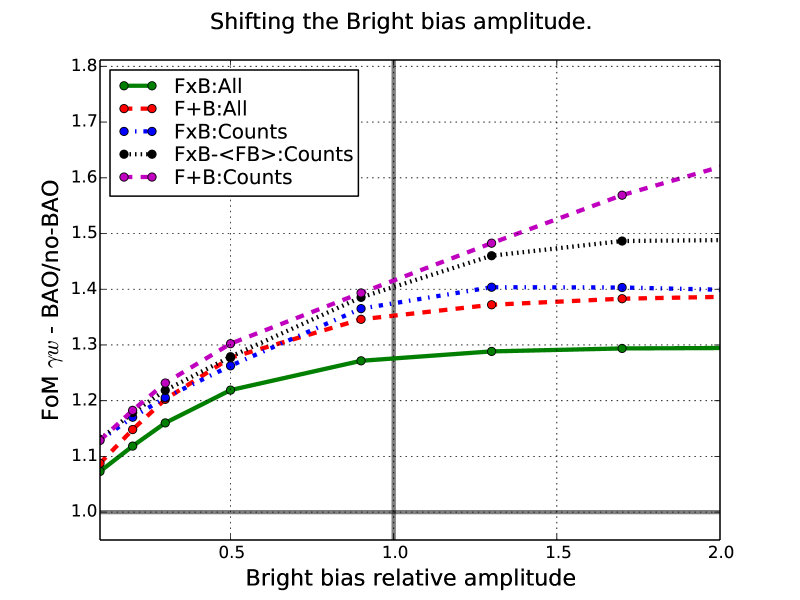
The BAO scale of 150 Mpc is a characteristic scale with a higher probability of finding a galaxy pair. In the 2D and 3D configuration space correlation function, the BAO is a significant peak, where the position is largely independent of the galaxy bias Eisenstein et al. (2005). Instead of only constraining cosmology from the peak position, these papers include the BAO signal through the 2pt correlation function. The advantage is utilizing the full power spectrum, but it does require modelling the galaxy bias. To estimate the importance of BAO, the Eisenstein-Hu (EH) model can predict the dark matter power spectrum with and without BAO wiggles. We check how BAO impacts the constraints by calculating the FoMs with and without the BAO wiggles.

Fig. 14 shows the BAO/no-BAO $\text{FoM}_{w\gamma}$ forecast ratios when varying the Bright bias amplitude. The BAO peak is effective in measuring the expansion, but not the growth. Including BAO improve $\text{FoM}_{w\gamma}$($\text{FoM}_{\text{DETF}}$) with 30% (23%), while $\text{FoM}_{\gamma}$ decrease with 1%. Since BAO has largest effect on the dark energy constraints, trends in this figure can be compared to $\text{FoM}_{\text{DETF}}$. Similar to the absolute $\text{FoM}_{\text{DETF}}$ constraints, the BAO/no-BAO ratio trend change with the Bright galaxy density. Without shot-noise, the BAO/no-BAO ratios above a relative bias amplitude of 0.5 is close to flat (not shown). A higher bias is therefore advantageous for reducing the shot-noise, which is why Red Luminous Galaxies (LRGs) are often targeted for BAO studies (Eisenstein et al., 2005; Gaztañaga, Cabré & Hui, 2009).

A.3 Galaxy shear and Magnification.

Weak lensing also depend on the galaxy bias. For the signal, the counts-shear cross-correlations and magnification are nearly proportional to the foreground bias amplitude. Magnification, which change the observed number counts through lensing (see paper-I), is included by default. While the measurement noise is independent of bias, the dominant (cosmic variance) contribution also scale linear with bias. In this subsection, we first study the effect of both weak lensing signals when shifting the Faint bias amplitude. Next we focus on the contribution from magnification.

Figure 15: The effect of the Faint bias amplitudes on the weak lensing contribution. On the x-axis is a multiplicative amplitude relative to the fiducial Faint bias. Ratios in the top panel show the WL/no-WL ratios, where WL is the fiducial forecast and no-WL remove all WL signals (counts-shear, shear-shear and magnification). In the bottom panel the no-Magnification forecast set the magnification slopes (see paper-I) to zero.

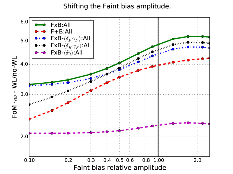
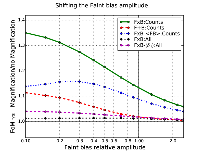
Fig. 15 (top panel) shows the WL/no-WL $\text{FoM}_{w\gamma}$ ratio. In FxB:All the signal include the shear-shear and counts-shear cross-correlations with both populations as lenses. This configuration naturally has the largest effect of weak lensing. The next two lines are FxB-$\left<\delta_{B}\gamma_{F}\right>$(FxB-$\left<\delta_{F}\gamma_{F}\right>$), which is FxB:All, but removing the counts-shear correlations with Bright(Faint) lenses. In paper-II the Faint lenses contributed slightly stronger to the forecast (see also subsection 2.5). The relative strength of different lens populations depend on the bias amplitudes, which results in the lines crossing. For non-overlapping surveys (F+B:All), one can only measure counts-shear with Faint lenses and result in F+B:All and FxB-$\left<\delta_{B}\gamma_{F}\right>$ following a similar trend. Finally, the line FxB-$\left<\delta\>\gamma\right>$ is including no counts-shear correlations and the trend is therefore flat.

The bottom panel Fig. (15) shows the magnification /no-magnification $\text{FoM}_{w\gamma}$ ratio. Magnification affect number counts in two ways. Foreground foreground matter over and under densities respectively magnify and de-magnified background galaxy fluxes and areas. The magnified fluxes can enter/leave a magnified limited sample, changing the total number of galaxies, while the magnified area modify the galaxy density. Here the magnification slope (magnification strength) equals the fiducial configuration in paper-II (see paper-II, Fig. 1).

The effect of number counts magnification is small compared to WL, RSD or BAO. For FxB:All (flattest ratio) magnification only increase $\text{FoM}_{w\gamma}$ with $\sim 1\%$, while the effect is 15% for FxB:Counts. This discussion therefore focus on the number counts results (Counts). In FxB-$\left<\text{FB}\right>$ the surveys overlap, which give sample variance cancellations, but does not include the Bright-Faint cross-correlations. This reduce the bias constraints and therefore the magnification constrains. The non-overlapping surveys (F+B) does not have sample variance cancellations from overlapping volumes and the ratio drops further. Finally, could the low magnification effect be caused by the counts-shear and magnification signal being proportional? The line FxB-$\left<\delta\>\gamma\right>$ is FxB:All, but removing all counts-shear cross-correlations or equivalently FxB:Counts adding shear-shear. The effect of magnification is also low when including the shear-shear lensing observable.

A lower Faint bias amplitude improve the forecast. One can understand this from the signal-to-noise. The variance of the magnification signal when assuming Gaussian fluctuations (see paper-II) is

$$\Delta^{2}C_{\delta_{i}\delta_{j}} =N^{-1}(l)[C_{\delta_{i}\delta_{i}}C_{\delta_{j}\delta_{j}}+C^{2}_{\delta_{i}\delta_{j}}]$$ (17)

$$\approx N^{-1}(l)C_{\delta_{i}\delta_{i}}C_{\delta_{j}\delta_{j}}$$ (18)

where $i$ and $j$ are the two redshift bins. For well separated bins in photo-z space, the auto-correlation terms dominate, which least to the approximation in the second line. If ignoring RSD, magnification-magnification correlations and the shot-noise, the magnification signal-to-noise is

$$S/N\approx\left|\frac{\alpha_{j}}{b_{j}}\right|\sqrt{N(l)}\frac{C_{m_{i}\gamma_{j}}}{\sqrt{C_{m_{i}m_{i}}C_{m_{j}m_{j}}}}$$ (19)

where $\alpha_{j}$ and $b_{j}$ are respectively the magnification slope and the galaxy bias in bin $j$. The $C_{m_{i}m_{i}}$ and $C_{m_{j}m_{j}}$ terms are respectively the matter auto-correlations in bin $i$ and $j$. This approximation is invalid for low Faint bias amplitudes. Eq. 19 shows two important criteria for magnification. Higher magnification slope increase the signal, while a lower bias of the background population decrease the errors. This criteria can be useful if focusing solely on magnification. To optimize the combined constraints, one should however focus on RSD, BAO and WL, since they contribute stronger.

Appendix B Photometric redshifts and galaxy densities

B.1 Photometric redshifts

Figure 16: The impact of the Bright photo-z on the bias error. Lines show the spec-z/photo-z bias error ratios. On the x-axis is the Gaussian photo-z (units of (1+z)) of the Bright sample. The top(bottom) panel show the ratios for the Bright(Faint) bias.

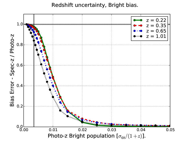
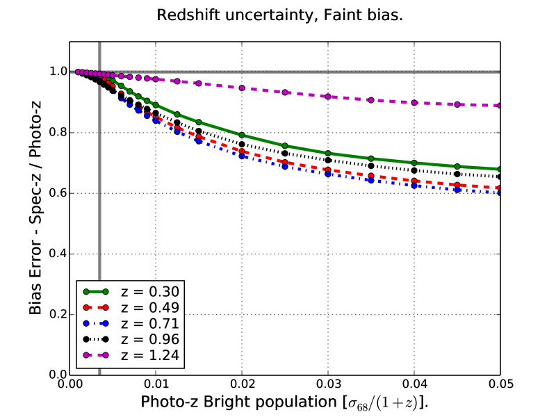
The bias measurements are affected by redshift uncertainties. Our two fiducial galaxy samples are: a photometric (Faint) and spectroscopic (Bright) with respectively $0.05(1+z)$ and $0.001(1+z)$ Gaussian redshift uncertainties. Since the Faint photo-z is broad, the Faint sample is analyzed in broad redshift bins. Improving the Faint photo-z would only substantially change the forecast if also using narrow bins for the Faint sample. We focus instead on the Bright redshift uncertainty and fix the Faint photo-z to the fiducial value.

Fig. 16 shows the FxB:All Bright bias error ratio between the case of using spectroscopic (Bright) sample and the case of including redshift uncertainties (photo-z) in the Bright sample. A vertical line (0.0035) show the expected photo-z precision for the PAU narrow band survey (Martí et al., 2014). The PAU photo-z would for the Bright population recover 90% of the bias error, with the Faint bias being nearly unaffected. However, note that this conclusion depends strongly on the Bright population redshift bin width, which fiducially is $\Delta z=0.01(1+z)$ (see paper-I, section 3.3). Reducing the Bright redshift accuracy from spec-z to a photo-z of $0.01(1+z)$ doubles the error on the Bright bias, which illustrate how better photo-z than the typical bin width is important when constraining cosmology with galaxy clustering.

The Bright bias ratios (Fig.16, top panel) approaches zero for a typical photometric redshift. Analyzing the bright sample with 72 narrow redshift bins and one bias parameter per bin is clearly not possible without accurate redshifts. The Faint galaxy bias (bottom panel) is affected through the Bright-Faint cross-correlations, sample variance cancellation and the uncertainty in cosmological parameters. These effects are less direct and the Faint bias error declines slower with increasing Bright photo-z, reaching asymptotic values of $\sim$0.6-0.7 and larger for high redshifts. When increasing the Bright photo-z, the Faint bias can still be measured through the Faint clustering and counts-shear cross-correlations.

Figure 17: The same-sky bias error benefit when varying the Bright photo-z. Lines are the Faint bias error ratios between non-overlapping and overlapping surveys. On the x-axis is the Bright sample Gaussian photo-z (units of (1+z)). The forecast include galaxy counts and shear (FxB:All).

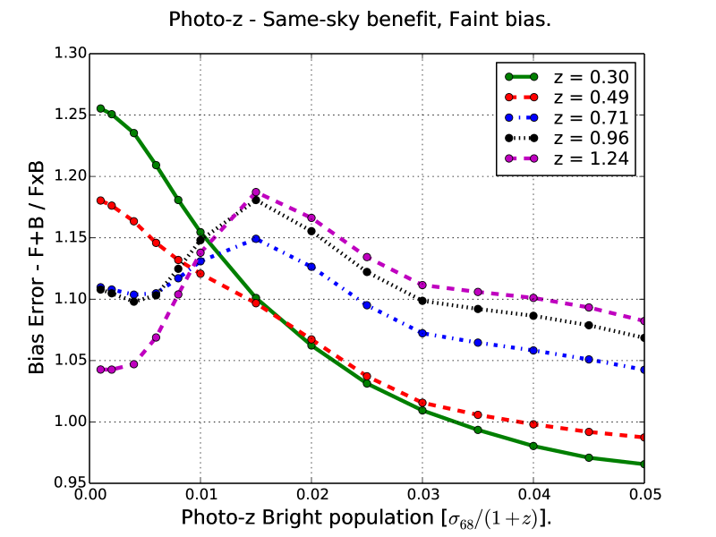
Fig. 17 shows the same-sky ratio, which is the bias error ratio between non-overlapping and overlapping galaxy surveys. Values below unity means overlapping surveys improve the bias measurement. For both FxB and F+B, a higher photo-z result in higher bias errors and the absolute errors increase strongly for all configurations (All, Counts). An increasing or decreasing ratio results from errors growing faster for either overlapping or non-overlapping surveys. For $\sigma_{z}\lesssim 0.01(1+z)$ the Bright sample alone becomes less able to constrain the bias, increasing the value of overlapping samples. When the photo-z increase and the nearby bins becomes more correlated, which reduce the same-sky benefit ratios. With only galaxy counts, the same-sky ratio change less (not shown).

B.2 Galaxy density

Figure 18: Impact of the galaxy density on the bias error. Each line show the FxB:All bias error, normalized to the errors for the fiducial Bright density (0.4 gal/sq.arcmin) for different redshift bins (see legend). The top(bottom) panel show the Bright(Faint) bias error ratio.

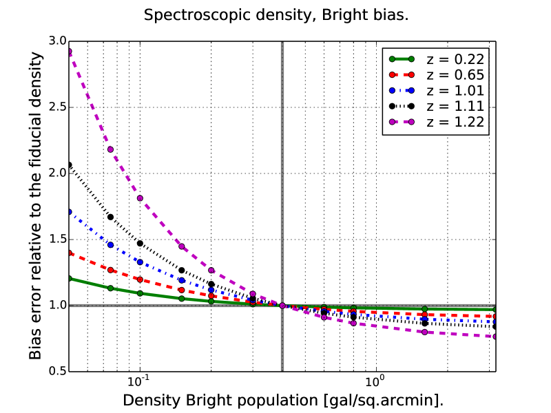
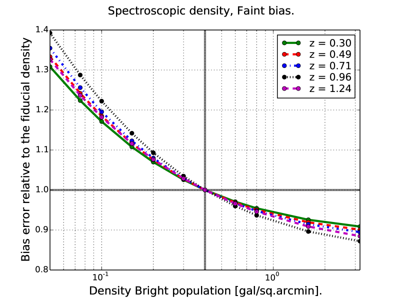
The galaxy density also change the cosmology and galaxy bias forecasts. This subsection study the effect of the spectroscopic density directly on the bias error. The fiducial photometric (Faint) sample is dense and varying its density only introduce small changes in the bias error, although it impacts cosmological constraint through e.g. the shear-shear measurement. For the related FoM forecast, see EG14a.

In Fig.18 we show the bias error when varying the Bright galaxy density and normalizing the error to unity for the fiducial density of the Bright sample (0.4 gal/sq.arcmin). As expected, the bias error decrease monotonically with higher galaxy density. The galaxy sample is less dense at high redshifts, which leads to the error on bias improving most for the highest redshift bins. When the Bright galaxy population is 0.1 gal/$\text{arcmin}^{2}$, which is $25\%$ of the fiducial value, the Bright bias error is 20-80$\%$ higher than the fiducial error. The Faint bias (bottom panel) benefits indirect through Bright-Faint cross-correlations and sample variance cancellation, therefore it depends weaker on the Bright galaxy density. Decreasing the Bright density to 0.1 gal/$\text{arcmin}^{2}$ results in 20% increase in the redshift error for most redshift bins. When increasing the density beyond the fiducial value, both populations show small improvements. This is compatible with the FoM saturation around 0.4 gal/sq.arcmin in EG14a.

References

- Albrecht et al. (2006) Albrecht A. et al., 2006, ArXiv e-prints, 0609591
- Anderson et al. (2014) Anderson L. et al., 2014, MNRAS, 439, 83
- Anderson et al. (2012) Anderson L. et al., 2012, MNRAS, 427, 3435
- Asorey, Crocce & Gaztañaga (2014) Asorey J., Crocce M., Gaztañaga E., 2014, MNRAS, 445, 2825
- Asorey et al. (2012) Asorey J., Crocce M., Gaztañaga E., Lewis A., 2012, MNRAS, 427, 1891
- Bardeen et al. (1986) Bardeen J. M., Bond J. R., Kaiser N., Szalay A. S., 1986, ApJ, 304, 15
- Bel, Hoffmann & Gaztañaga (2015) Bel J., Hoffmann K., Gaztañaga E., 2015, ArXiv e-prints
- Bernstein & Cai (2011) Bernstein G. M., Cai Y.-C., 2011, MNRAS, 416, 3009
- Blanton et al. (2000) Blanton M., Cen R., Ostriker J. P., Strauss M. A., Tegmark M., 2000, ApJ, 531, 1
- Cacciato et al. (2013) Cacciato M., van den Bosch F. C., More S., Mo H., Yang X., 2013, MNRAS, 430, 767
- Cai & Bernstein (2012) Cai Y.-C., Bernstein G., 2012, MNRAS, 422, 1045
- Clerkin et al. (2015) Clerkin L., Kirk D., Lahav O., Abdalla F. B., Gaztañaga E., 2015, MNRAS, 448, 1389
- Contreras et al. (2013) Contreras C. et al., 2013, MNRAS, 430, 924
- Coupon et al. (2012) Coupon J. et al., 2012, A&A, 542, A5
- de Jong et al. (2013) de Jong J. T. A., Verdoes Kleijn G. A., Kuijken K. H., Valentijn E. A., 2013, Experimental Astronomy, 35, 25
- de la Torre et al. (2013) de la Torre S. et al., 2013, A&A, 557, A54
- de Putter, Doré & Takada (2013) de Putter R., Doré O., Takada M., 2013, preprint (arXiv:1308.6070)
- Dekel & Lahav (1999) Dekel A., Lahav O., 1999, ApJ, 520, 24
- Di Dio et al. (2013) Di Dio E., Montanari F., Durrer R., Lesgourgues J., 2013, ArXiv e-prints
- Eisenstein et al. (2007) Eisenstein D. J., Seo H.-J., Sirko E., Spergel D. N., 2007, ApJ, 664, 675
- Eisenstein, Seo & White (2007) Eisenstein D. J., Seo H.-J., White M., 2007, ApJ, 664, 660
- Eisenstein et al. (2005) Eisenstein D. J. et al., 2005, ApJ, 633, 560
- Eriksen & Gaztanaga (2014a) Eriksen M., Gaztanaga E., 2014a, (arXiv:1412.8429) (EG14a)
- Eriksen & Gaztanaga (2014b) Eriksen M., Gaztanaga E., 2014b, (arXiv:1412.2208) (paper-I)
- Eriksen & Gaztanaga (2015) Eriksen M., Gaztanaga E., 2015, (arXiv:1502.03972) (paper-II)
- Font-Ribera et al. (2014) Font-Ribera A., McDonald P., Mostek N., Reid B. A., Seo H.-J., Slosar A., 2014, J. Cosmology Astropart. Phys, 5, 23
- Frieman & Gaztanaga (1994) Frieman J. A., Gaztanaga E., 1994, ApJ, 425, 392
- Fry (1996) Fry J. N., 1996, ApJ, 461, L65
- Gaztañaga, Cabré & Hui (2009) Gaztañaga E., Cabré A., Hui L., 2009, MNRAS, 399, 1663
- Gaztañaga et al. (2012) Gaztañaga E., Eriksen M., Crocce M., Castander F. J., Fosalba P., Marti P., Miquel R., Cabré A., 2012, MNRAS, 422, 2904
- Gaztañaga et al. (2005) Gaztañaga E., Norberg P., Baugh C. M., Croton D. J., 2005, MNRAS, 364, 620
- Gaztañaga & Scoccimarro (2005) Gaztañaga E., Scoccimarro R., 2005, MNRAS, 361, 824
- Heymans et al. (2013) Heymans C. et al., 2013, MNRAS, 432, 2433
- Ivezic et al. (2008) Ivezic Z. et al., 2008, ArXiv e-prints
- Kaiser (1984) Kaiser N., 1984, ApJ, 284, L9
- Kirk et al. (2013) Kirk D., Lahav O., Bridle S., Jouvel S., Abdalla F. B., Frieman J. A., 2013, preprint (arXiv:1307.8062)
- Laureijs et al. (2011) Laureijs R. et al., 2011, preprint (arXiv:1110.3193)
- Le Fèvre et al. (2013) Le Fèvre O. et al., 2013, A&A, 559, A14
- Levi et al. (2013) Levi M. et al., 2013, preprint (ArXiv:1308.0847)
- Martí et al. (2014) Martí P., Miquel R., Castander F. J., Gaztañaga E., Eriksen M., Sánchez C., 2014, MNRAS, 442, 92
- McDonald & Seljak (2009) McDonald P., Seljak U., 2009, J. Cosmology Astropart. Phys, 10, 7
- Nock, Percival & Ross (2010) Nock K., Percival W. J., Ross A. J., 2010, MNRAS, 407, 520
- Nusser & Davis (1994) Nusser A., Davis M., 1994, ApJ, 421, L1
- Perlmutter et al. (1999) Perlmutter S. et al., 1999, ApJ, 517, 565
- Planck Collaboration et al. (2015) Planck Collaboration et al., 2015, preprint (ArXiv:1502.01589)
- Press & Schechter (1974) Press W. H., Schechter P., 1974, ApJ, 187, 425
- Riess et al. (1998) Riess A. G. et al., 1998, AJ, 116, 1009
- Scoccimarro et al. (2001) Scoccimarro R., Sheth R. K., Hui L., Jain B., 2001, ApJ, 546, 20
- Sefusatti et al. (2006) Sefusatti E., Crocce M., Pueblas S., Scoccimarro R., 2006, Phys. Rev. D, 74, 023522
- Seljak & Warren (2004) Seljak U., Warren M. S., 2004, MNRAS, 355, 129
- Shoji, Jeong & Komatsu (2009) Shoji M., Jeong D., Komatsu E., 2009, ApJ, 693, 1404
- Simpson et al. (2013) Simpson F. et al., 2013, MNRAS, 429, 2249
- Tegmark & Peebles (1998) Tegmark M., Peebles P. J. E., 1998, ApJ, 500, L79
- The Dark Energy Survey Collaboration (2005) The Dark Energy Survey Collaboration, 2005, preprint (arXiv:astro-ph/0510346)
- Weinberg et al. (2013) Weinberg D. H., Mortonson M. J., Eisenstein D. J., Hirata C., Riess A. G., Rozo E., 2013, Phys. Rep., 530, 87
- Zheng et al. (2005) Zheng Z. et al., 2005, ApJ, 633, 791