NuSTAR Observations of the Young, Energetic Radio Pulsar PSR B1509$-$58

Abstract

We report on Nuclear Spectroscopic Telescope Array (NuSTAR) hard X-ray observations of the young rotation-powered radio pulsar PSR B1509$-$59 in the supernova remnant MSH 15$-$52. We confirm the previously reported curvature in the hard X-ray spectrum, showing that a log parabolic model provides a statistically superior fit to the spectrum compared with the standard power law. The log parabolic model describes the NuSTAR data, as well as previously published $\gamma$-ray data obtained with COMPTEL and AGILE, all together spanning 3 keV through 500 MeV. Our spectral modelling allows us to constrain the peak of the broadband high energy spectrum to be at 2.6$\pm$0.8 MeV, an improvement of nearly an order of magnitude in precision over previous measurements. In addition, we calculate NuSTAR spectra in 26 pulse phase bins and confirm previously reported variations of photon indices with phase. Finally, we measure the pulsed fraction of PSR B1509$-$58 in the hard X-ray energy band for the first time. Using the energy resolved pulsed fraction results, we estimate that the pulsar’s off-pulse emission has a photon index value between 1.26 and 1.96. Our results support a model in which the pulsar’s lack of GeV emission is due to viewing geometry, with the X-rays originating from synchrotron emission from secondary pairs in the magnetosphere.

1. Introduction

PSR B1509$-$58 is a young, energetic rotation-powered pulsar discovered in the soft X-ray band using the Einstein Observatory (Seward & Harnden 1982) and soon afterwards detected in the radio band (Manchester et al. 1982). It has period $\sim$150 ms, period derivative $\sim$1.5 $\times 10^{-12}\rm s\ s^{-1}$ and a high spin-down luminosity of $\dot{E}=1.7\times 10^{37}\rm erg~{}s^{-1}$. Assuming the standard magnetic dipole model, its characteristic spin-down age is $\sim$1600 years and inferred surface magnetic field at the equator is $\sim 1.5\times 10^{13}$ G, higher than the lowest estimation of $B_{\rm dip}\simeq 6\times 10^{12}\rm G$ for a magnetar (Rea et al. 2013). The pulsar lies in the centre of the supernova remnant MSH 15$-$52, which has a complex structure with thermal and non-thermal emission, which is largely powered by the pulsar (Tamura et al. 1996). Recently, NuSTAR observations of the MSH 15$-$52 and its pulsar wind nebula (PWN) region by An et al. (2014) revealed clear evidence for synchrotron burnoff in the PWN, spectral softening with distance from the pulsar, and an interesting shell-like structure in the $N_{\rm H}$ map.

The aforementioned NuSTAR observations also offer a new window into the hard X-ray emission of the central pulsar itself, the subject of this work. PSR B1509$-$58 is one of the brightest rotation-powered X-ray pulsars in the sky and has been observed by many X-ray and soft $\gamma$-ray telescopes, for example, Ginga (Kawai et al. 1993), OSSE (Matz et al. 1994), WELCOME (Gunji et al. 1994), RXTE (Marsden et al. 1997), COMPTEL (Kuiper et al. 1999), AGILE (Pilia et al. 2010), BeppoSAX (Cusumano et al. 2001), and Fermi LAT (den Hartog et al. in preparation). Thanks to NuSTAR’s wide energy range in the hard X-ray band and unique hard X-ray focusing ability therein, NuSTAR observations of PSR B1509$-$58 can shed new light on the pulsar’s hard X-ray spectrum.

The pulsar’s spectrum in the hard X-ray band has long been of interest, in part because the source’s large flux enables detailed studies not possible in most rotation-powered pulsars. Based on BeppoSAX and COMPTEL observations, Cusumano et al. (2001) reported that the spectral energy distribution of PSR B1509$-$58 is well represented by a logarithmic parabolic function characterized by a linear dependence of the spectral slope upon the logarithm of energy from $\sim$1 keV to $\sim$30 MeV, rather than the simple power-law model so ubiquitously assumed for rotation-powered pulsar spectra. The spectral bending in PSR B1509$-$58 was reported to be detectable also in the keV energy range. If correct, this has important implications for the high energy emission mechanism. However, BeppoSAX was an X-ray astronomy satellite that consisted of three instruments operating in different energy bands (Boella et al. 1997), and slight systematic cross-calibration discrepancies among these three instruments have been reported by Kirsch et al. (2005). Hence confirmation of the claim of spectral curvature from BeppoSAX data is important to obtain, particularly with a mission like NuSTAR which covers the full 3–79 keV band with a single instrument. This, when combined with recent soft $\gamma$-ray observations, can in principle provide vastly improved constraints on the full high-energy spectrum, which could help better determine the peak spectral energy and ultimately address the curious low-energy cutoff seen in the high-energy $\gamma$-ray spectrum from this source (Abdo et al. 2010).

In this paper, we present timing and spectral analyses of PSR B1509$-$58 data obtained by NuSTAR as well as the Chandra X-ray Observatory. In Section 2, we describe our observations and data reduction. In Section 3, we present our analysis and results. In Section 4 we discuss the results and in Section 5 provide a summary.

2. Observations

NuSTAR is the first focusing X-ray telescope that operates above 10 keV (Harrison et al. 2013). It consists of two co-aligned hard X-ray grazing incidence telescopes, which focus onto two independent solid-state focal plan modules, and produce two spectra in each observation. The angular resolution of the observatory is 18^′′ FWHM, with a half power diameter of 58^′′. Both telescopes operate in the energy band from 3 to 79 keV and each provides an energy resolution of 400 eV FWHM at 10 keV and 0.9 keV at 60 keV. The temporal resolution is 2 $\mu$s, and the timing accuracy is 1–2 ms.

Four NuSTAR observations were made of the region containing PSR B1509$-$58 as well as its PWN in June and August of 2013, with a total exposure time of 178.9 ks (see An et al. 2014). In every observation, the two telescopes each produced a spectrum for a total of eight spectra. We also analyzed an archival Chandra observation made with the High Resolution Camera (HRC) in June 2005, with an exposure time of 44.9 ks. The HRC is sensitive within 0.08–10 keV. Since the spectral response of HRC is extremely limited, we used the Chandra data only for the timing analysis below. Table 1 summarizes the observations.

Table 1Summary of Observations

Observatory	Obs. ID	Start Epoch	Start Date	Stop Date	Exposure
		(MJD)	(UT)	(UT)	(ks)
NuSTAR	40024004002	56450.9	2013Jun07	2013Jun08	43.4
NuSTAR	40024002001	56451.8	2013Jun08	2013Jun09	42.6
NuSTAR	40024003001	56452.6	2013Jun09	2013Jun10	44.3
NuSTAR	40024001002	56519.6	2013Aug15	2013Aug16	48.6
Chandra (HRC)	5515	53534.0	2005Jun13	2005Jun13	44.9

The NuSTAR data were processed with HEASOFT v6.15.1, nupipeline v1.3.1, and the Calibration Database (CALDB) files from 20131223. Standard Level 2 cleaned events files were generated for further analysis. The Chandra data were reprocessed with chandra_repro in CIAO 4.5 in order to use the most recent calibration files.

3. Data Analysis and Results

3.1. Timing Analysis

From each NuSTAR observation, pulsar events were extracted in the 3–79 keV energy band using a circular region of radius 30^′′ centered on the pulsar. We then applied a correction to convert photon arrival times to the equivalent time at the solar system barycenter (Barycentric Dynamical Time) using the DE200 ephemeris. We verified that the pulse periods at each epoch were consistent with those predicted by the ephemeris of Livingstone & Kaspi (2011).

To measure the properties of the X-ray pulsations of PSR B1509$-$58, the background must be carefully subtracted. The background consists of two components: detector background and PWN. For the NuSTAR observations, the detector background was extracted with an aperture of radius 45^′′ in a pulsar-free and PWN-free region on the same detector chip with the pulsar. We also tried different background regions and found that all results in our analysis were independent of the exact choice of region. The PWN, however, is important to consider because of NuSTAR’s broad point spread function (PSF), which will be described later in this section.

We produced pulse profiles using the NuSTAR data in 14 energy bandpasses from 3–79 keV (Fig. 1). Each pulse profile contained 64 bins and the number of events in each bin was at least 20. To obtain the pulsed component from a pulse profile, we determined the smallest photon count value among the 64 bins, used it as the off-pulse level, and subtracted this off-pulse value from each of the 64 bins.

In order to search for pulse profile evolution with energy, we compared the shapes of the pulse profiles in the 14 energy bands. We scaled them by dividing each with the total photon counts in that pulse profile. We chose the pulse profile of 3–79 keV as a reference, subtracted each of the 14 normalized profiles from it, and tested $\chi^{2}$. No significant variation in shape was detected, and the residuals appeared to be random. The $\chi^{2}$ test showed that the probability of the pulse profiles being the same in shape with the reference is above 40% for 11 energy bands. The most suspicious one had a probability of 0.24%, still not sufficiently small to indicate a disagreement in shape, considering the number of trials. Furthermore, shifts in phase could indicate that emission regions vary with energy. To check this, we performed a cross correlation of each pulse profile with the reference, but no significant phase shift was seen for any profile.

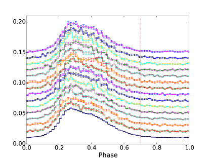
Figure 1.— Pulse profiles from NuSTAR observations in various energy bands: from bottom to top are energy band of 3–79 keV, 3–4 keV, 4–5 keV, 5–6 keV, 6–7 keV, 7–8 keV, 8–9 keV, 9–10 keV, 10–11 keV, 11–12 keV, 12–14 keV, 14–16 keV, 16–19 keV, 19–25 keV and 25–79 keV, respectively. Phase zero was selected approximately around the point where the pulsation starts. The histograms each contain 64 bins. Values of the y-axis don’t have physical meaning. No significant change in shape was found in different energy bandpasses. We used phase 0.7–1 (vertical dotted line) as the off-pulse component in Section 3.2.

The pulsed fraction can be defined in several ways. Here we chose the RMS pulsed fraction, as well as an intuitive definition based on the area under the pulse. The RMS pulsed fraction is defined as (Dib et al. 2009)

$$PF_{\rm RMS}=\frac{\sqrt{2\sum_{k=1}^{8}((a_{k}^{2}+b_{k}^{2})-(\sigma_{a_{k}}^{2}+\sigma_{b_{k}}^{2}))}}{a_{0}}.$$

Here, $a_{k}$=$\frac{1}{N}\sum_{i=1}^{N}r_{i}\cos(2\pi\phi_{i})$, $b_{k}$=$\frac{1}{N}\sum_{i=1}^{N}r_{i}\sin(2\pi\phi_{i})$, and $\sigma_{a_{k}}$, $\sigma_{b_{k}}$ are the uncertainties in $a_{k}$ and $b_{k}$ respectively. ${\phi_{i}}$ is the phase, $N$ is the total number of phase bins, and $k$ refers to the number of Fourier harmonics.

The area pulsed fraction is

$$PF_{\rm area}=\frac{\sum_{i=1}^{N}(r_{i}-r_{\rm min})}{\sum_{i=1}^{N}r_{i}}.$$

Here, ${r_{i}}$ is the count number in the $i$th phase bin, $N$ is the total number of phase bins, and $r_{min}$ is the minimal count number in all bins.

Figure 2 displays the RMS and area pulsed fractions measured for pulse profiles in the 14 energy bands. Both the RMS and area pulsed fractions increase with energy between 3 and $\sim$19 keV and then approach a plateau at 19–79 keV. The RMS of the highest energy band is about 3$\sigma$ larger than that of the lowest band.

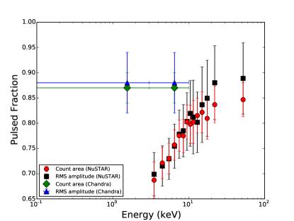
Figure 2.— RMS and area pulsed fractions in multiple energy bands from NuSTAR and Chandra observations. On the one hand, the NuSTAR results increase significantly between 3 to $\sim$19 keV and then approach a plateau within 19–79 keV: the RMS pulsed fraction of the highest energy band is about 3$\sigma$ larger than that of the lowest one. On the other hand, the Chandra results do not show any variation between 0.08–10 keV. Moreover, the RMS pulsed fraction of Chandra is consistent with NuSTAR’s results above 19 keV within 0.2$\sigma$.

To estimate the pulsed fraction that is free from PWN contamination (PWN-free), pulsed fractions were also measured from the Chandra HRC observation. The RMF of the Chandra HRC is complicated, so the energy-resolved HRC pulsed fractions (Fig. 2) should be regarded as as having been measured just in “soft” and “hard” bands, not the exact energy ranges. This does not change any result though, since we found the Chandra pulsed fraction value to be constant in these two bands. For the Chandra observation, we can ignore background contamination because of Chandra’s narrow PSF. Specifically, in the Chandra observation within 0.08–10 keV, there were 12100 events collected in the pulsar region ($R$=1.5^′′) while the number of background events collected within an annular region with $R_{in}$=2^′′ and $R_{out}$=4^′′ was 374. Hence the background contamination in the Chandra pulsar region would be 70/12100, which is ignorable, and the PWN-free pulsed fraction value could be measured directly.

We estimated the PWN contamination in 3–10 keV in the NuSTAR pulsar region using the Chandra HRC observation. In 0.08–10 keV, the Chandra observation had 8080 counts in an annular region with $R_{in}$=1.5^′′ and $R_{out}$=30^′′. We used PIMMS to convert this into the 3–10 keV NuSTAR counts assuming a power-law spectrum with a photon index of 1.7 (An et al. 2014), and the result was 12694 counts. In 3–10 keV, the NuSTAR data had 37927 counts in the pulsar region, so the PWN contamination is roughly 12694/37927, not ignorable. This implied a pulsed fraction of $\sim$66%, consistent within 3$\sigma$ with our NuSTAR measurements in 3–4 keV, 4–5 keV, 5–6 keV, 6–7 keV, 7–8 keV, 8–9 keV and 9–10 keV.

Figure 2 shows that the RMS and area pulsed fractions measured from Chandra HRC between 0.5–10 keV are higher than the results measured from NuSTAR in 3–10 keV, however, the Chandra results are consistent with the NuSTAR results above 19 keV to within 0.2$\sigma$. This suggests that the variation of pulsed fraction from NuSTAR is due to the variation in the PWN contribution, which decreases faster than the pulsar spectrum at higher energy. In Section 4, we will use these results to estimate contributions from the PWN and the pulsar’s off-pulse component, and discuss constraints on the photon index of the pulsar’s off-pulse component.

3.2. Phase-averaged and Pulsed Spectral Analysis

Table 2Cross Normalization Factors of Each Spectrum

Obs. ID	Cross Normalization Factor
40024004002A	1
40024004002B	$1.00\pm 0.014$
40024002001A	$0.789^{+0.014}_{-0.013}$
40024002001B	$0.794\pm 0.013$
40024003001A	$1.02\pm 0.015$
40024003001B	$1.04\pm 0.015$
40024001002A	$1.02\pm 0.016$
40024001002B	$1.03\pm 0.016$

Table 3Pulsed and Phase-averaged Spectral Analysis Results

Model	Photon Index	$\alpha$	$\beta$	$K$	Flux (3-79 keV)	$\chi^{2}/dof$	Null Probability
				[$10^{-3}\rm ph~{}cm^{-2}~{}s^{-1}keV^{-1}$]	[$10^{-10}\rm erg~{}cm^{-2}~{}s^{-1}$]
Power Law	$1.386\pm 0.007$	…	…	$3.70\pm 0.07$	$1.198\pm 0.014$	278/254	14.4%
Logpar	…	$1.16\pm 0.05$	$0.11\pm 0.02$	$2.81^{+0.16}_{-0.15}$	$1.136\pm 0.018$	254/253	$47.6\%$
Logpar	…	$0.96\pm 0.08$	$0.16\pm 0.04$	$1.8\pm 0.3$	$\sim 1.33$	…	…

Table 4Broadband Spectral Analysis Results at Different Energy Bands

Energy	$\alpha^{a}$	$\beta^{a}$	$K^{a}$	$\chi^{2}/dof$	Null Probability
			[$10^{-3}\rm ph~{}cm^{-2}~{}s^{-1}keV^{-1}$]
NuSTAR Results
3–79 keV	$1.09\pm 0.04$	$0.13\pm 0.02$	$2.47\pm 0.12$	295/260	$7\%$
3 keV–30 MeV	$1.104\pm 0.018$	$0.124\pm 0.007$	$2.51\pm 0.06$	298/263	$7\%$
3 keV–500 MeV	$1.083\pm 0.015$	$0.134\pm 0.005$	$2.45\pm 0.06$	301/265	$6\%$
Cusumano et al. (2001)
2-300 keV	$0.96\pm 0.08$	$0.16\pm 0.04$	$1.8\pm 0.3$	…	…
2 keV–30 MeV	$1.03\pm 0.05$	$0.13\pm 0.02$	$1.9\pm 0.1$	…	…

In order to examine the spectrum of the pulsed emission from the pulsar, we first defined phase interval 0–0.7 as the pulsed component and the mean count rate between phases 0.7–1.0 as the off-pulse component (see Fig.1). We extracted 3–79 keV pulsar events and produced pulsed spectra. The off-pulse level was then subtracted from the pulsed component to yield the pulsed spectrum. In every observation, the two telescopes each produced a spectrum, so we had eight spectra from these four NuSTAR observations (Section 2). Each of the eight spectra was grouped into at least 600 counts per energy bin and then fitted jointly to various models, using the software package XSPEC v12.8.1g and using $\chi^{2}$ minimization. To check the results, we also grouped the spectra into 20, 50, 100, 200 and 400 counts per bin. In each case, we used both the $\chi^{2}$ minimization, and the cstat statistic, which is for Poisson data. The results did not differ significantly, so we only report the results for the spectra that were grouped into 600 counts per bin, and fitted with $\chi^{2}$ minimization statistics.

We first fitted the pulsed spectra with an absorbed single power-law model over 3–79 keV. Since the NuSTAR data are not sensitive to a small change in the equivalent hydrogen column $N_{\rm H}$, we fixed it at the previously reported value $0.95\times 10^{22}\rm\ cm^{-2}$ (Gaensler et al. 2002). Cross normalization factors were introduced for each spectrum because each observation sampled the source in a different detector region, as shown in Table 2. Two of the normalization factors were below 1, since part of the pulsar field fell into the detectors’ chip gaps. We then tied all the fitting parameters except the cross normalization factors for each spectrum. Table 3 shows the result. Figure 3 shows the spectra and the fitted single power-law model. Since we used phase 0–0.7 to produce the pulsed spectra, the exposure time was 0.7 times smaller than it should be. We corrected the normalization parameter $K$ and flux results throughout the spectral analysis with a factor of $1/0.7$. With $\chi^{2}$ per degree of freedom (dof) 278/254, the null hypothesis that the power-law model describes our data had a probability of $p$ = 14.41%, so the result was acceptable. However, note in Figure 3 that a systematically curved trend is seen in the residuals. Curved trends are also visible in the residuals of the spectra grouped into at least 400 counts per bin, and of the rebinned plots of the spectra grouped into at least 200, 100, 50 and 20 counts per bin. These imply that the single power-law model may not be the optimal representation of our data.

Following the work of Cusumano et al. (2001), we next fitted the spectra with a logarithmic parabolic (logpar) model:

$$A(E)=K(E/E_{\rm p})^{-\alpha-\beta log(E/E_{\rm p}))}.$$ (1)

Here, $\alpha$ is the slope at the pivot energy ($E_{\rm p}$), $\beta$ is the curvature term, $K$ is the normalization factor and we fixed $E_{\rm p}$ at 1 keV, as Cusumano et al. (2001) did. The values obtained were $\alpha=1.16\pm 0.05$, $\beta=0.11\pm 0.01$ and $K=(2.81^{+0.16}_{-0.15})\times 10^{-3}$ ph cm^-2 s^-1 keV^-1. A positive $\beta$ value means that the spectrum becomes softer at higher energy. Table 3 and Figure 3 show the results and spectra. With $\chi^{2}$ per dof 254/253, the null hypothesis that the logpar model describes our data had a probability of $p$= 47.64%, and the model was acceptable.

To determine whether the improvement in $\chi^{2}$ using the logpar model is statistically valid, we performed the standard F-test to estimate the probability that the improvement in $\chi^{2}$ tests was by chance. We found the probability to be $1.5\times 10^{-6}$, so the logpar model is statistically a better description of the data than the power law. Also the residuals in Figure 3 do not show an obvious trend. To test the probability that the residuals were random, we performed the Runs test (also known as Wald–Wolfowitz test; Orlandini et al. 2012; Barlow 1989) in XSPEC. The result was 2% for the power-law model, so the curved trend seen in the residuals of Figure 3 is statistically significant. For the logpar model, the result was 8%, so statistically the residuals of Figure 3 are 4 times more likely to be randomly distributed than those of Figure 3. Hence, the logpar model provides a statistically superior fit to the spectrum compared with the standard power law.

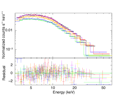
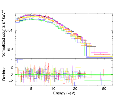
Figure 3.— (a) Top panel: NuSTAR observation data and the power-law model. Bottom panel: residual (data $-$ model). The power-law model is consistent with our data, $\chi^{2}$ per dof is 277.989/254 ($p$ = 14.41%). Note that a systematically curved trend is seen in the residuals. (b) Top panel: NuSTAR observation data and the logpar model. Bottom panel: residual (data $-$ model). The logpar model fits with our data better. $\chi^{2}$ per dof is 253.662/253 ($p$ = 47.64%). No visible trend is seen in the residuals. Eight Colors correspond to the eight spectra used in this analysis.

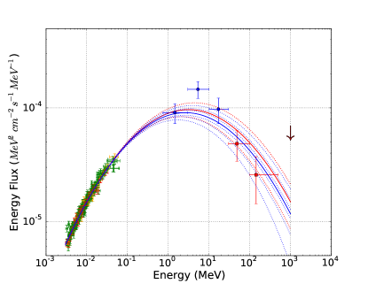
Figure 4.— The pulsed broadband energy spectrum of PSR B1509$-$58 from soft X-ray to $\gamma$-ray. The red squares are the AGILE observations in the 30–100 MeV and 100–500 MeV bands (Pilia et al. 2010). The arrow is the AGILE upper limit above 500 MeV band (Pilia et al. 2010). The blue circles are the COMPTEL observations in the 0.75–3 MeV, 3–10 MeV and 10–30 MeV bands (Kuiper et al. 1999). Data from 3-79 keV are from our NuSTAR observations. The solid red line is the logarithmic parabolic model obtained from NuSTAR data, and the dashed red lines show its $1\sigma$ range. The solid blue line is the logpar model obtained from all data from 3 keV to 500 MeV, and the dashed blue lines are its 1, 2 and 3$\sigma$ confidence regions.

3.3. Broadband Spectrum

We also produced a 3 keV– 500 MeV broadband spectrum for PSR B1509$-$58 and show it in Figure 4. The X-ray data are from NuSTAR and the $\gamma$-ray data are from observations made with COMPTEL (Kuiper et al. 1999) and AGILE (Pilia et al. 2010). Though significant pulsations were also detected by Fermi LAT (30– 1000 MeV) (den Hartog et al. in preparation), we did not use the results for our spectral analysis, because the Fermi SED of PSR B1509$-58$ was rather uncertain. Table 4 shows results obtained in 3–79 keV, 3 keV–30 MeV and 3 keV–500 MeV by fitting the logpar model (Equation 1) with data from NuSTAR, NuSTAR & COMPTEL, and NuSTAR & COMPTEL & AGILE, respectively. All fittings were acceptable. Note that we have unfolded the spectra in two slightly different methods and show the corresponding results in Tables 3 and 4, respectively. These two methods are compatible, since in the 3-79 keV band they produce results that are consistent within 2$\sigma$ (the second line in Tables 3 and the first line in Table 4). The first method removes well the effects from the observations’ Ancillary Response Files (ARFs) and Response Matrix Files (RMFs), but required data with response files. In the broadband spectral analysis, since the response files of the $\gamma$-ray data were unavailable to us, we unfolded spectra with a different method assuming that the RMFs were perfectly diagonal, which is generally a fair approximation.

As shown in Table 4, spectral parameters obtained in these three energy intervals were consistent with each other within 1$\sigma$, hence the energy spectrum from 3 keV to 500 MeV can be represented with one smooth logarithmic parabolic model. Figure 4 extrapolates the model obtained from NuSTAR alone (the red solid line) and its 1$\sigma$ ranges (the dashed red lines) to the $\gamma$-ray band. The solid blue line is the model obtained from a combined fit of all data from 3 keV to 500 MeV (see Table 4) and the dashed blue lines are its 1, 2 and 3$\sigma$ ranges.

Table 4 also shows results from Cusumano et al. (2001) in two energy bands. Results in 2-300 keV were obtained from BeppoSAX and broadband results in 2 keV to 30 MeV were from a combined fit of BeppoSAX and COMPTEL. Their broadband spectral parameters $\alpha$ and $\beta$ are consistent within 1.5$\sigma$ with ours (3 keV to 500 MeV), but their normalization parameter $K$ is $\sim$4.7 $\sigma$ smaller than ours. In this paper, when comparing two results, $\sigma$ refers to the root-mean-square of uncertainties on the two values unless stated otherwise.

3.4. Phase-resolved and Pulsed Spectral Analysis

Ge et al. (2012) obtained phase-resolved X-ray spectra of PSR B1509$-$58 with the Rossi X-Ray Timing Explorer (RXTE) from 3–30 keV and reported variations of the phase-resolved photon indices. We used the NuSTAR observation to extend this analysis up to 79 keV and compare to their results. Moreover, we fitted the spectra with both the simple power-law and the logpar models, and compared the fits in each phase interval.

We performed a phase-resolved and pulsed spectral analysis for 26 phase bins in the energy range of 3–79 keV. For this analysis, the pulsar events were extracted with a circular region of aperture radius 60^′′ centered on the pulsar position (Section 3.1). To compare with the results of Ge et al. (2012), we used the same off-pulse interval as they did. The pulse profile in the 3–79 keV band is illustrated in the top panel of Figure 5. We defined phase interval 0 to 0.8 as the pulsed portion and the mean count rate between phases 0.8 to 1.0 as the off-pulse level. The off-pulse level was then subtracted from the pulsed portion, yielding the pulsed spectrum. Then each pulsed spectrum was divided into 26 phase bins to produce phase-resolved and pulsed spectra. Each phase interval had at least 5700 counts in 3-79 keV. To compare results with Ge et al. (2012; see Fig. 5 middle panel), we chose the same phase zero as they did, and divided phase bins using the same phase values. Each spectrum was grouped into at least 20 counts per bin and then fitted jointly to the power-law model using XSPEC. We checked the results with both $\chi^{2}$ minimization and the cstat statistic. The results did not differ significantly, so we only report the results from $\chi^{2}$ statistics. For reasons stated in Section 3.2, we fixed $N_{\rm H}$ at $0.95\times 10^{22}\rm\ cm^{-2}$ and tied all the fitting parameters except the cross normalization factors of the eight spectra in each phase bin.

The power-law model is acceptable in all phase intervals. Table 5 lists the results and Figure 5 shows the photon indices as a function of phase. The photon indices decrease from about 1.53 to 1.34 within the rising phase interval, keep stable around 1.34 between phases 0.28 to 0.44, and start to increase again around phase 0.54. As shown in the middle and bottom panels of Figure 5, all results are consistent within 3$\sigma$ with those of Ge et al. (2012) obtained by RXTE in the 3–30 keV band.

The logpar model is also acceptable in all phase intervals. Table 5 lists the results and Figure 6 shows the parameters as a function of phase. Unlike the photon index of the power-law model, the logpar model parameter $\alpha$ does not have an obvious evolving trend within the phase interval $\sim$0–0.22, but decreases in the phase interval 0.22–0.3, keeps stable after the phase peak within the phase interval of $\sim$0.3–0.44, and shows no obvious trend after phase 0.44 (Fig. 6 top panel). The middle panel of Figure 6 shows the parameter $\beta$ as a function of phase. Note that the $\beta$ values are negative in phase intervals 0.22–0.24 and 0.58–0.6, which means that the spectra become harder in those two phase intervals. In the other 24 phase intervals, $\beta$ values are positive, which implies that the spectra become softer. A larger positive $\beta$ value indicates that the spectra become soft faster in that phase interval, but our parameter $\beta$ does not show an obvious evolving trend with phase.

To compare the power-law model to the logpar model at different phase intervals, we listed their null hypothesis probabilities obtained from the $\chi^{2}$ minimization tests in Table 5, and plotted them in the bottom panel of Figure 6. Both models were acceptable in all phase intervals, and in 20 out of the 26 phase intervals the null hypothesis probabilities were above 68%. The logpar model did not make a significant improvement compared to the power law model in any of the 26 phase intervals. The differences between the null hypothesis probabilities of the two models were less than 4% in 25 out of the 26 phase intervals, and the largest improvement in null hypothesis probability was 6.4%, which is insignificant. In addition, the bottom panel of Figure 6 illustrates that the null hypothesis probabilities for neither model has any obvious correlation with the phase values.

Table 5The Phase-resolved and Pulsed Spectral Analysis Results

	Power Law				Logpar
Phase	Photon Index	$\chi^{2}$	dof	Null Hypothesis	$\alpha$	$\beta$	$\chi^{2}$	dof	Null Hypothesis
				Probability					Probability
0.00-0.14	1.530$\pm$0.123	1207.66	1126	0.045	1.026$\pm 0.852$	$0.250\pm 0.418$	1207.35	1125	0.044
0.14-0.16	1.344$\pm$0.064	264.861	285	0.798	$0.615\pm 0.488$	$0.357\pm 0.235$	262.49	284	0.815
0.16-0.18	1.560$\pm$0.046	297.938	352	0.983	$1.273\pm$0.318	$0.145\pm 0.158$	297.09	351	0.983
0.18-0.20	1.456$\pm$0.034	417.727	436	0.727	$1.251\pm 0.232$	$0.100\pm 0.112$	416.925	435	0.725
0.20-0.22	1.424$\pm$0.026	573.546	550	0.236	$1.121\pm 0.182$	$0.149\pm 0.089$	570.705	549	0.252
0.22-0.24	1.456$\pm$0.022	634.603	682	0.902	$1.515\pm 0.136$	$-0.029\pm 0.066$	634.411	681	0.899
0.24-0.26	1.445$\pm$0.018	720.945	805	0.984	$1.248\pm 0.119$	$0.096\pm 0.058$	718.06	804	0.986
0.26-0.28	1.398$\pm$0.017	874.19	872	0.473	$1.164\pm 0.109$	$0.113\pm 0.052$	869.266	871	0.510
0.28-0.30	1.366$\pm$0.016	813.851	905	0.986	$1.050\pm 0.108$	$0.153\pm 0.052$	804.684	904	0.992
0.30-0.32	1.358$\pm$0.016	843.144	889	0.862	$0.948\pm 0.109$	$0.196\pm$0.052	827.622	888	0.926
0.32-0.34	1.367$\pm$0.017	825.724	874	0.877	$1.184\pm$0.110	$0.088\pm 0.053$	822.84	873	0.886
0.34-0.36	1.327$\pm$0.018	741.81	818	0.973	$0.951\pm 0.119$	$0.181\pm$0.057	730.939	817	0.986
0.36-0.38	1.350$\pm$0.018	669.523	812	1.000	$1.091\pm 0.117$	$0.123\pm 0.055$	664.362	811	1.000
0.38-0.40	1.341$\pm$0.018	728.888	779	0.900	$0.983\pm 0.121$	$0.172\pm 0.058$	719.396	778	0.934
0.40-0.42	1.341$\pm$0.019	735.784	774	0.834	$1.106\pm 0.125$	$0.113\pm 0.060$	732.077	773	0.851
0.42-0.44	1.364$\pm$0.019	747.241	758	0.603	$1.153\pm 0.130$	$0.103\pm 0.062$	744.481	757	0.620
0.44-0.46	1.388$\pm$0.020	718.338	725	0.563	$1.316\pm 0.132$	$0.035\pm 0.063$	718.03	724	0.556
0.46-0.48	1.382$\pm$0.021	635.89	676	0.863	$0.988\pm 0.145$	$0.191\pm 0.070$	628.223	675	0.901
0.48-0.50	1.400$\pm$0.023	618.462	617	0.476	$1.276\pm 0.154$	$0.060\pm 0.074$	617.793	616	0.472
0.50-0.52	1.397$\pm$0.025	516.611	565	0.928	$0.957\pm 0.176$	$0.215\pm 0.086$	510.051	564	0.949
0.52-0.54	1.461$\pm$0.028	459.932	513	0.955	$1.126\pm$0.189	$0.163\pm 0.092$	456.378	512	0.963
0.54-0.56	1.410$\pm$0.032	483.215	464	0.260	$1.040\pm 0.216$	$0.180\pm 0.104$	480.017	463	0.283
0.56-0.58	1.432$\pm$0.037	385.549	410	0.802	$0.913\pm 0.267$	$0.258\pm 0.131$	381.653	409	0.830
0.58-0.60	1.442$\pm$0.045	322.192	361	0.930	$1.581\pm 0.294$	$-0.069\pm 0.142$	321.971	360	0.926
0.60-0.64	1.495$\pm$0.038	565.61	614	0.919	$1.055\pm 0.262$	$0.218\pm 0.128$	562.616	613	0.928
0.64-0.80	1.549$\pm$0.056	1306.21	1424	0.988	$0.972\pm 0.388$	$0.288\pm 0.192$	1303.88	1423	0.989

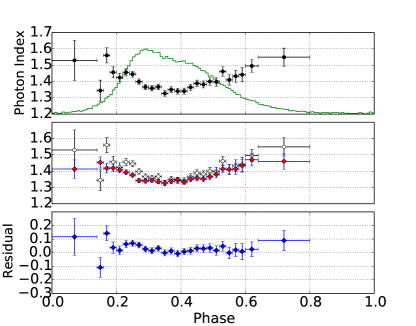
Figure 5.— Phase-resolved and pulsed spectral fits with the power law model. Top panel: photon indices of PSR B1509$-$58 at different phase ranges (black filled circles). The green line illustrates the pulse profile. Middle: comparison of the photon indices obtained in this paper (open black circles) with those of Ge et al (red filled diamonds). Bottom: difference between the photon indices obtained in this paper and in Ge et al. (2012).

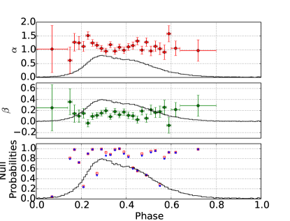
Figure 6.— Phase-resolved and pulsed spectral fits with the logpar model (Equation 1). The black line in each panels shows the pulse profile. Top panel: The parameter $\alpha$ as a function of phase. Middle: The parameter $\beta$ as a function of phase. Bottom: Null hypothesis probabilities obtained from $\chi^{2}$ tests for the power-law model (red open squares) and the logpar model (blue open stars). Many of them are very close to each other.

4. Discussion

We have reported on a pulsed spectral analysis and timing analysis of PSR B1509$-$58 with observations made by NuSTAR and Chandra, as well as previous results measured by COMPTEL and AGILE. The phase-averaged and pulsed spectral analysis shows that a smooth logarithmic parabolic model represents our 3-79 keV NuSTAR data better than a simple power-law model (Fig. 3 and Table 3). In addition, the logpar model describes our broadband spectrum well from 3 keV up to 500 MeV (Fig. 4 and Table 4). The phase-resolved and pulsed spectral analysis shows that the photon indices in 26 phase intervals are consistent with the results of Ge et al. (2012) (Fig. 5 and Table 5). However, the logpar model does not describe our spectra significantly better than the power-law model in any of these phase intervals (Fig. 6). In the timing analysis, we found that the pulsed profiles in 14 energy bands between 3-79 keV show no significant differences (Fig. 1). We measured the pulsed fraction of PSR B1509$-$58 in the hard X-ray band for the first time (Fig. 2). The measured pulsed fraction increased from $\sim$0.68 to $\sim$0.88 from 3 to 19 keV because of the PWN contamination which is significant due to the broad NuSTAR PSF, and then reached a plateau near the latter value within 19–79 keV.

4.1. Pulsed and Phase-Averaged Spectrum

In comparison to the results of Cusumano et al. (2001) (Table 3), uncertainties in our parameters are 50%-75% smaller. To compare the shape of our logpar model to Cusumano’s, we fixed all parameters at Cusumano’s values but let the normalization factors vary, and fitted our NuSTAR data with this model in XSPEC with $\chi^{2}$ minimization. The results were not acceptable, with a probability smaller than 10^-8. Figure 7 compares Cusumano’s model to our logpar model, and to the NuSTAR data. The difference in shape is visible. Moreover, our pulsed flux at 2–10 keV is ($2.39\pm 0.04)\times 10^{-11}$ erg cm^-2 s^-1, significantly larger than the $2.0\times 10^{-11}$ erg cm^-2 s^-1 reported by Cusumano et al. (2001), but consistent with the $(2.30\pm 0.02)\times 10^{-11}$erg cm^-2 s^-1 reported by Ge et al. (2012), and the $(2.52\pm 0.05)\times 10^{-11}\rm erg\rm~{}cm^{-2}\rm~{}s^{-1}$ reported by Kuiper & Hermsen (2015). However, Cusumano’s results were determined from BeppoSAX observations. As argued in Section 1, we consider our NuSTAR results more reliable than the BeppoSAX results, as BeppoSAX had systematic cross-calibration discrepancies among its three instruments among different energy bands.

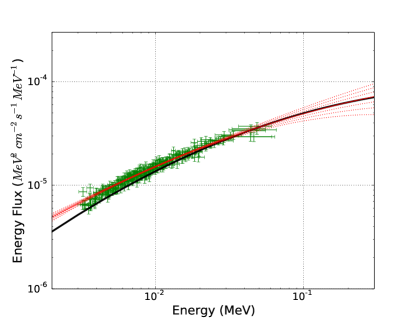
Figure 7.— Energy spectrum of our NuSTAR observation and that from Cusumano et al. (2001). The green points are NuSTAR data. The solid black curve is the result of Cusumano et al. (2001). The solid red curve is the NuSTAR logpar spectral model, and the dotted curves are its 1, 2 and 3$\sigma$ ranges.

We also compared the results of our observations with previous X-ray observations and summarize the comparison in Table 6. A simple extrapolation of the observation results of OSSE (50 keV–5 MeV), Ginga (3–60 keV), RXTE (2–250 keV) and WELCOME (94–240 keV) into our energy range predicts a pulsed flux of $\sim$1.26$\times 10^{-10}$, $\sim$1.50$\times 10^{-10}$, $\sim$2.20$\times 10^{-10}$ and $\sim$3.14$\times 10^{-10}$ erg cm^-2 s^-1, respectively. The pulsed fluxes predicted by OSSE and Ginga are consistent with our NuSTAR flux in 3–79 keV, while RXTE and WELCOME each predict a pulsed flux of $\sim$2 and $\sim$3 times larger than our NuSTAR flux. Note that cross-calibration discrepancies among NuSTAR, Ginga and RXTE against the Crab nebula have been found. NuSTAR was reported to measure the Crab spectrum $\sim$15% lower than Ginga and RXTE (Madsen et al. 2015; Kirsch et al. 2005). Also NuSTAR has an uncertainty of $\sim$5% on its absolute flux measurement, and the Crab flux could change by a few percent per year (Wilson-Hodge et al. 2011). Furthermore, the Ginga (3–60 keV), RXTE (2–250 keV), WELCOME (94–240 keV) and OSSE (50 keV–5 MeV) observations were reported to fit with simple power-law models. Their photon indices were $1.30\pm 0.05$ (Ginga; Kawai et al. 1993), $1.358\pm 0.014$ (RXTE; Marsden et al. 1997), $1.64^{+0.43}_{-0.42}$ (WELCOME; Gunji et al. 1994) and $1.68\pm 0.09$ (OSSE; Matz et al. 1994) (Table 6). This indicates that the pulsed spectrum becomes softer as energy increases, consistent with the behavior of our logpar model.

Table 6Predicted pulsed flux

Observation	Energy band	Photon Index	Flux in 3–79 keV
	[keV]		[10-10erg cm-2 s-1]
NuSTAR	3–79	$1.386\pm 0.007$	$1.136\pm 0.018$
Ginga	3–60	$1.30\pm 0.05$	$\sim$1.50
RXTE	2–250	$1.358\pm 0.014$	$\sim$2.20
WELCOME	94–240	$1.64^{+0.43}_{-0.42}$	$\sim$3.14
OSSE	50–5000	$1.68\pm 0.09$	$\sim$1.26

Figure 8 shows a comparison of the best-fit energy spectrum from our NuSTAR observations with those of the four previous X-ray observations. OSSE is within 3$\sigma$ from our NuSTAR spectrum, while RXTE, WELCOME and Ginga do not agree well with our new NuSTAR measurements. This perhaps is due to the cross-calibration issues between instruments described earlier in this section, since the source flux has been very stable over a long period (Livingstone & Kaspi 2011). Note that the uncertainty of the model increases dramatically with energy.

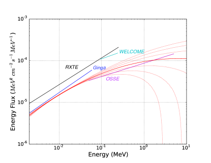
Figure 8.— Energy spectrum of NuSTAR data and previous X-ray observations. The solid red line is the NuSTAR logpar spectral model, and the dotted red lines are its 1, 2 and 3$\sigma$ ranges. The solid black line, solid cyan line, solid blue line, and solid magenta line, from top to bottom, are X-ray spectra observed by RXTE, WELCOME, Ginga and OSSE, respectively.

In their broadband spectral analysis, Cusumano et al. (2001) claimed that a smooth logarithmic parabolic model could represent the spectrum well up to 30 MeV, but must break more rapidly afterwards. However, our result shows that a logarithmic parabolic function can represent the spectrum well up to 500 MeV. Moreover, one interesting feature of the broadband energy spectrum is its peak energy. According to Equation 1, the energy flux should have a maximum at the following energy:

$$E_{m}=E_{0}10^{[(2-\alpha)/(2\beta)]},$$ (2)

which corresponds to 3 MeV and a 90% upper limit of 8 MeV, using the best-fit parameters obtained from NuSTAR alone, $4\pm 2$ MeV using the combined fit of NuSTAR and COMPTEL from 3 keV to 30 MeV, and $2.6\pm 0.8$ MeV using results obtained from all data up to 500 MeV. This value is consistent with the recent results of Kuiper & Hermsen (2015). Using multi-year data across $\sim$2 keV–1 GeV from RXTE PCA/HEXTE, Fermi LAT, COMPTEL and INTEGRAL ISGRI, they performed a broad-band spectral fit of the pulsed emission of PSR B1509$-$58 to a power-law model with a modified exponential cutoff, and derived a maximum luminosity per energy decade at $\sim$2.5 MeV. The result of Cusumano et al. (2001) was obtained from a combined fit of their BeppoSAX X-ray observation and COMPTEL, from 1 keV to 30 MeV. Their peak energy was 5 MeV, with a 90% upper limit of 14 MeV. Their value agrees with all of ours, though their uncertainty is $\sim$9 times larger than what we have obtained from the combined fit. Note that each of the $\gamma$-ray data points plays an important role in our combined fits, and in the determination of the peak value.

Cusumano et al. (2001) also discussed the relation of the peak values between PSR B1509$-$58 and the Crab pulsar. For the outer gap model, the synchrotron spectrum emitted from the secondary electron-positron pairs created by inward flowing curvature photons of Crab-like pulsars is predicted to obey the following scaling relation (Cusumano et al. 2001):

$$(E_{m}/E_{mC})\sim(P/P_{C})^{7/4}(\dot{P}/\dot{P_{C}})^{1/4}.$$ (3)

Here, $P_{C}$ and $\dot{P_{C}}$ are period and spin-down rate of the Crab, $E_{m}$, $E_{mC}$ are energies corresponding to the spectral peaks of the Crab-like pulsar and the Crab. It is suggested that a Crab-like pulsar spectrum that follows this relation is likely to be synchrotron radiation from the secondary pairs (Cusumano et al. 2001). For PSR B1509$-$58, the RHS of Equation 3 is $\sim$20. For the Crab, the SED peak energy ($E_{mC}$) is $\sim$14 keV for the main pulse, and $\sim$200 keV for the interpulse component. Cusumano et al. (2001) concluded that their observation agreed with this ratio when the spectrum of the Crab’s interpulse region was considered, but it was about one order of magnitude larger than the result when the spectrum of the Crab’s main pulse was considered. We can improve on this result thanks to our more precisely measured peak energy. From our analysis, the peak value obtained from our combined fit (3 keV–500 MeV) gives a ratio of $\sim$$5\pm 2$ when considering the Crab’s interpulse region, and $\sim$$80\pm 20$ for the Crab’s main pulse. Neither agrees well with the ratio of $\sim$20 predicted by Equation 3. Note that the exact uncertainties of $E_{mC}$ or the RHS of Equation 3 are unavailable to us, so the conclusion is based on estimations.

4.2. Predicted Spectra from Theoretical Models

PSR B1509$-$58 has an atypical spectrum in the X-ray and $\gamma$-ray bands. $\gamma$-ray pulsars typically have spectral peaks in the GeV energy band (Thompson 2004), while PSR B1509$-$58 was observed to emit very little $\gamma$-ray emission, and its energy spectrum peaks in the hard X-ray band at $2.6\pm 0.8$ MeV (Section 3.3). Wang et al. (2013) proposed a model in the context of outer gap acceleration to explain the weak $\gamma$-ray emission from this pulsar and calculated the X-ray spectrum. They proposed that the outgoing GeV–band $\gamma$-ray radiated via curvature radiation from the electron-positron pairs created in the null charge surface are missed because of the Earth viewing angle, while the inward propagating $\gamma$-rays passing near the pulsar surface may be absorbed by the magnetic field and converted into electron-positron pairs. The secondary pairs that travel with sufficiently large pitch angles with respect to the magnetic field lines emit synchrotron radiation which peaks at $\sim$10 MeV, and covers a wider sky area compared with curvature radiation of the primary particles. They concluded that only synchrotron radiation could be observed due to our viewing angles. However, the model may under-predict emissions in the X-ray band. For example, Wang et al. (2013) compared the energy spectrum predicted by their model with previous X-ray observations by Ginga, OSSE, WELCOME and RXTE, and found that the model predicts lower energy flux than is seen in all these observations except that of OSSE. The predicted energy flux is $\sim$half as much as observed by RXTE and WELCOME, and more than 5$\sigma$ lower than the RXTE observation.

We quantitatively compared our results with the theoretical model prediction that was shown in Figure 6 of Wang et al. (2013). By inspection, their theoretical prediction is roughly consistent with our NuSTAR 3$\sigma$ ranges (Fig. 8). Moreover, the theoretical model predicts a peak at $\sim$3 MeV (Wang et al. 2013), which agrees with our results.

4.3. Pulsed and Phase-resolved Spectrum

We also studied the pulsed, phase-resolved spectrum of PSR B1509$-$58. We found that the photon index is $1.34\pm 0.02$ in the middle of the pulse, becoming larger at the two sides, for the power-law model. Our results are largely consistent with those of Ge et al. (2012). Note that in 24 phases our photon indices are slightly larger than those of Ge et al. (2012) (see Fig. 5, middle and bottom panels). This may be consistent with the fact that the photon index increases with energy in the X-ray band, since our results were obtained from NuSTAR between 3–79 keV, higher than their 3–30 keV energy band.

Ge et al. (2012) performed pulsed and phase-resolved spectral analyses for three young and bright X-ray pulsars: the Crab pulsar, PSR B1509$-$58 and PSR B0540$-$69. Their results show that the photon indices of PSRs B1509$-$58 and B0540$-$69 are harder at the centres of the pulse profiles and softer at the wings, while those of the Crab pulsar are softer at its two peaks. However, their timing analysis shows that the pulse profiles of PSRs B1509$-$58 and B0540$-$69 could each be further decomposed into two narrower Gaussian components. Taking this into account, they concluded that overall the three pulsars’ photon indices had a similar evolving trend with their pulsed flux. Our NuSTAR observations support the same conclusion.

4.4. Pulsed Fraction

Wang et al. (2013)’s model clearly predicted X-ray off-pulse emission from the pulsar, and those authors suggested that it was probably produced by electrons accelerated transverse to the field line. We have measured the pulsed fraction of PSR B1509$-$58 with NuSTAR in the 3–79 keV band and with Chandra HRC in the 0.5–10 keV band. The observed off-pulse emission originated from both the pulsar and the PWN. With our pulsed fraction measurements, we can determine the contributions from the PWN and the PWN-free pulsar off-pulse components to the total emission, and estimate the photon index of the pulsar’s off-pulse component for the first time.

Based on the results shown in Figure 2, we had that at 3-4 keV, the PWN-free pulsed fraction measured with Chandra is:

$$PF_{\rm PWN-free}=\frac{pulsed}{pulsed+offpulse_{\rm PWN-free}}=0.88\pm 0.06,$$

while the PWN-included result from NuSTAR is:

$$\begin{split}PF_{\rm withPWN}&=\frac{pulsed}{pulsed+{offpulse}_{\rm PWN-free}+PWN}\\ &=0.68\pm 0.04.\end{split}$$

From these two results, we derived that the PWN contrioff-pulsebutes $0.23\pm 0.06$ of the total number of NuSTAR photons, and that the pulsar’s PWN-free off-pulse component contributes $0.09\pm 0.07$ of the total number of photons. The latter result is roughly consistent with what is shown in Figure 2, where the pulsed fraction approaches 90%. The number of photons detected from the PWN is $3\pm 2$ times of those from the pulsar’s PWN-free off-pulse component at $\sim$3–4 keV. Consequently, the pulse-off components at soft X-ray bands are likely to be PWN-dominated, and as energy increases the PWN contribution decreases until $\sim$19 keV, where it no longer matters. The off-pulse components of 19–79 keV are composed of the pulsar’s PWN-free off-pulse component alone.

Additionally, we can estimate the photon index of the pulsar’s PWN-free off-pulse component. The PWN spectrum is much softer than the pulsar’s: the photon indices of the PWN and the pulsar are 1.6–1.8 (An et al. 2014) and $1.386\pm 0.007$, respectively. The PWN is also much fainter than the pulsar: at 19 keV, its flux is less than 1% of the pulsar’s. Hence we can safely neglect the PWN contribution above 19 keV and regard the NuSTAR results between 19–25 keV and 25–79 keV as PWN-free pulsed fractions of the pulsar. Meanwhile, the Chandra HRC results also give the PWN-free pulsed fraction. Figure 2 shows that the four PWN-free pulsed fractions, namely the two NuSTAR results in 19–25 keV and 25–79 keV, as well as the two Chandra results within 0.5–10 keV, are consistent. Assuming that the PWN-free off-pulse components is well represented by a simple power-law model, the PWN-free pulsed fraction is then

$$PF=\frac{KE^{-\alpha-\beta log(\frac{E}{E_{\rm p}})}}{KE^{-\alpha-\beta log(\frac{E}{E_{\rm p}})}+K_{off-pulse}E^{-\Gamma}}.$$ (4)

Here $K_{off-pulse}$ and $\Gamma$ are the normalization factor and the photon index of the pulsar’s PWN-free off-pulse component, to be determined. $K$, $\alpha$ and $\beta$ are the same as in Equation 1 and Table 3. With these four PWN-free pulsed fraction results, we took their upper and lower 1$\sigma$ limits and estimated that the off-pulse component’s photon index is between 1.26 and 1.96. This constraint is weak due to the large uncertainties. NuSTAR observations with longer exposure time could be useful for constraining the off-pulse spectrum better.

5. Summary

We have presented NuSTAR hard X-ray observations of the young rotation-powered radio pulsar PSR B1509$-$58 in the supernova remnant MSH 15$-$52. We have confirmed the curvature in the hard X-ray band reported by Cusumano et al. (2001), and have showed that the logpar model is statistically a better representation of our spectrum in both the NuSTAR energy band from 3 to 79 keV, and a broadband from 3 keV to 500 MeV. The logpar model predicts that the broadband energy spectrum peaks at $2.6\pm 0.8$ MeV, $\sim$9 times more precisely determined than before, and consistent with the recent result of Kuiper & Hermsen (2015). We have also fitted the logpar model and the power-law model to the phase-resolved spectra in 26 phase intervals, but found that statistically the logpar model was not significantly superior to the power-law model in any of these phase intervals. In addition, we have measured the pulsed fraction of PSR B1509$-$58 in the hard X-ray energy band for the first time. The results imply that the PWN contributes $0.23\pm 0.06$ of the total number of NuSTAR photons, while the pulsar’s PWN-free off-pulse component contributes $0.09\pm 0.07$ of the total number of photons. We have also estimated that the off-pulse component’s photon index is between 1.26 and 1.96. To improve the constraint, NuSTAR observations with longer exposure time could be helpful. Finally, these new NuSTAR observations support a model (Wang et al. 2013) in which the X-rays originate from secondary pairs producing synchrotron radiation. The model describes how outgoing GeV emission goes undetected because of the Earth viewing angle. This helps to understand PSR B1509$-58$’s lack of GeV emission, and provides a possible answer to the long-lasting question about the source’s atypical spectrum.

This work was supported under NASA Contract No. NNG08FD60C, and made use of data from the NuSTAR mission, a project led by the California Institute of Technology, managed by the Jet Propulsion Laboratory, and funded by the National Aeronautics and Space Administration. We thank the NuSTAR Operations, Software and Calibration teams for support with the execution and analysis of these observations. This research has made use of the NuSTAR Data Analysis Software (NuSTARDAS) jointly developed by the ASI Science Data Center (ASDC, Italy) and the California Institute of Technology (USA). H.A. acknowledges supports provided by the NASA sponsored Fermi Contract NAS5-00147 and by Kavli Institute for Particle Astrophysics and Cosmology. V.M.K. acknowledges support from an NSERC Discovery Grant and Accelerator Supplement, the FQRNT Centre de Recherche Astrophysique du Quebec, an R. Howard Webster Foundation Fellowship from the Canadian Institute for Advanced Research (CIFAR), the Canada Research Chairs Program and the Lorne Trottier Chair in Astrophysics and Cosmology.

References

- Abdo et al. (2010) Abdo, A. A., Ackermann, M., Ajello, M., et al. 2010, ApJ, 714, 927
- An et al. (2014) An, H., Madsen, K. K., Reynolds, S. P., et al. 2014, The Astrophysical Journal, 793, 90
- Barlow (1989) Barlow, R. J. 1989, Statistics: A Guide to the Use of Statistical Methods in the Physical Sciences (Manchester Physics Series), reprint edn. (WileyBlackwell)
- Boella et al. (1997) Boella, G., Butler, R. C., Perola, G. C., et al. 1997, A&AS, 122, 299
- Cusumano et al. (2001) Cusumano, G., Mineo, T., Massaro, E., et al. 2001, A&A, 375, 397
- Dib et al. (2009) Dib, R., Kaspi, V. M., & Gavriil, F. P. 2009, The Astrophysical Journal, 702, 614
- Ge et al. (2012) Ge, M. Y., Lu, F. J., Qu, J. L., et al. 2012, ApJS, 199, 32
- Gunji et al. (1994) Gunji, S., Hirayama, M., Kamae, T., et al. 1994, ApJ, 428, 284
- Harrison et al. (2013) Harrison, F. A., Craig, W. W., Christensen, F. E., et al. 2013, ApJ, 770, 103
- Kawai et al. (1993) Kawai, N., Okayasu, R., & Sekimoto, Y. 1993, in American Institute of Physics Conference Series, Vol. 280, American Institute of Physics Conference Series, ed. M. Friedlander, N. Gehrels, & D. J. Macomb, 213–217
- Kirsch et al. (2005) Kirsch, M. G., Briel, U. G., Burrows, D., et al. 2005, in Society of Photo-Optical Instrumentation Engineers (SPIE) Conference Series, Vol. 5898, UV, X-Ray, and Gamma-Ray Space Instrumentation for Astronomy XIV, ed. O. H. W. Siegmund, 22–33
- Kuiper & Hermsen (2015) Kuiper, L., & Hermsen, W. 2015, MNRAS, 449, 3827
- Kuiper et al. (1999) Kuiper, L., Hermsen, W., Krijger, J. M., et al. 1999, A&A, 351, 119
- Livingstone & Kaspi (2011) Livingstone, M. A., & Kaspi, V. M. 2011, ApJ, 742, 31
- Madsen et al. (2015) Madsen, K. K., Harrison, F. A., Markwardt, C., et al. 2015, arXiv preprint arXiv:1504.01672
- Manchester et al. (1982) Manchester, R. N., Tuohy, I. R., & Damico, N. 1982, ApJ, 262, L31
- Marsden et al. (1997) Marsden, D., Blanco, P., Gruber, D., et al. 1997, The Astrophysical Journal Letters, 491, L39
- Matz et al. (1994) Matz, S., Ulmer, M. P., Grabelsky, D. A., et al. 1994, ApJ, 434, 288
- Orlandini et al. (2012) Orlandini, M., Frontera, F., Masetti, N., Sguera, V., & Sidoli, L. 2012, ApJ, 748, 86
- Pilia et al. (2010) Pilia, M., Pellizzoni, A., Trois, A., et al. 2010, ApJ, 723, 707
- Rea et al. (2013) Rea, N., Israel, G. L., Pons, J. A., et al. 2013, ApJ, 770, 65
- Seward & Harnden (1982) Seward, F. D., & Harnden, Jr., F. R. 1982, ApJ, 256, L45
- Tamura et al. (1996) Tamura, K., Kawai, N., Yoshida, A., & Brinkmann, W. 1996, PASJ, 48, L33
- Thompson (2004) Thompson, D. J. 2004, in Astrophysics and Space Science Library, Vol. 304, Cosmic Gamma-Ray Sources, ed. K. S. Cheng & G. E. Romero, 149
- Wang et al. (2013) Wang, Y., Takata, J., & Cheng, K. S. 2013, The Astrophysical Journal, 764, 51
- Wilson-Hodge et al. (2011) Wilson-Hodge, C. A., Cherry, M. L., Case, G. L., et al. 2011, The Astrophysical Journal Letters, 727, L40