Moving contact line dynamics: from diffuse to sharp interfaces

Abstract

We reconcile two scaling laws that have been proposed in the literature for the slip length associated with a moving contact line in diffuse interface models, by demonstrating each to apply in a different regime of the ratio of the microscopic interfacial width $l$ and the macroscopic diffusive length $l_{D}=(M\eta)^{1/2}$, where $\eta$ is the fluid viscosity and $M$ the mobility governing intermolecular diffusion. For small $l_{D}/l$ we find a diffuse interface regime in which the slip length scales as $\xi\sim(l_{D}l)^{1/2}$. For larger $l_{D}/l>1$ we find a sharp interface regime in which the slip length depends only on the diffusive length, $\xi\sim l_{D}\sim(M\eta)^{1/2}$, and therefore only on the macroscopic variables $\eta$ and $M$, independent of the microscopic interfacial width $l$. We also give evidence that modifying the microscopic interfacial terms in the model’s free energy functional appears to affect the value of the slip length only in the diffuse interface regime, consistent with the slip length depending only on macroscopic variables in the sharp interface regime. Finally, we demonstrate the dependence of the dynamic contact angle on the capillary number to be in excellent agreement with the theoretical prediction of Cox (1986), provided we allow the slip length to be rescaled by a dimensionless prefactor. This prefactor appears to converge to unity in the sharp interface limit, but is smaller in the diffuse interface limit. The excellent agreement of results obtained using three independent numerical methods, across several decades of the relevant dimensionless variables, demonstrates our findings to be free of numerical artifacts.

I Introduction

Understanding the way in which a contact line (the line along which an interface separating two immiscible fluids intersects a solid boundary wall) moves under an imposed flow is a problem of fundamental importance in wetting dynamics. It underpins a wide range of phenomena in nature, for example in the functional adaptation of many biological systems (Parker and Lawrence, 2001; Zheng et al., 2007; Hu et al., 2003), as well as in technological applications: from oil recovery (Morrow, 1990) to inkjet printing and microfluidics (Tabeling, 2010). From these examples, it has become clear that experimental progress needs to be accompanied by the development of physical models and computational methods that can accurately capture wetting dynamics, even in complex geometries.

Any purely macroscopic treatment – in which the two fluids are considered to be separated by a strictly sharp interface, and subject to a strictly no-slip condition on the fluid-velocity at the solid wall – has long been recognised to predict a non-integrable stress singularity for any non-zero velocity of the contact line  (Huh and Scriven, 1971; de Gennes, 1985). This so-called moving contact line singularity is clearly at odds with the commonplace experience that the contact line does, in fact, move.

To regularise this singularity, the macroscopic picture just described must be supplemented by additional physics that intervenes on shorter, microscopic lengthscales. One approach is to relax the no-slip boundary condition on the fluid velocity, by inserting a slip boundary condition in a region of microscopic size $\xi$ in the vicinity of the contact line. This can be done by hand (Zhou and Sheng, 1990; Spelt, 2005), for example by imposing a slip velocity $v_{\rm s}=U\exp(-|x|/\xi)$, where $x$ is the distance along the wall away from the contact line, or by choosing $v_{\rm s}=\xi\sigma/\eta$, where $\sigma$ and $\eta$ are the wall stress and fluid viscosity respectively. In any computational study, slip can also arise indirectly as a numerical artifact (Renardy et al., 2001).

Another approach is to keep the no-slip boundary condition and instead to recognise that any interface between two fluids can never be perfectly sharp, but in practice must have some non-zero microscopic diffuse width $l$. Accordingly, the use of diffusive interface models (Anderson et al., 1998; Jacqmin, 2000) has gained increasing popularity in recent years. A diffuse interface model of liquid-gas coexistence then accommodates contact line motion by a condensation-evaporation mechanism which, in some small region within close proximity of the contact line, slowly transfers matter from one side of the interface to the other (Seppecher, 1996; Briant et al., 2004; Pooley et al., 2009; Diotallevi et al., 2009). Similarly, a diffuse interface model of coexisting immiscible binary fluids accommodates contact line motion via a slow intermolecular diffusion of the two fluids across the interface between them, again acting in a small region in the vicinity of the contact line (Jacqmin, 2000; Briant and Yeomans, 2004; Pooley et al., 2009).

Diffuse interface models (Anderson et al., 1998; Jacqmin, 2000) are also convenient in computational practice. An order parameter (“phase field”) is introduced to distinguish one fluid from another, with the length scale that characterises the variation of this field across the interface between the fluids prescribing the interfacial width, $l$. An advection-diffusion equation (the Cahn-Hilliard equation supplemented by an advective term) then determines the evolution of this order parameter, and hence of the interface position. This is solved in tandem with the Navier-Stokes equation for the fluid velocity field. A key advantage of this approach is that all computational grid points are treated on an equal footing, without any need to explicitly track the position of the interface. In this way, even complex flow geometries can be simulated conveniently.

It is important to emphasize, as first elucidated by  Cox (1986), that although the physical origins of contact line motion may differ according to the detailed microscopic physics invoked (wall slip, intermolecular diffusion across the interface, etc.), the macroscopic hydrodynamics far from the contact line nonetheless converges to a universal solution that is informed by the microscopics only in the sense of being rescaled by a single parameter, the “slip length” $\xi$, that emerges from this underlying microscopic physics. An important problem within any model of the microscopics is therefore to determine this emergent slip length $\xi$: not only because it is a key variable that determines the macroscopic wetting and fluid dynamics, but also because it sets a scale to which other length scales (surface heterogeneities, droplet size, etc.) must be compared.

With that motivation in mind, the primary aim of this work is to determine the scaling of the slip length within a diffuse interface model of immiscible binary fluids. We assume the fluids to have matched viscosity $\eta$, and denote by $M$ the mobility parameter characterising the rate of intermolecular diffusion in the Cahn-Hilliard equation. In the existing literature, (at least) three apparently contradictory scalings have been proposed. Several authors (e.g. Jacqmin (2000), Yue et al. (2010)) suggest that $\xi\sim l_{D}$ where $l_{D}=(M\eta)^{1/2}$ is the characteristic lengthscale below which intermolecular diffusion dominates advection and above which the opposite is true. For convenience we call this the diffusion length in what follows, and we emphasise that it is determined only by the macroscopic quantities $M$ and $\eta$. In contrast, Briant and Yeomans (2004) suggest a different scaling, $\xi\sim\sqrt{l_{D}l}$, which is the geometric mean of the macroscopic diffusion length and the microscopic interface width. And while these two proposed scalings do not have any dependence on the imposed flow velocity, Chen et al. (2000) in contrast suggested that the slip length does depend on the velocity as $\xi\propto V_{0}^{-1/2}$.

In view of these apparently contradictory predictions, an important contribution of this work is to provide a coherent picture that fully reconciles two of these existing predictions, by showing each to apply in a different regime of parameter space, and that carefully appraises the third. This is achieved by extensive numerical studies performed across unprecedently wide ranges of the two relevant control parameters. Specifically, we explore four decades of the dimensionless ratio $M\eta/l^{2}=l_{D}^{2}/l^{2}$ of the (squared) macroscopic diffusion length to the (squared) microscopic interface width; and three decades of the capillary number Ca (defined below), which adimensionalises the imposed flow velocity $V_{0}$ in terms of an intrinsic interfacial velocity scale. Moreover we use three different, independently coded numerical methods, and show their results to be in excellent quantitative agreement across all decades.

For small values of the capillary number Ca, corresponding to low imposed flow velocities, we demonstrate that the slip length converges to a well-defined value that is independent of the velocity $V_{0}$. Any dependence on the velocity is only observed for $\mbox{{Ca}}>0.01$, and we comment on the extent to which our results are consistent with the prediction $\xi\propto V_{0}^{-1/2}$ of Chen et al. (2000) in this fast flowing regime.

The remainder of the paper focuses on the slow flow regime, $\mbox{{Ca}}<0.01$, in which the slip length $\xi$ is independent of the flow rate $V_{0}$. Here we show that, in the limit of large $l_{D}/l$, the slip length scales as $\xi\propto l_{D}$, informed only by the macroscopic lengthscale $l_{D}$. This agrees with the original prediction of Jacqmin (2000), Yue et al. (2010) and corresponds to the sharp interface limit of the diffuse interface model. In this limit the microscopic length $l$ essentially drops out of the problem, apart from providing a “singular perturbation” to regularise the contact line singularity. In contrast, for small $l_{D}/l$ we find that the slip length scales as $\xi\propto(l_{D}l)^{1/2}$, as proposed by Briant and Yeomans (2004). This corresponds to the diffuse interface limit in which the emergent slip length does depend on the underlying microscopic length $l$. In this way we reconcile these two previously apparently contradictory scalings, by showing each to apply in a different limiting regime of $l_{D}/l$. The crossover between the two is furthermore consistent with the onset of the sharp interface regime discussed by Yue et al. (2010).

The fact that the slip length $\xi$ is in general different from the interface width $l$, and indeed greatly exceeds it for large $l_{D}/l$, has a clear practical consequence for any simulation: the resolution of the full wetting dynamics appears only on a lengthscale corresponding to the larger of the interface width and the slip length. This, in turn, limits the region of parameter space that can be considered reliable in any numerical study.

We provide additional evidence for the distinction between the diffuse interface limit $l_{D}/l\ll 1$, in which the microscopic physics informs $\xi$, and the sharp interface limit $l_{D}/l\gg 1$, in which it does not, by performing further simulations in which the we modify the interfacial (microscopic) contribution to the underlying free energy functional of the binary fluid. We show that the slip length depends on this modification only in the diffuse interface regime. In the sharp interface regime of large $l_{D}/l$, the slip length continues to depend only on the macroscopic dynamical variables, $\eta$ and $M$, free of this modification to the microscopic interfacial term.

Finally, we test the validity of Cox’s formula (Cox, 1986) for the dependence of the dynamic contact angle on the Capillary number in the different slip length regimes. Our numerical results are in good agreement with Cox’s analytical result if we allow the slip length to be rescaled by a dimensionless parameter. Moreover this parameter appears, suggestively, to converge to unity in the sharp interface limit, but is smaller in the diffuse interface limit.

This paper is organized as follows. In the next section we describe the models, methods and setups we employ to compute the slip lengths and dynamic contact angles. We present our results in section IV. Finally, we summarise our key findings and discuss avenues for further work in section V.

II Model, geometry and boundary conditions

In this section we specify the model that we shall use throughout the paper, starting with the thermodynamics in Secs. II.1 and II.2 then the dynamical equations of motion in Sec. II.3. We then specify the flow geometry and boundary conditions in Sec. II.4.

II.1 Thermodynamics

We consider a binary mixture of two mutually phobic fluids, $A$ and $B$, and denote the volume fraction of fluid $A$ by the continuum phase field $\phi(\mathbf{r},t)$. The volume fraction of fluid $B$ is then simply 1-$\phi$ by mass conservation and need not be considered separately. We consider a Landau free energy (Bray, 1994)

$$\Psi=\int_{V}\psi_{b}\,\,dV=\int_{V}\left[\frac{G}{4}(\phi^{2}-1)^{2}+\frac{Gl^{2}}{2}(\nabla\phi)^{2}\right]dV,$$ (1)

which allows a coexistence of two bulk phases: an A-rich phase with $\phi_{A}=1$ and a B-rich phase with $\phi_{B}=-1$. The bulk constant $G$ has dimensions of energy per unit volume (or equivalently of force per unit area, and so modulus). If the two fluids have different affinities to the solid surface, a surface (wetting) contribution to the free energy can be added (Cahn, 1977; Pooley et al., 2008, 2009) to the right hand side of Eq. (1). Throughout this work we assume neutral wetting conditions, for which no such contribution is needed.

The chemical potential $\mu$ follows as a functional derivative of the free energy density $\psi_{b}$ with respect to $\phi$, giving

$$\mu=-G\phi+G\phi^{3}-Gl^{2}\,\nabla^{2}\phi.$$ (2)

In equilibrium the chemical potential $\mu=0$. Assuming a flat interface of infinite extent in the $y-z$ plane, with the interfacial normal in the $x$ direction and the interface located at $x=0$, we then obtain an interfacial solution of the form

$$\phi=\tanh\left(\frac{x}{\sqrt{2}l}\right),$$ (3)

with a homogeneous B-rich phase for $x\ll-l$ and homogeneous A-rich phase for $x\gg l$. The interfacial constant $l$ specifies the characteristic length scale over which $\phi$ varies in between these two phases, and so corresponds to the interfacial width. The surface tension associated with this interface is given by

$$\sigma=\frac{2\sqrt{2}Gl}{3}.$$ (4)

II.2 Generalisation of the Landau Theory: Introduction of a curvature term

So far, we have specified the Landau free energy in the form most commonly used in the literature. It will also be instructive in what follows to consider the extent to which our results for the slip length do or don’t depend on the microscopic details of the model used. Accordingly, we now generalise the free energy slightly to give

$$\Psi^{\prime}=\int_{V}\psi^{\prime}_{b}\,\,dV=\int_{V}\left[\frac{G}{4}(\phi^{2}-1)^{2}+\frac{Gl^{2}}{2}(\nabla\phi)^{2}+\alpha\frac{Gl^{4}}{4}(\nabla^{2}\phi)^{2}\right]dV.$$ (5)

Compared to the original free energy defined above, this has an additional interfacial curvature term of amplitude set by $\alpha$. The mapping between this form of Landau free energy and the (Helfrich) continuum elastic energy can be found in e.g. Gompper and Zschocke (1991). The associated chemical potential is

$$\mu=G\left(-\phi+\phi^{3}-l^{2}\,\nabla^{2}\phi-\alpha l^{4}\,\nabla^{4}\phi\right).$$ (6)

It is important to note that the bulk terms are unaltered, with the modification affecting only interfacial gradient terms involving powers of $l\,\nabla$. A careful comparison of the original model, for which $\alpha=0$, with this generalised model, for which $\alpha>0$, will allow us to demonstrate that the slip length is independent of the microscopic details, as specified by $\alpha$, in the sharp interface regime $l_{D}/l\gg 1$. In contrast in the diffuse interface regime $l_{D}/l\ll 1$ we find that the slip length does depend on the microscopics, via $\alpha$.

II.3 Equations of Motion

The dynamics of the order parameter field is specified by the Cahn-Hilliard equation (see e.g.  Bray, 1994) generalised to include an advective term:

$$\left(\partial_{t}+\mathbf{v}.\nabla\right)\phi=M\nabla^{2}\mu.$$ (7)

Here $M$ is the molecular mobility, which we assume constant. The fluid velocity and pressure fields, $\mathbf{v}(\mathbf{r},t)$ and $p(\mathbf{r},t)$, obey the continuity and Navier-Stokes equations

$$\partial_{t}\rho+\mathbf{v}.\nabla\rho=-\rho\nabla.\mathbf{v},$$ (8)

$$\rho\left(\partial_{t}+\mathbf{v}.\nabla\right)\mathbf{v}=\eta\nabla^{2}\mathbf{v}-\nabla p-\phi\nabla\mu.$$ (9)

We denote by $\rho$ and $\eta$ the fluid density and viscosity respectively, assuming throughout that the two fluids are perfectly matched in both density and viscosity. In the Navier-Stokes equation, gradients in the chemical potential contribute an additional forcing term to the fluid motion, $-\phi\nabla\mu$ (Jacqmin, 1999).

Diffuse interface models are widely used in the computational fluid dynamics community and they have been implemented using various approaches. To ensure our results are free from numerical artefacts, here we have used three different numerical methods: (MI) the lattice Boltzmann method, (MII) spectral method, and (MIII) immersed boundary method to solve the equations of motion. They are detailed in Sec. III below. For MII and MIII, we have assumed incompressible flow and taken the inertialess limit of zero Reynolds number Stokes flow. This corresponds to setting to zero the terms on the left-hand-sides of Eqn. 8 (incompressibility) and Eq. 9 (zero inertia). The Lattice-Boltzmann method (MI) intrinsically requires a small but non-zero inertia and compressibility, though our numerical results confirm the effects of this difference to be negligible for the problem considered here.

II.4 Geometry, initialisation and boundary conditions

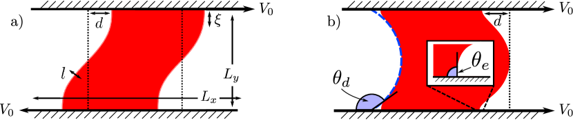
Figure 1: Schematic illustration of typical steady-states in our channel geometry. Marked are the key lengthscales: slip-length $\xi$, interface displacement $d$, channel dimensions $L_{x},L_{y}$, and diffuse interface width $l$. In panel a) a shear flow is imposed by moving the plates with equal and opposite velocities $\pm V_{0}$. In panel b) a Poiseuille flow is imposed by applying a pressure drop along the length of the channel, sketched here in the frame in which the fluid bridge is stationary. The definitions for the dynamic ($\theta_{d}$, macroscopic) and equilibrium ($\theta_{e}$, microscopic) contact angles are shown.

We consider flow between infinite flat parallel plates a distance $L_{y}$ apart, with plate normals in the $y$ direction. In the flow direction $x$ the cell is taken to have length $L_{x}=2L_{y}$, with periodic boundary conditions on both $\phi$ and $\mathbf{v}$. All quantities are assumed invariant in the $z$ direction. The phase field is initialised in an equilibrium state with a bridge of A-rich phase, in which $\phi=+1$, separated by two vertical diffuse interfaces of width $\ell$ at $x=L_{x}/4$ and $3L_{x}/4$ from B-rich phases on either side, where $\phi=-1$. The equilibrium contact angle is taken to be $\theta_{e}=90^{\circ}$, corresponding to neutral wetting conditions. Throughout we define the position of the interface itself by the locus $\phi=0$.

The fluid is taken to be initially at rest with $\mathbf{v}=0$ everywhere. Starting from this initial condition, we then implement one of two common flow protocols: boundary-driven planar Couette flow and pressure-driven planar Poiseuille flow. In the first of these, a constant shear-rate ${\dot{\gamma}}$ is applied by moving the top and bottom plates at velocities $V_{0}=\pm\frac{1}{2}{\dot{\gamma}}L_{y}$. This deforms the phase field and for small $\mbox{{Ca}}\equiv\eta V_{0}/\sigma\lesssim 0.1$ a steady state is reached in which the interface has displaced a distance $d\propto\pm\mbox{{Ca}}$ at the top and bottom walls, as shown in Fig. 1a. The deformed bridge is then stationary, with the contact lines moving at a velocity $\mp V_{0}$ relative to the top and bottom walls.

In the Poiseuille protocol the flow is driven by an imposed pressure drop $\Delta P$ along the length of the channel. A steady state then develops in which the bridge migrates along the channel at a constant speed, with the contact lines moving along each wall with a measured velocity $V_{0}$. In the reference frame of the contact line, therefore, both walls move with a velocity $-V_{0}$. By fitting the interface in the central region of the channel (between $y=\frac{1}{4}\to\frac{3}{4}$) to a circle, see Fig. 1b, we define the dynamic contact angle $\theta_{d}$ as the angle of intersection this circle makes with the wall. The dynamic contact angle is in general different from the equilibrium contact angle.

At the plates we assume boundary conditions of no-slip and no-permeation for the fluid velocity. For the phase field, we implement $\partial_{y}\mu|_{y=0,L_{y}}=0$ in method MIII. In method MII it is instead more convenient to set $\partial_{y}\phi|_{y=0,L_{y}}=\partial^{3}_{y}\phi|_{y=0,L_{y}}=\partial^{5}_{y}\phi|_{y=0,L_{y}}=0$ (where the last equality need only be imposed in the case $\alpha\neq 0$). Note that while this condition automatically ensures zero gradient of the chemical potential, it is actually a stronger condition than that in demanding all the relevant odd derivatives of $\phi$ to vanish separately. We do, however, find no difference in our numerical results between these. For method MI, the bounce-back boundary conditions assure we have no slip and no permeation of either fluid across the boundary.

II.5 Definition of the slip length

Our definition of the slip length uses the fact that the slip mechanism in the binary fluid model is intermolecular diffusion. In steady state, the Cahn-Hilliard equation of motion for the order parameter reads

$$\mathbf{v}.\nabla\phi=M\nabla^{2}\mu.$$ (10)

In Fig. 2, we plot the way in which $\mathbf{v}.\nabla\phi$ typically varies along the fluid-fluid interface (taken as the locus $\phi=0$, as noted above). We take the slip length $\xi$ to be given by the distance from the wall to the local maximum. In measuring this typical distance away from the wall over which $\mathbf{v}.\nabla\phi=M\nabla^{2}\mu$ remains appreciable, $\xi$ characterises the lengthscale over which intermolecular diffusion is important.

Other definitions of the slip lengths have been used in the literature to characterize the diffusive mechanism. For examples, Briant and Yeomans (2004) defined the slip length as the point at which $M\nabla^{2}\mu$ reaches -10% of the value at the wall after passing the first maximum, as measured along the interface; Yue et al. (2010) suggested the use of the location of the stagnation point in the flow. As we will show in the results section, we recover the same scaling laws for the diffuse and sharp interface limits as in Briant and Yeomans (2004) and Yue et al. (2010) respectively, strongly suggesting these definitions are not independent, as expected if there is a genuine characteristic length scale in the problem.

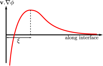
Figure 2: Illustration of our definition of the slip length $\xi$, defined as the position of the first local maximum of $\mathbf{v}.\nabla\phi$ as measured along the interface (defined as the locus $\phi=0$).

II.6 Parameters and dimensionless groups

For the model and flow geometry that we have now defined, we have the following parameters: the fluid density $\rho$, the fluid viscosity $\eta$, the modulus $G$ that sets the scale of the free energy density, the mobility $M$, the diffuse interfacial width $l$, the box dimensions $L_{x}$ and $L_{y}$, and the applied flow velocity $V_{0}$. (Also relevant numerically are the spatial mesh size and the timestep; we have ensured convergence for all the results presented.) As noted above, the fluid density is set to zero (inertialess flow) for methods MII and MIII, and small for MI. This leaves $\eta,G,M,l,L_{y},L_{x}$ and $V_{0}$ as the relevant parameters. We are then free to choose units of mass, length and time, thereby reducing by three the number of parameters that must be explored numerically. Accordingly, we work in what follows with the following dimensionless groups: $\sqrt{M\eta}/l$, $l/L_{y}$, $L_{x}/L_{y}$ and the capillary number $\mbox{{Ca}}=\eta V_{0}/\sigma$. The last of these characterises the speed of the imposed flow compared to the intrinsic interfacial velocity scale $\sigma/\eta$ formed by comparing the surface tension to the fluid viscosity (recall that the surface tension $\sigma\propto Gl$). Among these we set the aspect ratio of the box $L_{x}=2L_{y}$ throughout. The ratio $l/L_{y}$ is always set small, to ensure that the results are not contaminated by finite box size effects. This leaves $\sqrt{M\eta}/l$ and Ca as the two dimensionless groups to be explored numerically.

III Numerical Methods

In this section we describe our three numerical methods. For convenience we will refer to these throughout the manuscript as MI, MII and MIII. We emphasize that each was coded independently of the others, one by each of the authors of the manuscript, thereby providing confidence that our results are free of algorithmic artefacts.

III.1 Method I: Lattice Boltzmann Method

We use a standard free energy lattice Boltzmann method to solve the binary fluid equations of motion. The basic idea behind the lattice Boltzmann algorithm is to associate distribution functions, $\mathbf{f}({\bf r},t)=\{f_{i}({\bf r},t)\}$ and $\mathbf{g}({\bf r},t)=\{g_{i}({\bf r},t)\}$, discrete in time and space, to a set of velocity directions $\mathbf{e}_{i}$. Here we use a D2Q9 model, where $\mathbf{e}_{i}=(0,0),(\pm 1,0),(0,\pm 1),(\pm 1,\pm 1)$. The physical variables are related to the distribution functions by

$$\rho=\sum_{i}f_{i},\;\;\;\;\;\;\rho v_{\alpha}=\sum_{i}f_{i}e_{i\alpha},\;\;\;\;\;\;\phi=\sum_{i}g_{i},\;\;\;\;\;\;\phi v_{\alpha}=\sum_{i}g_{i}e_{i\alpha}.$$ (11)

The time evolution equations for the distribution functions can be broken down into two steps. In the collision step, we have used a single relaxation time approach for the order parameter and a multiple relaxation time approach for the fluid density,

$$\mathbf{f}^{\prime}({\bf r},t)=\mathbf{f}({\bf r},t)-\mathbf{M^{-1}SM}[\mathbf{f}({\bf r},t)-\mathbf{f}^{eq}({\bf r},t)]\,,$$

$$\mathbf{g}^{\prime}({\bf r},t)=\mathbf{g}({\bf r},t)-\frac{1}{\tau_{\phi}}\left[\mathbf{g}({\bf r},t)-\mathbf{g}^{eq}({\bf r},t)\right].$$ (12)

As shown by Pooley et al. (2008), the multiple relaxation time approach is significantly more reliable to reduce spurious velocities at the contact line. $\mathbf{f}^{eq}$ and $\mathbf{g}^{eq}$ are local equilibrium distribution functions. The choice of the local equilibrium functions must recover the correct thermodynamics and hydrodynamics equations of motion in the continuum limit. The matrix $\mathbf{M}$ performs a change of basis to more physically relevant variables, including the density, momentum, and viscous stress tensor. The matrix $\mathbf{S}$ is a diagonal matrix and contains the information about how fast each of these physical variables relaxes to equilibrium at every time step. Detailed expressions for $\mathbf{f}^{eq}$, $\mathbf{g}^{eq}$, $\mathbf{M}$, and $\mathbf{S}$ can be found in Pooley et al. (2008).

The relaxation parameter $\tau$ for the viscous stress tensor in $\mathbf{S}$ can be related to the kinematic shear viscosity $\nu=\eta/\rho$ via

$$\nu=(\Delta t(\tau-1/2))/3\,.$$ (13)

Similarly, the relaxation parameter $\tau_{\phi}$ for the order parameter is related to the mobility parameter in the Cahn-Hilliard equation through

$$M=\Delta t\Gamma\left(\tau_{\phi}-\frac{1}{2}\right).$$ (14)

$\Gamma$ is a constant and $\Delta t$ is the simulation time step. In practice, the relaxation times can therefore be tuned to match the desired continuum dynamical variables, $M$ and $\eta$.

In the propagation step, the updated distribution functions are passed on to the neighbouring lattice points,

$$\mathbf{f}({\bf r}+{\bf e}_{i}\Delta t,t+\Delta t)=\mathbf{f}^{\prime}({\bf r},t)\,,$$

$$\mathbf{g}({\bf r}+{\bf e}_{i}\Delta t,t+\Delta t)=\mathbf{g}^{\prime}({\bf r},t).$$ (15)

At the two walls we use a bounce-back rule for both the $\{f_{i}({\bf r},t)\}$ and $\{g_{i}({\bf r},t)\}$ distribution functions. These ensure boundary conditions of no slip, no permeation, and no diffusion for the fluid material across the boundary (Ladd and Verberg, 2001).

III.2 Method II: Spectral Method

Within this method, at each numerical timestep we separately (a) solve the hydrodynamic sector of the dynamics to update the fluid velocity field $\mathbf{v}$ at fixed phase field $\phi$, then (b) update the phase field at fixed fluid velocity field. In part (a) we use a streamfunction formulation to ensure that the incompressibility condition is automatically satisfied. After eliminating the pressure by taking the curl of the generalised Stokes equation (Eqn. 9 with the left hand side set to zero) we solve for the streamfunction using a Fourier spectral method.

For the phase field dynamics in (b) we use a third order upwind scheme (Pozrikidis, 2011) to update the convective term on the left hand side of Eqn. 7. The gradient terms on the right hand side are solved using a Fourier spectral method using both sine and cosine modes in the periodic $x$ direction and only cosine modes in the $y$ direction for consistency with the imposed boundary conditions $\partial_{y}\phi=\partial^{3}_{y}\phi=\partial^{5}_{y}\phi=0$ at the walls $y=0,L_{y}$.

For the time-stepping we adopt a method originally proposed by Eyre (1998), and later studied in depth by Guillén-González and Tierra (2013). This splits the free energy term into an expansive part, $-\nabla^{2}\phi$, and a contractive part, $\nabla^{2}(\phi^{3})$, $-\nabla^{4}\phi$. These are then distributed between the $n^{th}$ and $(n+1)^{th}$ timesteps as

$$\frac{\phi^{n+1}-\phi^{n}}{\Delta t}=MG\left[\left(-l^{2}\nabla^{4}\phi+2\nabla^{2}\phi\right)^{n+1}+\left(\nabla^{2}\phi^{3}-3\nabla^{2}\phi\right)^{n}\right],$$ (16)

where $\Delta t$ is the timestep. This method permits significantly larger timesteps than, for example, a Crank-Nicolson algorithm (Press et al., 1992) in which all terms are split equally between the $n^{th}$ and $(n+1)^{th}$ timesteps. When present, for $\alpha>0$, the sixth order gradient term is treated fully implicitly.

III.3 Method III: Immersed Boundary Method

In methods I and II, the walls of the flow cell were included by means of a simulation box that is closed in the flow gradient direction $y$. In method III we instead use a biperiodic box that conveniently enables us to solve both the hydrodynamic sector of the dynamics (again in the incompressible streamfunction formulation at zero Reynolds number) and the diffusive part of the concentration dynamics using fast Fourier transforms in both spatial dimensions.

To incorporate the walls of the flow cell at $y=0,L_{y}$, we then include a set of immersed boundary forces using smoothed (Peskin) delta functions as source terms in the Stokes equation along the desired location of each wall, as discussed in  Peskin (2002) and Lai and Peskin (2000). The force required to ensure zero velocity at the location of each delta function is then evolved as

$$\partial_{t}\mathbf{F}=-\kappa\left(\mathbf{V}-\mathbf{V}_{0}\right),$$ (17)

where $\mathbf{V}_{0}$ is the prescribed wall velocity. Here $\kappa$ is a spring constant, and all the results shown below have been converged to the limit $\kappa\to\infty$ in successive runs.

For the phase field, we assume the boundary conditions $\partial_{y}\mu=0$ at the plates $y=0,L_{y}$. This is implemented in an analogous way to the no-slip boundary condition, by means of adding an extra source term contribution

$$\partial_{t}\phi=-K\hat{\mathbf{n}}.\nabla\mu$$ (18)

to the equation of motion for the concentration at the location of the Peskin delta functions, where $\hat{\mathbf{n}}$ is a unit vector normal to the wall.

IV Results

We now present our results. We start in Sec. IV.1 by considering the standard Landau free energy with $\alpha=0$, before in Sec. IV.2 appraising the robustness of our findings to the inclusion of the additional interfacial gradient (curvature) term in the free energy, setting $\alpha>0$. In Sec IV.3, we compare our numerical results for the dynamic contact angles to the analytical predictions by Cox (1986).

IV.1 Standard Landau theory

As discussed previously, in the existing literature two apparently contradictory scaling laws have been proposed for the contact line’s slip length $\xi$. Several authors, including Jacqmin (2000) and Yue et al. (2010), have proposed that the slip length is proportional to the diffusive lengthscale $l_{D}$, which describes the length below which intermolecular diffusion dominates advection and above which the opposite is true, giving $\xi\propto l_{D}=(M\eta)^{1/2}$. In contrast, the lattice Boltzmann simulations and scaling arguments of Briant and Yeomans (2004) suggest that the slip length depends not only on this macroscopic diffusive lengthscale $l_{D}$, but also on the microscopic interfacial width $l$, with $\xi\propto(l_{D}l)^{1/2}$.

To resolve this apparent discrepancy we have performed extensive numerical simulations of the moving contact line problem across four decades of the relevant dimensionless control parameter $M\eta/l^{2}=l_{D}^{2}/l^{2}$. Moreover, to ensure that our results are free of algorithmic artefacts we have used (across the entire range) the three different, independently designed and coded numerical techniques just described. We focus the discussion in this section on the case of planar Couette flow, returning to consider planar Poiseuille flow later in the manuscript. We also focus on the slow flow limit $\mbox{{Ca}}\to 0$, returning later on to consider the effects of finite Ca.

The results are shown in Fig. 3. As can be seen, the three numerical techniques give virtually indistinguishable results across all four decades of $M\eta/l^{2}$. Over these four decades we can distinguish two distinct regimes: a (i) diffuse interface regime when $M\eta/l^{2}\ll 1$, in which $\xi\propto(l_{D}l)^{1/2}$, and (ii) a sharp interface regime when $M\eta/l^{2}\gg 1$, in which $\xi\propto l_{D}$. In between these two distinct regimes is a broad crossover window that itself spans around the decade either side of $M\eta/l^{2}\approx 0.2$. In this way, importantly, our results encompass and unify both of the two previously apparently contradictory scalings put forward in the literature, by showing each to apply in a different regime of the relevant dimensionless control parameter $M\eta/l^{2}$.

In addition to the two basic lengthscales $l_{D}$ and $l$ present in the model equations, out of which the slip lengthscale $\xi$ emerges in the manner just described, there are two other lengthscales present in our simulations, set by the system size $L_{y}$ and the discretisation scale $\Delta{}x$. We have ensured that the results presented in Fig. 3 are independent of possible finite size effects due to $L_{y}$ and discretisation errors due to $\Delta{}x$. The former is a particular hazard in the limit of large $M\eta/l^{2}$, where the slip length $\xi$ becomes large, and the latter in the limit of small $M\eta/l^{2}$, where the slip length becomes small.

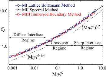
Figure 3: Data for the slip length $\xi$ from all three numerical methods for planar Couette flow clearly demonstrating both the diffuse- and sharp-interface limits for small and large $M\eta/l^{2}$ respectively. All the results here are in the slow flow regime, $Ca<0.01$, where the slip length is independent of the shear velocity.

Having shown our numerical results to capture both the sharp interface limit of $\xi\propto l_{D}$ for large $M\eta/l^{2}$, and the diffusive interface limit of $\xi\propto(l_{D}l)^{1/2}$ for small $M\eta/l^{2}$, we are now in a position to reprise carefully the scaling arguments put forward in the earlier literature for each of these two scaling forms separately, and to discuss the validity of the assumptions made in arriving at these functional forms.

We will follow a similar line of arguments as in Yue et al. (2010), where the Stokes and steady-state Cahn-Hilliard equations are integrated in the $x$-direction along the wall. For concreteness, let us focus on the contact line at the top wall, i.e. at $y=L_{y}$. The same scaling analysis applies for the bottom wall ($y=0$). For the $x$-component of the Stokes equation, this gives

$$\int_{-\infty}^{\infty}\left[\eta\frac{\partial^{2}v_{x}}{\partial y^{2}}+\eta\frac{\partial^{2}v_{x}}{\partial x^{2}}-\frac{\partial p}{\partial x}-\phi\frac{\partial\mu}{\partial x}\right]dx=0.$$ (19)

The second term can be integrated to $\eta\partial v_{x}/\partial x|_{-\infty}^{\infty}=0$. The contribution of the third term in the integral is also zero, because the pressure attains the same, constant value on either side of the interface, far from the contact line. The fourth (final) term scales as $\mu_{\rm{max}}$, which represents the magnitude of the chemical potential for a given flow setup.

The first term in Eq. 19 needs to be analysed more carefully. In the sharp interface limit, the term $\partial^{2}v_{x}/\partial y^{2}$ scales as $V_{0}/\xi^{2}$, and this term is significant across a length scale given by the slip length $\xi$. Thus, we have

$$\eta\frac{V_{0}}{\xi^{2}}\xi\sim\mu_{\rm{max}},$$

$$\mu_{\rm{max}}\sim\eta V_{0}/\xi.$$ (20)

In the diffuse interface limit, the fluid velocity still varies across a length scale $\xi$ in the $y$-direction, and as such, the term $\partial^{2}v_{x}/\partial y^{2}$ still scales as $V_{0}/\xi^{2}$. However, to capture the key physics, the spatial window of integration must be broadened to the interface width $l$, since here $\xi$ is less than the interfacial width $l$: recall the bottom leftmost data points in Fig. 3. Taking the suitable of window of integration into account, Eq. 19 leads to

$$\eta\frac{V_{0}}{\xi^{2}}l\sim\mu_{\rm{max}},$$

$$\mu_{\rm{max}}\sim\eta V_{0}l/\xi^{2}.$$ (21)

Let us now carry out a similar analysis for the Cahn-Hilliard equation,

$$\int_{-\infty}^{\infty}\left[v_{x}\frac{\partial\phi}{\partial x}+v_{y}\frac{\partial\phi}{\partial y}-M\frac{\partial^{2}\mu}{\partial x^{2}}-M\frac{\partial^{2}\mu}{\partial y^{2}}\right]dx=0.$$ (22)

The first term can be integrated to give $V_{0}\,\phi|_{-\infty}^{\infty}=2V_{0}$. The second term is zero simply because $v_{y}=0$ at $y=0$. The third term integrates to $-M\partial\mu/\partial x|_{-\infty}^{\infty}$, which is again zero because $\partial\mu/\partial x=0$ far from the interface.

The result for the fourth term depends on the slip length regimes. $\partial^{2}\mu/\partial y^{2}$ scales as $\mu_{\rm{max}}/\xi^{2}$. However, the window of integration is different in the sharp ($\xi$) and diffuse ($l$) interface limits. For the sharp interface limit, the Cahn-Hilliard equation leads to the scaling

$$V_{0}\sim M\mu_{\rm{max}}/\xi.$$ (23)

On the other hand, for the diffuse interface limit, we obtain

$$V_{0}\sim M\mu_{\rm{max}}l/\xi^{2}.$$ (24)

We are now in the position to derive the scaling law predictions for the slip length. Combining Eqs. (20) and (23) gives

$$\xi\sim(M\eta)^{1/2}=l_{D}$$ (25)

in the sharp interface regime. Similarly, combining Eqs. (21) and (24) for the diffuse interface regime results in

$$\xi\sim(M\eta l^{2})^{1/4}=(l_{D}l)^{1/2}.$$ (26)

As seen in Fig. 3, in between the sharp and diffuse interface regimes is a smooth crossover where the behaviour varies smoothly from one scaling law to another. We define the crossover point by fitting the power laws in the sharp and diffuse interface regimes separately, and finding where these two fits intersect each other. This occurs at $l_{D}/l=0.38$, in broad agreement with the sharp interface criterion $l_{D}/l>0.25$ proposed by Yue et al. (2010)

We note finally that the values of the slip length presented in Fig. 3 are independent of the wall velocity, and correspondingly of the Capillary number $\mbox{{Ca}}=\eta V_{0}/\sigma$, provided $\mbox{{Ca}}\lesssim 0.01$. (Data not shown.) We shall demonstrate this independence explicitly below for the case of planar Poiseuille flow (see Fig. 5).

IV.2 Influence of a curvature term

In this section we test the extent to which our results for the slip length do or do not depend on the microscopic details of the diffuse interface model. Intuitively we might expect the slip length to be independent of microscopics in the sharp interface regime, but dependent on microscopics in the diffuse interface regime. Our numerical results below provide evidence in favour of this intuition, to which we shall however also add a note of caution at the end of this section.

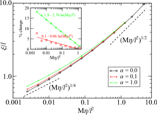
Figure 4: Numerical data demonstrating how slip lengths in the diffuse-interface limit are affected by the inclusion of a curvature free energy term. The results of the standard Landau theory ($\alpha=0$) are shown for comparison. Inset: percentage change relative to the case without curvature for $\alpha=0.1$ (red squares), $\alpha=1$ (green circles). These data are obtained using the spectral method (MII) in planar Couette flow.

There are many possible ways to modify the basic Landau theory for which we presented results in the previous subsection. We focus here on the simple but non-trivial extension made by introducing the additional interfacial curvature term with a strength set by $\alpha$ in Eq. (5). Fig. 4 shows our numerical results for $\alpha=0.1$ and $1.0$. Shown in the same plot for comparison are our original results, already presented in the previous subsection, for the original theory with $\alpha=0$. As can be seen, the introduction of the curvature term affects the slip length quite strongly in the diffuse interface regime. This is to be expected: in this regime the physics of the problem is determined not only by macroscopic quantities, but by the microscopic gradient contributions to the free energy. In contrast, as the control parameter $M\eta/l^{2}$ increases into the sharp interface regime the dependence of the slip length on this microscopic parameter $\alpha$ dramatically decreases and appears to become negligible in the sharp interface limit $M\eta/l^{2}\to\infty$.

Although these numerical results strongly suggest that the slip length is independent of the microscopic (gradient) contributions to the free energy in the sharp interface regime, we attach the following note of caution. In the case of equilibrium phase coexistence in the absence of flow, it is possible to show by integrating across the interface between the phases that macroscopic bulk quantities, such as the value of the chemical potential at phase coexistence, are independent of the structure of that interface, as determined by the spatial gradient terms in the free energy. However the same is not true in general for the case of phase coexistence under the non-equilibrium conditions of an applied flow because the equations of motion are usually non-integrable in that case: they cannot be integrated across the interface to give a result that depends only on the bulk quantities on either side of the interface, but the result instead retains a dependence on the structure of the interface itself. This issue has been discussed in particular detail in the case of stress selection in shear banded flows (Olmsted and David Lu, 1999; Lu et al., 2000). Therefore, while our numerical results do strongly suggest that the slip length is independent of the gradient terms in the sharp interface limit, this question merits some further attention in future studies.

IV.3 Relation to Cox’s result

The results presented so far have demonstrated that, in the sharp interface limit, the emergent slip length is determined by the macroscopic dynamical variables $\eta$ and $M$. While this is clearly an important finding in terms of our physical understanding of the moving contact line problem, in numerical practice this sharp interface limit $M\eta/l^{2}\rightarrow\infty$ can be difficult to attain. Indeed the time taken to attain a steady state after the inception of flow increases dramatically with increasing $M\eta/l^{2}$. Lengthy simulations were required to obtain the rightmost data points in Fig. 3, with the extreme cases requiring run times of the order of weeks with a parallelised code using 4 cores of Intel(R) Xeon(R) 2.40Ghz.

With this in mind, we now turn to address two questions of practical numerical importance: (i) whether simulations carried out in the diffuse interface regime still reproduce the expected macroscopic dynamics far from the contact line, and (ii) whether our definition of the slip length is still meaningful outside the sharp interface regime. We shall address these questions in the context of the Poiseuille flow protocol sketched in Fig. 1b, in particular asking whether the dependence of the observed dynamic contact angle on flow velocity is the same in the diffuse interface regime as in the sharp interface regime.

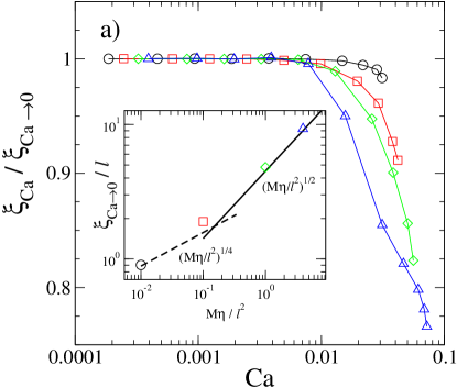
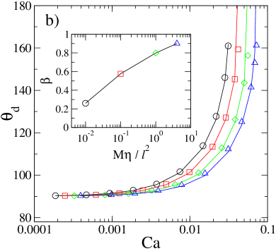
Figure 5: Numerical data for the Poiseuille flow protocol, for $M\eta/l^{2}=0.01$ (black circles $\bigcirc$), $0.1$ (red squares), $1$ (green diamonds), $4$ (blue triangles). a) Demonstration that the slip length converges to a constant value as $\mbox{{Ca}}\to 0$. The inset shows that the measured value of $\xi_{\mbox{{Ca}}\to 0}$ using the Poiseuille flow protocol is in good agreement with the best fit power laws obtained for shear flow in Fig 3. b) Symbols mark the dynamic contact angle $\theta_{d}$ as measured from simulation. The solid lines show the analytical predictions of Cox (1986) where $\delta=\beta\xi_{\mbox{{Ca}}}/L_{y}$. The inset shows the best fit values of $\beta$ which appear to converge $\beta\to 1$ in the sharp interface limit, $M\eta/l^{2}\to\infty$. The simulation data are obtained using the spectral method (MII).

We start by checking that the slip length obtained for the Poiseuille flow protocol is equivalent to that for planar Couette flow. Fig.  5a shows that the slip length for the Poiseuille case converges to a constant value as $\mbox{{Ca}}\to 0$, as for the planar Couette case. We have checked in this regime that the measured values of the slip length for the Couette and Poiseuille flows are within 0.5% of each other over the whole range of $M\eta/l^{2}$. See the inset of Fig. 5a, where the slip lengths for the Poiseuille flow are compared to the best fit power laws extracted for planar Couette flow in both the diffuse and sharp interface regimes. For larger $\mbox{{Ca}}>0.01$ the slip length starts to depend on the fluid velocity, as in planar Couette flow.

We now turn to the dynamic contact angle, as defined in Fig. 1b. It is known that this angle increases with increasing flow speed: for increasing pressure drop $\Delta P$ in Fig. 1b the interface is deformed more significantly due to the larger flow-speed mid channel compared to the stationary wall, and correspondingly the dynamic contact angle deviates more from the equilibrium value. Associated with this is a larger gradient in the chemical potential, which indeed allows the contact line to move at a higher velocity.

An analytical prediction for this increase of the dynamic contact angle with flow speed, as characterised by the capillary number Ca, was given by Cox (1986):

$$g(\theta_{d})=g(\theta_{e})+\mbox{{Ca}}\ln(\delta^{-1}).$$ (27)

Here $\theta_{d}$ is the dynamic contact angle and $\theta_{e}$ is the contact angle at equilibrium (here $90^{\circ}$). For fluids of matched viscosity the function $g$ is defined as

$$g(\theta)=\int_{0}^{\theta}\frac{\pi\phi(\pi-\phi)+(2\pi\phi-\pi^{2})\sin{\phi}\cos{\phi}-\pi\sin^{2}{\phi}}{2\pi^{2}\sin{\phi}}\,\,d\phi.$$ (28)

The parameter $\delta$ in Eqn. 27 is the ratio of the microscopic slip length to some characteristic macroscopic lengthscale of the system. We choose that to be the channel width $L_{y}$ and set $\delta=\beta\xi_{\mbox{{Ca}}}/L_{y}$ where $\beta$ is a constant fitting parameter.

To test Cox’s prediction, we plot our simulation results for the dependence $\theta_{d}$ on the capillary number Ca in Fig. 5b. We do so for four different values of $M\eta/l^{2}$, which we ensured span both the diffuse and sharp interface limits, as well as the crossover regime between them. Pleasingly we find excellent agreement with Cox’s prediction across the the full range of Ca, for all values of $M\eta/l^{2}$. Furthermore, as shown in the inset of Fig. 5b, the fitting parameter $\beta$ appears suggestively to converge to unity in the sharp interface limit, $M\eta/l^{2}\to\infty$.

These results suggest that simulations in the diffuse interface limit (and similarly the crossover regime) still provide a reliable representation of the macroscopic dynamics. However, the effective slip length must be suitably corrected by an $O(1)$ prefactor $\beta$. Increasingly minor corrections are needed as one approaches the sharp interface limit, and we expect Cox’s result would be directly obtained for $M\eta/l^{2}\to\infty$, where $\beta\to 1$.

V Conclusions

In this paper, we have performed extensive numerical simulations to reconcile previously apparently contradictory scaling laws for the slip length associated with a moving contact line in diffuse interface models. We did so by exploring four decades of the relevant dimensionless control parameter $M\eta/l^{2}=l_{D}^{2}/l^{2}$, and three decades of the capillary number $Ca$. Moreover we used three independent numerical methods, demonstrating their predictions to be in excellent quantitative agreement across all decades.

In the limit of slow flows corresponding to typical capillary numbers $Ca<0.01$, we find that the slip length converges to a well-defined value that is independent of the flow speed. In this slow flow regime we explored four decades in $M\eta/l^{2}=l_{D}^{2}/l^{2}$. Doing so enabled us to distinguish two distinct regimes for the scaling of the slip length, and a broad crossover window in between. For $M\eta/l^{2}\ll 1$ we found a diffuse interface regime in which the slip length scales as $\xi\sim(l_{D}l)^{1/2}$, consistent with the previous result of Briant and Yeomans (2004), and is furthermore sensitive to form of the microscopic interfacial terms in the free energy functional. In contrast for $M\eta/l^{2}\gg 1$ we recover the sharp interface limit previously discussed by Jacqmin (2000) and Yue et al. (2010). Here the slip length is proportional to the diffusion length scale, $\xi\propto l_{D}\sim(M\eta)^{1/2}$, depending only on the macroscopic dynamical variables of viscosity $\eta$ and molecular mobility $M$. Our numerical results further suggest the slip length to be insensitive to changes in the microscopic interfacial free energy terms in this sharp interface regime.

For $Ca>0.01$, the effective slip length decreases with increasing capillary number, in qualitative agreement with the work of Chen et al. (2000). However, we are not able to reproduce their prediction $\xi\propto V_{0}^{-1/2}$ of in this fast flowing regime. More broadly, so far we are unable to find any reliable scaling law that is valid across a broad range of Capillary number, and for both the sharp and diffuse interface regimes.

Our numerical results also allow us to appraise suitable sets of simulation parameters. By comparing our simulation results for the dynamic contact angle to the analytical prediction by Cox (1986), we find excellent agreement if we allow the slip length to be rescaled by a dimensionless prefactor $\beta=O(1)$, which pleasingly appears to converge to unity in the sharp interface limit. In numerical practice, however, the sharp interface limit can be very expensive to realise, partly because the time taken to attain a steady state increases dramatically with increasing $M\eta/l^{2}$, and partly because the slip length is O(10) larger than the interface width, with demanding implications on the overall size of the simulation box. In the diffuse interface limit, in contrast, the timescale and lengthscale requirements are less stringent, and simulations accordingly much less expensive to perform. Our fits to the Cox formula suggest that a reliable representation of the macroscopic physics is nonetheless attainable even in the diffuse regime, provided the lengths are suitable rescaled by this corrective prefactor $\beta=O(1)$.

There are several avenues for future work. Firstly, it would be interesting to investigate how the two scaling regimes for contact line slip in diffuse interface models affect more complex flow problems, such as the macroscopic dynamics of a liquid droplet (Servantie and Muller, 2008; Mognetti et al., 2010; Thampi et al., 2013) or the criterion for the liquid entrainment (wetting failure) (Eggers, 2004; Sbragaglia et al., 2008), and whether similar renormalization of the slip length is adequate to account for their differences, as for the Poiseuille flow considered here. In these cases, we need to implement non-neutral wetting boundary conditions. We expect the prefactors of the scaling laws to change with contact angles, but not the exponents themselves.

Secondly, given the crossover we have reported in this study, it would be insightful to revisit the liquid-gas system and understand the sharp interface limit of this model. In the binary model the slip mechanism is diffusion, and as such, the slip length depends on the mobility parameter, in addition to the fluid viscosity and the interface width. In the liquid gas system, the mechanism is evaporation-condensation instead, and we expect the slip length to depend on the density ratio between the liquid and gas phases.

Thirdly, we note that we have taken the zero temperature limit in this work and have not accounted for thermal fluctuations. It will be interesting to study if such fluctuations simply broaden the effective interface width, or they give rise to new phenomena. For example, enhanced spreading due to thermal fluctuations has been reported by Davidovitch et al. (2005) and Gross and Varnik (2014).

Finally, experimental systems consisting of colloid-polymer mixtures are known to phase separate into colloid-rich and colloid-poor domains, with an interface width that is of order 1 micron (Aarts et al., 2004; Setu et al., 2015), much larger than the typical value for molecular fluids. Such a system can potentially be exploited to realise the different contact line slip regimes discussed here experimentally.

Acknowledgements: The research leading to these results has received funding from the European Research Council under the European Union’s Seventh Framework Programme (FP7/2007-2013) / ERC grant agreement number 279365.

References

- Cox (1986) R. G. Cox, J. Fluid Mech., 1986, 168, 169.
- Parker and Lawrence (2001) A. R. Parker and C. R. Lawrence, Nature, 2001, 414, 33–34.
- Zheng et al. (2007) Y. Zheng, X. Gao and L. Jiang, Soft Matter, 2007, 3, 178–182.
- Hu et al. (2003) D. L. Hu, B. Chan and J. W. M. Bush, Nature, 2003, 424, 663–666.
- Morrow (1990) N. R. Morrow, Journal of Petroleum Technology, 1990, 42, 1476–1484.
- Tabeling (2010) P. Tabeling, Introduction to Microfluidics, Oxford University Press, 2010.
- Huh and Scriven (1971) C. Huh and L. E. Scriven, Journal of Colloid and Interface Science, 1971, 35, 85 – 101.
- de Gennes (1985) P. G. de Gennes, Rev. Mod. Phys., 1985, 57, 827–863.
- Zhou and Sheng (1990) M.-Y. Zhou and P. Sheng, Phys. Rev. Lett., 1990, 64, 882–885.
- Spelt (2005) P. D. Spelt, Journal of Computational Physics, 2005, 207, 389 – 404.
- Renardy et al. (2001) M. Renardy, Y. Renardy and J. Li, J. Comput. Phys., 2001, 171, 243–263.
- Anderson et al. (1998) D. M. Anderson, G. B. McFadden and A. A. Wheeler, Annual Review of Fluid Mechanics, 1998, 30, 139–165.
- Jacqmin (2000) D. Jacqmin, J. Fluid Mech., 2000, 402, 57–88.
- Seppecher (1996) P. Seppecher, International Journal of Engineering Science, 1996, 34, 977 – 992.
- Briant et al. (2004) A. J. Briant, A. J. Wagner and J. M. Yeomans, Phys. Rev. E, 2004, 69, 031602.
- Pooley et al. (2009) C. M. Pooley, H. Kusumaatmaja and J. M. Yeomans, Eur. Phys. J. Special Topics, 2009, 171, 63–71.
- Diotallevi et al. (2009) F. Diotallevi, L. Biferale, S. Chibbaro, G. Pontrelli, F. Toschi and S. Succi, The European Physical Journal Special Topics, 2009, 171, 237–243.
- Briant and Yeomans (2004) A. J. Briant and J. M. Yeomans, Phys. Rev. E, 2004, 69, 031603.
- Yue et al. (2010) P. Yue, C. Zhou and J. J. Feng, J. Fluid Mech., 2010, 645, 279.
- Chen et al. (2000) H.-Y. Chen, D. Jasnow and J. Viñals, Phys. Rev. Lett., 2000, 85, 1686–1689.
- Bray (1994) A. J. Bray, Advances in Physics, 1994, 43, 357–459.
- Cahn (1977) J. W. Cahn, The Journal of Chemical Physics, 1977, 66, 3667–3672.
- Pooley et al. (2008) C. M. Pooley, H. Kusumaatmaja and J. M. Yeomans, Phys. Rev. E, 2008, 78, 056709.
- Gompper and Zschocke (1991) G. Gompper and S. Zschocke, EPL (Europhysics Letters), 1991, 16, 731.
- Jacqmin (1999) D. Jacqmin, Journal of Computational Physics, 1999, 155, 96 – 127.
- Ladd and Verberg (2001) A. Ladd and R. Verberg, Journal of Statistical Physics, 2001, 104, 1191–1251.
- Pozrikidis (2011) C. Pozrikidis, Introduction to Theoretical and Computational Fluid Dynamics, Oxford University Press, 2011.
- Eyre (1998) D. J. Eyre, Unpubl. Artic., 1998, 1–15.
- Guillén-González and Tierra (2013) F. Guillén-González and G. Tierra, J. Comput. Phys., 2013, 234, 140–171.
- Press et al. (1992) W. H. Press, S. A. Teukolsky, W. T. Vetterling and F. B. P., Numerical Recipes in C, Cambridge University Press, 1992.
- Peskin (2002) C. S. Peskin, Acta Numer., 2002, 11, 479–517.
- Lai and Peskin (2000) M.-C. Lai and C. S. Peskin, J. Comput. Phys., 2000, 160, 705–719.
- Olmsted and David Lu (1999) P. D. Olmsted and C.-Y. David Lu, Faraday Discuss., 1999, 112, 183–194.
- Lu et al. (2000) C.-Y. D. Lu, P. D. Olmsted and R. C. Ball, Phys. Rev. Lett., 2000, 84, 642–645.
- Servantie and Muller (2008) J. Servantie and M. Muller, The Journal of Chemical Physics, 2008, 128, 014709.
- Mognetti et al. (2010) B. M. Mognetti, H. Kusumaatmaja and J. M. Yeomans, Faraday Discuss., 2010, 146, 153–165.
- Thampi et al. (2013) S. P. Thampi, R. Adhikari and R. Govindarajan, Langmuir, 2013, 29, 3339–3346.
- Eggers (2004) J. Eggers, Phys. Rev. Lett., 2004, 93, 094502.
- Sbragaglia et al. (2008) M. Sbragaglia, K. Sugiyama and L. Biferale, Journal of Fluid Mechanics, 2008, 614, 471–493.
- Davidovitch et al. (2005) B. Davidovitch, E. Moro and H. A. Stone, Phys. Rev. Lett., 2005, 95, 244505.
- Gross and Varnik (2014) M. Gross and F. Varnik, Int. J. Mod. Phys. C, 2014, 25, 1340019.
- Aarts et al. (2004) D. G. A. L. Aarts, R. P. A. Dullens, H. N. W. Lekkerkerker, D. Bonn and R. van Roij, The Journal of Chemical Physics, 2004, 120, 1973–1980.
- Setu et al. (2015) S. A. Setu, R. P. A. Dullens, A. Hernández-Machado, I. Pagonabarraga, D. G. A. L. Aarts and R. Ledesma-Aguilar, Nature Communications, 2015, 6, 7297.