Effective Capacity in Multiple Access Channels with Arbitrary Inputs

Abstract

In this paper, we consider a two-user multiple access fading channel under quality-of-service (QoS) constraints. We initially formulate the transmission rates for both transmitters, where the transmitters have arbitrarily distributed input signals. We assume that the receiver performs successive decoding with a certain order. Then, we establish the effective capacity region that provides the maximum allowable sustainable arrival rate region at the transmitters’ buffers under QoS guarantees. Assuming limited transmission power budgets at the transmitters, we attain the power allocation policies that maximize the effective capacity region. As for the decoding order at the receiver, we characterize the optimal decoding order regions in the plane of channel fading parameters for given power allocation policies. In order to accomplish the aforementioned objectives, we make use of the relationship between the minimum mean square error and the first derivative of the mutual information with respect to the power allocation policies. Through numerical results, we display the impact of input signal distributions on the effective capacity region performance of this two-user multiple access fading channel.

I Introduction

With the growth in wireless networks, recent years witnessed a large body of research on cooperative transmissions [1]. The researchers in some of these studies concentrated on multiple access transmission scenarios and investigated these scenarios from an information-theoretic perspective [2, 3, 4, 5, 6, 7]. For instance, the authors in [3] defined the ergodic capacity region for multiple access fading channels and derived the optimal resource allocation policies that maximize this region. Similarly, addressing the optimal power allocation policies that achieve any point on the capacity region boundary subject to a sum-power constraint, Gupta et al. studied Gaussian parallel (non-interacting) multiple access channels [4]. Moreover, taking the vector fading multiple access channels, the authors examined the dynamic resource allocation policies as an important means to increase the sum capacity in uplink synchronous code-division multiple-access systems [7].

It is very well known that the use of discrete and finite constellation diagrams is required for input signaling in many practical systems. Different than the above studies where the authors consider Gaussian input signaling, the authors in [8] researched two-user Gaussian multiple access channels with finite input constellations. Equivalently, the authors in [9] considered parallel Gaussian channels with arbitrary inputs as well. They investigated the optimal power allocation that maximizes the mutual information subject to an average power constraint by exploiting the relationship between the mutual information and the minimum mean-square error (MMSE), which was established in [10]. Furthermore, the authors in [11] explored the optimal power policies that minimize the outage probability over block-fading channels with arbitrary input distributions that were subject to both peak and average power constraints. Power allocation policies for a two-way relay channel with arbitrary inputs were studied in low and high signal-to-noise ratio regimes. In another line of research, the author studied the multiple access multiple-input multiple-output channels, and showed the relationship between the input-output mutual information and the MMSE [12].

In the meantime, since the current wireless systems require data transmission with strict constraints on delay performance, cross-layer design concerns have become of interest to many system designers. Therefore, quality-of-service (QoS) requirements regarding buffer overflow and delay have been addressed in wireless communications studies regarding the Data-Link and Physical layers. In that regard, effective capacity was established as a measure to indicate the maximum sustainable rate at a transmitter queue by a given service (channel) process [13]. Consequently, effective capacity has been investigated in several different transmission scenarios [14, 15, 16]. More recently, Ozcan et al. studied the effective capacity of point-to-point channels and derived the optimal power allocation policies to maximize the system throughput by employing arbitrary input distributions under average power constraints.

In this paper, we focus on a two-user multiple access transmission scenario in which transmitters apply arbitrarily distributed input signaling under average power constraints and QoS requirements that are imposed as buffer overflow and delay probabilities. Our analysis can be easily expanded to multiple access scenarios with more than two transmitters. Our main contributions can be sorted as follows: Defining the effective capacity region by employing the effective capacity of each transmitter, we provide the optimal power allocation policies under an average transmission power constraint. We make use of the relationship between the mutual information and the MMSE in obtaining the power allocation policies. Furthermore, we attain the optimal decoding order that is administered at the receiver regarding the interplay between the channel fading coefficients.

II System Description

Figure 1: Channel model. We consider a two-user multiple access channel in which two transmitters are communicating with a single receiver. Each transmitter has a data buffer, and the receiver performs successive interference cancellation with a certain order.

II-A Channel Model

We consider a multiple access channel scenario in which two transmitters send data to one common receiver as seen in Figure 1. We initially assume that the data arrive at both transmitters from a source (or sources), and they are stored in the transmitters’ data buffers before being conveyed into the wireless channel. Then, each transmitter divides the available data into data packets and performs the encoding, modulation and transmission of each packet in frames of $T$ seconds. If a packet is received and decoded correctly by the receiver, the receiver sends a positive acknowledgment (ACK) to the corresponding transmitter (i.e., the transmitter that sends the packet), and the transmitter removes the packet from its buffer. Otherwise, the receiver sends a negative ACK (NACK) to the corresponding transmitter, and the transmitter resends the same packet. Thus, we impose certain QoS requirements in each transmitter buffer in order to control the buffer violation probabilities.

During the transmission in the channel, the input-output relation at time instant $t$ is given as

$$y(t)=\sqrt{P_{1}(t)}h_{1}(t)x_{1}(t)+\sqrt{P_{2}(t)} h_{2}(t)x_{2}(t)+w(t),$$

for $t=1,2,\cdots$. Above, $x_{1}(t)$ and $x_{2}(t)$ are the channel inputs at the corresponding transmitters (i.e., Transmitter 1 and 2, respectively, in Fig. 1), and $y(t)$ is the channel output at the receiver. $P_{1}(t)$ and $P_{2}(t)$ are the instantaneous power allocation policies employed by Transmitter 1 and 2, respectively, with the following average power constraint:

$$\mathbb{E}\{P_{1}(t)\}+\mathbb{E}\{P_{2}(t)\}\leq\overline{P},$$ (1)

where $\overline{P}$ is finite. Moreover, $w(t)$ denotes the zero-mean, circularly symmetric, complex Gaussian random variable with a unit variance, i.e., ${E}\{|w|^{2}\}=1$. The noise samples $\{w(t)\}$ are independent and identically distributed. Meanwhile, $h_{1}(t)$ and $h_{2}(t)$ represent the fading coefficients between Transmitter 1 and the receiver, and Transmitter 2 and the receiver, respectively. The magnitude squares of the fading coefficients are denoted by $z_{1}(t)=|h_{1}(t)|^{2}$ and $z_{2}(t)=|h_{2}(t)|^{2}$ with finite averages, i.e., ${E}\{z_{1}\}<\infty$ and ${E}\{z_{2}\}<\infty$. We consider a block-fading channel, and assume that the fading coefficients stay constant for a frame duration of $T$ seconds and change independently from one frame to another. The channel coefficients, $h_{1}$ and $h_{2}$, are perfectly known to the receiver and both transmitters, and hence, each transmitter can adapt its transmission power policy accordingly. We finally note that the available transmission bandwidth is $B$ Hz. In the rest of the paper, we omit the time index $t$ unless otherwise needed for clarity.

II-B Achievable Rates

We can express the instantaneous achievable rate between the transmitters and the receiver by invoking the mutual information between the inputs at the transmitters, i.e., $x_{1}$, $x_{2}$, and the output at the receiver, i.e., $y$. Hence, given that the instantaneous channel fading values, $h_{1}$ and $h_{2}$, are available at the transmitters and the receiver, the instantaneous achievable rate can be given as [17]

$$\mathcal{I}(x_{1},x_{2};y)=\mathbb{E}\left\{\log_{2}\frac{f_{y|x_{1},x_{2}}(y|x_{1},x_{2})}{f_{y}(y)}\right\},$$ (2)

where $f_{y}(y)=\sum_{x_{1},x_{2}}p(x_{1},x_{2})f_{y|x_{1},x_{2}}(y|x_{1},x_{2})$ is the marginal probability density function (pdf) of the received signal $y$ and

$$f_{y|x_{1},x_{2}}(y|x_{1},x_{2})=\frac{1}{\pi}e^{-|y-\sqrt{\alpha_{1}\overline{P}}h_{1}x_{1}-\sqrt{\alpha_{2}\overline{P}}h_{2}x_{2}|^{2}}.$$

Above, we consider the normalized power allocation policies: $\alpha_{1}=\frac{P_{1}}{\overline{P}}$ and $\alpha_{2}=\frac{P_{2}}{\overline{P}}$.

We assume that the receiver performs successive interference cancellation with a certain order $(j,m)$ for $j,m\in\{1,2\}$ and $j\neq m$. The decoding order depends on the channel conditions, i.e., the magnitude squares of channel fading coefficients, $z_{1}$ and $z_{2}$. In particular, the receiver initially decodes $x_{j}$ while treating $x_{m}$ as noise, and then subtracts $x_{j}$ from the received signal $y$ and decodes $x_{m}$. Let $\mathcal{Z}$ be the region of the $(z_{1},z_{2})$-space where the decoding order is (2,1). Then, $\mathcal{Z}^{c}$, which is the complement of $\mathcal{Z}$, is the region where the decoding order is (1,2). Now, we can express the instantaneous transmission rates for each transmitter as follows:

$$r_{1}(z_{1},z_{2})=\begin{cases}\mathcal{I}(x_{1};y_{1}),&\mathcal{Z},\\ \mathcal{I}(x_{1};y),&\mathcal{Z}^{c},\end{cases}$$ (3)

and

$$r_{2}(z_{1},z_{2})=\begin{cases}\mathcal{I}(x_{2};y),&\mathcal{Z},\\ \mathcal{I}(x_{2};y_{2}),&\mathcal{Z}^{c},\end{cases}$$ (4)

where

$$y_{1}=\sqrt{\alpha_{1}\overline{P}}h_{1}x_{1}+w,$$ (5)

$$y_{2}=\sqrt{\alpha_{2}\overline{P}}h_{2}x_{2}+w.$$

The decoding regions can be determined in such a way to maximize the objective throughput. Furthermore, we have

$$\mathcal{I}(x_{j};y_{j})=\mathbb{E}\left\{\log_{2}\frac{f_{y_{j}|x_{j}}(y_{j}|x_{j})}{f_{y_{j}}(y_{j})}\right\},$$

where $f_{y_{j}}(y_{j})=\sum_{x_{j}}p(x_{j})f_{y_{j}|x_{j}}(y_{j}|x_{j})$ is the marginal pdf of $y_{j}$ and

$$f_{y_{j}|x_{j}}(y_{j}|x_{j})=\frac{1}{\pi}e^{-|y_{j}-\sqrt{\alpha_{j}\overline{P}}h_{j}x_{j}|^{2}}.$$

II-C Effective Capacity

Recall that the data packets are stored in the buffers of the transmitters until they are reliably decoded by the receiver. Thus, the delay and buffer overflow concerns are of interest for system designers. Therefore, we concentrate on the data arrival processes, i.e., $a_{1}$ and $a_{2}$ in Fig. 1, and we propose the effective capacity that provides us the maximum constant arrival rate that a given service (channel) process can support in order to guarantee a desired statistical QoS specified with the QoS exponent $\theta$ [13].

Now, let $Q$ be the stationary queue length, then we can define the decay rate of the tail distribution of the queue length $Q$ as

$$\theta=-\lim_{q\to\infty}\frac{\log\text{Pr}(Q\geq q)}{q}.$$

Therefore, for large $q_{max}$ we can approximate the buffer violation probability as $\text{Pr}(Q\geq q_{max})\approx e^{-\theta q_{max}}$. Based on this relation, we can see that large $\theta$ indicates stricter QoS constraints, while smaller $\theta$ implies looser constraints. For a discrete-time, stationary and ergodic stochastic service process $r(t)$, the effective capacity is given by

$$-\lim_{t\to\infty}\frac{1}{\theta t}\log_{e}\mathbb{E}\{e^{-\theta S(t)}\},$$

where $S(t)=\sum_{\tau=1}^{t}r(\tau)$. Hence, the effective capacity identifies the asymptotic decay rate of buffer occupancy, and it can be considered as the dual of the effective bandwidth [18].

In the aforementioned multiple access transmission scenario, each transmitter has its own buffer to store the data, and it has its own QoS requirements. Therefore, we denote the decay rate of Transmitter 1 and Transmitter 2 by $\theta_{1}$ and $\theta_{2}$, respectively. Noting that the transmission bandwidth is $B$ Hz, the block duration is $T$ seconds, and the channel fading coefficients change independently from one transmission frame to another, we can express the effective capacity of each transmitter, i.e., the maximum sustainable data arrival rate at Transmitter $j$, in bits/sec/Hz as

$$-\frac{1}{\theta_{j}TB}\log_{e}\mathbb{E}\left\{e^{-\theta_{j}TBr_{j}(z_{1},z_{2})}\right\}\quad j\in\{1,2\},$$ (6)

where the expectation is taken over the $(z_{1},z_{2})$-space. Now, invoking the definition given in [19], we express the effective capacity region of the given multiple access transmission scenario as follows:

$$\mathcal{C}_{E}(\Theta)= \bigcup_{r_{1},r_{2}}\Big{\{}{C(\Theta)}\geq{\bf 0}:$$

$${C_{j}(\theta_{j})\leq-\frac{1}{\theta_{j}TB}\log_{e}\mathbb{E}\left\{e^{-\theta_{j}TBr_{j}(z_{1},z_{2})}\right\}}\Big{\}},$$ (7)

where $\Theta=[\theta_{1},\theta_{2}]$, and ${C(\Theta)}=[C_{1}(\theta_{1}),C_{2}(\theta_{2})]$ is the vector of the effective capacity values.

III Performance Analysis

In this section, we focus on maximizing the effective capacity region defined in (II-C) under the QoS guarantees required at each transmitter and the average total power constraint defined in (1). Noting that the effective capacity region is convex [20], our objective turns out to be maximizing the boundary surface of the region, which can be characterized by the following optimization problem [3]:

$$\max_{\begin{subarray}{c}\mathcal{Z},\mathcal{Z}^{c}\\ \mathbb{E}\{P_{1}\}+\mathbb{E}\{P_{2}\}\leq\overline{P}\end{subarray}}\lambda_{1}{C}_{1}(\theta_{1})+\lambda_{2}{C}_{2}(\theta_{2}),$$ (8)

for $\lambda_{1},\lambda_{2}\in[0,1]$ such that $\lambda_{1}+\lambda_{2}=1$. In order to solve this optimization problem, we first obtain the power allocation policies in defined decoding regions $\mathcal{Z}$ and $\mathcal{Z}^{c}$, and then we provide the optimal decoding regions.

III-A Optimal Power Allocation

Here, we study the optimal power allocation policies that solve the optimization problem in (8) in given decoding regions $\mathcal{Z}$ and $\mathcal{Z}^{c}$. In the subsequent result, we provide the following proposition that gives us the optimal power allocation policies:

Proposition 1

The optimal normalized power allocation policies, $\alpha_{1}$ and $\alpha_{2}$, that solve the optimization problem in (8) are the solutions of the following equalities:

$$\frac{\lambda_{1}}{\psi_{1}}e^{-\theta_{1}TBr_{1}(z)}\frac{dr_{1}(z)}{d\alpha_{1}}+\frac{\lambda_{2}}{\psi_{2}}e^{-\theta_{2}TBr_{2}(z)}\frac{dr_{2}(z)}{d\alpha_{1}}=\varepsilon,$$ (9)

$$\frac{\lambda_{2}}{\psi_{2}}e^{-\theta_{2}TBr_{2}(z)}\frac{dr_{2}(z)}{d\alpha_{2}}=\varepsilon,$$ (10)

for $z=(z_{1},z_{2})\in\mathcal{Z}$, and

$$\frac{\lambda_{1}}{\psi_{1}}e^{-\theta_{1}TBr_{1}(z)}\frac{dr_{1}(z)}{d\alpha_{1}}=\varepsilon,$$ (11)

$$\frac{\lambda_{1}}{\psi_{1}}e^{-\theta_{1}TBr_{1}(z)}\frac{dr_{1}(z)}{d\alpha_{2}}+\frac{\lambda_{2}}{\psi_{2}}e^{-\theta_{2}TBr_{2}(z)}\frac{dr_{2}(z)}{d\alpha_{2}}=\varepsilon,$$ (12)

for $z\in\mathcal{Z}^{c}$. Above, $\psi_{1}=\mathbb{E}_{z}\big{\{}e^{-\theta_{1}TBr_{1}(z)}\big{\}}$, $\psi_{2}=\mathbb{E}_{z}\big{\{}e^{-\theta_{2}TBr_{2}(z)}\big{\}}$, and $\varepsilon$ is the Lagrange multiplier of the average power constraint in (1).

Proof: See Appendix -A. $\hfill{\square}$

Above, the derivatives of the transmission rates with respect to the corresponding normalized power allocation policies are given as

$$\frac{dr_{1}(z)}{d\alpha_{1}}=\begin{cases}\frac{d\mathcal{I}(x_{1};y_{1})}{d\alpha_{1}},&\mathcal{Z},\\ \frac{d\mathcal{I}(x_{1};y)}{d\alpha_{1}},&\mathcal{Z}^{c},\end{cases}$$

$$\frac{dr_{2}(z)}{d\alpha_{2}}=\begin{cases}\frac{d\mathcal{I}(x_{2};y)}{d\alpha_{2}},&\mathcal{Z},\\ \frac{d\mathcal{I}(x_{2};y_{2})}{d\alpha_{2}},&\mathcal{Z}^{c},\end{cases}$$

and

$$\frac{dr_{m}(z)}{d\alpha_{j}}=\frac{d\mathcal{I}(x_{j};y)}{d\alpha_{j}}-\frac{d\mathcal{I}(x_{j};y_{j})}{d\alpha_{j}}$$

for $m,j\in\{1,2\}$ and $m\neq j$.

In the following theorem, we provide the derivatives of the mutual information expressions with respect to the normalized power allocation policies:

Theorem 1

Let, $h_{1}$, $h_{2}$, and $\overline{P}$ be given. In the multiple access transmission scenario described in Section II, the first derivative of the mutual information between $x_{j}$ and $y$ with respect to the power allocation policy, $\alpha_{j}$, is given by

$$\frac{d\mathcal{I}(x_{j};y)}{d\alpha_{j}}=\overline{P}z_{j}\text{MMSE}(x_{j};y)$$

$$\hskip 25.6073pt+\overline{P}\sqrt{\frac{\alpha_{m}}{\alpha_{j}}}\text{Re}\left(h_{j}h_{m}^{*}\mathbb{E}\left\{x_{j}x_{m}^{*}-\hat{x}_{j}(y)\hat{x}_{m}^{*}(y)\right\}\right),$$ (13)

and similarly, the derivative of the mutual information between $x_{j}$ and $y_{j}$ with respect to $\alpha_{j}$ is given by

$$\frac{d\mathcal{I}(x_{j};y_{j})}{d\alpha_{j}}=\overline{P}z_{j}\text{MMSE}(x_{j};y_{j}),$$ (14)

for $j,m\in\{1,2\}$, $j\neq m$, and $(\cdot)^{*}$ is the complex conjugate operation. In (13), the MMSE expression is given as

$$\text{MMSE}(x_{j};y)=1-\frac{1}{\pi}\int\frac{\big{|}\sum_{x_{j}}x_{j}p(x_{j})f_{y|x_{j}}(y|x_{j})\big{|}^{2}}{f_{y}(y)}\mathrm{d}y,$$

and the MMSE estimates of the channel inputs are

$$\hat{x}_{j}(y)=\frac{\sum_{x}x_{j}p(x)f_{y|x}(y|x)}{f_{y}(y)}.$$

Similarly, the MMSE expression in (14) is obtained by

$$\text{MMSE}(x_{j};y_{j})=1-\frac{1}{\pi}\int\frac{\big{|}\sum_{x_{j}}x_{j}p(x_{j})f_{y_{j}|x_{j}}(y_{j}|x_{j})\big{|}^{2}}{f_{y_{j}}(y_{j})}\mathrm{d}y_{j},$$

where $y_{1}$ and $y_{2}$ are as given in (5).

Proof: See Appendix -B. $\hfill{\square}$

As seen in (9)-(12), closed-form solutions for $\alpha_{1}$ and $\alpha_{2}$ cannot be obtained easily which is mainly due to the cross-relation between $\alpha_{1}$ and $\alpha_{2}$. For instance, $\alpha_{1}$ is a function of $\alpha_{2}$ as observed in (9) for $z\in\mathcal{Z}$, whereas $\alpha_{2}$ is a function of $\alpha_{1}$ as seen in (12) for $z\in\mathcal{Z}^{c}$. Therefore, we need to employ numerical techniques which consist of iterative solutions.

In the following, we wrap up the above steps into an iterative solution with two algorithms that can be used to obtain the optimal power policies in given decoding regions. In Algorithm 1, we obtain the optimal normalized power allocation policies $\alpha_{1}$ and $\alpha_{2}$.

Algorithm 1

1:Given $\lambda_{1}$, $\lambda_{2}$, $\mathcal{Z}$ and $\mathcal{Z}^{c}$;

2:Initialize $\psi_{1}$, $\psi_{2}$;

3:while True do

4:     Initialize $\varepsilon$;

5:     Initialize $\alpha_{1}$;

6:     while True do

7:         if $z\in\mathcal{Z}$ then

8:              For given $\alpha_{1}$, compute the optimal $\alpha_{2}$ by solving (10) ;

9:              For computed $\alpha_{2}$, compute the optimal $\alpha_{1}^{\star}$ by solving (9) ;

10:         else

11:              For given $\alpha_{1}$, compute the optimal $\alpha_{2}$ by solving (12) ;

12:              For computed $\alpha_{2}$, compute the optimal $\alpha_{1}^{\star}$ by solving (11) ;

13:         end if

14:         if $|\alpha_{1}-\alpha_{1}^{\star}|\leq\epsilon$ for small $\epsilon>0$ then

15:              break;

16:         else

17:              Set $\alpha_{1}=\alpha_{1}^{\star}$;

18:         end if

19:     end while

20:     Check if the average power constraint in (1) is satisfied with quality;

21:     If not, update $\varepsilon$ and return to Step 5

22:     Compute $\psi_{1}^{\star}=\mathbb{E}_{z}\big{\{}e^{-\theta_{1}nr_{1}(z)}\big{\}}$ and $\psi_{2}^{\star}=\mathbb{E}_{z}\big{\{}e^{-\theta_{2}nr_{2}(z)}\big{\}}$

23:     if $|\psi_{1}-\psi_{1}^{\star}|\leq\epsilon$ and $|\psi_{2}-\psi_{2}^{\star}|\leq\epsilon$ then

24:         break;

25:     else

26:         Set $\psi_{1}=\psi_{1}^{\star}$ and $\psi_{2}=\psi_{2}^{\star}$;

27:     end if

28:end while

Given $\lambda_{j}$ and $\psi_{j}$ for $j\in\{1,2\}$, it is shown in [21] that both (10) and (11) has at most one solution. We can further show that (9) has at most one solution for $\alpha_{1}$ when $\alpha_{2}$ is given, and that (12) has at most one solution for $\alpha_{2}$ when $\alpha_{1}$ is given. Then, we can guarantee that Steps 8, 9, 11 and 12 in Algorithm 1 will converge to a single unique solution. It is also clear that (9) and (11) are monotonically decreasing functions of $\alpha_{1}$, and (10) and (12) are monotonically decreasing functions of $\alpha_{2}$. Hence, in region $\mathcal{Z}$, we first obtain $\alpha_{2}$ by solving (10), and then we find $\alpha_{1}$ by solving (9) after inserting $\alpha_{2}$ into (9). Similarly, in region $\mathcal{Z}^{c}$, we first obtain $\alpha_{1}$ by solving (11), and then we find $\alpha_{2}$ by solving (12) after inserting $\alpha_{1}$ into (12). We can employ bisection search methods to obtain $\alpha_{1}$ and $\alpha_{2}$. In the above approach, when either $\alpha_{1}$ or $\alpha_{2}$ becomes negative, we set it to zero.

III-B Optimal Decoding Order

Following the optimal power allocation policies, we identify the optimal decoding order regions. We initially note that when there are no QoS requirements, i.e., $\theta_{1}=\theta_{2}=0$, the effective capacity region is reduced to be the ergodic capacity region. The authors in [22] showed that the ergodic capacity region is maximized when the symbol of the transmitter with the strongest channel is decoded first. Principally, when $z_{j}>z_{m}$, the symbol of Transmitter $j$ is decoded first, and then the symbol of Transmitter $m$ is decoded. Furthermore, the authors in [19] considered a special case and set $\theta_{1}=\theta_{2}=\theta$ for $\theta>0$. Then, they derived the optimal decoding order that maximizes the effective capacity region. However, their result is based on the assumption of Gaussian input signaling. Nevertheless, obtaining the optimal decoding order regions is a difficult task when $\theta_{1}\neq\theta_{2}$ and arbitrary input distribution is employed. In the following, we provide the optimal decoding order regions given that the transmitters have the equal queue decay rates, i.e., $\theta_{1}=\theta_{2}$, and they employ arbitrary input distributions.

Theorem 2

Let $h_{1}$, $h_{2}$, and $\overline{P}$ be given. Define $z_{2}^{\star}$ for any given $z_{1}\geq 0$, such that the decoding order is (2,1) when $z_{2}>z_{2}^{\star}$, and it is (1,2) otherwise for the given $z_{1}$. In the multiple access transmission scenario described in Section II, with arbitrary input distributions and the normalized power allocation policies at the transmitters, the optimal $z_{2}^{\star}$ for any given $z_{1}$ value is the solution of the following equality:

$$\mathcal{I}(x;y|z_{1},z_{2}^{\star})=\mathcal{I}(x_{1};y_{1}|z_{1})+\mathcal{I}(x_{2};y_{2}|z_{2}^{\star}).$$

Proof: See Appendix -C. $\hfill{\square}$

Figure 2: Effective capacity region, $C_{1}(\theta_{1})$ vs. $C_{2}(\theta_{2})$, when BPSK input signaling is employed for different values of $\overline{P}$ and $K$.

IV Numerical Results

In this section, we present the numerical results. Throughout the paper, we set the available channel bandwidth to $B=100$ Hz and the transmission duration block to $T=1$ sec.. We further assume that $h_{1}$ and $h_{2}$ are independent of each other and set $\mathbb{E}\{|h_{1}|^{2}\}=\mathbb{E}\{|h_{2}|^{2}\}=1$. Unless indicated otherwise, we set the QoS exponents $\theta_{1}=\theta_{2}=0.01$. We define the signal-to-noise ratio with $\frac{\overline{P}}{{E}\{|w|^{2}\}}=\overline{P}$ where ${E}\{|w|^{2}\}=1$.

We initially consider binary phase shift keying (BPSK) at both transmitters, and we plot the effective capacity region in Fig. 2. We have the results for different values of the signal-to-noise ratio, $\overline{P}$, and $K$. Recall that when $K=0$, the channel fading has a Rayleigh distribution, i.e., there is not a strong line-of-sight propagation path between the transmitters and the receiver. On the other hand, when $K>0$, there is a line-of-sight path between the transmitters and the receiver, and the line-of-sight propagation path becomes dominant with increasing $K$. As expected, with increasing $K$, the effective capacity region broadens. Moreover, we observe the broadening of the effective capacity region with increasing $\overline{P}$ more clearly.

Setting $K=-6.88$ dB, we plot the effective capacity region for different $\overline{P}$ values and signal modulation methods such as BPSK, quadrature amplitude modulation (QAM) and Gaussian distributed signaling in Fig. 3. We can easily notice that Gaussian input signaling has the best performance for both $\overline{P}=-5$ dB and $\overline{P}=0$ dB, while BPSK has the lowest performance. However, the performance gap is reduced with decreasing $\overline{P}$. Furthermore, we investigate the effect of the QoS exponent, $\theta$, on the effective capacity region in Fig. 4. Here, we set $\overline{P}=5$ dB and $K=-6.88$ dB, and compare the effective capacity region for different modulation techniques. As clearly seen, increasing $\theta$ results in a decrease in the effective capacity region since the system is subject to stricter QoS constraints. We can further observe that the performance gaps among the modulation techniques are smaller with increasing $\theta$. We finally display the effective capacity region for transmitters having different modulation methods than each other in Fig. 5. We can clearly notice that the transmitter with an input signal of higher modulation order can sustain higher effective capacity.

Figure 3: Effective capacity region, $C_{1}(\theta_{1})$ vs. $C_{2}(\theta_{2})$, considering different input signaling for $K=-6.88$ dB and different values of $\overline{P}$.

V Conclusion

In this paper, we have investigated the optimal power allocation policies that maximize the effective capacity region of a two-user multiple access channel with arbitrarily distributed input signals. We have formulated the relationship between the MMSE and the first derivative of the mutual information with respect to the power allocation policies. We have provided an algorithm that determines the optimal normalized power allocation policies. We have established the optimal decision region boundaries for successive interference cancellation at the receiver for given power allocation policies. Through numerical techniques, we have shown that the line-of-sight propagation path can significantly improve the effective capacity performance. We have further justified that the Gaussian input signaling has better performance and that the performance gap increases in higher signal-to-noise ratio regime.

Figure 4: Effective capacity region, $C_{1}(\theta_{1})$ vs. $C_{2}(\theta_{2})$, considering different input signaling for $K=-6.88$ dB, $\overline{P}=5$ dB and different values of $\theta=\theta_{1}=\theta_{2}$.

-A Proof of Proposition 1

Let us rewrite (6) for Transmitter 1 as

$$C_{1}(\theta_{1})= \frac{-1}{\theta_{1}TB}\log_{e}\bigg{\{}\mathbb{E}_{\mathcal{Z}}\{e^{-\theta_{1}TB\mathcal{I}(x_{1};y_{1})}\}$$

$$+\mathbb{E}_{\mathcal{Z}^{c}}\{e^{-\theta_{1}TB\mathcal{I}(x_{1};y)}\}\bigg{\}}$$

$$= \frac{-1}{\theta_{1}TB}\log_{e}\psi_{1},$$ (15)

and for Transmitter 2 as

$$C_{2}(\theta_{2})= \frac{-1}{\theta_{2}TB}\log_{e}\bigg{\{}\mathbb{E}_{\mathcal{Z}}\{e^{-\theta_{2}TB\mathcal{I}(x_{2};y)}\}$$

$$+\mathbb{E}_{\mathcal{Z}^{c}}\{e^{-\theta_{2}TB\mathcal{I}(x_{2};y_{2})}\}\bigg{\}}$$

$$= \frac{-1}{\theta_{2}TB}\log_{e}\psi_{2}.$$ (16)

Since the objective function in (II-C) is convex and the constraint (1) is linear with respect to $\alpha_{1}$ and $\alpha_{2}$, we can use the Lagrangian method to solve the optimization problem (8). We can form the Lagrangian as

$$\mathcal{B}=\lambda_{1}C_{1}(\theta_{1})+\lambda_{2}C_{2}(\theta_{2})$$

$$\hskip 28.45274pt-\varepsilon\{\mathbb{E}_{z\in\mathcal{Z}}\{\alpha_{1}+\alpha_{2}\}+\mathbb{E}_{z\in\mathcal{Z}^{c}}\{\alpha_{1}+\alpha_{2}\}-1\},$$

where $\varepsilon$ is the Lagrangian multiplier. Now, taking the derivatives of $\mathcal{B}$ with respect to $\alpha_{1}$ and $\alpha_{2}$ and setting them to zero, we obtain (9) and (12), respectively, when $z\in\mathcal{Z}$, and (11) and (10), respectively, when $z\in\mathcal{Z}^{c}$.

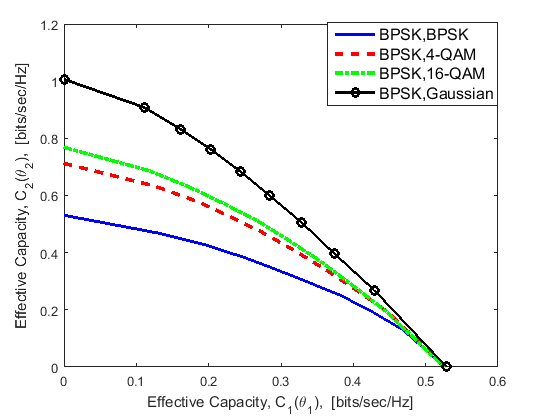
Figure 5: Effective capacity region, $C_{1}(\theta_{1})$ vs. $C_{2}(\theta_{2})$, considering mixed input signaling for $K=-6.88$ dB, $\overline{P}=0$ dB and $\theta_{1}=\theta_{2}=0.01$.

-B Proof of Theorem 1

Recall that $\alpha_{1}=\frac{P_{1}}{\overline{P}}$ and $\alpha_{2}=\frac{P_{2}}{\overline{P}}$, and

$$f(y)=\sum_{x}p(x)f(y|x),$$ (17)

where $x=(x_{1},x_{2})$. Since our analysis is performed in the complex plane, we can express $f(y|x)$ as

$$f(y|x)=\frac{1}{\pi}\text{exp} \bigg{\{}-\bigg{(}y_{r}-\sqrt{P_{1}}c_{1r}-\sqrt{P_{2}}c_{2r}\bigg{)}^{2}$$

$$-\bigg{(}y_{i}-\sqrt{P_{1}}c_{1i}-\sqrt{P_{2}}c_{2i}\bigg{)}^{2}\bigg{\}},$$ (18)

where $y=y_{r}+jy_{i}$, $h_{1}x_{1}=c_{1r}+jc_{1i}$ and $h_{2}x_{2}=c_{2r}+jc_{2i}$. The derivative of the pdf with respect to $P_{1}$ is given as

$$\frac{df(y|x)}{dP_{1}}=\frac{f(y|x)}{\sqrt{P_{1}}}\begin{pmatrix}c_{1r}&c_{1i}\end{pmatrix}\begin{pmatrix}y_{r}-\sqrt{P_{1}}c_{1r}-\sqrt{P_{2}}c_{2r}\\ y_{i}-\sqrt{P_{1}}c_{1i}-\sqrt{P_{2}}c_{2i}\end{pmatrix},$$

and

$$\frac{df(y|x)}{dy}=\dot{f}(y|x)=-2f(y|x)\begin{pmatrix}y_{r}-\sqrt{P_{1}}c_{1r}-\sqrt{P_{2}}c_{2r}\\ y_{i}-\sqrt{P_{1}}c_{1i}-\sqrt{P_{2}}c_{2i}\end{pmatrix}.$$ (19)

Hence, we have

$$\frac{df(y|x)}{dP_{1}}=\frac{-1}{2\sqrt{P_{1}}}\begin{pmatrix}c_{1r}&c_{1i}\end{pmatrix}\dot{f}(y|x).$$ (20)

Now, we can express

$$\frac{d\mathcal{I}(x_{1};y)}{dP_{1}}=\frac{d\mathcal{I}(x;y)}{dP_{1}}-\underbrace{\frac{d\mathcal{I}(x_{2};y_{2})}{dP_{1}}}_{=0}.$$ (21)

Invoking the marginal pdf $f(y|x)$ in (-B), we can rewrite the mutual information $\mathcal{I}(x;y)$ expressed in (2) as

$$\mathcal{I}(x;y)=-\log(\pi e)-\int f(y)\log(f(y))\mathrm{d}y.$$

Consequently, we can write (21) as

$$\frac{d\mathcal{I}(x_{1};y)}{dP_{1}}=\frac{d\mathcal{I}(x;y)}{dP_{1}}=-\frac{d}{dP_{1}}\int f(y)\log(f(y))\mathrm{d}y,$$

$$\hskip 48.36958pt=-\int[1+\log(f(y))]\frac{df(y)}{dP_{1}}\mathrm{d}y.$$ (22)

Substituting (17) and (20) in (22), we obtain

$$\frac{d\mathcal{I}(x_{1};y)}{dP_{1}}=$$

$$\frac{1}{2\sqrt{P_{1}}}\sum_{x}p(x)\begin{pmatrix}c_{1r}&c_{1i}\end{pmatrix}\int[1+\log(f(y))]\dot{f}(y|x)\mathrm{d}y.$$ (23)

Let $m=[1+\log(f(y))]$ and $dn=\dot{f}(y|x)\mathrm{d}y$, then the integration in (-B) can be evaluated using integration by part such that $\int mdn=mn\int ndm$. By noting that $mn=0$ as $y\to\infty$, we can write (-B) as

$$\frac{d\mathcal{I}(x_{1};y)}{dP_{1}}=\frac{-1}{2\sqrt{P_{1}}}\sum_{x}p(x)\begin{pmatrix}c_{1r}&c_{1i}\end{pmatrix}\int\frac{f(y|x)}{f(y)}\dot{f}(y|x)\mathrm{d}y.$$ (24)

By plugging (19) in (24), we have

$$\frac{d\mathcal{I}(x_{1};y)}{dP_{1}}$$

$$=\frac{1}{\sqrt{P_{1}}}\sum_{x}p(x)\begin{pmatrix}a_{1r}&a_{1i}\end{pmatrix}\int\frac{f(y|x)}{f(y)}\sum_{x}p(x)f(y|x)$$

$$\hskip 31.2982pt\times\begin{pmatrix}y_{r}-\sqrt{P_{1}}a_{1r}-\sqrt{P_{2}}a_{2r}\\ y_{i}-\sqrt{P_{1}}a_{1i}-\sqrt{P_{2}}a_{2i}\end{pmatrix}dy,$$

$$=\frac{1}{\sqrt{P_{1}}}\sum_{x}p(x)\begin{pmatrix}a_{1r}&a_{1i}\end{pmatrix}\int\frac{f(y|x)}{f(y)}\sum_{x}p(x)f(y|x)\begin{pmatrix}y_{r}\\ y_{i}\end{pmatrix}dy$$

$$\hskip 8.5359pt-\sum_{x}p(x)\begin{pmatrix}a_{1r}&a_{1i}\end{pmatrix}\int\frac{f(y|x)}{f(y)}\sum_{x}p(x)f(y|x)\begin{pmatrix}a_{1r}\\ a_{1i}\end{pmatrix}dy$$

$$\hskip 8.5359pt-\frac{\sqrt{P_{2}}}{\sqrt{P_{1}}}\sum_{x}p(x)\begin{pmatrix}a_{1r}&a_{1i}\end{pmatrix}$$

$$\hskip 88.2037pt\times\int\frac{f(y|x)}{f(y)}\sum_{x}p(x)f(y|x)\begin{pmatrix}a_{2r}\\ a_{2i}\end{pmatrix}dy,$$

$$=\frac{1}{\sqrt{P_{1}}}\sum_{x}p(x)\begin{pmatrix}a_{1r}&a_{1i}\end{pmatrix}\int f(y|x)\begin{pmatrix}y_{r}\\ y_{i}\end{pmatrix}dy$$

$$\hskip 8.5359pt-\int f(y)\begin{pmatrix}\widehat{a}_{1r}&\widehat{a}_{1i}\end{pmatrix}\begin{pmatrix}\widehat{a}_{1r}\\ \widehat{a}_{1i}\end{pmatrix}dy$$

$$\hskip 8.5359pt-\frac{\sqrt{P_{2}}}{\sqrt{P_{1}}}\int f(y)\begin{pmatrix}\widehat{a}_{1r}&\widehat{a}_{1i}\end{pmatrix}\begin{pmatrix}\widehat{a}_{2r}\\ \widehat{a}_{2i}\end{pmatrix}dy,$$

$$=\frac{1}{\sqrt{P_{1}}}\sum_{x}p(x)\begin{pmatrix}a_{1r}&a_{1i}\end{pmatrix}\begin{pmatrix}\sqrt{P_{1}}a_{1r}+\sqrt{P_{2}}a_{2r}\\ \sqrt{P_{1}}a_{1i}+\sqrt{P_{2}}a_{2i}\end{pmatrix}$$

$$\hskip 8.5359pt-\mathbb{E}\left\{\widehat{a}_{1r}^{2}+\widehat{a}_{1i}^{2}\right\}-\frac{\sqrt{P_{2}}}{\sqrt{P_{1}}}\mathbb{E}\left\{\widehat{a}_{1r}\widehat{a}_{2r}+\widehat{a}_{1i}\widehat{a}_{2i}\right\},$$

$$=\mathbb{E}\left\{a_{1r}^{2}+a_{1i}^{2}\right\}+\frac{\sqrt{P_{2}}}{\sqrt{P_{1}}}\mathbb{E}\left\{a_{1r}a_{2r}+a_{1i}a_{2i}\right\}$$

$$\hskip 8.5359pt-\mathbb{E}\left\{\widehat{a}_{1r}^{2}+\widehat{a}_{1i}^{2}\right\}-\frac{\sqrt{P_{2}}}{\sqrt{P_{1}}}\mathbb{E}\left\{\widehat{a}_{1r}\widehat{a}_{2r}+\widehat{a}_{1i}\widehat{a}_{2i}\right\},$$

$$=|h_{1}|^{2}\mathbb{E}\left\{|x_{1}|^{2}\right\}+\frac{\sqrt{P_{2}}}{\sqrt{P_{1}}}\text{Re}\left(h_{1}h_{2}^{\star}\mathbb{E}\left\{x_{1}x_{2}^{\star}\right\}\right)$$

$$\hskip 8.5359pt-|h_{1}|^{2}\mathbb{E}\left\{|\widehat{x}_{1}|^{2}\right\}-\frac{\sqrt{P_{2}}}{\sqrt{P_{1}}}\text{Re}\left(h_{1}h_{2}^{\star}\mathbb{E}\left\{\widehat{x}_{1}\widehat{x}_{2}^{\star}\right\}\right),$$

$$=|h_{1}|^{2}\text{MMSE}(x_{1};y)+\frac{\sqrt{P_{2}}}{\sqrt{P_{1}}}\text{Re}\left(h_{1}h_{2}^{\star}\mathbb{E}\left\{x_{1}x_{2}^{\star}-\widehat{x}_{1}\widehat{x}_{2}^{\star}\right\}\right).$$

Now, by applying the chain rule $\frac{d(\cdot)}{d\alpha_{1}}=\overline{P}\frac{d(\cdot)}{dP_{1}}$, we have

$$\frac{d\mathcal{I}(x_{1};y)}{d\alpha_{1}}=\overline{P}z_{1}\text{MMSE}(x_{1};y)$$

$$\hskip 65.44142pt+\overline{P}\sqrt{\frac{\alpha_{2}}{\alpha_{1}}}\text{Re}\left(h_{1}h_{2}^{\star}\mathbb{E}\left\{x_{1}x_{2}^{\star}-\widehat{x}_{1}\widehat{x}_{2}^{\star}\right\}\right).$$

Note that when the data of Transmitter 2 is subtracted from the received signal $y$, i.e, $\alpha_{2}=0$, the above equation is reduced to

$$\frac{d\mathcal{I}(x_{1};y_{1})}{d\alpha_{1}}=\overline{P}z_{1}\text{MMSE}(x_{1};y_{1}).$$

In a similar way, we can show that

$$\frac{d\mathcal{I}(x_{2};y)}{dP_{2}}=\overline{P}z_{2}\text{MMSE}(x_{2};y)$$

$$\hskip 65.44142pt+\overline{P}\sqrt{\frac{\alpha_{1}}{\alpha_{2}}}\text{Re}\left(h_{2}h_{1}^{\star}\mathbb{E}\left\{x_{2}x_{1}^{\star}-\widehat{x}_{2}\widehat{x}_{1}^{\star}\right\}\right).$$

and

$$\frac{d\mathcal{I}(x_{2};y_{2})}{d\alpha_{2}}=\overline{P}z_{2}\text{MMSE}(x_{2};y_{2}).$$

-C Proof of Theorem 2

We initially start by expressing the effective capacity of each user in (-A) and (-A) in the integration form and with respect to $z_{2}^{\star}$ and $\theta_{1}=\theta_{2}=\theta$ as

$$C_{1}(\theta,z_{2}^{\star})$$

$$=\frac{-1}{\theta n}\log_{e}\bigg{(}\int_{0}^{\infty}\int_{z_{2}^{\star}}^{\infty}e^{-\theta n\mathcal{I}(x_{1};y_{1}|z_{1})}p_{{z}}(z)\mathrm{d}z_{2}\mathrm{d}z_{1}$$

$$+\int_{0}^{\infty}\int_{0}^{z_{2}^{\star}}e^{-\theta n\mathcal{I}(x;y|z_{1},g(z_{1}))}e^{\theta n\mathcal{I}(x_{2};y_{2}|g(z_{1}))}p_{{z}}(z)\mathrm{d}z_{2}\mathrm{d}z_{1}\bigg{)},$$

and

$$C_{2}(\theta,z_{2}^{\star})$$

$$=\frac{-1}{\theta n}\log_{e}\bigg{(}\int_{0}^{\infty}\int_{0}^{z_{2}^{\star}}e^{-\theta n\mathcal{I}(x_{2};y_{2}|g(z_{1}))}p_{{z}}(z)\mathrm{d}z_{2}\mathrm{d}z_{1}$$

$$+\int_{0}^{\infty}\int_{z_{2}^{\star}}^{\infty}e^{-\theta n\mathcal{I}(x;y|z_{1},g(z_{1}))}e^{\theta n\mathcal{I}(x_{1};y_{1}|z_{1})}p_{{z}}(z)\mathrm{d}z_{2}\mathrm{d}z_{1}\bigg{)},$$

where $n=TB$. Let $\mathcal{B}(\hat{z_{2}})=\lambda_{1}C_{1}(\theta,\hat{z_{2}})+\lambda_{2}C_{2}(\theta,\hat{z_{2}})$, where $\hat{z_{2}}=z_{2}^{\star}+e\xi$, $z_{2}^{\star}$ is the optimal decoding function that solve the optimization problem (8), $e$ is a constant and $\xi$ represents an arbitrary deviation. Consequently, the following condition should be satisfied[25]:

$$\frac{d}{de}\mathcal{B}(\hat{z_{2}})\bigg{|}_{e=0}=0.$$ (25)

By noting that this condition holds for any $\xi$ and that $\frac{d\hat{z_{2}}}{de}=\xi$, solving (25) results in the following:

$$e^{-\theta n\mathcal{I}(x;y|z_{1},z_{2}^{\star})}\bigg{\{}\frac{-\lambda_{1}}{\psi_{1}}e^{\theta n\mathcal{I}(x_{2};y_{2}|z_{2}^{\star})}+\frac{\lambda_{2}}{\psi_{2}}e^{\theta n\mathcal{I}(x_{1};y_{1}|z_{1})}\bigg{\}}$$

$$=\frac{\lambda_{2}}{\psi_{2}}e^{-\theta n\mathcal{I}(x_{2};y_{2}|z_{2}^{\star})}-\frac{\lambda_{1}}{\psi_{1}}e^{-\theta n\mathcal{I}(x_{1};y_{1}|z_{1})}.$$ (26)

Now, let us denote $\mathcal{I}_{12}=\mathcal{I}(x;y|z_{1},z_{2}^{\star})$, $\mathcal{I}_{1}=\mathcal{I}(x_{1};y_{1}|z_{1})$ and $\mathcal{I}_{2}=\mathcal{I}(x_{2};y_{2}|z_{2}^{\star})$. Consequently, we can express (-C) as

$$e^{-\theta n\mathcal{I}_{12}}\bigg{\{}-\psi_{2}\lambda_{1}e^{\theta n\mathcal{I}_{2}}+\psi_{1}\lambda_{2}e^{\theta n\mathcal{I}_{1}}\bigg{\}}=$$ (27)

$$\hskip 96.73918pt-\psi_{2}\lambda_{1}e^{-\theta n\mathcal{I}_{1}}+\psi_{1}\lambda_{2}e^{-\theta n\mathcal{I}_{2}}.$$

Let us further define $A=e^{-\theta n\mathcal{I}_{2}}$ and $D=e^{-\theta n\mathcal{I}_{1}}$. Then, (27) can be rewritten as

$$e^{-\theta n\mathcal{I}_{12}}\bigg{\{}\frac{-\psi_{2}\lambda_{1}}{A}+\frac{\psi_{1}\lambda_{2}}{D}\bigg{\}}=-\psi_{2}\lambda_{1}D+\psi_{1}\lambda_{2}A,$$

which can be further simplified as

$$e^{-\theta n\mathcal{I}_{12}}=AD=e^{-\theta n\{\mathcal{I}_{1}+\mathcal{I}_{2}\}}.$$ (28)

Note that (28) implies that $\mathcal{I}_{12}=\mathcal{I}_{1}+\mathcal{I}_{2}$ which is equivalent to having

$$\mathcal{I}(x;y|z_{1},z_{2}^{\star})=\mathcal{I}(x_{1};y_{1}|z_{1})+\mathcal{I}(x_{2};y_{2}|z_{2}^{\star}).$$

References

- [1] X. Tao, X. Xu, and Q. Cui, “An overview of cooperative communications,” IEEE Commun. Mag., vol. 50, no. 6, pp. 65–71, 2012.
- [2] E. Biglieri and L. Györfi, Multiple Access Channels: Theory and Practice. IOS press, 2007.
- [3] D. N. C. Tse and S. V. Hanly, “Multiaccess fading channels. i. polymatroid structure, optimal resource allocation and throughput capacities,” IEEE Trans. Inf. Theory, vol. 44, no. 7, pp. 2796–2815, 1998.
- [4] G. A. Gupta and S. Toumpis, “Power allocation over parallel Gaussian multiple access and broadcast channels,” IEEE Trans. Inf. Theory, vol. 52, no. 7, pp. 3274–3282, 2006.
- [5] R. Knopp and P. A. Humblet, “Information capacity and power control in single-cell multiuser communications,” in IEEE Int. Commun. Conf. (ICC), vol. 1, 1995, pp. 331–335.
- [6] S. Vishwanath, S. Jafar, and A. Goldsmith, “Optimum power and rate allocation strategies for multiple access fading channels,” in IEEE Veh. Technol. Conf. Spring (VTC-SPRING), vol. 4, 2001, pp. 2888–2892.
- [7] P. Viswanath, D. N. C. Tse, and V. Anantharam, “Asymptotically optimal water-filling in vector multiple-access channels,” IEEE Trans. Inf. Theory, vol. 47, no. 1, pp. 241–267, 2001.
- [8] J. Harshan and B. S. Rajan, “On two-user Gaussian multiple access channels with finite input constellations,” IEEE Trans. Inf. Theory, vol. 57, no. 3, pp. 1299–1327, 2011.
- [9] A. Lozano, A. M. Tulino, and S. Verdú, “Optimum power allocation for parallel Gaussian channels with arbitrary input distributions,” IEEE Trans. Inf. Theory, vol. 52, no. 7, pp. 3033–3051, 2006.
- [10] D. Guo, S. Shamai, and S. Verdú, “Mutual information and minimum mean-square error in Gaussian channels,” IEEE Trans. Inf. Theory, vol. 51, no. 4, pp. 1261–1282, 2005.
- [11] K. D. Nguyen, A. Guillen i Fabregas, and L. K. Rasmussen, “Outage exponents of block-fading channels with power allocation,” IEEE Trans. Inf. Theory, vol. 56, no. 5, pp. 2373–2381, 2010.
- [12] S. A. Ghanem, “MAC gaussian channels with arbitrary inputs: Optimal precoding and power allocation,” in Int. Conf. Wireless Commun. Signal Process. (WCSP), 2012, pp. 1–6.
- [13] D. Wu and R. Negi, “Effective capacity: a wireless link model for support of quality of service,” IEEE Trans. Wireless Commun., vol. 2, no. 4, pp. 630–643, 2003.
- [14] J. Tang and X. Zhang, “Quality-of-service driven power and rate adaptation over wireless links,” IEEE Trans. Wireless Commun., vol. 6, no. 8, pp. 3058–3068, August 2007.
- [15] M. Gursoy, “MIMO wireless communications under statistical queueing constraints,” IEEE Trans. Inf. Theory, vol. 57, no. 9, pp. 5897–5917, Sept 2011.
- [16] S. Akin and M. Gursoy, “On the throughput and energy efficiency of cognitive MIMO transmissions,” IEEE Trans. Veh. Technol., vol. 62, no. 7, pp. 3245–3260, Sept 2013.
- [17] R. G. Gallager, Information theory and reliable communication. Springer, 1968, vol. 2.
- [18] C.-S. Chang, P. Heidelberger, S. Juneja, and P. Shahabuddin, “Effective bandwidth and fast simulation of ATM intree networks,” Elsevier Performance Evaluation, vol. 20, no. 1, pp. 45–65, 1994.
- [19] D. Qiao, M. C. Gursoy, and S. Velipasalar, “Achievable throughput regions of fading broadcast and interference channels under QoS constraints,” IEEE Trans. Commun., vol. 61, no. 9, pp. 3730–3740, 2013.
- [20] ——, “Transmission strategies in multiple-access fading channels with statistical QoS constraints,” IEEE Trans. Inf. Theory, vol. 58, no. 3, pp. 1578–1593, 2012.
- [21] G. Ozcan and M. C. Gursoy, “Qos-driven power control for fading channels with arbitrary input distributions,” in IEEE Int. Symp. Inform. Theory (ISIT), 2014, pp. 1381–1385.
- [22] N. Jindal, S. Vishwanath, and A. Goldsmith, “On the duality of Gaussian multiple-access and broadcast channels,” IEEE Trans. Inf. Theory, vol. 50, no. 5, pp. 768–783, 2004.
- [23] W. H. Jeong, J. S. Kim, M.-w. Jung, and K.-S. Kim, “MIMO channel measurement and analysis for 4G mobile communication,” in Springer Convergence Hybrid Inform. Technol., 2012, pp. 676–682.
- [24] D. Tse and P. Viswanath, Fundamentals of wireless communication. Cambridge university press, 2005.
- [25] G. B. Arfken, Mathematical methods for physicists. Academic press, 2013.