Concurrent learning for parameter estimation using dynamic state-derivative estimators

Abstract

A concurrent learning (CL)-based parameter estimator is developed to identify the unknown parameters in a linearly parameterized uncertain control-affine nonlinear system. Unlike state-of-the-art CL techniques that assume knowledge of the state-derivative or rely on numerical smoothing, CL is implemented using a dynamic state-derivative estimator. A novel purging algorithm is introduced to discard possibly erroneous data recorded during the transient phase for concurrent learning. Since purging results in a discontinuous parameter adaptation law, the closed-loop error system is modeled as a switched system. Asymptotic convergence of the error states to the origin is established under a persistent excitation condition, and the error states are shown to be ultimately bounded under a finite excitation condition. Simulation results are provided to demonstrate the effectiveness of the developed parameter estimator.

I Introduction

Modeling and identification of input-output relationships of nonlinear dynamical systems has been a long-standing active area of research. A variety of offline techniques have been developed for system identification; however, when models are used for online feedback control, the ability to adapt to changing environment and the ability to learn from input-output data are desirable. Motivated by applications in feedback control, online system identification techniques are investigated in results such as [1, 2, 3, 4] and the references therein.

Parametric methods such as linear parameterization, neural networks and fuzzy logic systems approximate the system identification problem by a finite-dimensional parameter estimation problem, and hence, are popular tools for online nonlinear system identification. Parametric models have been widely employed for adaptive control of nonlinear systems. In general, adaptive control methods do not require or guarantee convergence of the parameters to their true values. However, parameter convergence has been shown to improve robustness and transient performance of adaptive controllers (cf. [5, 6, 7, 8]). Parametric models have also been employed in optimal control techniques such as model-based predictive control (MPC) (cf. [9, 10, 11, 12]) and model-based reinforcement learning (MBRL) (cf. [13, 14, 15, 16]). In MPC and MBRL, the controller is developed based on the parameter estimates; hence, stability of the closed-loop system and the performance of the developed controller critically depend on convergence of the parameter estimates to their ideal values.

Data-driven concurrent learning (CL) techniques are developed in results such as [17, 8, 18], where recorded data is concurrently used with online data to achieve parameter convergence under a relaxed finite excitation condition as opposed to the persistent excitation (PE) condition required by traditional adaptive control methods. CL techniques employ the fact that a direct formulation of the parameter estimation error can be obtained provided the state-derivative is known or its estimate is otherwise available through techniques such as fixed-point smoothing [19]. The parameter estimation error can then be used in a gradient-based adaptation algorithm to drive the parameter estimates to their ideal values. If exact derivatives are not available, the parameter estimation error can be shown to decay to a neighborhood of the origin provided accurate estimates of the state-derivatives are available, where the size of the neighborhood depends on the derivative estimation error [19]. Experimental results such as [8] demonstrate that, since derivatives at past data points are required, noncausal numerical smoothing techniques can be used to generate satisfactory estimates of state-derivatives. Under Gaussian noise, smoothing is guaranteed to result in the best possible linear estimate corresponding to the available data [20, Section 5.3]; however, in general, the derivative estimation error resulting from numerical smoothing can not be quantified a priori. Furthermore, numerical smoothing requires additional processing and storage of data over a time-window that contains the point of interest. Hence, the problem of achieving parameter convergence under relaxed excitation conditions without using numerical differentiation is also motivated.

In this paper, an observer is employed to estimate the state-derivative. The derivative estimate generated by the observer converges exponentially to a neighborhood of the actual state-derivative. However, in the transient phase, the derivative estimation errors can be large. Since CL relies on repeated use recorded data, large transient errors present a challenge in the development of a CL-based parameter estimator. If the derivative estimation errors at the points recorded in the history stack are large, then the corresponding errors in the parameter estimates will be large. Motivated by the results in [21], the aforementioned challenge is addressed in this paper by designing a novel purging algorithm to purge possibly erroneous data from the history stack. The closed-loop error system along with the purging algorithm is modeled as a switched nonlinear dynamical system. Provided enough data can be recorded to populate the history stack after each purge, the developed method ensures asymptotic convergence of the error states to the origin.

The PE condition can be shown to be sufficient to ensure that enough data can be recorded to populate the history stack after each purge. Since PE can be an impractical requirement in many applications, this paper examines the behavior of the switched error system under a relaxed finite excitation condition. Specifically, provided the system states are exciting over a sufficiently long finite time-interval, the error states decay to an ultimate bound. Furthermore, the ultimate bound can be made arbitrarily small by increasing the learning gains. Simulation results are provided to demonstrate the effectiveness of the developed method under measurement noise.

II System dynamics

The system dynamics are assumed to be nonlinear, uncertain, and control-affine${}^{\ref{fn:CLNXDThe-focus-of}}$, described by the differential equation

$$\dot{x}=f\left(x,u\right),$$ (1)

where the function $f:\mathbb{R}^{n\times m}\to\mathbb{R}^{n}$ is locally Lipschitz. It is assumed that the dynamics can be split into a known component and an uncertain component with parametric uncertainties that are linear in the parameters. That is, $f\left(x,u\right)=f_{1}\left(x\right)+g\left(x\right)u+Y\left(x\right)\theta$, where $f_{1}:\mathbb{R}^{n}\to\mathbb{R}^{n}$, $g:\mathbb{R}^{n}\to\mathbb{R}^{n\times m}$ and $Y:\mathbb{R}^{n}\to\mathbb{R}^{n\times P}$ are known and locally Lipschitz continuous. The constant parameter vector $\theta\in\mathbb{R}^{P}$ is unknown, with a known bound $\overline{\theta}\in\mathbb{R}_{>0}$ such that $\left\|\theta\right\|<\overline{\theta}$. The objective is to design a parameter estimator to estimate the unknown parameters. The system input is assumed to be a stabilizing controller such that $x,\dot{x},u\in\mathcal{L}_{\infty}.$ The system state $x$ is assumed to be available for feedback, and the state-derivative $\dot{x}$ is assumed to be unknown.

III CL-based adaptive derivative estimation

Let $\hat{x}\in\mathbb{R}^{n}$ and $\dot{\hat{x}}\in\mathbb{R}^{n}$ denote estimates of the state $x$, and the state-derivative $\dot{x}$, respectively. Let $\hat{\theta}\in\mathbb{R}^{P}$ denote an estimate of the unknown vector $\theta$. To achieve convergence of the estimate $\hat{\theta}$ to the ideal parameter vector $\theta,$ a CL-based parameter estimator is designed. The motivation behind CL is to adjust the parameter estimates based on an estimate of the parameter estimation error $\tilde{\theta},$ defined as $\tilde{\theta}\triangleq\theta-\hat{\theta}$, in addition to the state estimation error $\tilde{x}.$ Since $\tilde{\theta}$ is not directly measurable, the subsequent development exploits the fact that the term $Y\left(x\right)\tilde{\theta}$ can be computed as $Y\left(x\right)\tilde{\theta}=\dot{x}-f_{1}\left(x\right)-g\left(x\right)u-Y\left(x\right)\hat{\theta}$, provided measurements of the state-derivative $\dot{x}$ are available. In CL results such as [17, 8, 18, 23], it is assumed that the state-derivatives can be computed with sufficient accuracy at a past time instance by numerically differentiating the recorded data. An approximation of the parameters estimation errors is then computed as $Y\left(x_{j}\right)\tilde{\theta}+\overline{d}=\dot{\overline{x}}_{j}-f_{1}\left(x_{j}\right)-g\left(x_{j}\right)u_{j}-Y\left(x_{j}\right)\hat{\theta}$, where $x_{j}$ denotes the system state at a past time instance $t_{j}$, $\dot{\overline{x}}_{j}$ denotes the numerically computed state-derivative at $t_{j}$, and $\overline{d}$ is a constant of the order of the error between $\dot{x}_{j}$ and $\dot{\overline{x}}_{j}$. While the results in [19] establish that, provided $\overline{d}$ is bounded, the parameter estimation error $\tilde{\theta}$ can be shown to decay to a ball around the origin, the focus is on the analysis of the effects of the differentiation error, and not on development of algorithms to reduce the parameter estimation error.

In this paper, a dynamically generated estimate of the state-derivative is used instead of numerical smoothing. The parameter estimation error is computed at a past recorded data point as $Y\left(x_{j}\right)\tilde{\theta}-\dot{\tilde{x}}_{j}=\dot{\hat{x}}_{j}-f_{1}\left(x_{j}\right)-g\left(x_{j}\right)u_{j}-Y\left(x_{j}\right)\hat{\theta}$, where $\dot{\tilde{x}}_{j}\triangleq\dot{x}_{j}-\dot{\hat{x}}_{j}$. To facilitate the design, let $\mathcal{H}\triangleq\left\{\left(\dot{\hat{x}}_{j},x_{j},u_{j}\right)\right\}_{j=1}^{M}$ be a history stack containing recorded values of the state, the control, and the state-derivative estimate. Each tuple $\left(\dot{\hat{x}}_{j},x_{j},u_{j}\right)$ is referred to as a data-point in $\mathcal{H}$. A history stack $\mathcal{H}$ is called “full rank” if the state vectors recorded in $\mathcal{H}$ satisfy $\mbox{rank}\left(\sum_{j=1}^{M}Y^{T}\left(x_{j}\right)Y\left(x_{j}\right)\right)=P$. Based on the subsequent Lyapunov-based stability analysis, the history stack is used to update the estimate $\hat{\theta}$ using the following update law:

$$\dot{\hat{\theta}}\!=\!k\Gamma\!\!\sum_{j=1}^{M}\!\!Y^{T}\!\left(\!x_{j}\!\right)\!\left(\!\dot{\hat{x}}_{j}\!-\!f_{1}\!\left(\!x_{j}\!\right)\!-\!g\!\left(\!x_{j}\!\right)\!u_{j}\!-\!Y\!\left(\!x_{j}\!\right)\!\hat{\theta}\!\right)\!+\!\Gamma Y^{T}\!\left(\!x\!\right)\!\tilde{x},$$ (2)

where $\tilde{x}=x-\hat{x}\in\mathbb{R}^{n}$, $\Gamma\in\mathbb{R}^{P\times P}$ and $k\in\mathbb{R}$ are positive and constant learning gains.

The update law in (2) drives the parameter estimation error to a ball around the origin, the size of which is of the order of $\dot{\tilde{x}}_{j}.$ Hence, to achieve a lower parameter estimation error, it is desirable to drive $\dot{\tilde{x}}$ to the origin. Based on the subsequent Lyapunov-based stability analysis, the following adaptive estimator is designed to generate the state-derivative estimates:

$$\dot{\hat{x}} =\gamma_{1}Y\left(x\right)\hat{\theta}+f_{1}\left(x\right)+g\left(x\right)u+\left(k_{1}+\alpha_{1}\right)\tilde{x}+\mu,$$

$$\dot{\mu} =\left(k_{1}\alpha_{1}+1\right)\tilde{x},$$ (3)

where $\mu\in\mathbb{R}^{n}$ is an auxiliary signal and $k_{1},\alpha_{1}\in\mathbb{R}_{>0}$ and $\gamma_{1}\in\left[0,1\right]$ are positive constant learning gains.

IV Algorithm to record the history stack

IV-A Purging of history stacks

The state-derivative estimator in (3) relies on feedback of the state estimation error $\tilde{x}.$ In general, feedback results in large transient estimation errors. Hence, the state-derivative estimation errors $\dot{\tilde{x}}_{j}$ associated with the tuples $\left(\dot{\hat{x}}_{j},x_{j},u_{j}\right)$ recorded in the transient phase can be large. The results in [19] imply that the parameter estimation errors can be of the order of $\max_{j}\left\|\dot{\tilde{x}}_{j}\right\|.$ Hence, if a history stack containing data-points with large derivative estimation errors is used for CL, then the parameter estimates will converge but the resulting parameter estimation errors can be large. To mitigate the aforementioned problem, this paper introduces a new algorithm that purges the erroneous data in the history stack as soon as more data is available. Since the estimator in (3) results in exponential convergence of $\dot{\hat{x}}$ to a neighborhood of $\dot{x},$ newer data is guaranteed to represent the system better than older data, resulting in a lower steady-state parameter estimation error. The following section details the proposed algorithm.

IV-B Algorithm to record the history stack

The history stack $\mathcal{H}$ is initialized arbitrarily to be full rank. An arbitrary full rank initialization of $\mathcal{H}$ results in a $\sigma-$modification (cf. [24]) like adaptive update law that keeps the parameter estimation errors bounded. However, since the history stack may contain erroneous data, the parameters may not converge to their ideal values.

In the following, a novel algorithm is developed to keep the history stack current by purging the existing (and possibly erroneous) data and replacing it with current data. The data collected from the system is recorded in an auxiliary history stack $\mathcal{G}\triangleq\left\{\left(\dot{\hat{x}}_{j}^{G},x_{j}^{G},u_{j}^{G}\right)\right\}_{j=1}^{M}$. The history stack $\mathcal{G}$ is initialized such that $\left(\dot{\hat{x}}_{j}^{G}\left(0\right),x_{j}^{G}\left(0\right),u_{j}^{G}\left(0\right)\right)=\left(\mathbf{0}_{n},\mathbf{0}_{n},\mathbf{0}_{m}\right)$ and is populated using a singular value maximization algorithm [17]. Once the history stack $\mathcal{G}$ becomes full rank with a minimum singular value that is above a (static or dynamic) threshold, $\mathcal{H}$ is replaced with $\mathcal{G}$, and $\mathcal{G}$ is purged. In this paper, a dynamic threshold is used which is set to be a fraction of the highest encountered minimum singular value corresponding to $\mathcal{H}$ up to the current time.

In the subsequent Algorithm 1, a piece-wise constant function $\delta:\mathbb{R}_{\geq 0}\to\mathbb{R}_{\geq 0}$, initialized to zero, stores the last time instance when $\mathcal{H}$ was updated and a piecewise constant function $\eta:\mathbb{R}_{\geq 0}\to\mathbb{R}_{\geq 0}$ stores the highest encountered value of $\sigma_{\mbox{min}}\left(\sum_{j=1}^{M}Y^{T}\left(x_{j}\right)Y\left(x_{j}\right)\right)$ up to time $t$, where $\sigma_{\mbox{min}}$ denotes the minimum singular value. The constant $\xi\in\left(0,1\right)$ denotes the threshold fraction used to purge the history stack, and $\mathcal{T}\in\mathbb{R}$ is an adjustable positive constant.

  if  a data point is available  then

     if  $\mathcal{G}$ is not full  then

         add the data to $\mathcal{G}$

     else

         add the data to $\mathcal{G}$ if $\sigma_{\mbox{min}}\left(\sum_{j=1}^{M}Y^{T}\left(x_{j}^{G}\right)Y\left(x_{j}^{G}\right)\right)$ increases

     end if

     if  $\sigma_{\mbox{min}}\left(\sum_{j=1}^{M}Y^{T}\left(x_{j}^{G}\right)Y\left(x_{j}^{G}\right)\right)\geq\xi\eta\left(t\right)$  then

        if  $t-\delta\left(t\right)\geq\mathcal{T}$  then

            $\mathcal{H}\leftarrow\mathcal{G}$ and $\mathcal{G}\leftarrow 0$ (purge $\mathcal{G}$)

            $\delta\left(t\right)\leftarrow t$

           if  $\eta\left(t\right)<\sigma_{\mbox{min}}\left(\sum_{j=1}^{M}Y^{T}\left(x_{j}\right)Y\left(x_{j}\right)\right)$  then

               $\eta\left(t\right)\leftarrow\sigma_{\mbox{min}}\left(\sum_{j=1}^{M}Y^{T}\left(x_{j}\right)Y\left(x_{j}\right)\right)$

           end if

        end if

     end if

  end if

Algorithm 1 History stack purging with dwell time

The following analysis establishes that if the system states are persistently exciting (in a sense that will be made clear in Theorem 1) then the parameter estimation error asymptotically decays to zero. Furthermore, it is also established that if the system states are exciting over a finite period of time, then the parameter estimation error can be made as small as desired provided $\mathcal{T}$ and the learning gains are selected based on the sufficient conditions introduced in Theorem 2.

V Analysis

V-A Asymptotic convergence with persistent excitation

Purging of the history stack $\mathcal{H}$ implies that the resulting closed-loop system is a switched system, where each subsystem corresponds to a history stack, and each purge indicates a switching event. To facilitate the analysis, let $\rho:\mathbb{R}_{\geq 0}\to\mathbb{N}$ denote a switching signal such that $\rho\left(0\right)=1$, and $\rho\left(t\right)=j+1$, where $j$ denotes the number of times the update $\mathcal{H}\leftarrow\mathcal{G}$ was carried out over the time interval $\left(0,t\right)$. In the following, the subscript $s\in\mathbb{N}$ denotes the switching index, and $\mathcal{H}_{s}$ denotes the history stack corresponding to the $s$^th subsystem (i.e., the history stack active during the time interval $\left\{t\mid\rho\left(t\right)=s\right\}$), containing the elements $\left\{\left(\dot{\hat{x}}_{sj},x_{sj},u_{sj}\right)\right\}_{j=1}^{M}$. To simplify the notation, let

$$A_{s}=\sum_{j=1}^{M}Y^{T}\left(x_{sj}\right)Y\left(x_{sj}\right),\>Q_{s}=\sum_{j=1}^{M}Y^{T}\left(x_{sj}\right)\dot{\tilde{x}}_{sj}.$$ (4)

Note that $A_{s}:\mathbb{R}_{\geq 0}\to\mathbb{R}^{P\times P}$ and $Q_{s}:\mathbb{R}_{\geq 0}\to\mathbb{R}^{P\times 1}$ are piece-wise constant functions of time. For ease of exposition, the constant $\mathcal{T}$ introduced in Algorithm 1 is set to zero for the case where persistent excitation is available.

Algorithm 1 ensures that there exists a constant $\underline{a}>0$ such that $\lambda_{\min}\left\{A_{s}\right\}\geq\underline{a},\>\forall s\in\mathbb{N},$ where $\lambda_{\mbox{min}}$ denotes the minimum eigenvalue. Since the state $x$ remains bounded by assumption, there exists a constant $\overline{A}$ such that $\left\|A_{s}\right\|\leq\overline{A},\>\forall s\in\mathbb{N}.$

Using (2) and (4), the dynamics of the parameter estimation error $\tilde{\theta}$ can be written as

$$\dot{\tilde{\theta}}=-\Gamma Y^{T}\left(x\right)\tilde{x}-k\Gamma A_{s}\tilde{\theta}+k\Gamma Q_{s}.$$ (5)

To establish convergence of the state-derivative estimates, a filtered tracking error $r\in\mathbb{R}^{n}$ is defined as $r\triangleq\dot{\tilde{x}}+\alpha_{1}\tilde{x}.$ Using (1), (3), and (5), the time derivative of the filtered tracking error can be expressed as,

$$\dot{r}=F\left(x,u\right)\tilde{\theta}-k\gamma_{1}Y\left(x\right)\Gamma A_{s}\tilde{\theta}-\gamma_{1}Y\left(x\right)\Gamma Y^{T}\left(x\right)\tilde{x}-\tilde{x}+k\gamma_{1}Y\left(x\right)\Gamma Q_{s}-k_{1}r,$$ (6)

where $F\left(x,u\right)\triangleq\gamma_{1}\nabla Y\left(x\right)Y\left(x\right)\theta+\gamma_{1}\nabla Y\left(x\right)f_{1}\left(x\right)+\gamma_{1}\nabla Y\left(x\right)g\left(x\right)u$ and $\nabla Y\left(x\right)\triangleq\partial Y\left(x\right)/x$.

To facilitate the stability analysis, let $\overline{F},$ $\overline{F}_{1},$ $\overline{x},$ $\overline{Y}$, and $\overline{\Gamma}$ be constants such that

$$\left\|F\left(x\left(t\right),u\left(t\right)\right)\right\|\leq\overline{F},\>\left\|Y\left(x\left(t\right)\right)\right\|\leq\overline{Y},\>\left\|\Gamma\right\|=\overline{\Gamma},$$

$$\left\|f_{1}\left(x\left(t\right)\right)+Y\left(x\left(t\right)\right)\theta+g\left(x\left(t\right)\right)u\left(t\right)\right\|\leq\overline{F}_{1},\>\left\|x\left(t\right)\right\|\leq\overline{x},$$ (7)

for all $t\in\mathbb{R}_{\geq 0}$. The following stability analysis is split into three parts. Under the temporary assumptions that the error states $\tilde{\theta}$, $\tilde{x}$, and $r$ are bounded at a switching instance and that the norms of the state-derivative estimates stored in the history stack are bounded, it is established in Part 1 that the error states $\tilde{\theta}$, $\tilde{x}$, and $r$ decay to a bound before the next switching instance, where the bound depends on the derivative estimation errors. Under the temporary assumption that the error states $\tilde{x}$ and $r$ are bounded at a switching instance, it is established in Part 2 that the derivative estimation error $\dot{\tilde{x}}$ can be made arbitrarily small before the next switching instance by increasing the learning gains. In Part 3, the temporary assumptions in Parts 1 and 2 are relaxed through an inductive argument where the results from Part 1 and Part 2 are used to conclude asymptotic convergence of the error states $\tilde{\theta},$ $\tilde{x}$, and $r$ to the origin.

Part 1: Boundedness of the error signals

Let $Z\triangleq\left[\begin{array}[]{ccc}r^{T}&\tilde{x}^{T}&\tilde{\theta}^{T}\end{array}\right]^{T}\in\mathbb{R}^{2n+L}$ and let $V:\mathbb{R}^{2n+P}\to\mathbb{R}_{\geq 0}$ denote a candidate Lyapunov function defined as

$$V\left(Z\right) \triangleq\frac{1}{2}r^{T}r+\frac{1}{2}\tilde{x}^{T}\tilde{x}+\frac{1}{2}\tilde{\theta}^{T}\Gamma^{-1}\tilde{\theta},$$ (8)

Using the Raleigh-Ritz Theorem, the Lyapunov function $V$ can be bounded as

$$\underline{v}\left\|Z\right\|^{2}\leq V\left(Z\right)\leq\overline{v}\left\|Z\right\|^{2},$$ (9)

where $\overline{v}\triangleq\frac{1}{2}\max\left\{1,\lambda_{\max}\left\{\Gamma^{-1}\right\}\right\},$ $\underline{v}\triangleq\frac{1}{2}\min\left\{1,\lambda_{\min}\left\{\Gamma^{-1}\right\}\right\}.$ The subsequent stability analysis assumes that the learning gains $k,$ $k_{1}$, and $\alpha_{1},$ and the matrices $A_{s}$ satisfy the following sufficient gain conditions:

$$\underline{a}>\frac{3\overline{Y}^{2}}{k\alpha_{1}}+\frac{4\overline{F}^{2}}{kk_{1}}+\frac{4k\overline{Y}^{2}\overline{\Gamma}^{2}\overline{A}^{2}}{k_{1}},\quad k_{1}>\frac{6\overline{Y}^{4}\overline{\Gamma}^{2}}{\alpha_{1}}.$$ (10)

The following Lemma establishes boundedness of the error state $Z$.

Lemma 1.

Let $T\in\mathbb{R}_{>0}$ be a constant such that $\rho\left(\tau\right)=s$, for all $\tau\in\left[t,t+T\right)$. Assume temporarily that there exist constants $\overline{H}_{s},\overline{V}_{s}\in\mathbb{R}_{>0}$ such that the elements of $\mathcal{H}_{s}$ satisfy $\left\|\dot{\hat{x}}_{j}\right\|\leq\overline{H}_{s}$, for all $j\in\left\{1,\cdots M\right\}$, and that the candidate Lyapunov function satisfies $V\left(Z\left(t\right)\right)\leq\overline{V}_{s}$. Then, the candidate Lyapunov function $V$ is bounded as

$$V\!\left(Z\!\left(\tau\right)\right)\!\leq\!\left(\!\overline{V}_{s}\!-\!\frac{\overline{v}}{v}\iota_{s}\!\right)\!e^{-\frac{v}{\overline{v}}\left(\tau-t\right)}\!+\!\frac{\overline{v}}{v}\iota_{s},\>\forall\tau\!\in\!\left[t,t+T\right),$$ (11)

where $\iota_{s}\triangleq\left(\frac{k}{2\underline{a}}+\frac{k^{2}\overline{Y}^{2}\overline{\Gamma}^{2}}{k_{1}}\right)\overline{Q}_{s}^{2}.$ Furthermore, the parameter estimation error can be bounded as

$$\left\|\tilde{\theta}\left(\tau\right)\right\|\leq\theta_{s},\>\forall\tau\in\left[t,t+T\right)$$ (12)

where $\theta_{s}\triangleq\sqrt{\frac{\>\overline{v}\>}{\underline{v}}}\max\left\{\sqrt{\overline{V}_{s}},\sqrt{\iota_{s}}\right\},$ $v\triangleq\min\left\{\frac{k\underline{c}}{4},\frac{\alpha_{1}}{3},\frac{k_{1}}{8}\right\},$ and $\overline{Q}_{s}\triangleq\left\|Q_{s}\right\|$.

Proof:

Using (5)-(6), the time derivative of the candidate Lyapunov function $V$ can be written as

$$\dot{V}=-\tilde{\theta}^{T}Y^{T}\left(x\right)\tilde{x}-k\tilde{\theta}^{T}A_{s}\tilde{\theta}+k\tilde{\theta}^{T}Q_{s}-\alpha_{1}\tilde{x}^{T}\tilde{x}+r^{T}F\left(x,u\right)\tilde{\theta}-k\gamma_{1}r^{T}Y\left(x\right)\Gamma A_{s}\tilde{\theta}-r^{T}\gamma_{1}Y\left(x\right)\Gamma Y^{T}\left(x\right)\tilde{x}\\ +k\gamma_{1}r^{T}Y\left(x\right)\Gamma Q_{s}-k_{1}r^{T}r.$$

Provided the sufficient conditions in (10) are satisfied, the Lyapunov derivative can be bounded as

$$\dot{V}\leq-\frac{k\underline{c}}{4}\left\|\tilde{\theta}\right\|^{2}-\frac{\alpha_{1}}{3}\left\|\tilde{x}\right\|^{2}-\frac{k_{1}}{8}\left\|r\right\|^{2}+\left(\frac{k}{2\underline{a}}+\frac{k^{2}\overline{Y}^{2}\overline{\Gamma}^{2}}{k_{1}}\right)\left\|Q_{s}\right\|^{2}.$$

Using the hypothesis that the elements of the history stack are bounded and the fact that $u$ is stabilizing, the Lyapunov derivative can be bounded as

$$\dot{V}\leq-\frac{v}{\overline{v}}V\left(Z\right)+\iota_{s}.$$

Using the comparison lemma [25, Lemma 3.4],

$$V\left(Z\left(\tau\right)\right)\leq\left(\!\overline{V}_{s}-\frac{\overline{v}}{v}\iota_{s}\!\right)e^{-\frac{v}{\overline{v}}\left(\tau-t\right)}+\frac{\overline{v}}{v}\iota_{s},\>\forall\tau\!\in\!\left[t,t+T\right).$$

If $\overline{V}_{s}\geq\frac{\overline{v}}{v}\iota_{s}$ then $V\left(Z\left(\tau\right)\right)\leq\overline{V}_{s}$. If $\overline{V}_{s}<\frac{\overline{v}}{v}\iota_{s}$ then $V\left(Z\left(\tau\right)\right)\leq\frac{\overline{v}}{v}\iota_{s}.$ Hence, using the definition of $Z$ and the bounds in (9), the bound in (12) is obtained. ∎

Part 2: Exponential decay of $\dot{\tilde{x}}$

Let $Z_{r}\triangleq\left[\begin{array}[]{cc}r^{T}&\tilde{x}^{T}\end{array}\right]^{T}\in\mathbb{R}^{2n}$ and let $V_{r}:\mathbb{R}^{2n}\to\mathbb{R}_{\geq 0}$ be a candidate Lyapunov function defined as $V_{r}\left(Z_{r}\right)\triangleq\left\|Z_{r}\right\|^{2}.$ The following lemma establishes exponential convergence of the derivative estimation error to a neighborhood of the origin using Lemma 1.

Lemma 2.

Let all the hypotheses of Lemma 1 be satisfied. Furthermore, assume temporarily that there exists a constant $\overline{V}_{rs}$ such that the candidate Lyapunov function $V_{r}$ satisfies $V_{r}\left(Z_{r}\left(t\right)\right)\leq\overline{V}_{rs}$. Then, the Lyapunov function $V_{r}$ is bounded as

$$V_{r}\!\left(\!Z_{r}\!\left(\tau\right)\!\right)\!\leq\!\left(\!\overline{V}_{rs}\!-\!\frac{\iota_{rs}}{v_{r}}\!\right)\!e^{-v_{r}\left(\tau-t\right)}\!+\!\frac{\iota_{rs}}{v_{r}},\>\forall\tau\!\in\!\left[t,t+T\right),$$ (13)

where $\nu_{r}=\min\left\{\frac{k_{1}}{2},\alpha_{1}\right\}$ and $\iota_{rs}\triangleq\frac{\left(\theta_{s}\overline{F}+k\overline{Y}\overline{\Gamma}\left(\theta_{s}\overline{A}+\overline{Q}_{s}\right)\right)^{2}}{k_{1}}.$ Furthermore, given a constant $\epsilon_{r}\in\mathbb{R}_{>0},$ the gain $k_{1}$ can be selected large enough such that $\left\|\dot{\tilde{x}}\left(t+T\right)\right\|\leq\epsilon_{r}$.

Proof:

Using (6), the time derivative of the candidate Lyapunov function $V_{r}$ can be written as

$$\dot{V}_{r}=-2r^{T}kY\left(x\right)\Gamma A_{s}\tilde{\theta}-2r^{T}Y\left(x\right)\Gamma Y^{T}\left(x\right)\tilde{x}+2r^{T}\left(\nabla Y\left(x\right)Y\left(x\right)\theta+\nabla Y\left(x\right)f_{1}\left(x\right)+\nabla Y\left(x\right)g\left(x\right)u\right)\tilde{\theta}\\ -2r^{T}\tilde{x}+k2r^{T}Y\left(x\right)\Gamma Q_{s}-k_{1}2r^{T}r+2\tilde{x}^{T}\left(r-\alpha_{1}\tilde{x}\right).$$

Completing the squares and using Lemma 1, the Lyapunov derivative can be bounded as

$$\dot{V}_{r}\leq-v_{r}V_{r}\left(Z_{r}\right)+\iota_{rs}.$$

Using the comparison lemma, [25, Lemma 3.4]

$$V_{r}\left(Z_{r}\left(\tau\right)\right)\leq\left(\!\overline{V}_{rs}-\frac{\iota_{rs}}{v_{r}}\!\right)\!e^{-v_{r}\left(\tau-t\right)}+\frac{\iota_{rs}}{v_{r}},\>\forall\tau\!\in\!\left[t,t+T\right).$$

Using the fact that, $\dot{\tilde{x}}=r-\alpha_{1}\tilde{x}$ the state-derivative estimation error can be bounded as

$$\left\|\dot{\tilde{x}}\right\|^{2}\leq\left\|r\right\|^{2}+\alpha_{1}\left\|\tilde{x}\right\|^{2}\leq\left(1+\alpha_{1}\right)V_{r}\left(Z_{r}\right).$$

Based on (13), given $\overline{V}_{rs}\geq V_{r}\left(Z_{r}\left(t\right)\right)$, $\epsilon_{r}>0$, the gain $k_{1}$ can be selected large enough so that $V_{r}\left(Z_{r}\left(t+T\right)\right)\leq\frac{\epsilon_{r}^{2}}{\left(1+\alpha_{1}\right)}$. Hence, given $\overline{V}_{rs},$ $\epsilon_{r}>0,$ the gain $k_{1}$ can be selected to be large enough so that $\left\|\dot{\tilde{x}}\left(t+T\right)\right\|\leq\epsilon_{r}.$ ∎

Part 3: Asymptotic convergence to the origin

Lemmas 1 and 2 employ the temporary hypothesis that the state-derivative estimates $\dot{\hat{x}}_{j}$ stored in the history stack remain bounded. However, since the estimates $\dot{\hat{x}}$ are generated dynamically using (3), they can not be guaranteed to be bounded a priori. In the following, the results of Lemmas 1 and 2 are used in an inductive argument to show that all the states of the dynamical system defined by (5)-(6) remain bounded and decay to the origin asymptotically provided enough data can be recorded to repopulate the history stack after each purge.

Theorem 1.

Provided the history stacks $\mathcal{H}$ and $\mathcal{G}$ are populated using Algorithm 1, the learning gains are selected to satisfy $\overline{V}_{r1}>\frac{\iota_{r1}}{v_{r}}$ and the sufficient gain conditions in (10), a bound $\overline{V}_{1}\in\mathbb{R}_{>0}$ is known such that $\overline{V}_{1}>\max\left(\frac{\overline{v}}{v}\iota_{1},V\left(Z\left(0\right)\right)\right)$, and provided the system states are exciting such that the history stack $\mathcal{H}$ can be persistently purged and replenished, i.e.,

$$s\to\infty,\>\mbox{as}\quad t\to\infty,$$ (14)

then, $\left\|\tilde{\theta}\left(t\right)\right\|\to 0$, $\left\|r\left(t\right)\right\|\to 0$, and $\left\|\tilde{x}\left(t\right)\right\|\to 0$ as $t\to\infty$.

Proof:

Let $\left\{T_{s}\in\mathbb{R}_{\geq 0}\mid s\in\mathbb{N}\right\}$ be a set of switching time instances defined as $T_{s}=\left\{t\mid\rho\left(\tau\right)<s+1,\>\forall\tau\in\left[0,t\right)\land\rho\left(\tau\right)\geq s+1,\>\forall\tau\in\left[t,\infty\right)\right\}.$ That is, for a given switching index $s,$ $T_{s}$ denotes the time instance when the $\left(s+1\right)$^th subsystem is switched on. To facilitate proof by mathematical induction, assume temporarily that the hypotheses of Lemmas 1 and 2 are satisfied for $t\in\left[0,T_{s}\right)$ for some $s$. Furthermore, assume temporarily that the following sufficient condition is satisfied:

$$\iota_{rj}>\iota_{r\left(j+1\right)},\quad\iota_{j}>\iota_{j+1},\quad\forall j\in\left\{1,2,\cdots,s-1\right\},$$ (15)

Then, using (11) and (13), the Lyapunov functions $V$ and $V_{r}$ can be bounded as $V\left(Z\left(t\right)\right)\leq W\left(t\right)\triangleq\left(\overline{V}_{1}-\frac{\overline{v}}{v}\iota_{1}\right)e^{-\frac{v}{\overline{v}}\left(t\right)}+\frac{\overline{v}}{v}\iota_{s}+\sum_{j=1}^{s-1}\frac{\overline{v}}{v}\left(\iota_{j}-\iota_{j+1}\right)e^{-\frac{v}{\overline{v}}\left(t-T_{j}\right)},$ and $V_{r}\left(Z_{r}\left(t\right)\right)\leq W_{r}\left(t\right)\triangleq\left(\overline{V}_{r1}-\frac{\iota_{r1}}{v_{r}}\right)e^{-v_{r}\left(t\right)}+\frac{\iota_{rs}}{v_{r}}+\sum_{j=1}^{s-1}\left(\frac{\iota_{rj}}{v_{r}}-\frac{\iota_{r\left(j+1\right)}}{v_{r}}\right)e^{-v_{r}\left(t-T_{j}\right)},$ where the constants $\iota_{s}$ and $\iota_{rs}$ were introduced in (11) and (13), respectively, and $W$, and $W_{r}$ denote the envelopes that bound the Lyapunov functions $V$ and $V_{r}$, respectively. Using the bounds on the Lyapunov functions, the bounding envelopes at consecutive switching instances can be related as

$$W\left(T_{s}\right)-W\left(T_{s-1}\right)=\frac{\overline{v}}{v}\left(\iota_{s-1}-\iota_{s}\right)\left(e^{\frac{v}{\overline{v}}\left(T_{s-1}-T_{s}\right)}-1\right)+\sum_{j=1}^{s-2}\frac{\overline{v}}{v}\left(\iota_{j}-\iota_{j+1}\right)e^{-\frac{v}{\overline{v}}\left(T_{s}-T_{j}\right)}\left(1-e^{\frac{v}{\overline{v}}\left(T_{s}-T_{s-1}\right)}\right)\\ +\left(\overline{V}_{1}-\frac{\overline{v}}{v}\iota_{1}\right)\left(e^{-\frac{v}{\overline{v}}\left(T_{s}\right)}-e^{-\frac{v}{\overline{v}}\left(T_{s-1}\right)}\right),$$

and

$$W_{r}\left(T_{s}\right)\!-\!W_{r}\left(T_{s-1}\right)\!=\!\left(\!\frac{\iota_{r\left(s-1\right)}}{v_{r}}-\frac{\iota_{rs}}{v_{r}}\!\right)\!\left(\!e^{v_{r}\left(T_{s-1}-T_{s}\right)}\!-\!1\!\right)+\sum_{j=1}^{s-2}\left(\frac{\iota_{rj}}{v_{r}}-\frac{\iota_{r\left(j+1\right)}}{v_{r}}\right)e^{-v_{r}\left(T_{s}-T_{j}\right)}\left(1-e^{v_{r}\left(T_{s}-T_{s-1}\right)}\right)\\ +\left(\overline{V}_{r1}-\frac{\iota_{r1}}{v_{r}}\right)\left(e^{-v_{r}\left(T_{s}\right)}-e^{-v_{r}\left(T_{s-1}\right)}\right).$$

Since $T_{s}>T_{s-1},$ the terms $\left(e^{-\frac{v}{\overline{v}}\left(T_{s}\right)}-e^{-\frac{v}{\overline{v}}\left(T_{s-1}\right)}\right)$, $\left(1-e^{v_{r}\left(T_{s}-T_{s-1}\right)}\right)$, $\left(1-e^{v_{r}\left(T_{s}-T_{s-1}\right)}\right),$ $\left(e^{\frac{v}{\overline{v}}\left(T_{s-1}-T_{s}\right)}-1\right)$, $\left(e^{-v_{r}\left(T_{s}\right)}-e^{-v_{r}\left(T_{s-1}\right)}\right)$, and $\left(e^{v_{r}\left(T_{s-1}-T_{s}\right)}-1\right)$ are always negative. By selecting $\overline{V}_{1}$ as

$$\overline{V}_{1}>\max\Biggl{(}\frac{\overline{v}}{v}\iota_{1},\overline{v}\biggl{(}\overline{F}_{1}^{2}+\overline{\theta}^{2}+\left\|\dot{\hat{x}}\left(0\right)\right\|^{2}+\left(1+\alpha_{1}\right)^{2}\left\|\tilde{x}\left(0\right)\right\|^{2}+\left\|\hat{\theta}\left(0\right)\right\|^{2}\biggr{)}\Biggr{)}$$ (16)

and using (15) and the hypotheses of Theorem 1, then $W\left(T_{s}\right)<W\left(T_{s-1}\right)$ and $W_{r}\left(T_{s}\right)<W_{r}\left(T_{s-1}\right)$.

Since the history stack $\mathcal{H}_{1}$ is selected at random to include bounded elements, all the hypotheses of Lemmas 1 and 2 are satisfied over the time interval $\left[0,T_{1}\right)$. Hence, $V\left(Z\left(t\right)\right)\leq W\left(t\right)=\left(\overline{V}_{1}-\frac{\overline{v}}{v}\iota_{1}\right)e^{-\frac{v}{\overline{v}}\left(t\right)}+\frac{\overline{v}}{v}\iota_{1}$, where $\iota_{1}=\left(\frac{k}{2\underline{a}}+\frac{k^{2}\overline{Y}^{2}\overline{\Gamma}^{2}}{k_{1}}\right)\overline{Q}_{1}^{2}$. Using the bounds in (7), $\overline{Q}_{1}$ can be computed as $\overline{Q}_{1}=qM\overline{Y}\left(\overline{F}_{1}+\overline{H}_{1}\right)$, where $q>1$ is an adjustable parameter. Furthermore, $V_{r}\left(Z_{r}\left(t\right)\right)\leq W_{r}\left(t\right)=\left(\overline{V}_{r1}-\frac{\iota_{r1}}{v_{r}}\right)e^{-v_{r}\left(t\right)}+\frac{\iota_{r1}}{v_{r}}$, where $\iota_{r1}=\frac{\left(\theta_{1}\overline{F}+k\overline{Y}\overline{\Gamma}\left(\theta_{1}\overline{A}+\overline{Q}_{1}\right)\right)^{2}}{k_{1}}$ and $\theta_{1}=\sqrt{\frac{\overline{v}}{\underline{v}}}\max\left\{\sqrt{\overline{V}_{1}},\sqrt{\iota_{1}}\right\}.$ Using the sufficient conditions $\overline{V}_{1}>\frac{\overline{v}}{v}\iota_{1}$ and $\overline{V}_{r1}>\frac{\iota_{r1}}{v_{r}}$ stated in Theorem 1, it can be concluded that $W\left(T_{1}\right)<W\left(0\right)$ and $W_{r}\left(T_{1}\right)<W_{r}\left(0\right)$. Selecting $\overline{V}_{2}=W\left(T_{1}\right)$ and $\overline{V}_{r2}=W_{r}\left(T_{1}\right)$, it can be concluded that $\overline{V}_{2}<\overline{V}_{1}$ and $\overline{V}_{r2}<\overline{V}_{r1}$.

Since the Lyapunov function $V_{r}$ does not grow beyond its initial condition over the time interval $\left[0,T_{1}\right)$, $\sup_{t\in\left[0,T_{1}\right)}\left\|\dot{\tilde{x}}\left(t\right)\right\|\leq\left(1+\alpha_{1}\right)\overline{V}_{r1}$. Moreover, since the history stack $\mathcal{H}_{2}$, which is active over the time interval $\left[T_{1},T_{2}\right)$, is recorded over the time interval $\left[0,T_{1}\right),$ all the hypotheses of Lemmas 1 and 2 are also satisfied over the time interval $\left[T_{1},T_{2}\right)$, and the constant $\overline{Q}_{2}$ can be computed as $\overline{Q}_{2}=M\overline{Y}\sqrt{2\left(1+\alpha_{1}\right)\overline{V}_{r1}}$. Provided $q$ is selected such that $q>\max\left\{1,\frac{\sqrt{2\left(1+\alpha_{1}\right)\overline{V}_{r1}}}{\left(\overline{F}_{1}+\overline{H}_{1}\right)}\right\},$ then $\overline{Q}_{2}<\overline{Q}_{1}.$ Hence, $\iota_{2}<\iota_{1}$. Since $\iota_{2}<\iota_{1}$ and $\overline{V}_{2}<\overline{V}_{1}$, then $\theta_{2}<\theta_{1},$ and hence, $\iota_{r2}<\iota_{r1}.$

Hence, by mathematical induction, the hypotheses of Lemmas 1 and 2 are satisfied for all $t\in\mathbb{R}_{\geq 0}$, and $V\left(Z\left(T_{s}\right)\right)<V\left(Z\left(T_{s-1}\right)\right)$ for all $s\in\mathbb{N}$. Hence, $V\left(Z\left(t\right)\right)\to 0$ as $t\to\infty.$ Since the Lyapunov function $V$ is common among all the subsystems, $Z\left(t\right)\to 0$ as $t\to\infty$ ∎

Theorem 1 implies that provided the system states are persistently excited such that the history stack $\mathcal{H}$ can always be replaced with a new full rank history stack, the state-derivative estimates, and the parameter estimate vector asymptotically converge to the state-derivative and the ideal parameter vector, respectively. However, from a practical perspective, it may be undesirable for a system to be in a persistently exciting state, or excitation beyond a certain finite time-interval may not be available. If excitation is available only over a finite time-interval, then the parameter estimation errors can be shown to be uniformly ultimately bounded, provided the history stacks are updated so that the time interval between two consecutive updates, i.e., the dwell time, is large enough. Algorithm 1 guarantees a minimum dwell time between two consecutive updates provided the constant $\mathcal{T}$ is selected large enough.

V-B Ultimate boundedness under finite excitation

For notational brevity, let $\beta_{1}\triangleq\left(\theta_{1}\overline{F}+k\overline{Y}\overline{\Gamma}\left(\theta_{1}\overline{A}+\overline{Q}_{1}\right)\right)^{2}$ and $\beta_{2}\triangleq\left(\frac{k}{2\underline{a}}+\frac{k^{2}\overline{Y}^{2}\overline{\Gamma}^{2}}{k_{1}}\right)$.

Theorem 2.

Let all the hypotheses of Theorem 1 be satisfied, except for the persistent excitation hypothesis in (14). Let $T\in\mathbb{R}_{>0}$ be a time instance such that $T_{s}<T$ for some $s>2$. Provided the history stacks are updated and populated using Algorithm 1, where the minimum dwell time satisfies

$$\mathcal{T}\geq\max_{j\in\left\{1,2,\cdots,s-1\right\}}\Biggl{\{}\frac{\overline{v}}{v\left(s-j\right)}\log\left(\frac{s\iota_{j}}{\iota_{s}}-\frac{s\iota_{j+1}}{\iota_{s}}\right),\frac{\overline{v}}{vs}\log\left(\frac{sv\overline{V}_{1}}{\overline{v}\iota_{s}}-\frac{s\iota_{1}}{\iota_{s}}\right),\frac{1}{v_{r}}\log\left(\frac{v_{r}\overline{V}_{r1}}{\iota_{r1}}-1\right)\Biggr{\}},$$

and the sufficient gain condition $k_{1}>\frac{8v_{r}\overline{v}^{2}M\overline{Y}\left(1+\alpha_{1}\right)\beta_{1}\beta_{2}^{2}}{\underline{v}^{2}v^{2}\epsilon^{2}}$ is satisfied for a given $\epsilon>0,$ then $\sup_{t>T}\left\|\tilde{\theta}\left(t\right)\right\|\leq\epsilon$.

Proof:

Since the history stack $\mathcal{H}_{1}$ is selected at random, all the hypotheses of Lemmas 1 and 2 are satisfied over the time interval $\left[0,T_{1}\right)$. Hence, $V\left(Z\left(t\right)\right)\leq W\left(t\right)=\left(\overline{V}_{1}-\frac{\overline{v}}{v}\iota_{1}\right)e^{-\frac{v}{\overline{v}}\left(t\right)}+\frac{\overline{v}}{v}\iota_{1}$, where $\iota_{1}=\beta_{2}\overline{Q}_{1}^{2}$. Using the bounds in (7), $\overline{Q}_{1}$ can be computed as $\overline{Q}_{1}=qM\overline{Y}\left(\overline{F}_{1}+\overline{H}_{1}\right)$, where $q>1$ is an adjustable parameter. Furthermore, $V_{r}\left(Z\left(t\right)\right)\leq W_{r}\left(t\right)=\left(\overline{V}_{r1}-\frac{\iota_{r1}}{v_{r}}\right)e^{-v_{r}\left(t\right)}+\frac{\iota_{r1}}{v_{r}}$, where $\iota_{r1}=\frac{\beta_{1}}{k_{1}}$ and $\theta_{1}=\sqrt{\frac{\overline{v}}{\underline{v}}}\max\left\{\sqrt{\overline{V}_{1}},\sqrt{\iota_{1}}\right\}.$ Provided $T_{1}>\frac{1}{v_{r}}\log\left(\frac{v_{r}\overline{V}_{r1}}{\iota_{r1}}-1\right)$, then $W_{r}\left(T_{1}\right)\leq\frac{2\iota_{r1}}{v_{r}}.$

Let $\epsilon_{1}>0$ be a constant, to be selected later. Provided the gain $k_{1}$ is selected such that $k_{1}>\frac{2v_{r}\left(1+\alpha_{1}\right)\beta_{1}}{\epsilon_{1}^{2}}$, then $\overline{V}_{r2}\leq\frac{\epsilon_{1}^{2}}{\left(1+\alpha_{1}\right)}$. Since $T_{2}<T$ by hypothesis, the Lyapunov envelope $W_{r}$ decays over the time interval $\left[T_{1},T_{2}\right)$; hence, $\sup_{t\in\left[T_{1},T_{2}\right)}\left\|\dot{\tilde{x}}\left(t\right)\right\|\leq\epsilon_{1}$, which implies $\overline{Q}_{3}$ can be selected as $\overline{Q}_{3}=M\overline{Y}\epsilon_{1}$ and $\iota_{3}=\beta_{2}M\overline{Y}\epsilon_{1}.$ Selecting $\epsilon_{1}=\frac{\underline{v}v\epsilon}{2\overline{v}\beta_{2}M\overline{Y}},$ the inequality $\iota_{3}\leq\frac{v\underline{v}\epsilon}{2\overline{v}}$ is obtained.

If the history stack $\mathcal{H}$ is not updated after the time instance $T_{s}$, then using an inductive argument similar to the proof of Theorem 1, it can be concluded that all the hypotheses of Lemma 1 are satisfied for all $t\in\left[T_{s},\infty\right)$. Hence, the Lyapunov function $V$ is bounded for all $t\in\left[T_{s},\infty\right)$ by

$$V\left(Z\left(t\right)\right)\leq\left(\overline{V}_{1}-\frac{\overline{v}}{v}\iota_{1}\right)e^{-\frac{v}{\overline{v}}\left(T_{s}\right)}+\frac{\overline{v}}{v}\iota_{s}+\sum_{j=1}^{s-1}\frac{\overline{v}}{v}\left(\iota_{j}-\iota_{j+1}\right)e^{-\frac{v}{\overline{v}}\left(T_{s}-T_{j}\right)}.$$

Since Algorithm 1 is designed to allow a minimum dwell time of $\mathcal{T}$ seconds, $T_{s}\geq s\mathcal{T}$ and $T_{s}-T_{j}\geq\left(s-j\right)\mathcal{T}$. Hence,

$$V\left(Z\left(T_{s}\right)\right)\leq\left(\overline{V}_{1}-\frac{\overline{v}}{v}\iota_{1}\right)e^{-\frac{v}{\overline{v}}\left(s\mathcal{T}\right)}+\frac{\overline{v}}{v}\iota_{s}+\sum_{j=1}^{s-1}\frac{\overline{v}}{v}\left(\iota_{j}-\iota_{j+1}\right)e^{-\frac{v}{\overline{v}}\mathcal{T}\left(s-j\right)}.$$

Provided the dwell time satisfies $\frac{\overline{v}}{vs}\log\left(\frac{sv\overline{V}_{1}}{\overline{v}\iota_{s}}-\frac{s\iota_{1}}{\iota_{s}}\right)\leq\mathcal{T},$ and $\frac{\overline{v}}{v\left(s-j\right)}\log\left(\frac{s\iota_{j}}{\iota_{s}}-\frac{s\iota_{j+1}}{\iota_{s}}\right)\leq\mathcal{T},\>\forall j\in\left\{1,2,\cdots,s-1\right\},$ then $V\left(Z\left(t\right)\right)\leq\frac{2\overline{v}\iota_{s}}{v}\leq\frac{2\overline{v}\iota_{3}}{v}$, for all $t\in\left[T_{s},\infty\right)$. Hence, using the bounds on the Lyapunov function in (9), $\left\|\tilde{\theta}\left(t\right)\right\|\leq\frac{2\overline{v}\iota_{3}}{\underline{v}v}$ for all $t\in\left[T_{s},\infty\right)$. Using the bound $\iota_{3}\leq\frac{v\underline{v}\epsilon}{2\overline{v}}$, $\left\|\tilde{\theta}\left(t\right)\right\|\leq\epsilon$ for all $t\in\left[T_{s},\infty\right)$. ∎

VI Simulation results

The developed technique is simulated using a model for a two-link robot manipulator arm. The four-dimensional state of the model is denoted by $x\triangleq\begin{bmatrix}x_{1}&x_{2}&x_{3}&x_{4}\end{bmatrix}^{T}$. The dynamics of the model are described by (1), where

$$f_{1}\left(x\right)=\begin{bmatrix}x_{3}\\ x_{4}\\ -\left(M\left(x\right)\right)^{-1}V_{m}\begin{bmatrix}x_{3}\\ x_{4}\end{bmatrix}\end{bmatrix},G\left(x\right)=\begin{bmatrix}\begin{array}[]{cc}0&0\end{array}\\ \begin{array}[]{cc}0&0\end{array}\\ \left(M\left(x\right)\right)^{-1}\end{bmatrix},Y\left(x\right)=\begin{bmatrix}\begin{array}[]{cccc}0&0&0&0\end{array}\\ \begin{array}[]{cccc}0&0&0&0\end{array}\\ \left[\begin{array}[]{cc}\left(M\left(x\right)\right)^{-1}&\left(M\left(x\right)\right)^{-1}\end{array}\right]D\left(x\right)\end{bmatrix}.$$ (17)

In (17), $D\left(x\right)\triangleq\mbox{diag}\left[x_{3},\>x_{4},\>\tanh\left(x_{3}\right),\>\tanh\left(x_{4}\right)\right]$, $M\left(x\right)\triangleq\begin{bmatrix}p_{1}+2p_{3}c_{2}\left(x\right),&p_{2}+p_{3}c_{2}\left(x\right)\\ p_{2}+p_{3}c_{2}\left(x\right),&p_{2}\end{bmatrix},$ and $V_{m}\left(x\right)\triangleq\begin{bmatrix}-p_{3}s_{2}\left(x\right)x_{4},&-p_{3}s_{2}\left(x\right)\left(x_{3}+x_{4}\right)\\ p_{3}s_{2}\left(x\right)x_{3},&0\end{bmatrix},$ where $c_{2}\left(x\right)=cos\left(x_{2}\right),$ $s_{2}\left(x\right)=sin\left(x_{2}\right)$, and $p_{1}=3.473$, $p_{2}=0.196$, and $p_{3}=0.242$ are constants. The system has four unknown parameters. The ideal values of the unknown parameters are $\theta=\begin{bmatrix}5.3&1.1&8.45&2.35\end{bmatrix}^{T}.$

The developed technique is compared against numerical differentiation-based concurrent learning where the numerical derivatives are computed using polynomial regression over a window of collected data. The state measurements are filtered using a moving average filter for state-derivative estimation. To facilitate the comparison, multiple simulation runs are performed using a combination of gains, window sizes, and thresholds for two levels of noise. The low-noise and high-noise simulations are performed by adding white Gaussian noise with variance 0.005 and 0.1, respectively, to the state measurements. The simulations are repeated five times for each combination of gains, and the gains, window sizes, and thresholds that yield the lowest steady-state RMS error over five runs are selected for comparison. Table I indicates that the developed technique outperforms numerical differentiation-based concurrent learning for both low-noise and high-noise cases. The following figures illustrate the performance of the developed technique in one sample run.

	Numerical differentiation-based CL		Developed technique
Noise variance	$0.005$	$0.1$	$0.005$	$0.1$
RMS steady-state error	$1.75$	$17.55$	$0.27$	$0.46$

Table I: Simulation results for the developed technique and numerical differentiation-based CL.

Figure 1a shows the evolution of the system state, where the added noise signal can be observed. Figure 1b demonstrates convergence of the unknown parameters to a neighborhood of their true values, where the dashed lines represent the true values. Figure 2a shows the convergence of the state estimation error to a ball around the origin. Figure 2b shows the convergence of the state-derivative estimation error to a ball around the origin. The transients in Figures 2a and 2b necessitate the need for history stack purging. Figure 3a shows the minimum singular value of the history stack $\mathcal{H}$. The singular value is increasing because of the thresholding algorithm. In this simulation, the threshold parameter $\xi$ is set to one. Figure 3b shows the increments of the purging index, It can be observed that the history stack gets purged faster initially as transients offer significant data, and then the rate of purging levels off approximately to a constant as the system achieves steady state.

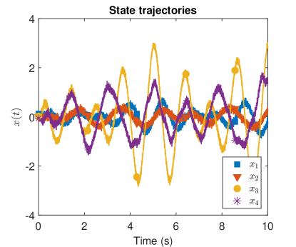
(a) State trajectory.

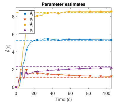
(b) Trajectories of the parameter estimates. Dashed lines represent the ideal values.

Figure 1: Trajectories of the system state and the parameter estimates.

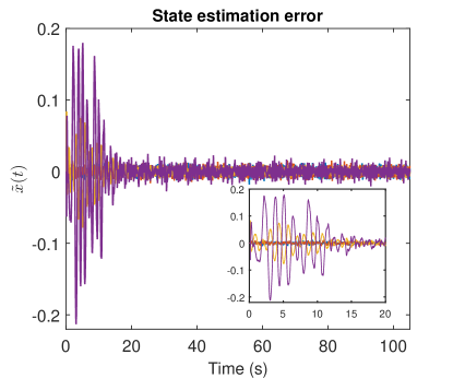
(a) State estimation error.

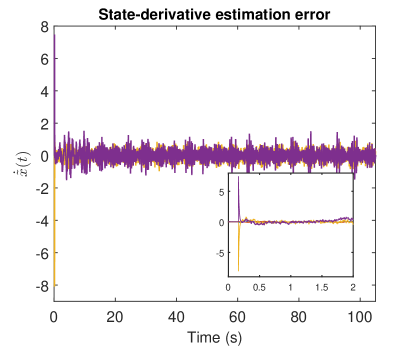
(b) State-derivative estimation error.

Figure 2: Performance of the state-derivative estimator.

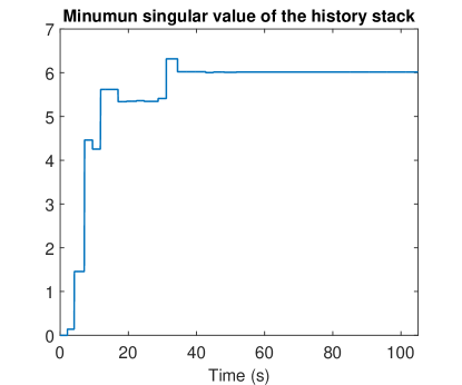
(a) Minimum singular value of the history stack.

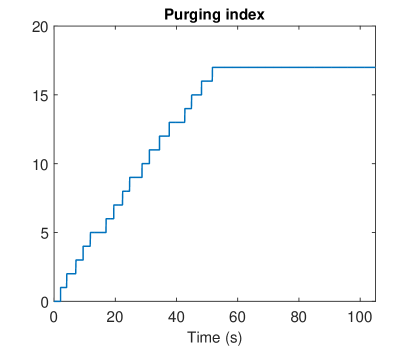
(b) Purging index

Figure 3: Purging index and the minimum singular value for the history stack.

VII Concluding remarks

A concurrent learning-based parameter estimator is developed for a linearly parameterized control-affine nonlinear system. An adaptive observer is employed to generate the state-derivative estimates required for concurrent learning. The developed technique is validated via simulations on a nonlinear system where the state measurements are corrupted by additive Gaussian noise. The simulation results indicate that the developed technique yields better results than numerical differentiation-based CL, even more so as the variance of the additive noise is increased. Even though the simulation results indicate a degree of robustness to measurement noise, the theoretical development does not account for measurement noise.

Measurement noise affects the developed parameter estimator in two ways. An error is introduced in the state-derivative estimates generated using the adaptive observer, and an error is introduced via the history stack since the state measurements recorded in the history stack are corrupted by noise. The former can be addressed if a noise rejecting observer such as a Kalman filter is used to generate the state-derivative estimates. The latter can be addressed by the use of an inherently noise-robust function approximation technique, e.g., a Gaussian process, to approximate the system dynamics. An extension of the developed parameter estimator that is provably robust to measurement noise is a topic for future research.

References

• [1] N. Sureshbabu and J. Farrell, “Wavelet-based system identification for nonlinear control,” IEEE Trans. Autom. Control, vol. 44, no. 2, pp. 412–417, 1999.
• [2] O. Nelles, Nonlinear system identification: from classical approaches to neural networks and fuzzy models.   Springer Science & Business Media, 2001.
• [3] H. Jaeger, “Tutorial on training recurrent neural networks, covering BPTT, RTRL, EKF and the "echo state network" approach,” German National Research Center for Information Technology, Bremen, Tech. Rep. 159, 2002.
• [4] P. P. Angelov and D. P. Filev, “An approach to online identification of takagi-sugeno fuzzy models,” IEEE Trans. Syst. Man Cybern. Part B Cybern., vol. 34, no. 1, pp. 484–498, 2004.
• [5] M. A. Duarte and K. Narendra, “Combined direct and indirect approach to adaptive control,” IEEE Trans. Autom. Control, vol. 34, no. 10, pp. 1071–1075, Oct 1989.
• [6] M. Krstić, P. V. Kokotović, and I. Kanellakopoulos, “Transient-performance improvement with a new class of adaptive controllers,” Syst. Control Lett., vol. 21, no. 6, pp. 451 – 461, 1993.
• [7] E. Lavretsky, “Combined/composite model reference adaptive control,” IEEE Trans. Autom. Control, vol. 54, no. 11, pp. 2692–2697, Nov 2009.
• [8] G. V. Chowdhary and E. N. Johnson, “Theory and flight-test validation of a concurrent-learning adaptive controller,” J. Guid. Control Dynam., vol. 34, no. 2, pp. 592–607, March 2011.
• [9] H. Fukushima, T.-H. Kim, and T. Sugie, “Adaptive model predictive control for a class of constrained linear systems based on the comparison model,” Automatica, vol. 43, no. 2, pp. 301 – 308, 2007.
• [10] V. Adetola, D. DeHaan, and M. Guay, “Adaptive model predictive control for constrained nonlinear systems,” Syst. Control Lett., vol. 58, no. 5, pp. 320 – 326, 2009.
• [11] G. Chowdhary, M. Mühlegg, J. How, and F. Holzapfel, “Concurrent learning adaptive model predictive control,” in Advances in Aerospace Guidance, Navigation and Control, Q. Chu, B. Mulder, D. Choukroun, E.-J. van Kampen, C. de Visser, and G. Looye, Eds.   Springer Berlin Heidelberg, 2013, pp. 29–47.
• [12] A. Aswani, H. Gonzalez, S. S. Sastry, and C. Tomlin, “Provably safe and robust learning-based model predictive control,” Automatica, vol. 49, no. 5, pp. 1216 – 1226, 2013.
• [13] P. Abbeel, M. Quigley, and A. Y. Ng, “Using inaccurate models in reinforcement learning,” in Int. Conf. Mach. Learn.   New York, NY, USA: ACM, 2006, pp. 1–8.
• [14] D. Mitrovic, S. Klanke, and S. Vijayakumar, “Adaptive optimal feedback control with learned internal dynamics models,” in From Motor Learning to Interaction Learning in Robots, ser. Studies in Computational Intelligence, O. Sigaud and J. Peters, Eds.   Springer Berlin Heidelberg, 2010, vol. 264, pp. 65–84.
• [15] M. P. Deisenroth and C. E. Rasmussen, “Pilco: A model-based and data-efficient approach to policy search,” in Int. Conf. Mach. Learn., 2011, pp. 465–472.
• [16] R. Kamalapurkar, P. Walters, and W. E. Dixon, “Concurrent learning-based approximate optimal regulation,” in Proc. IEEE Conf. Decis. Control, Florence, IT, Dec. 2013, pp. 6256–6261.
• [17] G. Chowdhary, “Concurrent learning adaptive control for convergence without persistencey of excitation,” Ph.D. dissertation, Georgia Institute of Technology, December 2010.
• [18] G. Chowdhary, T. Yucelen, M. Mühlegg, and E. N. Johnson, “Concurrent learning adaptive control of linear systems with exponentially convergent bounds,” Int. J. Adapt. Control Signal Process., vol. 27, no. 4, pp. 280–301, 2013.
• [19] M. Mühlegg, G. Chowdhary, and E. Johnson, “Concurrent learning adaptive control of linear systems with noisy measurements,” in Proc. AIAA Guid. Navig. Control Conf., 2012.
• [20] A. Gelb, Applied optimal estimation.   The MIT press, 1974.
• [21] B. Reish and G. Chowdhary, “Concurrent learning adaptive control for systems with unknown sign of control effectiveness,” in Proc. IEEE Conf. Decis. Control, 2014, pp. 4131–4136.
• [22] P. Patre, W. Mackunis, K. Dupree, and W. E. Dixon, “Modular adaptive control of uncertain Euler-Lagrange systems with additive disturbances,” IEEE Trans. Autom. Control, vol. 56, no. 1, pp. 155–160, 2011.
• [23] H. A. Kingravi, G. Chowdhary, P. A. Vela, and E. N. Johnson, “Reproducing kernel hilbert space approach for the online update of radial bases in neuro-adaptive control,” IEEE Trans. Neural Netw. Learn. Syst., vol. 23, no. 7, pp. 1130–1141, 2012.
• [24] P. A. Ioannou and P. V. Kokotovic, Eds., Adaptive Systems with Reduced Models, ser. Lecture Notes in Control and Information Sciences.   Springer Berlin Heidelberg, 1983, vol. 47, ch. 5. Adaptive control in the presence of disturbances, pp. 81–90.
• [25] H. K. Khalil, Nonlinear Systems, 3rd ed.   Upper Saddle River, NJ, USA: Prentice Hall, 2002.