Stable Emergent Universe – A Creation without Big-Bang

Abstract

Based on an earlier introduced new class of generalized gravity-matter models defined in terms of two independent non-Riemannian volume forms (alternative generally covariant integration measure densities) on the space-time manifold, we derive an effective “Einstein-frame” theory featuring the following remarkable properties: (i) We obtain effective potential for the cosmological scalar field possessing two infinitely large flat regions which allows for a unified description of both early universe inflation as well as of present dark energy epoch; (ii) For a specific parameter range the model possesses a non-singular stable “emergent universe” solution which describes an initial phase of evolution that precedes the inflationary phase.

1 Introduction

Here we present a unified cosmological scenario of “k-essence” type (Chiba et.al. 2000; Armendariz-Picon et.al. 2000, 2001; Chiba 2002) where both an inflation phase of the “early” universe and a slowly accelerated phase of the “late” universe do appear naturally from the existence of two infinitely large flat regions in the effective potential of the pertinent cosmological scalar field, which we derive systematically from a well-defined Lagrangian action principle. Our starting point is the earlier proposed (Guendelman et.al. 2015a, 2015b) new kind of globally Weyl-scale invariant gravity-matter action within the first-order (Palatini) approach formulated in terms of two different non-Riemannian volume forms (integration measures on the spacetime manifold). The latter are constructed in terms of auxiliary maximal rank antisymmetric tensor gauge fields called “measure gauge fields”. The cosmological scalar field has kinetic terms coupled to both non-Riemannian measures, and in addition to the scalar curvature term $R$ also an $R^{2}$ term is included (which is similarly allowed by global Weyl-scale invariance). Scale invariance is spontaneously broken upon solving the equations of motion for the auxiliary measure gauge fields due to the appearance of two arbitrary dimensionful integration constants.

In the physical Einstein frame we obtain an effective k-essence (Chiba et.al. 2000; Armendariz-Picon et.al. 2000, 2001; Chiba 2002) type of theory, where the effective scalar field potential has two infinitely-large flat regions. The latter correspond to the two accelerating phases of the universe – the inflationary early universe and the present “late”universe.

Another remarkable result we obtain within the flat region of the effective scalar potential corresponding to the early universe is the appearance of an additional phase that precedes the inflation and describes a non-singular no Big Bang creation of the universe. It is of an “emergent universe” type (Ellis & Maartens 2004; Ellis et.al. 2004; Mulryne et.al. 2005) i.e., the universe starts as a static Einstein universe, the scalar field rolls with a constant speed through a flat region and there is a domain in the parameter space of the theory where such non-singular solution exists and is stable.

Concluding the introductory remarks let us point out that the formalism employing alternative non-Riemannian volume forms in (generalized) gravity triggers a number of physically interesting phenomena in spite of the “pure-gauge” nature of the auxiliary measure gauge fields. Apart from a new type of “quintessential inflation” scenario in cosmology describing both the “early” and “late” universe in terms of a single scalar field and the uncovery of a stable initial non-singular “emergent” universe evolutionary phase (Guendelman et.al. 2015a, 2015b; and here below) we have: (i) new generic mechanism of dynamical generation of cosmological constant; (ii) new mechanism of dynamical spontaneous breakdown of supersymmetry in supergravity (Guendelman et.al. 2014, 2015c); (iii) Coupling of non-Riemannian volume-form gravity-matter theories to a special non-standard kind of nonlinear gauge system containing the square-root of standard Maxwell/Yang-Mills Lagrangian yields charge confinement/deconfinement phases associated with gravitational electrovacuum “bag” (Guendelman et.al. 2015d).

2 Generalized Gravity-Matter Models Built With Two Independent Non-Riemannian Volume-Forms

Our starting point is a generalized modified-measure gravity-matter theory constructed in terms of two different non-Riemannian volume-forms (employing first-order Palatini formalism, and using units where $G_{\rm Newton}=1/16\pi$) (Guendelman et.al. 2015a, 2015b):

$$S=\int d^{4}x\,\Phi_{1}(A)\Bigl{[}R+L^{(1)}\Bigr{]}$$

$$+\int d^{4}x\,\Phi_{2}(B)\Bigl{[}L^{(2)}+\epsilon R^{2}+\frac{\Phi(H)}{\sqrt{-g}}\Bigr{]}\;.$$ (1)

Here and below the following notations are used:

• $\Phi_{1}(A)$ and $\Phi_{2}(B)$ are two independent non-Riemannian volume-forms:

  $$\Phi_{1}(A)=\frac{1}{3!}\varepsilon^{\mu\nu\kappa\lambda}\partial_{\mu}A_{\nu\kappa\lambda}\;\;,\;\;\Phi_{2}(B)=\frac{1}{3!}\varepsilon^{\mu\nu\kappa\lambda}\partial_{\mu}B_{\nu\kappa\lambda}\;.$$ (2)

• $\Phi(H)$ is the dual field-strength of a third auxiliary gauge field $H_{\mu\nu\lambda}$:

  $$\Phi(H)=\frac{1}{3!}\varepsilon^{\mu\nu\kappa\lambda}\partial_{\mu}H_{\nu\kappa\lambda}\;,$$ (3)

  whose presence is essential for the consistency of (1).

• $R=g^{\mu\nu}R_{\mu\nu}(\Gamma)$ and $R_{\mu\nu}(\Gamma)$ are the scalar curvature and the Ricci tensor in the first-order (Palatini) formalism, where the affine connection $\Gamma^{\mu}_{\nu\lambda}$ is a priori independent of the metric $g_{\mu\nu}$. In the second action term in (1) we have added a $R^{2}$ gravity term (again in the Palatini form).

• $L^{(1,2)}$ denote two different Lagrangians of a single scalar matter field (“dilaton” or “inflaton”) of the form:

  $$L^{(1)}=-\frac{1}{2}g^{\mu\nu}\partial_{\mu}\varphi\partial_{\nu}\varphi-V(\varphi)\;\;,\;\;V(\varphi)=f_{1}e^{-\alpha\varphi}\;,$$ (4)

  $$L^{(2)}=-\frac{b}{2}e^{-\alpha\varphi}g^{\mu\nu}\partial_{\mu}\varphi\partial_{\nu}\varphi+U(\varphi)\;\;,\;\;U(\varphi)=f_{2}e^{-2\alpha\varphi}\;,$$ (5)

  where $\alpha,f_{1},f_{2}$ are dimensionful positive parameters, whereas $b$ is a dimensionless one.

The action (1) possesses a global Weyl-scale invariance:

$$g_{\mu\nu}\to\lambda g_{\mu\nu}\;,\;\Gamma^{\mu}_{\nu\lambda}\to\Gamma^{\mu}_{\nu\lambda}\;,\;\varphi\to\varphi+\frac{1}{\alpha}\ln\lambda\;,$$ (6)

$$A_{\mu\nu\kappa}\to\lambda A_{\mu\nu\kappa}\;,\;B_{\mu\nu\kappa}\to\lambda^{2}B_{\mu\nu\kappa}\;,\;H_{\mu\nu\kappa}\to H_{\mu\nu\kappa}\;.$$

The equations of motion w.r.t. affine connection $\Gamma^{\mu}_{\nu\lambda}$ resulting from the action (1) yield the following solution for the latter:

$$\Gamma^{\mu}_{\nu\lambda}=\Gamma^{\mu}_{\nu\lambda}({\bar{g}})=\frac{1}{2}{\bar{g}}^{\mu\kappa}\left(\partial_{\nu}{\bar{g}}_{\lambda\kappa}+\partial_{\lambda}{\bar{g}}_{\nu\kappa}-\partial_{\kappa}{\bar{g}}_{\nu\lambda}\right)\;,$$ (7)

as a Levi-Civita connection corresponding to the Weyl-rescaled metric ${\bar{g}}_{\mu\nu}$:

$${\bar{g}}_{\mu\nu}=(\chi_{1}+2\epsilon\chi_{2}R)g_{\mu\nu}\;\;,\;\;\chi_{1}\equiv\frac{\Phi_{1}(A)}{\sqrt{-g}}\;\;,\;\;\chi_{2}\equiv\frac{\Phi_{2}(B)}{\sqrt{-g}}\;.$$ (8)

Transition from the original metric $g_{\mu\nu}$ to ${\bar{g}}_{\mu\nu}$ accomplishes the passage to the physical “Einstein-frame”, where the gravity equations of motion acquire the standard Einstein’s form $~{}R_{\mu\nu}({\bar{g}})-\frac{1}{2}{\bar{g}}_{\mu\nu}R({\bar{g}})=\frac{1}{2}T^{\rm eff}_{\mu\nu}$ with an appropriate effective matter energy-momentum tensor defined in terms of an effective Einstein-frame matter Lagrangian $L_{\rm eff}$ (see (13) below).

Variation of the action (1) w.r.t. auxiliary tensor gauge fields $A_{\mu\nu\lambda}$, $B_{\mu\nu\lambda}$ and $H_{\mu\nu\lambda}$ yields the equations:

$$\partial_{\mu}\Bigl{[}R+L^{(1)}\Bigr{]}=0\;,\;\partial_{\mu}\Bigl{[}L^{(2)}+\epsilon R^{2}+\frac{\Phi(H)}{\sqrt{-g}}\Bigr{]}=0\;,\;\partial_{\mu}\Bigl{(}\frac{\Phi_{2}(B)}{\sqrt{-g}}\Bigr{)}=0$$

whose solutions read:

$$\frac{\Phi_{2}(B)}{\sqrt{-g}}\equiv\chi_{2}={\rm const}\;\;,\;\;R+L^{(1)}=-M_{1}={\rm const}\;,$$

$$L^{(2)}+\epsilon R^{2}+\frac{\Phi(H)}{\sqrt{-g}}=-M_{2}={\rm const}\;.$$ (10)

Here $M_{1}$ and $M_{2}$ are arbitrary dimensionful and $\chi_{2}$ arbitrary dimensionless integration constants.

The first integration constant $\chi_{2}$ in (10) preserves global Weyl-scale invariance (6) whereas the appearance of the second and third integration constants $M_{1},\,M_{2}$ signifies dynamical spontaneous breakdown of global Weyl-scale invariance under (6) due to the scale non-invariant solutions (second and third ones) in (10).

To elucidate the physical meaning of the three arbitrary integration constants $M_{1},\,M_{2},\,\chi_{2}$ we used in Refs.(Guendelman et.al. 2015b, 2014, 2015c) the canonical Hamiltonian formalism. Namely, $M_{1},\,M_{2},\,\chi_{2}$ are identified as conserved Dirac-constrained canonical momenta conjugated to the “magnetic” components of the auxiliary maximal rank antisymmetric tensor gauge fields $A_{\mu\nu\lambda},B_{\mu\nu\lambda},H_{\mu\nu\lambda}$ entering the original non-Riemannian volume-form action (1). The rest (“electric”) components of $A_{\mu\nu\lambda},B_{\mu\nu\lambda},H_{\mu\nu\lambda}$ appear as Lagrange multipliers for the above Dirac constraints.

Varying (1) w.r.t. $g_{\mu\nu}$ and using relations (8), (10) we arrive at the standard form of Einstein equations for the rescaled metric ${\bar{g}}_{\mu\nu}$, i.e., the “Einstein-frame” equations:

$$R_{\mu\nu}({\bar{g}})-\frac{1}{2}{\bar{g}}_{\mu\nu}R({\bar{g}})=\frac{1}{2}T^{\rm eff}_{\mu\nu}$$ (11)

with energy-momentum tensor corresponding according to the standard definition:

$$T^{\rm eff}_{\mu\nu}=g_{\mu\nu}L_{\rm eff}-2\frac{{\partial{}}}{{\partial{g^{\mu\nu}}}}L_{\rm eff}$$ (12)

to the following effective (Einstein-frame) scalar field Lagrangian of non-canonical “k-essence” (kinetic quintessence) type (Chiba et.al. 2000; Armendariz-Picon et.al. 2000, 2001; Chiba 2002) (here $X\equiv-\frac{1}{2}{\bar{g}}^{\mu\nu}\partial_{\mu}\varphi\partial_{\nu}\varphi$ denotes the scalar kinetic term):

$$L_{\rm eff}=A(\varphi)X+B(\varphi)X^{2}-U_{\rm eff}(\varphi)\;,$$ (13)

where (recall $V=f_{1}e^{-\alpha\varphi}$ and $U=f_{2}e^{-2\alpha\varphi}$):

$$A(\varphi)\equiv 1\!+\!\Bigl{[}\frac{1}{2}be^{-\alpha\varphi}\!-\!\epsilon(V-M_{1})\Bigr{]}\frac{V-M_{1}}{U+M_{2}+\epsilon(V-M_{1})^{2}}\phantom{aa}$$ (14)

$$B(\varphi)\equiv\chi_{2}\frac{\epsilon\Bigl{[}U+M_{2}+(V-M_{1})be^{-\alpha\varphi}\Bigr{]}-\frac{1}{4}b^{2}e^{-2\alpha\varphi}}{U+M_{2}+\epsilon(V-M_{1})^{2}}\;,\phantom{aaa}$$ (15)

$$U_{\rm eff}(\varphi)\equiv\frac{(V-M_{1})^{2}}{4\chi_{2}\Bigl{[}U+M_{2}+\epsilon(V-M_{1})^{2}\Bigr{]}}\;.\phantom{aaa}$$ (16)

3 Infinitely Large Flat Regions of the Effective Scalar Potential

The effective scalar potential $U_{\rm eff}(\varphi)$ (16) possesses the following remarkable feature – the existence of two infinitely large flat regions as function of $\varphi$ which is an explicit realization of quintessential inflation scenario (Peebles & Vilenkin 1999; Appleby et.al. 2010).

The explicit form of the two flat regions is as follows:

• (-) flat region – for large negative values of $\varphi$:

  $$U_{\rm eff}(\varphi)\simeq U_{(-)}\equiv\frac{f_{1}^{2}/f_{2}}{4\chi_{2}(1+\epsilon f_{1}^{2}/f_{2})}\;,$$ (17)

• (+) flat region – for large positive values of $\varphi$:

  $$U_{\rm eff}(\varphi)\simeq U_{(+)}\equiv\frac{M_{1}^{2}/M_{2}}{4\chi_{2}(1+\epsilon M_{1}^{2}/M_{2})}\;,$$ (18)

The qualitative shape of $U_{\rm eff}(\varphi)$ (16) is depicted on Figs.1 and 2.

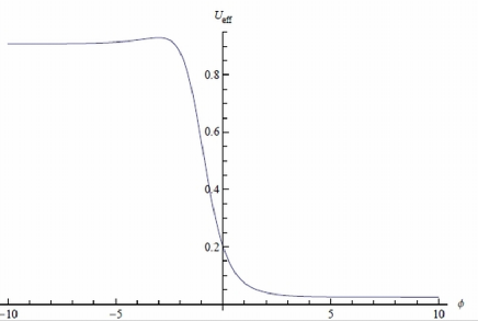
Figure 1: Qualitative shape of the effective scalar potential $U_{\rm eff}$ U-eff as function of $\varphi$ for $M_{1}<0$.

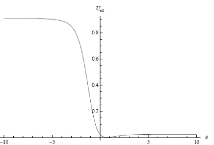
Figure 2: Qualitative shape of the effective scalar potential $U_{\rm eff}$ (16) as function of $\varphi$ for $M_{1}>0$.

The flat regions (17) and (18) correspond to the evolution of early and the late universe, respectively, provided we choose the ratio of the coupling constants in the original scalar potentials versus the ratio of the scale-symmetry breaking integration constants to obey the following strong inequality:

$$\frac{f_{1}^{2}}{f_{2}}\gg\frac{M_{1}^{2}}{M_{2}}\quad,\quad|\epsilon|\frac{M_{1}^{2}}{M_{2}}\ll 1\;.$$ (19)

which makes the vacuum energy density of the early universe $U_{(-)}$ (17) much bigger than that of the late universe $U_{(+)}$ (18)).

If we choose the scales $|M_{1}|\sim M^{4}_{EW}$ and $M_{2}\sim M^{4}_{Pl}$ (Arkani-Hamed et.al. 2000), where $M_{EW},\,M_{Pl}$ are the electroweak and Planck scales, respectively, we are then naturally led to a very small vacuum energy density:

$$U_{(+)}\sim M^{8}_{EW}/M^{4}_{Pl}\sim 10^{-120}M^{4}_{Pl}\;,$$ (20)

which is the right order of magnitude for the present epoch’s vacuum energy density.

On the other hand, if we take the order of magnitude of the coupling constants in the effective potential $f_{1}\sim f_{2}\sim(10^{-2}M_{Pl})^{4}$, then the order of magnitude of the vacuum energy density of the early universe becomes:

$$U_{(-)}\sim f_{1}^{2}/f_{2}\sim 10^{-8}M_{Pl}^{4}\;,$$ (21)

which conforms to the Planck Collaboration data (Adam et.al. 2015) implying the energy scale of inflation to be of order $10^{-2}M_{Pl}$.

4 Non-Singular Stable “Emergent Universe” Solution

We start with the Friedman equations, see e.g. (Weinberg 1972):

$$\frac{\stackrel{{\scriptstyle..}}{{a}}}{a}=-\frac{1}{12}(\rho+3p)\quad,\quad H^{2}+\frac{K}{a^{2}}=\frac{1}{6}\rho\quad,\;\;H\equiv\frac{\stackrel{{\scriptstyle.}}{{a}}}{a}\;,$$ (22)

describing the universe’ evolution. In the present case with “Einstein frame” effective scalar field action (13) the energy density $\rho$ and the pressure $p$ of the scalar field $\varphi=\varphi(t)$ read explicitly:

$$\rho=\frac{1}{2}A(\varphi)\stackrel{{\scriptstyle.}}{{\varphi}}^{2}+\frac{3}{4}B(\varphi)\stackrel{{\scriptstyle.}}{{\varphi}}^{4}+U_{\rm eff}(\varphi)\;,$$ (23)

$$p=\frac{1}{2}A(\varphi)\stackrel{{\scriptstyle.}}{{\varphi}}^{2}+\frac{1}{4}B(\varphi)\stackrel{{\scriptstyle.}}{{\varphi}}^{4}-U_{\rm eff}(\varphi)\;.$$ (24)

$H$ is the Hubble parameter and $K$ denotes the Gaussian curvature of the spacial section in the Friedman-Lemaitre-Robertson-Walker metric, see e.g. (Weinberg 1972):

$$ds^{2}=-dt^{2}+a^{2}(t)\Bigl{[}\frac{dr^{2}}{1-Kr^{2}}+r^{2}(d\theta^{2}+\sin^{2}\theta d\phi^{2})\Bigr{]}\;.$$ (25)

“Emergent universe” is defined as a solution of the Friedman Eqs.(22) subject to the condition on the Hubble parameter $H$:

$$H=0\;\;\to\;\;a(t)=a_{0}={\rm const}\,,\;\;\rho+3p=0\;,$$

$$\frac{K}{a_{0}^{2}}=\frac{1}{6}\rho~{}(={\rm const})\;,$$ (26)

with $\rho$ and $p$ as in (23)-(24). Here $K=1$ (“Einstein universe”).

The “emergent universe” condition (26) implies that the $\varphi$-velocity $\stackrel{{\scriptstyle.}}{{\varphi}}\equiv\stackrel{{\scriptstyle.}}{{\varphi}}_{0}$ is time-independent and satisfies the bi-quadratic algebraic equation:

$$\frac{3}{2}B_{(-)}\stackrel{{\scriptstyle.}}{{\varphi}}_{0}^{4}+2A_{(-)}\stackrel{{\scriptstyle.}}{{\varphi}}_{0}^{2}-2U_{(-)}=0\;,$$ (27)

where $A_{(-)},\,B_{(-)},\,U_{(-)}$ are the limiting values on the $(-)$ flat region of $A(\varphi),\,B(\varphi),\,U_{\rm eff}(\varphi)$ (14)-(16).

The solution of Eq.(27) reads:

$$\stackrel{{\scriptstyle.}}{{\varphi}}_{0}^{2}=-\frac{2}{3B_{(-)}}\Bigl{[}A_{(-)}\mp\sqrt{A_{(-)}^{2}+3B_{(-)}U_{(-)}}\Bigr{]}\;.$$ (28)

and, thus, the “emergent universe” is characterized with finite initial Friedman factor and density:

$$a_{0}^{2}=\frac{6K}{\rho_{0}}\quad,\quad\rho_{0}=\frac{1}{2}A_{(-)}\stackrel{{\scriptstyle.}}{{\varphi}}_{0}^{2}+\frac{3}{4}B_{(-)}\stackrel{{\scriptstyle.}}{{\varphi}}_{0}^{4}+U_{(-)}\;,$$ (29)

with $\stackrel{{\scriptstyle.}}{{\varphi}}_{0}^{2}$ as in (28).

Analysis of stability of the “emergent universe” solution (29) yields a harmonic oscillator type equation for the perturbation of the Friedman factor $\delta a$:

$$\delta\stackrel{{\scriptstyle..}}{{a}}+\omega^{2}\delta a=0\;,$$ (30)

with a “frequency” squared:

$$\omega^{2}\equiv\frac{2}{3}\rho_{0}\,\frac{\sqrt{A_{(-)}^{2}+3B_{(-)}U_{(-)}}}{A_{(-)}-2\sqrt{A_{(-)}^{2}+3B_{(-)}U_{(-)}}}\;.$$ (31)

Thus, stability condition $\omega^{2}>0$ implies the following constraint on the coupling parameters:

$${\rm max}\Bigl{\{}-2\,,\,-8\bigl{(}1+3\epsilon f_{1}^{2}/f_{2}\bigr{)}\Bigl{[}1-\sqrt{1-\frac{1}{4\bigl{(}1+3\epsilon f_{1}^{2}/f_{2}\bigr{)}}}\Bigr{]}\Bigr{\}}$$

$$<b\frac{f_{1}}{f_{2}}<-1\;.$$ (32)

Since the ratio $\frac{f_{1}^{2}}{f_{2}}$ proportional to the height of the $(-)$ flat region of the effective scalar potential, i.e., the vacuum energy density in the early universe, must be large (cf. (19)), we find that the lower end of the interval in (32) is very close to the upper end, i.e., $b\frac{f_{1}}{f_{2}}\simeq-1$.

From Eqs.(28)-(29) we obtain an inequality satisfied by the initial energy density $\rho_{0}$ in the emergent universe:

$$U_{(-)}<\rho_{0}<2U_{(-)}\;,$$ (33)

which together with the estimate of the order of magnitude for $U_{(-)}$ (21) implies order of magnitude for the initial Friedman factor:

$$a_{0}^{2}\sim 10^{-8}KM_{Pl}^{-2}$$ (34)

($K$ being the Gaussian curvature of the spacial section).

5 Concluding Remarks

In Ref.(Guendelman et.al. 2015) the implications resulting from the present model for the ratio $r$ of tensor-to-scalar perturbations were studied. It was found that very small values of the coupling parameter $\alpha$ (appearing in the initial scalar potentials (4)-(5)) yield small values for $r$ (e.g., the value $\alpha\simeq 10^{-20}$ correspond to $r\simeq 0.017$) which are well supported by Planck data.

Furthermore, in Ref.(Guendelman et.al. 2015) the system of evolutionary equations (the Friedman ones (22) plus the scalar field equations of motion resulting from the effective “k-essence” Lagrangian (13)) was studied in some detail using the methods of autonomous dynamical systems. A numerical evidence was found for the existence of a short transitional phase of “super-inflation” (Labrana 2013) connecting the “emergent” and the “slow-roll” inflationary phases.

Few additional questions can be studied, for example the problem of reheating, which one may worry about. The reason is that the effective scalar field (inflaton) potential may either lack a minimum (Fig.1 above) or the pertinent minimum may be too shallow (Fig.2 above) so that this appears to imply the absence of an oscillatory behavior for the standard reheating scenario. It is possible to introduce a curvaton field, which takes care of reheating and primordial perturbations – this can be done in a scale-invariant way (Guendelman & Ramon 2015).

Another interesting subject concerns the quantum stability, extending the proof of classical stability, of the “emergent universe” solution to the quantum regime (del Campo et.al 2015).

To recapitulate, let us list the main features illustrating the impact of non-Riemannian volume-forms in generally-covariant theories:

• Non-Riemannian volume-form formalism in gravity/matter theories (i.e., employing alternative non-Riemannian reparametrization covariant integration measure densities on the spacetime manifold) naturally generates a dynamical cosmological constant as an arbitrary dimensionful integration constant.

• Employing two different non-Riemannian volume-forms leads to the construction of a new class of gravity-matter models, which produce an effective scalar potential with two infinitely large flat regions. This allows for a unified description of both early universe inflation as well as of present dark energy epoch.

• A remarkable feature is the existence of a stable initial phase of non-singular universe creation preceding the inflationary phase – “emergent universe” without “Big-Bang”.

Further very interesting features of gravity-matter theories built with non-Riemannian spacetime volume-forms include:

• Within non-Riemannian-modified-measure minimal $N=1$ supergravity the dynamically generated cosmological constant triggers spontaneous supersymmetry breaking and mass generation for the gravitino, i.e., supersymmetric Brout-Englert-Higgs effect (Guendelman et.al. 2014, 2015c). Applying the same non-Riemannian volume-form formalism to anti-de Sitter supergravity allows to produce simultaneously a very large physical gravitino mass and a very small positive observable cosmological constant (Guendelman et.al. 2014, 2015c) in accordance with modern cosmological scenarios for slowly expanding universe of the present epoch (Riess et.al. 1998,2004; Perlmutter et.al. 1999).

• Adding interaction with a special nonlinear (“square-root” Maxwell) gauge field (known to describe charge confinement in flat spacetime) produces various phases with different strength of confinement and/or with deconfinement, as well as gravitational electrovacuum “bags” partially mimicking the properties of MIT bags and solitonic constituent quark models (for details, see Ref.(Guendelman et.al. 2015d)).

\acknowledgements

E.G., E.N. and S.P. gratefully acknowledge support of our collaboration through the academic exchange agreement between the Ben-Gurion University in Beer-Sheva, Israel, and the Bulgarian Academy of Sciences. R.H. was supported by Comisión Nacional de Ciencias y Tecnología of Chile through FONDECYT Grant 1130628 and DI-PUCV 123.724. P.L. was supported by Dirección de Investigación de la Universidad del Bío-Bío through grants GI121407/VBC and 141407 3/R. S.P. and E.N. have received partial support from European COST Actions MP-1210 and MP-1405, respectively, as well as from Bulgarian NSF Grant DFNI-T02/6.

References

- [1] Adam R. et.al. (Planck Collaboration) 2015, Astronomy & Astrophysics http://dx.doi.org/10.1051/0004-6361/201425034 (arXiv:1409.5738 [astro-ph.CO]).
- [2] Appleby S.A., Battye R.A. & Starobinsky A.A. 2010, JCAP 1006 005 (arXiv:0909.1737 [astro-ph]).
- [3] Arkani-Hamed N., Hall L.J., Kolda C. & Murayama H. 2000, Phys. Rev. Lett. 85 4434-4437 (astro-ph/0005111).
- [4] Armendariz-Picon C., Mukhanov V. & Steinhardt P. 2000, Phys. Rev. Lett. 85 4438 (arXiv:astro-ph/0004134).
- [5] Armendariz-Picon C., Mukhanov V. & Steinhardt P. 2001, Phys. Rev. D63 103510 (arXiv:astro-ph/0006373)
- [6] Chiba T., Okabe T.& Yamaguchi M. 2000, Phys. Rev. D62 023511 (arXiv:astro-ph/9912463),
- [7] Chiba T. 2002, Phys. Rev. D66 063514 (arXiv:astro-ph/0206298).
- [8] Del Campo S., Guendelman E., Herrera R. and Labrana P. 2015, work in progress.
- [9] Ellis G.F.R. & Maartens R. 2004, Class. Quant. Grav. 21 223 (gr-qc/0211082).
- [10] Ellis G.F.R., Murugan J. & Tsagas C.G. 2004, Class. Quant. Grav. 21 233 ( arxiv:gr-qc/0307112).
- [11] Guendelman E., Herrera R., Labrana P., Nissimov E. & Pacheva S. 2015, Gen. Rel. Grav. 47 art.10 (arXiv:1408.5344v4 [gr-qc]).
- [12] Guendelman E., Nissimov E. & Pacheva S. 2015, in Eight Mathematical Physics Meeting, pp.93-103, B. Dragovic and I. Salom (eds.), Belgrade Inst. Phys. Press (arXiv:1407.6281v4 [hep-th]).
- [13] Guendelman E., Nissimov E., Pacheva S. & Vasihoun M. 2014, Bulg. J. Phys. 41 123-129 (arXiv:1404.4733 [hep-th]).
- [14] Guendelman E., Nissimov E., Pacheva S. & Vasihoun M. 2015, in Eight Mathematical Physics Meeting, pp.105-115, B. Dragovic and I. Salom (eds.), Belgrade Inst. Phys. Press (arXiv:1501.05518)
- [15] Guendelman E., Nissimov E. & Pacheva S. 2015, Int. J. Mod. Phys. A30 1550133 (arxiv:1504.01031).
- [16] Guendelman E. & Ramon H. 2015, work in progress.
- [17] Labrana P. 2013, arxiv:1312.6877 [astro-ph.CO].
- [18] Mulryne D.J., Tavakol R., Lidsey J.E. & Ellis G.F.R. 2005, Phys. Rev. D71 123512 (arxiv:astro-ph/0502589).
- [19] Peebles P.J.E. & Vilenkin A. 1999, Phys. Rev. D59 063505.
- [20] Perlmutter S. et.al. (The Supernova Cosmology Project) 1999, Astrophysical Journal 517 565-586 (arXiv:astro-ph/9812133).
- [21] Riess A.G. et.al. (Supernova Search Team) 1998, Astronomical Journal 116 1009-1038 (arXiv:astro-ph/9805201).
- [22] Riess A.G. et.al. 2004, Astrophysical Journal 607 665-687 (arXiv:astro-ph/0402512).
- [23] Starobinsky A. 1980, Phys. Lett. B91 99-102.
- [24] Weinberg S. 1972, “Gravitation and Cosmology – Principles and Applications of the General Theory of Relativity”, John Wiley & Sons, Inc.