A heuristic extended particle 2D-model compatible with quantum mechanics

Abstract

In this paper we propose an extended particle model whose evolution is deterministic. In dimension 2, the extended particle is represented by four points that define a small elastic string that vibrates, alternating between a creation process and an annihilation process.

First we show how the spin and the Heisenberg uncertainty relations emerge from this extended particle. We then show how the complex action associated with this extended particle satisfies, from a generalized principle of least action, a second order complex Hamilton-Jacobi equation. Third, we show that the wave function, which admits this action as a complex phase, satisfies the Schrödinger equation. Finally, we show that the gravity center of this extended particle follows the trajectories proposed by the de Broglie-Bohm interpretation well as the Schrödinger interpretation.

This model is built on two new mathematical concepts we have introduced: complex analytical mechanics on complex-valued functions and a periodic deterministic process.

I Introduction

One of the fundamental reasons for the impossibility of synthesis between quantum mechanics and general relativity is that quantum mechanics is considered non-deterministic while relativity is considered deterministic. Most current approaches to synthesis research, such as string theory Witten or loop quantum gravity theorySmolin ; Rovelli are based on non-deterministic general relativity. The alternative approach is to render quantum mechanics deterministic.

In this paper, we propose an extended model particle whose evolution is deterministic. In dimension 2, the extended particle is represented by four points that define the structure of a small elastic string that vibrates, alternating between a process of creation and a process of annihilation. We then show how the spin and the Heisenberg uncertainty relations emerge from this extended particle.

We subsequently demonstrate how the complex action associated with this extended particle satisfies, from a generalized principle of least action, a second order complex Hamilton-Jacobi equation. We show that the wave function, which admits this action as a complex phase, satisfies the Schrödinger equation. Finally, we show that the gravity center of this extended particle follows the trajectories proposed by the de Broglie-Bohm interpretation as well the Schrödinger interpretation.

This model is built on two new mathematical concepts: complex analytical mechanics on complex-valued functions, which we have introduced Gondran_1999 ; Gondran_2001a ; Gondran_2001c ; GondranHoblos_2003 , and the periodic deterministic process, which we have developedGondran_2001b ; Gondran_2004 .

II An extended particle model and its trajectory

In an orthonormal space $\mathbb{R}^{2}$, let us consider the four vertices of the unit square $u^{1}=\binom{1}{1}$, $u^{2}=\binom{1}{-1}$, $u^{3}=\binom{-1}{-1}$ and $u^{4}=\binom{-1}{1}$. There are two circular permutations of these four vertices, one $s^{+}$ in a clockwise direction, the other $s^{-}$ in the opposite direction. For each of these permutations $s\in S$ and for all $u^{j}$, we have $s^{4}u^{j}=u^{j}$.

We consider an extended particle represented by four points. For each time step $\varepsilon>0$ and for each of the two permutations $s\in S$, the evolution of the four points at time $t=n\varepsilon$ with $n=4q+r$ ( n,q,r integer and $0\leq r\leq 3$), is defined by the real part of the four following discrete $Z_{\varepsilon}^{j}(t)\in\mathbb{C}^{2}$ processes:

$$Z_{\epsilon}^{j}(n\epsilon)=Z_{\epsilon}^{j}\left(n\epsilon-\epsilon\right)+\mathcal{V}(4q\epsilon)\epsilon+\gamma(s^{n}u^{j}-s^{n-1}u^{j})$$ (1)

$$Z_{\epsilon}^{j}(0)=Z_{0}~{}~{}~{}~{}for~{}all~{}j,$$ (2)

where

$$\gamma=(1+i)\sqrt{\frac{\hslash\varepsilon}{4m}},$$

$\mathcal{V}(t)$ corresponds to a continuous complex function, $\hslash$ is the Planck constant, $m$ the mass of the particle, and $Z_{0}$ is a given vector of $\mathbb{C}^{2}.$

Let $\widetilde{Z}_{\epsilon}(t)$ be the solution in $\mathbb{C}^{2}$ of the discret system deined at time $t=n$ $\epsilon$ with $n=4q+r$ $\left(n\text{, }q\text{ and }r\text{ integers and }0\leq r\leq 3\right)$ by:

$$\widetilde{Z}_{\epsilon}(n\epsilon)=\widetilde{Z}_{\epsilon}(n\epsilon-\epsilon)+\mathcal{V}(4q\epsilon)\epsilon$$ (3)

$$\widetilde{Z_{\epsilon}}(0)=Z_{0}.$$ (4)

We then verify that we have at each time $t=n\epsilon$:

$$Z_{\epsilon}^{j}(n\epsilon)=\widetilde{Z_{\varepsilon}}(n\epsilon)+(1+i)\sqrt{\frac{\hslash\varepsilon}{4m}}\left(s^{n}u^{j}-u^{j}\right).$$ (5)

As $s^{4}u^{j}=u^{j}$, we deduce from (5) that $Z_{\epsilon}^{j}(4q\epsilon)=\widetilde{Z}_{\epsilon}(4q\epsilon)$    for all j.

As $\sum^{j=4}_{j=1}s^{n}u^{j}=0$, we deduce from (1) that the process $\widetilde{Z}_{\epsilon}(t)$ is the average of the four processes $Z_{\epsilon}^{j}(t)$. Its real part $\widetilde{X}_{\epsilon}(t)$ can be interpreted as the gravity center of the particle. The position $X_{\epsilon}^{j}(t)$ of each vertex j, the real part of process $Z_{\epsilon}^{j}(t)$, satisfies the equation:

$$X_{\epsilon}^{j}(n\epsilon)=\widetilde{X_{\varepsilon}}(n\epsilon)+\sqrt{\frac{\hslash\varepsilon}{4m}}\left(s^{n}u^{j}-u^{j}\right).$$ (6)

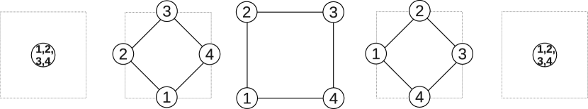
This equation expresses the evolution of the four points of the extended particle in relation to its center of gravity. The evolution of this extended particle over a period of 4 $\epsilon$ is shown in Figure 1.

Figure 1: Evolution of the four points of the extended particle over a period of 4 $\epsilon$ from left to right: points at $4q\epsilon$, in extension at $(4q+1)\epsilon$ and $(4q+2)\epsilon$, then in contraction at $(4q+3)\epsilon$ and $4(q+1)\epsilon$.

We consider that the four points $X_{\epsilon}^{j}(t)$ of the particle define the a string structure. The movement of the four points corresponds to the vibration of the string. At time $t=4q\epsilon$, the four points are at the center of a square and the length of the string at this time is zero. At times $t\neq 4q\epsilon$, it takes an extension. At times $(4q+1)\epsilon$ and $(4q+3)\epsilon$, the four points are at the center of the edges of square. At time $(4q+2)\epsilon$, the four points are on the four vertices of the square. Moreover, this interpretation suggests a creation process between times $t=4q\epsilon$ and $(4q+1)\epsilon$ follows an annihilation process between times $(4q+3)\epsilon$ and $(4q+4)\epsilon$.

The equation (5) leads to $Z_{\epsilon}^{j}(t)=\widetilde{Z}_{\epsilon}(t)+0(\sqrt{\epsilon})$ for all j and all t = n$\epsilon$.

Let $\widetilde{Z}(t)$ be the solution of the classical differential equation:

$$\frac{d\widetilde{Z}(t)}{dt}=\mathcal{V}(t)$$ (7)

$$\widetilde{Z}(0)=Z_{0}.$$ (8)

Because $\mathcal{V}(t)$ is continuously differentiable, we obtain $\widetilde{Z}_{\epsilon}(t)=\widetilde{Z}(t)+0(\epsilon)$ for all $t=n\epsilon$, and then $Z_{\epsilon}^{j}(t)=\widetilde{Z}(t)+0(\sqrt{\epsilon})$. We can deduce

Theorem 1

- Each process $\widetilde{Z}^{j}_{\epsilon}(t)$ continuously converges towards the classical trajectory $\widetilde{Z}(t)$ when $\epsilon\longrightarrow 0^{+}$.

Let us conclude this section with some remarks on the $Z_{\epsilon}^{j}(t)$ processes.

Remark 1

- The four $Z_{\varepsilon}^{j}(t)$ processes looks like to the Nelson stochastic process Nelson_1966 ; Nelson_1985 based on the Wiener process, but unlike the Nelson process they are deterministic. However, despite being deterministic, these processes appear random with respect to the spatial extension of the string because, at time t, the rest modulo 4 of the number $n=$ $\frac{t}{\varepsilon}$ is a pseudorandom number.

Remark 2

- In FeynmannHibbs , Feynmann et Hibbs show that the "important paths" of quantum mechanics, are very irregular and nowhere differentiable. They admit an average velocity $lim_{\Delta t\longrightarrow 0^{+}}\langle\frac{x_{k+1}-x_{k}}{\Delta t}\rangle=v$, but not an average quadratic velocity because $\langle(\frac{x_{k+1}-x_{k}}{\Delta t})^{2}\rangle=\frac{i\hbar}{m\Delta t}$. The four $X_{\varepsilon}^{j}(t)$ processes satisfy the same properties as the Feynmann paths, becoming increasingly irregular and non-differentiabe when $\epsilon\rightarrow 0^{+}$; however, the value of $\varepsilon=\Delta t$, although very small, remains finite.

III Emergence of the spin and Heisenberg uncertainty relations

We have associated with an extended particle four points and one cycle of four instants during the period $T=4\epsilon$. We will assume that the properties of such a particle are the average of the properties of the four points taken on the four instants of the period.

We therefore define the average angular momentum of the extended particle satisfying Equation(6) by:

$$\sigma=E_{n,j}(\sigma^{j}_{n})=\frac{1}{16}\sum_{n=4q}^{4q+3}\sum_{j=1}^{4}\sigma^{j}_{n}$$

with

$$\sigma^{j}_{n}=r^{j}_{n}\wedge p^{j}_{n},~{}~{}~{}~{}r^{j}_{n}=X^{j}_{\varepsilon}(n\varepsilon)=\widetilde{r}_{n}+\sqrt{\frac{\hbar\varepsilon}{4m}}(s^{n}u^{j}-u^{j})$$

and

$$p^{j}_{n}=m\frac{r^{j}_{n+1}-r^{j}_{n}}{\varepsilon}=m\frac{\widetilde{r}_{n+1}-\widetilde{r}_{n}}{\varepsilon}+\sqrt{\frac{\hbar m}{4\varepsilon}}(s^{n+1}u^{j}-s^{n}u^{j}).$$

By using the identity $\sum_{j=1}^{4}s^{n}u^{j}=0$ for all n, we obtain $\sigma=\widetilde{r}\wedge m\widetilde{v}+\frac{1}{16}\hslash\sum_{j=1}^{4}(u^{j}\wedge su^{j})$ with $\widetilde{r}=\frac{1}{4}\sum_{n=4q}^{4q+3}\widetilde{r}_{n}$ and $\widetilde{v}=\widetilde{v}(4q\varepsilon)$. For $s=s^{+}$, we obtain

$$\sigma\equiv\sigma_{z}=m\left(x\widetilde{v}_{y}-y\widetilde{v}_{x}\right)-\frac{\hslash}{2}.$$

We deduce the theorem:

Theorem 2

- For all $\epsilon>0$, the extended particle which corresponds to the real part of process (1)(2), has an average intrinsic angular momentum $s_{z}=-\frac{\hslash}{2}$ for the permutation $s^{+}$ and $s_{z}=+\frac{\hslash}{2}$ for the permutation $s^{-}$.

Let $\widetilde{x}_{\varepsilon}(n\varepsilon)$ be the average position of the particle along the $x$ axis at time $n\varepsilon$ (with $n=4q+r$) and $m\widetilde{v}\left(4q\varepsilon\right)$ the average momentum. The calculation of standard deviations $\triangle x$ and $\Delta p_{x}$ of the position and of the momentum along the $x,$ axis is obtained from the following equations:

$$\langle\Delta x\rangle^{2}=\frac{1}{16}\sum_{n=4q}^{4q+3}\sum_{j=1}^{4}\left(r^{j}_{n}-\widetilde{r}_{n}\right)_{x}^{2}$$

$$\langle\Delta p_{x}\rangle^{2}=\frac{1}{16}\sum_{n=4q}^{4q+3}\sum_{j=1}^{4}\left(p_{n}^{j}-\widetilde{p}_{n}\right)_{x}^{2}$$

with $\widetilde{p}_{n}=m\frac{\widetilde{r}_{n+1}-\widetilde{r}_{n}}{\varepsilon}$. We obtain $\langle\Delta x\rangle=\frac{\hbar\varepsilon}{2m}$ and $\langle\Delta p_{x}\rangle=\frac{\hbar m}{\varepsilon}$. We deduce the theorem:

Theorem 3

- For all $\epsilon>0$ and for all $s$, the extended particle which corresponds to the real part of process (1)(2), satisfies the Heisenberg uncertainty relations:

$$\langle\Delta x\rangle\cdot\langle\Delta p_{x}\rangle=\frac{\hslash}{2}.$$ (9)

Let us consider $f$ a twice differentiable application from $\mathbb{C}^{2}\times\mathbb{R}$ in $\mathbb{C}$. We denote the complex Dynkin operator, introduced by Nottale Nottale under the name of "quantum covariant derivative":

$$D=\frac{\partial}{\partial t}+\mathcal{V}\cdot\triangledown-i\frac{\hslash}{2m}\triangle.$$ (10)

Lemma 4

- For all $\epsilon>0$ and for all $s$, the process $Y_{\epsilon}(t)$ is defined by:

$$Y_{\epsilon}\left(t\right)=Ef(Z_{\epsilon}^{j}\left(t\right),t)=\frac{1}{4}\ \sum_{j}\left(f\left(Z_{\epsilon}^{j}\left(t\right),t\right)\right)$$ (11)

with $Z_{\epsilon}^{j}\left(t\right)$ defined by (1)and (2), satisfies for all $t=4q\varepsilon$ (q integer):

$$Y_{\epsilon}(t)-Y_{\epsilon}\left(t-\varepsilon\right)=Df\left(\widetilde{Z}\left(t\right),t\right)\epsilon+0\left(\epsilon^{2}\right).$$ (12)

Proof: First, we have $Y_{\epsilon}\left(4q\epsilon\right)=f\left(\widetilde{Z}\left(4q\epsilon\right),4q\epsilon\right)$. Using (5) and $\sum_{j}s^{n}u^{j}=0$, we find for all $t=n\epsilon$

$$Ef(Z_{\epsilon}^{j}\left(t\right),t)=f(\widetilde{Z}_{\epsilon}(t),t)+\frac{i\hslash}{4m}\epsilon E\left\{\sum_{k,l}\frac{\partial^{2}f(\widetilde{Z}_{\epsilon}(t),t)}{\partial x_{k}\partial x_{l}}\left(s^{n}u^{j}-u^{j}\right)_{k}\left(s^{n}u^{j}-u^{j}\right)_{l}\right\}+0\left(\epsilon^{2}\right).$$

For $n=4q-1$, $E(s^{n}u^{j}-u^{j})_{k}(s^{n}u^{j}-u^{j})_{l}=\frac{4+4}{4}\delta_{kl}$ and the calculation of the last term of $Ef(Z_{\epsilon}^{j}\left(t\right),t)$ yields $\frac{i\hslash}{4m}\epsilon 2\Delta f$. Then we deduce:

$$Y_{\epsilon}\left(4q\epsilon-\epsilon\right)=f(\widetilde{Z}_{\epsilon}(4q\epsilon-\epsilon),4q\epsilon-\epsilon)+i\frac{\hslash}{2m}\epsilon\Delta f(\widetilde{Z}_{\epsilon}(4q\epsilon-\epsilon),4q\epsilon-\epsilon)+0\left(\epsilon^{2}\right).$$

Hence, the development to first order of $f(\widetilde{Z}_{\epsilon}(4q\epsilon-\epsilon),4q\epsilon-\epsilon)$ leads to equation (12).$\Box$

IV Second order Complex Hamilton-Jacobi equation

We will show that the evolution of the process $Z_{\varepsilon}^{j}(t)$ defined by the equations (1)(2), is also given by a second order complex Hamilton-Jacobi equation. To do this, we use a complex analytical mechanics and a generalized principle of least action. The complex analytical mechanics is a generalization of classic analytical mechanics but with objects having a complex position $Z(t)\in\mathbb{C}^{2}$ and a complex velocity $\mathcal{V}\left(t\right)\in\mathbb{C}^{2}$. We use the complex minimum of a complex function and the complex Minplus analysis introduced in Gondran_1999 ; Gondran_2001a ; Gondran_2001c ; GondranHoblos_2003 . We recall the principle in the following definitions.

Definition 1

- For a complex function $f\left(Z\right)=f\left(X+iY\right)$ from $\mathbb{C}^{n}$ in $\mathbb{C}$ such as $f\left(Z\right)=P\left(X,Y\right)+iQ\left(X,Y\right)$, we define the complex minimun, if it exists, by $\min\left\{f\left(Z\right)/Z\in\mathbb{C}^{n}\right\}=f\left(Z_{0}\right)$ where $\left(X_{0},Y_{0}\right)$ is a saddle point of $P\left(X,Y\right)$: $P\left(X_{0},Y\right)\leq P\left(X_{0},Y_{0}\right)\leq P\left(X,Y_{0}\right)$ $\forall(X,Y)\in R^{n}\times R^{n}$.

A complex function $f\left(Z\right)$ is (strictly) convex if $P\left(X,Y\right)$ is (strictly) convex in $X$ and (strictly) concave in $Y$.

If $f\left(Z\right)$ is a holomorphic function, then a necessary condition for $Z_{0}$ to be a minimum of $f(Z)$ in $\mathbb{C}^{n}$ is $\nabla f(Z)=0$. It is sufficient if $f(Z)$ is also convex.

Using the classical Lagrange function $L(x,\dot{x},t)$, an analytical function in $x$ and $\dot{x}$, we define the complex Lagrange function $L(Z,\mathcal{V},t)$.

Definition 2

- With all complex and strictly convex functions $f(Z)$, we associate a complex Fenchel-Legendre transform $\widehat{f}\left(P\right)$ defined by:

$$\widehat{f}\left(P\right)=\underset{Z\in\mathbb{C}^{n}}{\mathit{\max}}\left(P.Z-f\left(Z\right)\right)$$

Before presenting our generalization of the principle of least action for our extended particle model, let us recall this principle for the definition of the Hamilton-Jacobi action in the classical case. At time 0, an initial action $S^{0}(\textbf{x})$, a function of $\mathbb{R}^{n}$ in $\mathbb{R}$ is given. This initial action corresponds to the initial velocity field $\textbf{v}_{0}(\textbf{x})=\nabla S^{0}(\textbf{x})/m$.

The Hamilton-Jacobi action $S(\mathbf{x},t)$ is then the function

$$S(\mathbf{x},t)=\underset{\textbf{x}_{0};\mathbf{u}\left(s\right),0\leq s\leq t}{\min}\left\{S_{0}\left(\mathbf{x}_{0}\right)+\int_{0}^{t}L(\textbf{x}(s),\mathbf{u}(s),s)ds\right\}$$ (13)

where the minimum of (13) is taken on all the trajectories with $\textbf{x}_{0}$ as position at the initial time and x as position at time t, and on all the velocities $\mathbf{u}(s)$, $s\in$ $\left[0,t\right]$.

The action $S(\mathbf{x},t)$ defined by (13) can be decomposed into

$$S(\mathbf{x},t)=\underset{\textbf{x}_{0};\mathbf{u}\left(s\right),0\leq s\leq t}{\min}\left\{S_{0}\left(\mathbf{x}_{0}\right)+\int_{0}^{t-dt}L(\textbf{x}(s),\mathbf{u}(s),s)ds+\int_{t-dt}^{t}L(\textbf{x}(s),\mathbf{u}(s),s)ds\right\}$$

and then satisfies, between the time t-dt and t, the optimality equation:

$$S(\mathbf{x},t)=\underset{\mathbf{u}\left(s\right),t-dt\leq s\leq t}{\min}\left\{S(\mathbf{x}-\int^{t}_{t-dt}\textbf{u}(s)ds,t-dt)+\int_{t-dt}^{t}L(\textbf{x}(s),\mathbf{u}(s),s)ds\right\}.$$

Assuming that S is differentiable in x and t, L differentiable in x, u and t, and u(s) continuous, this equation becomes:

$$S(\mathbf{x},t)=\underset{\mathbf{u}\left(t\right)}{\min}\left\{S(\mathbf{x}-\textbf{u}(t)dt,t-dt)+L(\textbf{x},\mathbf{u}(t),t)dt+\circ\left(dt\right)\right\},$$ (14)

$$0=\underset{\mathbf{u}\left(t\right)}{\min}\left\{-\frac{\partial S}{\partial\mathbf{x}}\left(\mathbf{x}\mathbf{,}t\right)\textbf{u}\left(t\right)dt-\frac{\partial S}{\partial\mathbf{t}}\left(\mathbf{x}\mathbf{,}t\right)dt+L(\mathbf{x},\mathbf{u}(t),t)dt+\circ\left(dt\right)\right\}$$

and dividing by $dt$ and letting $dt$ tend towards $0^{+}$,

$$\frac{\partial S}{\partial\mathbf{t}}\left(\mathbf{x,}t\right)=\underset{\mathbf{u}}{\min}\left\{L(\mathbf{x},\mathbf{u},t)-\mathbf{u\cdot}\frac{\partial S}{\partial\mathbf{x}}\left(\mathbf{x,}t\right)\right\}.$$

It is the classical Hamilton-Jacobi equation:

$$\frac{\partial S}{\partial t}\left(\mathbf{x,}t\right)+H(\mathbf{x},\frac{\partial S}{\partial\mathbf{x}}{\LARGE,}t)=0\text{ \ }$$

where $H(\mathbf{x},\mathbf{p},t)$  is the Fenchel-Legendre transform of $L(\mathbf{x},\mathbf{u},t)$.

We can now define a complex Hamilton-Jacobi action for the extended particle which corresponds to processes (1)(2).

At time 0, we take a complex action $\mathcal{S}^{0}\left(Z\right)$, which is a holomorfic function from $\mathbb{C}^{2}$ in $\mathbb{C}$. The complex Hamilton-Jacobi action associated with processes (1)(2) is obtained from a generalization of the optimality equation (14).

Definition 3

- The complex action $\mathcal{S}_{\varepsilon}(Z,t)$ satisfies the following optimality equation defined at times $t=4q\varepsilon$:

$$\mathcal{S}_{\varepsilon}(Z,t)=\min_{\mathcal{V}\left(t\right)}\frac{1}{4}\sum_{j}\left\{\mathcal{S}_{\varepsilon}(Z-\mathcal{V}(t)\epsilon-\gamma(s^{4}u^{j}-s^{3}u^{j}),t-\epsilon)+L(Z,\mathcal{V}(t),t)\epsilon\right\}$$ (15)

where the minimum is a complex minimum on the possible complex velocities $\mathcal{V}\left(t\right)$. For $t=0$, we have the initial condition:

$$\mathcal{S}_{\epsilon}\left(Z,0\right)=\mathcal{S}^{0}\left(Z\right)\text{ \ \ \ \ \ \ }\forall Z\in\mathbb{C}^{2}.$$

At time $t=4q\epsilon$, we have $\widetilde{Z_{\varepsilon}}(t)=Z_{\epsilon}^{j}(t)=Z_{\epsilon}^{j}(t-\varepsilon)+\mathcal{V}(t)\epsilon+\gamma(s^{4}u^{j}-s^{3}u^{j})$.

We obtain the optimality equation (15) from the optimality equation (14) by identifying $\epsilon$ with dt, x with $\widetilde{Z_{\varepsilon}}(t)$ and $\mathbf{x}-\textbf{u}(t)dt$ with $Z_{\epsilon}^{j}(t-\varepsilon)$. The equation (15) can be interpreted as a new least action principle adapted to the process defined by (1)(2). In this case, the decision on velocity takes place only at times $t=4q\epsilon$, i.e. at times corresponding to annihilation-creation.

Theorem 5

- If a complex process satisfies the new least action principle (15) and if the Lagrangian is $L(x,\dot{x},t)=\frac{1}{2}m\dot{x}^{2}-V\left(x\right)$, then the complex action satisfies the second order complex Hamilton-Jacobi’ equation:

$$\frac{\partial\mathcal{S}}{\partial t}+\frac{1}{2}\left(\triangledown\mathcal{S}\right)^{2}+V\left(Z\right)-i\frac{\hslash}{2m}\triangle\mathcal{S}=0\text{ \ \ \ \ \ \ }\forall\left(Z,t\right)\in\mathbb{C}^{2}\times\mathbb{R}^{+}$$ (16)

$$\mathcal{S}\left(Z,0\right)=\mathcal{S}^{0}\left(Z\right)\text{ \ \ \ \ \ \ }\forall Z\in\mathbb{C}^{2}.$$ (17)

Proof: We only do a formal proof assuming $\mathcal{S}_{\varepsilon}(Z,t)$ is a very regular function in $\varepsilon$, holomerphic in Z and differentiable in t. Lemma1 yields:

$$\frac{1}{4}\sum_{j}\left\{\mathcal{S}_{\epsilon}(Z-\mathcal{V}(t)\epsilon-\gamma(s^{4}u^{j}-s^{3}u^{j})),t-\epsilon)\right\}=\mathcal{S}_{\epsilon}(Z,t)-D\mathcal{S}_{\epsilon}(Z,t)\epsilon+0(\epsilon^{2}).$$

We deduce in $\left(Z,t\right)$ the equation:

$$\frac{\partial\mathcal{S}_{\epsilon}}{\partial t}=\underset{\mathcal{V}}{\text{{min}}}\left(L(Z,\mathcal{V}{\LARGE,}t)-\mathcal{V}\cdot\triangledown\mathcal{S}_{\epsilon}+i\frac{\hslash}{2m}\triangle\mathcal{S}_{\epsilon}+0\left(\epsilon\right)\right)$$ (18)

hence the theorem, letting $\epsilon$ tend towards 0⁺, and finally taking the complex Fenchel transform of $L(Z,\mathcal{V},t)$.$\Box$

V Schrödinger equation

Taking $\Psi(Z,t)=e^{i\frac{\mathcal{S}(Z,t)}{\hslash}}$ as the wave function and applying the restriction of (16)(17) to the real part of Z, theorem 5 becomes:

Theorem 6

- If the complex process satisfies the new least action principle (15) and if the Lagrangian is $L(x,\dot{x},t)=\frac{1}{2}m\dot{x}^{2}-V\left(x\right)$, then the wave function $\Psi$ satisfies the Schrödinger equation:

$$i\hslash\frac{\partial\Psi}{\partial t}=\mathcal{-}\frac{\hslash^{2}}{2m}\triangle\Psi+V(X)\Psi\qquad\forall(X,t)\in\mathbb{R}^{2}\times\mathbb{R}^{+}$$

$$\Psi(X,0)=\Psi^{0}(X)\qquad\forall X\in\mathbb{R}^{2}.$$

As $L(Z,\mathcal{V},t)=\frac{1}{2}m\mathcal{V}^{2}-V\left(Z\right)$, the minimum of (18) is obtained with $m\mathcal{V-}\triangledown\mathcal{S}_{\epsilon}=0$. Then, we have

$$\mathcal{V}\left(t\right)=\frac{\nabla\mathcal{S}\left(Z,t\right)}{m}$$ (19)

If we take $\Psi(X,t)=\sqrt{\rho}(X,t)e^{i\frac{S(X,t)}{\hslash}}$ and by breaking down $\mathcal{S}(Z,t)$ into its real and imaginary parts,

$$\mathcal{S}(X,t)=S(X,t)-ilog\rho(X,t)\frac{\hslash}{2},$$ (20)

we can deduce that the the trajectory $\widetilde{X}(t)$ of the center of gravity satisfies the classical differential equation:

$$\frac{d\widetilde{{\large X}}(t)}{dt}=\frac{\nabla S}{m},\text{ \ \ \ \ \ \ \ \ \ }\widetilde{{\large X}}(0)={\large X}_{0}.$$ (21)

This is the trajectory proposed by de Broglie Broglie_1927 and Bohm Bohm_1952 .

Theorem 7

- If a complex process satisfies the new least action principle (15) and if the Lagrangian is $L(x,\dot{x},t)=\frac{1}{2}m\dot{x}^{2}-V\left(x\right)$, then the real part of the gravity center follows the trajectory proposed by Broglie and Bohm.

A fundamental property of this trajectory is that the density of probability $\varrho(x,t)$ of a family of particles satisfying (21) and having a probability density $\rho_{0}\left(x\right)$ at initial time, satisfies the Madelung continuity equation:

$$\frac{\partial\varrho}{\partial t}+div(\varrho\frac{\nabla S}{m})=0$$

so that the trajectories are consistent with the Copenhagen interpretation.

Remark 3

- To specify the model, we must make a choice of $\varepsilon$. The most natural hypothesis is to link it to the de Broglie wavelength or to the Compton wavelength. Now, the internal motion of the process defined by (1)(2) has a period of $4\varepsilon.$ We can identify this period with the de Broglie frequency and put

$$4\varepsilon=T=\frac{\lambda_{dB}}{v}=\frac{h}{mv^{2}}$$ (22)

or with the Compton frequency and put

$$4\varepsilon=T=\frac{\lambda_{C}}{c}=\frac{h}{mc^{2}}.$$ (23)

With the hypothesis of the de Broglie wavelength, $\varepsilon$ varies along the trajectory as a function of the velocity of the particle. With the assumption of the Compton wavelength, $\varepsilon$ stays constant along the path.

Remark 4

- Let us answer the question about the meaning of the imaginary speed (19) for our particle model in real space $\mathbb{R}^{2}$. It is possible to showHolland ; Gondran_2003 that for particles with a constant spin s, the Dirac equation implies that the momentum of a particle is given by

$$m\mathcal{V}=\nabla S+\nabla log\rho\times\textbf{s}$$ (24)

where the second term corresponds to the spin-dependent current (Gordon current). In dimension 2, we have $\textbf{s}=\frac{\hslash}{2}\sigma_{x}\sigma_{y}$. The bivector $\sigma_{x}\sigma_{y}$ in the Clifford algebra $Cl_{2}$ is represented by the imaginary number i, and the velocity (24) is the gradient of the quaternion $S+log\rho\textbf{s}$ as $\nabla S(X,t)-i\nabla log\rho(X,t)\frac{\hslash}{2}$ is the gradient of the complex function (20).

VI Conclusion

We presented a particle model in dimension 2 which seems compatible with quantum mechanics, especially with Louis de Broglie’s particle wave dualityBroglie_1927 . One possible interpretation of the imaginary part of the process $Z_{\epsilon}^{j}(t)$ corresponds to the bivector $\sigma_{x}\sigma_{y}$ in the Clifford algebra $Cl_{2}$. The particle model in dimension 3 will involve a variable spin based on the Clifford algebra $Cl_{3}$ or $Cl(1,3)$ obtaining the Pauli or Dirac equation instead of the Schrödinger equation.

References

• (1) E.Witten, "String theory dynamics in varioud dimensions", Nuclear Physics B, 443, 1, 35-126 (1995).
• (2) L. Smolin, Three roads to quantum gravity, Weidenfeld and Nicholson, London, 2000.
• (3) C. Rovelli, Quantum Gravity, Cambridge University Press, 2004.
• (4) Gondran M., "Convergences de fonctions à valeurs dans $\mathbb{R}^{k}$ et analyse Minplus complexe", C.R.Acad.Sci., Paris, 329, 783-788 (1999).
• (5) M. Gondran, "Analyse MinPlus complexe," C. R. Acad. Sci. Paris, 333, 592-598 (2001).
• (6) Gondran M. “Calcul des variations complexe et solutions explicites d’équations d’Hamilton-Jacobi complexes”, C.R.Acad.Sci. Paris, 332, sérieI, 677-680 (2001).
• (7) M. Gondran, R. Hoblos, " Complex calculus of variations", Kybernetika Max-Plus special issue, 39, number 2, (2003).
• (8) M. Gondran, "Processus complexe stochastique non standard en mécanique," C. R. Acad. Sci. Paris, 333, 592-598 (2001);
• (9) M. Gondran, "Schrödinger Equation and Minplus Complex Analysis", Russian Journal of Mathematical Physics, vol. 11, n°2, 2004, pp. 1-18.
• (10) A. Robinson, "Function theory on some non-archimedean fields", Amer. Math. Monthly, 80, 87-109, 1973.
• (11) E. Nelson, “Derivation of the Schrödinger Equation from Newtonian Mechanics”, Physical Review 150 (1966).
• (12) E. Nelson, Quantum fluctuations, Princeton University Press, Princeton, 1985.
• (13) R. Feynmann and A. Hibbs, Quantum Mechanics and Path Integrals, Mc Graw-Hill, New- York, 1965.
• (14) L. Nottale, Fractal Space-Time and Microphysics,Towards a Theory of Scale Relativity, World Scientific ( Singapore, New Jersey, London), 1993.
• (15) L. de Broglie,”La mécanique ondulatoire et la structure de la matière et du rayonnement”, Le Journal de Physique et le radium, série 6, tome 8, 1927.
• (16) D. Bohm , Physical Review, 85,166-193 (1952).
• (17) P. Holland, "Uniqueness of paths in quantum mechanics", Phys. Rev. A, 60, 6 (1999).
• (18) M. Gondran, and A. Gondran, "Revisiting the Schrödinger Probability current", quant-ph/0304055 (2003).