Measurements of longitudinal and transverse momentum distributions for neutral pions in the forward-rapidity region with the LHCf detector

Abstract

The differential cross sections for inclusive neutral pions as a function of transverse and longitudinal momentum in the very forward rapidity region have been measured at the Large Hadron Collider (LHC) with the Large Hadron Collider forward detector (LHCf) in proton–proton collisions at $\sqrt{s}=2.76$ and $7\text{\,}\mathrm{TeV}$ and in proton–lead collisions at nucleon–nucleon center-of-mass energies of $\sqrt{s_{\textrm{NN}}}=$5.02\text{\,}\mathrm{TeV}$$. Such differential cross sections in proton–proton collisions are compatible with the hypotheses of limiting fragmentation and Feynman scaling. Comparing proton–proton with proton–lead collisions, we find a sizable suppression of the production of neutral pions in the differential cross sections after subtraction of ultra-peripheral proton–lead collisions. This suppression corresponds to the nuclear modification factor value of about 0.1–0.3. The experimental measurements presented in this paper provide a benchmark for the hadronic interaction Monte Carlo simulation codes that are used for the simulation of cosmic ray air showers.

I Introduction

Observations of high-energy cosmic rays with energy above ${10}^{14}\text{\,}\mathrm{eV}$ provide key information for a yet un-established origin(s) and acceleration mechanism(s) for cosmic rays. The compilation of current observations reveals kinks in the energy spectrum that agree with the turning points in the mass composition Kampert at $\sim 3\times${10}^{15}\text{\,}\mathrm{eV}$$ (the so called ’knee’) and provide a consistent description of the transition from Galactic to extragalactic cosmic rays at $\sim 5\times${10}^{18}\text{\,}\mathrm{eV}$$ (the so called ’ankle’). In particular, a cut-off feature of ultrahigh-energy cosmic rays (UHECRs) at $\sim 5\times${10}^{19}\text{\,}\mathrm{eV}$$ is supposed to existence of Greisen-Zatsepin-Kuzmin Greisen ; Zatsepin cut-off, while the source and propagation of the UHECRs is still a mystery Kotera . In order to grasp the experimental signature of the source of UHECRs, and to understand consistent picture of transition from galactic component around ${10}^{14}\text{\,}\mathrm{eV}$, many extensive air-shower experiments, including on-going UHECR observatories (i.e. Auger Auger and Telescope Array TA ) have collected the data on energy spectrum, mass composition, and arrival direction of UHECRs high energy cosmic rays over the past few decades CRene ; CRmass ; CRdir .

It is important to note that critical parts of the analysis still depend on Monte Carlo (MC) simulations of air shower development that are sensitive to the choice of hadronic interaction models. Therefore different hadronic interaction models, which simultaneously predict the soft and hard QCD interactions, provide different viewpoints even using exactly the same data compilation Kampert ; Ulrich . Currently the lack of knowledge about forward particle production in hadronic collisions at high energy hinders the interpretation of observations of high-energy cosmic rays Ulrich .

Here it should be remarked that the LHC at CERN has so far reached $13\text{\,}\mathrm{TeV}$ centre-of-mass energy in proton–proton ($p+p$) collisions. This energy corresponds to the cosmic ray energy $9.0\times${10}^{16}\text{\,}\mathrm{eV}$$ in the target rest frame which is well above the first turning point in the mass composition of primary cosmic rays from proton dominated to light nuclei dominated, namely the knee at approximately $3\times${10}^{15}\text{\,}\mathrm{eV}$$ Selvon . The data provided by the LHC in the forward region, defined as the fragmentation region of a projectile particle, should thus provide a useful benchmark for the MC simulation codes that are used for the simulation of air showers.

The energy in the laboratory frame converted from the collision energy in $p+p$ collisions at $\sqrt{s}=$7\text{\,}\mathrm{TeV}$$ ($E_{\text{lab}}=2.6\times${10}^{16}\text{\,}\mathrm{eV}$$) is two orders of magnitude lower than the ankle region where a transition from galactic to extragalactic cosmic rays may occur. However, extrapolation from the LHC energy range to a higher energy range can be achieved by using a scaling law in the forward rapidity region. One possibility for such a scaling law is the hypothesis of limiting fragmentation Limiting1 ; Limiting2 ; Limiting3 , which specifies that the secondary particles will approach a limiting distribution of rapidity in the rest frame of the target hadron. In this case the fragmentation of a colliding hadron would occur independently of the center-of-mass energy and then the differential cross sections as a function of rapidity (hereafter rapidity distributions) in the fragmentation region, namely the forward rapidity region, would form a limiting distribution.

Understanding particle production in nucleon–nucleus or nucleus–nucleus interactions is also of importance for ultrahigh-energy cosmic ray interactions, where parton density in nuclei is expected to be enhanced by $\propto A^{1/3}$. The presence of a high gluon density in the nucleus is known to greatly modify the absolute yield and the momentum distribution of the particles that are produced Albacete .

The LHCf experiment LHCfTDR is designed to measure the hadronic production cross sections of neutral particles at very forward angles in $p+p$ and proton–lead ($p+\text{Pb}$) collisions. The LHCf experiment also provides a unique opportunity to investigate all the effects mentioned in the previous paragraph, namely, the limiting fragmentation, the Feynman scaling Feynman , and the high parton density in nuclear target. In a previous publication LHCfpppi0 we presented the $\pi^{0}$ production cross sections as a function of the transverse momentum (hereafter $p_{\text{T}}$ distributions) in $p+p$ collisions at $\sqrt{s}=$7\text{\,}\mathrm{TeV}$$. However tests of the limiting fragmentation and the Feynman scaling predictions were not performed. Conversely, in the analysis of this paper, the comparison of the LHCf data taken in $p+p$ collisions at $\sqrt{s}=2.76$ and $7\text{\,}\mathrm{TeV}$ respectively makes it possible to perform these tests. In addition the analysis presented in this paper has updates that lead to a deeper understanding of forward $\pi^{0}$ production compared to our previous publications LHCfpppi0 ; LHCfpPbpi0 : the upper range for $p_{\text{T}}$ analysis is extended to $1.0\text{\,}\mathrm{GeV}$ and differential cross sections as a function of longitudinal momentum (hereafter $p_{\text{z}}$ distributions) as well as $p_{\text{T}}$ distributions are presented.

The paper is organized as follows. In Sec. II, the LHCf detectors are described. Sections III and IV summarize the conditions for taking data and the MC simulation methodology, respectively. In Sec. V, the analysis framework and the factors that contribute to the systematic uncertainty of the results are explained. In Sec. VI the analysis results are presented and compared with the predictions of several hadronic interaction models. In Sec. VII the analysis results for $p+p$ and $p+\text{Pb}$ collisions are described. Finally, concluding remarks are found in Sec. VIII.

II The LHCf detector

Two independent detectors called LHCf Arm1 and LHCf Arm2 were assembled to study $p+p$ and $p+\text{Pb}$ collisions at the LHC LHCfJINST . In $p+p$ collisions at $\sqrt{s}=$7\text{\,}\mathrm{TeV}$$, both LHCf Arm1 and LHCf Arm2 detectors were operated to measure the neutral secondary particles emitted into the positive and negative large rapidity regions, respectively. In $p+p$ collisions at $\sqrt{s}=$2.76\text{\,}\mathrm{TeV}$$ and $p+\text{Pb}$ collisions at $\sqrt{s_{\textrm{NN}}}=$5.02\text{\,}\mathrm{TeV}$$, only the LHCf Arm2 detector was used to measure the neutral secondary particles emitted into the negative rapidity region (the proton remnant side in $p+\text{Pb}$ collisions). Here the rapidity $y$ is defined as $y=\tanh^{-1}(p_{\text{z}}/E)$ PDG .

The LHCf detectors each consist of two sampling and imaging calorimeters composed of 44 radiation lengths of tungsten and 16 sampling layers of $3\text{\,}\mathrm{mm}$ thick plastic scintillators. The transverse sizes of the calorimeters are 20$\times$$20\text{\,}{\mathrm{mm}}^{2}$ and 40$\times$$40\text{\,}{\mathrm{mm}}^{2}$ for Arm1, and 25$\times$$25\text{\,}{\mathrm{mm}}^{2}$ and 32$\times$$32\text{\,}{\mathrm{mm}}^{2}$ for Arm2. The smaller and larger calorimeters are hereafter called the Small Calorimeter and the Large Calorimeter, respectively. Four X-Y layers of position-sensitive detectors are interleaved with the layers of tungsten and scintillator in order to provide the transverse profiles of the showers. Scintillating fiber (SciFi) belts LHCfScifi are used for Arm1 and silicon microstrip sensors LHCfSilicon are used for Arm2. Readout pitches are $1\text{\,}\mathrm{mm}$ and $0.16\text{\,}\mathrm{mm}$ for Arm1 and Arm2, respectively. The Front Counters, additional components of the LHCf detectors, are simple thin plastic scintillators (80$\times$$80\text{\,}{\mathrm{mm}}^{2}$) and are installed in front of the LHCf calorimeters. They act as monitors for beam-beam collision rates with a higher detection efficiency than the LHCf calorimeters.

The LHCf detectors were installed in the instrumentation slots of the target neutral absorbers (TANs) TAN located $\pm$$140\text{\,}\mathrm{m}$ from the ATLAS interaction point (IP1) in the direction of the LHCb interaction point for Arm1 and in the direction of the ALICE interaction point for Arm2, and at a zero-degree collision angle. The trajectories of charged particles produced at IP1 and directed towards the TANs are deflected by the inner beam separation dipole magnets D1 before reaching the TANs themselves. Consequently, only neutral particles produced at IP1 enter the LHCf detectors. The vertical positions of the LHCf detectors in the TANs are manipulated so that the LHCf detectors cover the pseudorapidity range from 8.4 to infinity for a beam crossing half angle of $145\text{\,}\mathrm{\SIUnitSymbolMicro rad}$. The Small Calorimeter effectively covers the zero-degree collision angle. Following $p+\text{Pb}$ collision operation, the LHCf detectors were removed from the TAN instrumentation slots in April, 2013 in order to protect them from radiation damage when the LHC is operated at high luminosity.

LHCf triggers are generated at three levels LHCfIJMPA . The first level trigger is generated from beam pickup signals when a bunch passes IP1. A shower trigger is then generated when signals from any successive three scintillation layers in any calorimeter exceeded a predefined threshold. The shower trigger threshold is chosen to detect photons greater than $100\text{\,}\mathrm{GeV}$ with an efficiency of $>$99\text{\,}\mathrm{\char 37\relax}$$. A second level trigger is generated when a shower trigger has occurred and the data acquisition system is activated. The highest level trigger, or third level trigger, is generated when a specified combination of shower triggers, front counter triggers and data acquisition trigger has occurred. The live time efficiency of the data acquisition systems is defined as the ratio of the number of second level triggers to the number of shower triggers. The efficiency depends on the luminosity during the data taking period and is always less than unity due to pileup. The final results shown are corrected for the live time efficiency.

More details on the scientific goals of the experiment are given in Ref. LHCfTDR . The performance of the LHCf detectors has been studied in previous reports LHCfSPS ; LHCfIJMPA .

III Experimental data taking conditions

The experimental data used for the analysis in this paper were obtained at three different collision energies and colliding particle configurations. Data taking conditions are explained in the subsections below, ordered according to the dates of the operation periods with the earliest first.

III.1 $p+p$ collisions at $\sqrt{s}=$7\text{\,}\mathrm{TeV}$$

The data in $p+p$ collisions at $\sqrt{s}=$7\text{\,}\mathrm{TeV}$$ with a zero-degree beam crossing angle were obtained from May 15 to 22, 2010 (LHC Fills 1104, 1107, 1112, and 1117). The events that were recorded during a luminosity optimization scan and a calibration run were removed from the data sets for this analysis. The integrated luminosities for the data analysis reported in this paper were derived from the counting rate of the Front Counters LHCfLumi and were $2.67\text{\,}\mathrm{n}\mathrm{b}^{-1}$ (Arm1) and $2.10\text{\,}\mathrm{n}\mathrm{b}^{-1}$ (Arm2) after taking the live time efficiencies into account.

Pileup interactions in the same bunch crossing may increase the multi-hit events that have more than one shower event in a single calorimeter, leading to a potential bias in the momentum distributions of $\pi^{0}$s. The contamination of multi-hit events due to pileup interactions is estimated to be only $0.2\text{\,}\mathrm{\char 37\relax}$ and therefore produces a negligible effect LHCfpppi0 . Detailed discussions of background events from collisions between the beam and residual gas molecules in the beam tube can be found in a previous report LHCfIJMPA .

III.2 $p+\text{Pb}$ collisions at $\sqrt{s_{\textrm{NN}}}=$5.02\text{\,}\mathrm{TeV}$$

The data in $p+\text{Pb}$ collisions were obtained at $\sqrt{s_{\textrm{NN}}}=$5.02\text{\,}\mathrm{TeV}$$ with $145\text{\,}\mathrm{\SIUnitSymbolMicro rad}$ beam crossing half angle and with only the Arm2 detector recording data on the proton remnant side. The beam energies were $4\text{\,}\mathrm{TeV}$ for protons and $1.58\text{\,}\mathrm{TeV}$ per nucleon for Pb nuclei. Because of the asymmetric beam energies where the proton beam travels at $\theta=\pi$ and the Pb beam at $\theta=0$, the nucleon–nucleon center-of-mass in $p+\text{Pb}$ collisions is shifted to rapidity $-0.465$ ($=1/2\times\log((A_{p}Z_{\text{Pb}})/(Z_{p}A_{\text{Pb}}))$ where $A$ and $Z$ are the mass and atomic numbers, respectively Salgado ).

Data used in this analysis were taken in two different fills; during LHC Fill 3478 on January 21, 2013 and during LHC Fill 3481 on January 21 and 22. The integrated luminosity of the data was $0.63\text{\,}\mathrm{n}\mathrm{b}^{-1}$ after correcting for the live time efficiencies of the data acquisition systems CERNLumi . The trigger scheme was essentially identical to that used in $p+p$ collisions at $\sqrt{s}=$7\text{\,}\mathrm{TeV}$$. The bunch spacing in $p+\text{Pb}$ collisions ($200\text{\,}\mathrm{ns}$), which was smaller than the gate width for analog to digital conversion in the LHCf data acquisition system ($500\text{\,}\mathrm{ns}$) created the possibility of integrating two or at most three signal pulses from the pileup of successive $p+\text{Pb}$ collisions. The probability for this to occur was estimated from the timing distribution for shower triggers and was less than $5\text{\,}\mathrm{\char 37\relax}$. Contamination by successive collisions is not corrected for in this study, while it is considered in the beam-related systematic uncertainty. The contamination of multi-hit events due to pileup interactions is negligible ($0.4\text{\,}\mathrm{\char 37\relax}$).

It should be remarked that beam divergence causes a smeared beam spot at the TAN, leading to a bias in the measured momentum distributions. The effect of a non-zero beam spot size at the TAN was evaluated with MC simulations (see Ref. LHCfpPbpi0 ). This effect is taken into account in the final results reported for the $p_{\text{T}}$ and $p_{\text{z}}$ distributions.

III.3 $p+p$ collisions at $\sqrt{s}=$2.76\text{\,}\mathrm{TeV}$$

The data in $p+p$ collisions at $\sqrt{s}=$2.76\text{\,}\mathrm{TeV}$$ were obtained with a $145\text{\,}\mathrm{\SIUnitSymbolMicro rad}$ beam crossing half angle and beam energy $1.38\text{\,}\mathrm{TeV}$ for each proton. Data used in this analysis were taken during LHC Fill 3563 on February 13, 2013. The integrated luminosity for this data was $2.36\text{\,}\mathrm{n}\mathrm{b}^{-1}$ after correcting for the live time efficiencies of the data acquisition system ATLASPbPb . The trigger scheme, trigger efficiency, and contamination of multi-hit events were mostly the same as the $p+\text{Pb}$ collision data at $\sqrt{s_{\textrm{NN}}}=$5.02\text{\,}\mathrm{TeV}$$. The effects of beam divergence were dealt with in the same way as was described for $p+\text{Pb}$ collisions at $\sqrt{s_{\textrm{NN}}}=$5.02\text{\,}\mathrm{TeV}$$ (Sec. III.2).

IV Monte Carlo simulations methodology

MC simulations have been performed in two steps:
(I) Event generation in $p+p$ and $p+\text{Pb}$ collisions at IP1 (Sec. IV.1) and (II) particle transport from IP1 to the LHCf detectors and consequent simulation of the response of the LHCf detectors (Sec. IV.2).

MC simulation events are generated following steps (I) and (II) and are used for the validation of reconstruction algorithms, determination of cut criteria, and determination of the response matrix for momentum distributions unfolding. Conversely, MC simulations that are used only for comparison with the measurement results in Sec. VI are limited to step (I) only, since the final $p_{\text{T}}$ and $p_{\text{z}}$ distributions in Sec. VI are already corrected for detector response and eventual reconstruction bias. The statistical uncertainties of the MC simulations used in this paper are negligibly small compared to the statistical uncertainties of the LHCf data.

IV.1 Collision event modeling

Collision event modeling of $p+p$ hadronic interactions at $\sqrt{s}=2.76$ and $7\text{\,}\mathrm{TeV}$ are simulated and the resulting fluxes of secondary particles are generated with several event generators: dpmjet 3.06 DPMJET , qgsjet II-04 QGSJET , sibyll 2.1 SIBYLL , epos lhc EPOS and pythia 8.185 PYTHIA6 ; PYTHIA8b . Hereafter the version number for these event generators is omitted for simplicity, unless otherwise noted.

In the analysis of this paper, we use the integrated interface crmc 1.5.3 CRMC for executing the first four event generators, whereas the fifth event generator, pythia, serves as its own front end for the generation of proton–proton hadronic interaction events.

Events in $p+\text{Pb}$ collisions are divided into two categories according to the value of the impact parameter: (1) general hadronic interactions and (2) ultraperipheral collisions (UPCs). Category (1) occurs when the impact parameter between $p$ and Pb is smaller than the sum of their radii. These inelastic $p+\text{Pb}$ interactions at $\sqrt{s_{\textrm{NN}}}=$5.02\text{\,}\mathrm{TeV}$$ are simulated using the hadronic interaction models dpmjet, qgsjet, and epos with the crmc interface. sibyll was not used because it only supports nuclei lighter than Fe. pythia also does not support heavy ion collisions and thus was also not used for $p+\text{Pb}$ collisions.

Category (2) $p+\text{Pb}$ UPCs occur when the impact parameter is larger than the sum of $p$ and Pb radii. The UPC events are simulated by the combination of starlight STARLIGHT for the virtual photon flux, sophia 2.1 SOPHIA for low-energy photon–proton interactions, and either dpmjet 3.05 DPMJET or pythia 6.428 PYTHIA6 for high-energy photon–proton interactions. The UPC simulation distributions used in this analysis are taken from the average of two UPC simulations; one using dpmjet 3.05 and the second using pythia 6.428 for the high-energy photon–proton interaction. Differences between these two UPC simulations are taken into account as a systematic uncertainty in the UPC simulation. See Ref. LHCfUPC for more details.

In both $p+p$ and $p+\text{Pb}$ collisions, the MC events used for the determination of the response matrix for unfolding the momentum distributions (Sec. V.2) are simulated by pythia at the requisite beam energies. A single $\pi^{0}$ with energy larger than $100\text{\,}\mathrm{GeV}$ and possible associated background particles are selected from the secondary particles produced. There is no significant dependence of the unfolding performance on the choice of event generator for the MC simulation events that are used for the response matrix. This was verified by repeating event simulations with three of the event generators; dpmjet, pythia and epos.

In all of the MC simulations, the $\pi^{0}$s from short-lived particles that decay within $1\text{\,}\mathrm{m}$ of IP1, e.g. $\eta$, $\rho$, $\omega$, etc. ($\lesssim$10\text{\,}\mathrm{\char 37\relax}$$ for each relative to all $\pi^{0}$s), are accounted for consistently in the treatment of LHCf data. The $145\text{\,}\mathrm{\SIUnitSymbolMicro rad}$ beam crossing half angle is also taken into account for $p+p$ collisions at $\sqrt{s}=$2.76\text{\,}\mathrm{TeV}$$ and for $p+\text{Pb}$ collisions at $\sqrt{s_{\textrm{NN}}}=$5.02\text{\,}\mathrm{TeV}$$.

IV.2 Simulation of particle transport from IP1 to the LHCf detector and of the detector response

Transport of secondary particles inside the beam pipe from IP1 to the TAN, the electromagnetic and hadronic showers produced in the LHCf detector by the particles arriving at the TAN and the detector response are simulated with the cosmos and epics libraries EPICS .

Secondary particles produced by the interaction between IP1 collision products and the beam pipe are also taken into account in this step. The secondary particles from beam pipe interaction events generally have energy well below $100\text{\,}\mathrm{GeV}$ and thus provide no bias to the momentum distributions of collision events that focus only on energies above $100\text{\,}\mathrm{GeV}$. The survey data for detector position and random fluctuations due to electrical noise are also taken into account in this step. See Ref. LHCfpppi0 for more details.

V Analysis framework

V.1 $\pi^{0}$ event reconstruction and selection

The standard reconstruction algorithms consist of four steps: hit position reconstruction, energy reconstruction, particle identification, and $\pi^{0}$ event selection.

V.1.1 Position reconstruction

Hit position reconstruction starts with a search for multi-hit and single hit events. A multi-hit event is defined to have more than one photon registered in a single calorimeter. A single-hit event is defined to have a single hit in each of the two calorimeters in a given detector, Arm1 or Arm2.

Therefore multi-hit event candidates should have two or more distinct peaks in the lateral-shower-impact-distribution of a given calorimeter and are then identified using the TSpectrum algorithm TSpectrum implemented in root ROOT . TSpectrum provided the basic functionality for peak-finding in a spectrum with a continuous background and statistical fluctuations.

The MC simulation estimated efficiencies for identifying multi-hit events are larger than $70\text{\,}\mathrm{\char 37\relax}$ and $90\text{\,}\mathrm{\char 37\relax}$ for Arm1 and Arm2, respectively LHCfIJMPA . Given the list of shower peak position candidates that have been obtained above, the lateral distributions are fit to a Lorenzian function Lednev to obtain more precise estimates of the shower peak positions, heights, and widths. In the case of multi-hit events, two peaks are fit using superimposed Lorenzian functions. Multi-hit events with three or more peaks are rejected from the analysis. Conversely, single-hit events, not having two or more identifiable peaks in a single calorimeter but having a single hit in each calorimeter are correctly selected with an efficiency better than $98\text{\,}\mathrm{\char 37\relax}$ for true single-photon events with energy greater than $100\text{\,}\mathrm{GeV}$ for both Arm1 and Arm2.

V.1.2 Energy reconstruction

The photon energy is reconstructed using the measured energy deposited in the LHCf calorimeters. The charge information in each scintillation layer is first converted to a deposited energy by using the calibration coefficients obtained from the SPS electron test beam data taken below $200\text{\,}\mathrm{GeV}$ LHCfSPS . The sum of the energy deposited in the 2nd to 13th scintillation layers is then converted to the primary photon energy using an empirical function. The coefficients of the function are determined from the response of the calorimeters to single photons using MC simulations. Corrections for shower leakage effects and the light-yield collection efficiency of the scintillation layers are carried out during the energy reconstruction process LHCfJINST . In the case of multi-hit events, the reconstructed energy based on the measured energy deposited is split into two energies, primary and secondary. Fractions of the energy for the primary and secondary hits are determined according to the peak height and width of the corresponding distinct peaks in the lateral-shower-impact-distribution.

V.1.3 Particle identification

Particle identification (PID) is applied in order to efficiently select pure electromagnetic showers and to reduce hadron (predominantly neutron) contamination. PID in the study of this paper depends only on the parameter $L_{90\%}$. $L_{90\%}$ is defined as the longitudinal distance, in units of radiation length ($X_{0}$), measured from the 1st tungsten layer of the calorimeter to the position where the energy deposition integral reaches $90\text{\,}\mathrm{\char 37\relax}$ of the total shower energy deposition. Events with an electromagnetic shower generally have a $L_{90\%}$ value smaller than 20 $X_{0}$, while events with a hadronic shower generally have $L_{90\%}$ larger than 20 $X_{0}$. The threshold $L_{90\%}$ value as a function of the photon energy is defined in order to keep the $\pi^{0}$ selection efficiency at $90\text{\,}\mathrm{\char 37\relax}$ over the entire energy range of the individual photons. PID criteria are determined by MC simulations for each calorimeter.

V.1.4 $\pi^{0}$ event selection

The $\pi^{0}$ are then identified by their decay into two photons, leading to the distinct peak in the invariant mass distribution around the $\pi^{0}$ rest mass. The invariant mass of the two photons is calculated using the reconstructed photon energies and incident positions. The $\pi^{0}$ events used in the analysis of this paper are classified into two categories: Type-I $\pi^{0}$ and Type-II $\pi^{0}$ events. A Type-I event is defined as having a single photon in each of the two calorimeters of Arm1 or Arm2 (the left panel of Fig. 1). A Type-II event is defined as having two photons in the same calorimeter (the right panel of Fig. 1). Note that Type-II events were not used in the previous analyses LHCfpppi0 ; LHCfpPbpi0 , and thus are taken into account for the first time in this paper. As detailed in Sec. V.2, the phase spaces covered by Type-I and Type-II events are complementary. In particular, the inclusion of Type-II events extends the $p_{\text{T}}$ upper limit for analysis from $0.6\text{\,}\mathrm{GeV}$ in the previous analyses to $1.0\text{\,}\mathrm{GeV}$.

Figure 1: (color online). Observation of $\pi^{0}$ decay by a LHCf detector. Left: Type-I $\pi^{0}$ event having one photon entering each calorimeter. Right: Type-II $\pi^{0}$ event having two photons entering one calorimeter, here entering the small calorimeter.

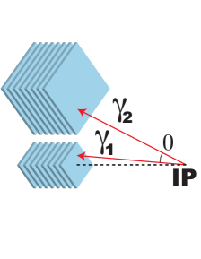
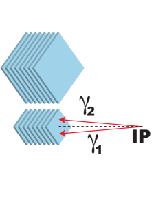
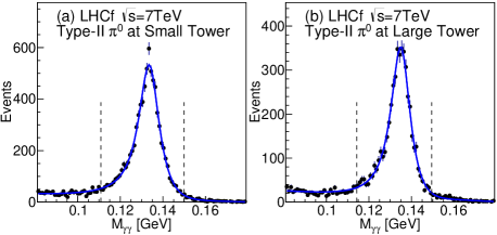
Figure 2 shows the reconstructed two-photon invariant mass ($M_{\gamma\gamma}$) distributions of LHCf data in the rapidity range $8.8<y<10.8$. The left and right panels of Fig. 2 show the distributions for Type-II events in the Arm2 small calorimeter and Arm2 large calorimeter respectively. The sharp peaks around $135\text{\,}\mathrm{MeV}$ are due to $\pi^{0}$ events. The distributions in Fig. 2 are based only on data from $p+p$ collisions at $\sqrt{s}=$7\text{\,}\mathrm{TeV}$$ during LHC Fill 1104. Similar invariant mass distributions are obtained from other fills and from Arm1. Kinematic quantities of the $\pi^{0}$s (four-momenta, $p_{\text{T}}$, $p_{\text{z}}$ and rapidity) are reconstructed by using the photon energies and incident positions measured by the LHCf calorimeters, and are used for producing the $p_{\text{T}}$ and $p_{\text{z}}$ distributions. The projected position of the proton beam axis on the LHCf detector (beam center) is used in order to derive the correct $p_{\text{T}}$ and $p_{\text{z}}$ values of each event. The beam center position is obtained from the LHCf position-sensitive detectors of Arm1 and Arm2 for each fill.

Figure 2: (color online). Reconstructed invariant mass distributions in $p+p$ collisions at $\sqrt{s}=$7\text{\,}\mathrm{TeV}$$. Left: Type-II $\pi^{0}$ events in the Arm2 small calorimeter. Right: Type-II $\pi^{0}$ events in the Arm2 large calorimeter. The solid curves show the best-fit composite physics model to the invariant mass distributions.

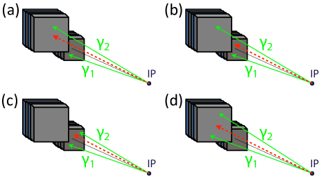
The $\pi^{0}$ event selection criteria that are applied prior to the reconstruction of the $\pi^{0}$ kinematics are summarized in Table. 1. Type-I events accompanied by at least one additional background particle in one of the two calorimeters (usually a photon or a neutron) and not originating in a $\pi^{0}$ decay are denoted as multi-hit $\pi^{0}$ events and are rejected as background events. Similarly, Type-II events accompanied by at least one additional background particle in the calorimeter used for $\pi^{0}$ identification are rejected. Figure 3 shows diagrams of all types of multi-hit events that are rejected. Panels (a) and (b) show the multi-hit Type-I $\pi^{0}$ events and panels (c) and (d) show the multi-hit Type-II $\pi^{0}$ events. Red and green arrows indicate a background particle not originating in a $\pi^{0}$ decay and two photons originating in a $\pi^{0}$ decay, respectively. The final inclusive production rates reported in this paper are corrected for these cut efficiencies and will be discussed in Sec. V.2.

Figure 3: (color online). Diagrams of all multi-hit events that are rejected. Panels (a) and (b) show the multi-hit Type-I $\pi^{0}$ events and panels (c) and (d) show the multi-hit Type-II $\pi^{0}$ events. Red and green arrows indicate a background particle not originating in a $\pi^{0}$ decay and two photons originating in a $\pi^{0}$ decay, respectively.

Table 1: Summary of criteria for selection of the $\pi^{0}$ sample.

Type-I $\pi^{0}$ events
Incident position	Within $2\text{\,}\mathrm{mm}$ from the edge of calorimeter
Energy threshold	$E_{\text{photon}}>$100\text{\,}\mathrm{GeV}$$
Number of hits	Single-hit in each calorimeter
PID	Photon-like in each calorimeter
Type-II $\pi^{0}$ events
Incident position	Within $2\text{\,}\mathrm{mm}$ from the edge of calorimeter
Energy threshold	$E_{\text{photon}}>$100\text{\,}\mathrm{GeV}$$
Number of hits	Two hits
PID	Photon-like

V.2 Corrections for experimental effects

The raw $p_{\text{T}}$ and $p_{\text{z}}$ distributions of $\pi^{0}$s are corrected for: (1) contamination by background events, (2) reconstruction inefficiency and the smearing caused by finite position and energy resolutions, (3) geometrical acceptance and the branching ratio of $\pi^{0}$ decay, and (4) the efficiency of the multi-hit $\pi^{0}$ cut. We now discuss each of these corrections in some detail.

V.2.1 Background contamination

First, the background contamination of the $\pi^{0}$ events from hadronic events, and from the coincidence of two photons not originating from the decay of a single $\pi^{0}$ are estimated using a sideband method LHCfpppi0 . As shown in Fig. 2 for instance, the reconstructed two-photon invariant mass distributions of LHCf data are fit to a composite physics model (solid blue curve). The model consists of an asymmetric Gaussian distribution for the $\pi^{0}$ signal component and a third order Chebyshev polynomial function for the background component. The fit is performed over the two photon invariant mass range $0.08<M_{\gamma\gamma}<$0.18\text{\,}\mathrm{GeV}$$. The $\pi^{0}$ signal window is defined by the two dashed vertical lines in Fig. 2 that are placed $\pm 3\sigma$ from the mean value. Here the mean value and the standard deviation are obtained from the best-fit asymmetric Gaussian distribution. The background window is defined as the region within $\pm 6\sigma$ distance from the peak value and excluding the $\pi^{0}$ signal window. The fraction of the background component included in the $\pi^{0}$ signal window can be estimated using the ratio of the integral of the best-fit third order Chebyshev function over the $\pi^{0}$ signal window divided by the integral over the $\pi^{0}$ signal and background windows. The width of the asymmetric Gaussian function comes from the detector response, predominantly from shower leakage near the edges of the calorimeters. The reconstructed energy is corrected for shower leakage.

V.2.2 Reconstruction inefficiency and smearing in position and energy resolution

Second, a spectrum unfolding is performed to simultaneously correct for both the reconstruction inefficiency and the smearing caused by finite position and energy resolution. The contamination by background events that has been estimated by the sideband method is taken into account in the unfolding process. We follow basically same unfolding procedure as in the previous analyses LHCfpppi0 ; LHCfpPbpi0 , although the unfolding algorithm is based on a fully Bayesian unfolding method Choudalakis instead of an iterative Bayesian unfolding method Dagostini . The calculation of the “a posteriori” probability in multi-dimensional space (the measured spectrum multiplied by the true spectrum) is achieved using a Markov Chain Monte Carlo simulation Caldwell . The convergence of the Markov Chain Monte Carlo simulation is ensured by the Gelman-Rubin test Gelman . Production of the MC events used for the calculation of the response matrix for the unfolding is explained in Sec. IV.1.

V.2.3 Geometric acceptance and branching ratio corrections

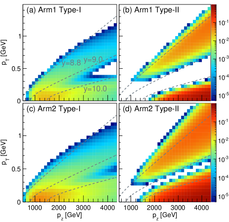
Thirdly, the limiting aperture of the LHCf calorimeters is estimated by using MC simulations. The procedure for performing MC simulations is given in Ref. LHCfpppi0 . Figure 4 shows the acceptance efficiency as a function of the $\pi^{0}$ $p_{\text{z}}$ and $p_{\text{T}}$. The acceptance efficiency has been obtained by taking the ratio of the $p_{\text{z}}$–$p_{\text{T}}$ distribution of $\pi^{0}$s that are within the aperture of the LHCf calorimeters divided by the distribution of all simulated $\pi^{0}$s. The fiducial cuts LHCfpppi0 and reconstructed energy cut (both of the $\pi^{0}$ decay photons must have $E>$100\text{\,}\mathrm{GeV}$$) are also applied to the accepted $\pi^{0}$ events. Dashed curves in Fig. 4 indicate lines of constant $\pi^{0}$ rapidity. The acceptance efficiencies in Fig. 4 are purely kinematic and do not depend upon a particular hadronic interaction model. The aperture correction is achieved by dividing, point by point, the distributions before the acceptance correction by the acceptance efficiency. The branching ratio inefficiency is due to $\pi^{0}$ decay into channels other than two photons. The branching ratio for $\pi^{0}$ decay into two photons is $98.8\text{\,}\mathrm{\char 37\relax}$ and is taken into account by increasing the $\pi^{0}$ acceptance efficiency by $1.2\text{\,}\mathrm{\char 37\relax}$.

V.2.4 Loss of events due to the multi-hit $\pi^{0}$ cut

Fourth, in order that the reported $\pi^{0}$ distributions represent inclusive cross sections it is necessary to correct the data for the loss of events due to the multi-hit cut (Sec. V.1.4). The correction factor is defined as $f^{\textrm{multihit}}_{i}=(N^{\textrm{multi}}_{i}+N^{\textrm{single}}_{i})/N^{\textrm{single}}_{i}$, where $N^{\textrm{multi}}_{i}$ and $N^{\textrm{single}}_{i}$ are the number of expected multihit and single-hit $\pi^{0}$ events in the $i$-th bin respectively. The factors $f^{\textrm{multihit}}_{i}$ are estimated using hadronic interaction models introduced in Sec. IV.1 and are in the range $1.0<f^{\textrm{multihit}}_{i}<1.1$ over all the $p_{\text{T}}$ and $p_{\text{z}}$ bins. LHCf $p_{\text{T}}$ and $p_{\text{z}}$ distributions are then multiplied by the average of these factors for the various interaction models and their contribution to the systematic uncertainty is derived from the observed variations amongst the interaction models. Consequently, the single-hit $\pi^{0}$ distributions are corrected to represent inclusive $\pi^{0}$ production distributions. All the procedures just described have been verified using the MC simulations introduced in Sec. IV.1.

Figure 4: (color online). The acceptance map of $\pi^{0}$ detection by the LHCf detectors in $p_{\text{z}}$–$p_{\text{T}}$ phase space: Arm1 Type-I (left top), Arm1 Type-II (right top), Arm2 Type-I (left bottom), and Arm2 Type-II (right bottom). The fiducial area cuts and energy threshold ($E_{\text{photon}}>$100\text{\,}\mathrm{GeV}$$) are taken into account. Dashed curves indicate lines of constant rapidity $\pi^{0}$s, $y$ = 8.8, 9.0, and 10.0 reading from top to bottom.

V.3 Systematic uncertainties

Systematic uncertainties are determined by three factors: (1) possible biases in event reconstruction, (2) uncertainty of the LHC machine conditions, and (3) an interaction model dependence.

V.3.1 Systematic uncertainties in event reconstructions and unfolding of distributions

Uncertainties related to biases in event reconstruction are mainly due to five causes: (1) single-hit/multi-hit separation, (2) PID, (3) energy scale uncertainty, (4) position-dependent corrections for both shower leakage and the light yield of the calorimeters, and (5) unfolding of distributions. For the first four terms, we follow the same approaches to estimate the systematic uncertainties as we used in the previous study LHCfpppi0 .

Concerning the unfolding process, the uncertainty is estimated by adding the following three components in quadrature. First, the uncertainty due to a possible dependence of the unfolding procedure on the shape of the $p_{\text{T}}$ or $p_{\text{z}}$ distributions to be unfolded is estimated from MC simulations; we estimate the variation of the ratios of the unfolded distributions to the true distributions among the three true distributions predictions by dpmjet, qgsjet, and epos. The second component is a dependence of the unfolding procedure on the event generator used in the generation of the response matrix for unfolding, which is negligible as we mentioned in Sec. IV.1. Finally, the third component is the systematic uncertainty in the unfolding algorithm itself. This is evaluated by comparing two unfolded distributions, one obtained by a fully Bayesian unfolding method and the second obtained by the iterative Bayesian unfolding method. The uncertainty in the first component is $10\text{\,}\mathrm{\char 37\relax}$ over the all $p_{\text{T}}$ and $p_{\text{z}}$ bins, and the uncertainties in the other two components make no significant contribution. Thus we assign $10\text{\,}\mathrm{\char 37\relax}$ for the systematic uncertainty in the unfolding of $p_{\text{T}}$ and $p_{\text{z}}$ distributions.

V.3.2 Systematic uncertainties in the LHC machine conditions

The LHC machine conditions introduce systematic uncertainties in beam position and luminosity. The beam position at the LHCf detectors varies from fill to fill owing to variations of the beam transverse position and the crossing angles at IP1. The beam center positions at the LHCf detectors obtained for LHC Fills 1089 to 1134 by the LHCf position-sensitive detectors and by the beam position monitors (BPMSW) installed $\pm$21\text{\,}\mathrm{m}$$ from IP1 BPM are consistent with each other within $\pm$$1\text{\,}\mathrm{mm}$. The systematic shifts to the $p_{\text{T}}$ and $p_{\text{z}}$ distributions are then evaluated by taking the ratios of distributions with the beam center displaced by $\pm$1\text{\,}\mathrm{mm}$$ to distributions with no displacement present. The evaluated systematic shifts to the $p_{\text{T}}$ and $p_{\text{z}}$ distributions are 5–$20\text{\,}\mathrm{\char 37\relax}$ depending on the $p_{\text{T}}$ and $p_{\text{z}}$ values.

The uncertainty in the luminosity depends on the collision configuration. For the data in $p+p$ collisions at $\sqrt{s}=$7\text{\,}\mathrm{TeV}$$, the luminosity value used for the analysis is derived from the counting rate of the Front Counters. Considering the uncertainties in both the calibration of the Front Counters $\pm$3.4\text{\,}\mathrm{\char 37\relax}$$ and in the beam intensity measurement $\pm$5.0\text{\,}\mathrm{\char 37\relax}$$ during the Van der Meer scans, we estimate an uncertainty of $\pm$6.1\text{\,}\mathrm{\char 37\relax}$$ in the luminosity for $p+p$ collisions at $\sqrt{s}=$7\text{\,}\mathrm{TeV}$$ LHCfLumi . For the $p+p$ collision data at $\sqrt{s}=$2.76\text{\,}\mathrm{TeV}$$ and $p+\text{Pb}$ collision data at $\sqrt{s_{\textrm{NN}}}=$5.02\text{\,}\mathrm{TeV}$$, LHCf data were taken simultaneously with data taken by the ATLAS experiment. The luminosity values used for this data analysis were then provided by the LHCf Front Counters and also by the ATLAS collaboration.

The luminosity uncertainties in $p+p$ collisions at $\sqrt{s}=$2.76\text{\,}\mathrm{TeV}$$ and in $p+\text{Pb}$ collisions at $\sqrt{s_{\textrm{NN}}}=$5.02\text{\,}\mathrm{TeV}$$ are estimated to be $\pm$3.1\text{\,}\mathrm{\char 37\relax}$$ ATLASPbPb and $\pm$20\text{\,}\mathrm{\char 37\relax}$$ CERNLumi , respectively.

Pileup of successive $p+\text{Pb}$ collisions due to the small bunch spacing ($200\text{\,}\mathrm{ns}$) relative to the data acquisition time ($500\text{\,}\mathrm{ns}$) amounts to $<$5\text{\,}\mathrm{\char 37\relax}$$ systematic uncertainty of $p_{\text{T}}$ and $p_{\text{z}}$ distributions (see Sec. III.2), and may provide a slight shift of the absolute normalization for the $p_{\text{T}}$ and $p_{\text{z}}$ distributions. This effect is not corrected for in this study, but is taken into account as uncertainty related to the LHC machine condition.

V.3.3 Systematic uncertainties depending on the interaction models used in the MC simulations

The analysis in this paper unavoidably relies on the predictions given by MC simulations. First, we correct LHCf data for the loss of multi-hit $\pi^{0}$ events (Sec. V.2.4). The correction factors $f^{\textrm{multihit}}$ show a systematic uncertainty of less than $10\text{\,}\mathrm{\char 37\relax}$ among the hadronic interaction models. Second, for $p+\text{Pb}$ collisions only, the contamination from UPC induced $\pi^{0}$ events in LHCf data is derived from MC simulations (Sec. IV.1). The comparison of the predicted $p_{\text{T}}$ and $p_{\text{z}}$ distributions of $\pi^{0}$s between two UPC MC simulations, one using dpmjet 3.05 and the other one using pythia 6.428 for high-energy photon–proton interaction, show a systematic uncertainty of roughly 3–$20\text{\,}\mathrm{\char 37\relax}$.

In summary, there are 10 systematic uncertainties. The first four (1) Single/multihit selection, (2) PID, (3) energy scale and (4) position-dependent correction are explained in Ref. LHCfpppi0 and we follow the same approaches as we used in Ref. LHCfpppi0 . The remaining six systematic uncertainties and the text containing their explanations are: (5) Unfolding uncertainty is explained and evaluated in Sec. V.3.1, (6) Offset of beam axis is explained in the 1st paragraph of Sec. V.3.2, 5–$20\text{\,}\mathrm{\char 37\relax}$ shifts in $p_{\text{T}}$ or $p_{\text{z}}$ distributions are obtained, (7) Luminosity uncertainty is explained in the 2nd paragraph of Sec. V.3.2. (8) Contamination of successive $p+\text{Pb}$ collisions is explained in the 3rd paragraph of Sec. V.3.2, (This uncertainty is due to contamination and thus only a positive error is quoted.) (9) The uncertainty in multihit $\pi^{0}$ events $\pm$10\text{\,}\mathrm{\char 37\relax}$$, and (10) the uncertainty in UPC $\pm$(3–$20\text{\,}\mathrm{\char 37\relax}$) are found in Sec. V.3.3. Table 2 summarizes the systematic uncertainties of the $\pi^{0}$ $p_{\text{T}}$ and $p_{\text{z}}$ distributions.

Table 2: Summary of the systematic uncertainties. Numerical values indicate the maximum variation of bin contents in the $p_{\text{T}}$ and $p_{\text{z}}$ distributions due to systematic uncertainties. Note that the uncertainty in contamination of successive $p+\text{Pb}$ collisions and in UPC $\pi^{0}$ simulation pertain only to $p+\text{Pb}$ collisions.

Single/multihit selection	$\pm$$3\text{\,}\mathrm{\char 37\relax}$
Particle identification	$\pm$(0–$20\text{\,}\mathrm{\char 37\relax}$)
Energy scale	$\pm$(5–$20\text{\,}\mathrm{\char 37\relax}$)
Position-dependent correction	$\pm$(5–$30\text{\,}\mathrm{\char 37\relax}$)
Unfolding	$\pm$(5–$10\text{\,}\mathrm{\char 37\relax}$)
Offset of beam axis	$\pm$(5–$20\text{\,}\mathrm{\char 37\relax}$)
Luminosity ($p+p$ at $7\text{\,}\mathrm{TeV}$)	$\pm$$6.1\text{\,}\mathrm{\char 37\relax}$
Luminosity ($p+p$ at $2.76\text{\,}\mathrm{TeV}$)	$\pm$$3.1\text{\,}\mathrm{\char 37\relax}$
Luminosity ($p+\text{Pb}$ at $5.02\text{\,}\mathrm{TeV}$)	$\pm$$20\text{\,}\mathrm{\char 37\relax}$
Contamination of successive $p+\text{Pb}$ collisions	<$5\text{\,}\mathrm{\char 37\relax}$
Multihit $\pi^{0}$ correction	<$10\text{\,}\mathrm{\char 37\relax}$
UPC $\pi^{0}$ simulation	$\pm$(3–$20\text{\,}\mathrm{\char 37\relax}$)

VI Analysis results

VI.1 Results in $p+p$ collisions at $\sqrt{s}=$7\text{\,}\mathrm{TeV}$$

The inclusive production rate of neutral pions as a function of $p_{\text{T}}$ and $p_{\text{z}}$ is given by the expression PDG

$$\frac{1}{\sigma_{\text{inel}}}E\frac{d^{3}\sigma}{dp^{3}}\Rightarrow\frac{1}{N_{\text{inel}}}\frac{d^{2}N(p_{\text{T}},y)}{2\pi p_{\text{T}}dp_{\text{T}}dy}=\frac{1}{N_{\text{inel}}}E\frac{d^{2}N(p_{\text{T}},p_{\text{z}})}{2\pi p_{\text{T}}dp_{\text{T}}dp_{\text{z}}}.$$ (1)

$\sigma_{\text{inel}}$ is the inelastic cross section for $p+p$ collisions at $\sqrt{s}=$7\text{\,}\mathrm{TeV}$$. $Ed^{3}\sigma/dp^{3}$ is the inclusive cross section for $\pi^{0}$ production. The number of inelastic collisions, $N_{\text{inel}}$, used for the production rate normalization is calculated from $N_{\text{inel}}$ = $\sigma_{\text{inel}}\int{\cal L}dt$, taking the inelastic cross section $\sigma_{\text{inel}}=$73.6\text{\,}\mathrm{mb}$$ LHCfpppi0 . The uncertainty in $\sigma_{\text{inel}}$ is estimated to be $\pm$3.0\text{\,}\mathrm{mb}$$ by comparing the values of $\sigma_{\text{inel}}$ reported in Refs. TOTEMinel1 ; TOTEMinel2 ; TOTEMinel3 ; ATLASinel .

Using the integrated luminosities $\int{\cal L}dt$, reported in Sec. III.1, $N_{\text{inel}}$ is $(2.67\pm 0.11)\text{\times}{10}^{8}$ for Arm1 and $(2.10\pm 0.09)\text{\times}{10}^{8}$ for Arm2. $d^{2}N(p_{\text{T}},y)$ is the number of $\pi^{0}$s produced within the transverse momentum interval $dp_{\text{T}}$ and the rapidity interval $dy$. Similarly $d^{2}N(p_{\text{T}},p_{\text{z}})$ is the number of $\pi^{0}$s produced within $dp_{\text{T}}$ and the longitudinal momentum interval $dp_{\text{z}}$.

Experimental $p_{\text{T}}$ and $p_{\text{z}}$ distributions measured independently with the Arm1 and Arm2 detectors are combined following a pull method Pull and the final $p_{\text{T}}$ and $p_{\text{z}}$ distributions are then obtained by minimizing the value of the chi-square function defined by

$$\chi^{2}=\sum_{i=1}^{n}\sum_{a=1}^{5}\left(\frac{R_{a,i}^{\text{obs}}(1+\mathit{S}_{a,i})-R_{i}^{\text{comb}}}{\sigma_{a,i}}\right)^{2}+\chi^{2}_{\text{penalty}},$$ (2)

where the index $i$ represents the $p_{\text{T}}$ or $p_{\text{z}}$ bin number running from 1 to $n$ (the total number of $p_{\text{T}}$ or $p_{\text{z}}$ bins), and the index $a$ indicates the type of distributions: $a=1$ Arm1 Type-I events, $a=2$ Arm1 Type-II events with the Large Calorimeter, $a=3$ Arm2 Type-I events, $a=4$ Arm2 Type-II events with the Small Calorimeter, and $a=5$ Arm2 Type-II events with the Large Calorimeter. Note that Arm1 Type-II events with the Small Calorimeter are not used for this analysis since the energy reconstruction accuracy for these events is still being investigated. $R_{a,i}^{\text{obs}}$ is the inclusive production rate in the $i$th bin of the $a$th distribution, which corresponds to the second and third terms Eq. (1). $R_{i}^{\text{comb}}$ is the inclusive production rate in the $i$th bin obtained by combining all $R_{a,i}^{\text{obs}}$’s for $a=$1–5. $\sigma_{a,i}$ is the uncertainty of $R_{a,i}^{\text{obs}}$. The $\sigma_{a,i}$ are calculated by quadratically adding the statistical uncertainty and the systematic uncertainty in the energy scale. The energy scale uncertainty has been estimated with test beam data taken at the SPS and is uncorrelated bin-by-bin unlike the other systematic uncertainties LHCfpppi0 . The systematic correction $\mathit{S}_{a,i}$ modifies the number of events in the $i$th bin of the $a$th distribution:

$$\mathit{S}_{a,i}=\sum_{j=1}^{7}f_{a,i}^{j}\varepsilon_{a}^{j}.$$ (3)

The coefficient $f_{a,i}^{j}$ is the systematic shift of the $i$th bin content of the $a$th distribution due to the $j$th systematic uncertainty term. The systematic uncertainty consists of seven uncertainties related to the single-hit/multihit separation, the PID, the energy scale (owing to the invariant mass shift of the measured $\pi^{0}$ events), the position-dependent correction, the unfolding procedure, the beam center position, and the loss of multihit $\pi^{0}$ events. These uncertainties are assumed to be fully uncorrelated between the Arm1 and Arm2 detectors, while correlations between Type-I and Type-II events and bin-bin correlations have been accounted for. The coefficients $\varepsilon_{a}^{j}$, which should follow a Gaussian distribution, can be varied, within the constraints of the penalty term given by

$$\chi^{2}_{\text{penalty}}=\sum_{j=1}^{7}\sum_{a=1}^{5}|\varepsilon_{a}^{j}|^{2},$$ (4)

to achieve the minimum $\chi^{2}$ value for each chi-square test. Note that the uncertainty in the luminosity determination, $\pm$3.1\text{\,}\mathrm{\char 37\relax}$$–$\pm$20\text{\,}\mathrm{\char 37\relax}$$, not included in Eq. (3) and Eq. (4), can cause independent shifts of all the $p_{\text{T}}$ and $p_{\text{z}}$ distributions.

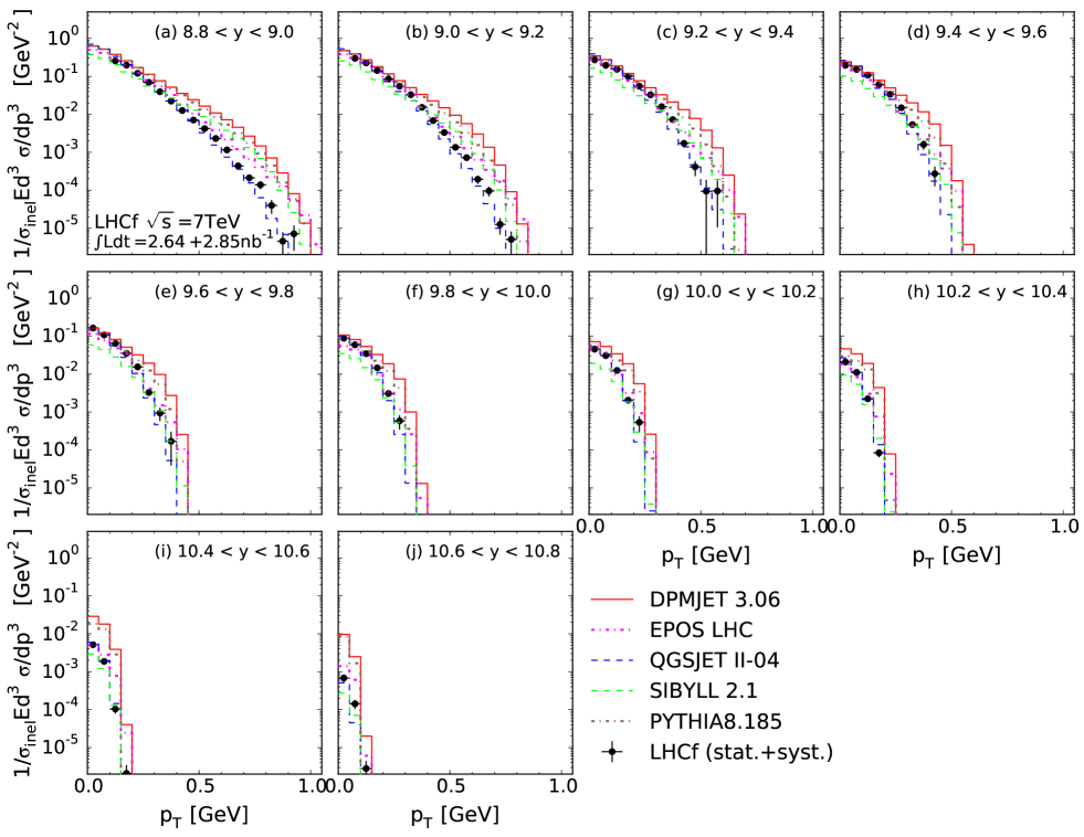
The LHCf $p_{\text{T}}$ distributions (filled circles) are obtained from the best-fit $R^{\text{comb}}$ and are shown in Fig. 5. The $68\text{\,}\mathrm{\char 37\relax}$ confidence intervals incorporating the statistical and systematic uncertainties, except for the luminosity uncertainty, are indicated by the error bars. LHCf $p_{\text{T}}$ distributions are corrected for the influences of the detector response, event selection efficiencies and geometrical acceptance efficiencies, and thus LHCf $p_{\text{T}}$ distributions can be compared directly to the predicted $p_{\text{T}}$ distributions from hadronic interaction models. For comparison, the predictions from various hadronic interaction models are also shown in Fig. 5: dpmjet (solid red line), qgsjet (dashed blue line), sibyll (dotted green line), epos (dashed-dotted magenta line), and pythia (default parameter set, dashed-double-dotted brown line). For these hadronic interaction models, the inelastic cross section used for the production rate normalization is taken from the predefined value in each model.

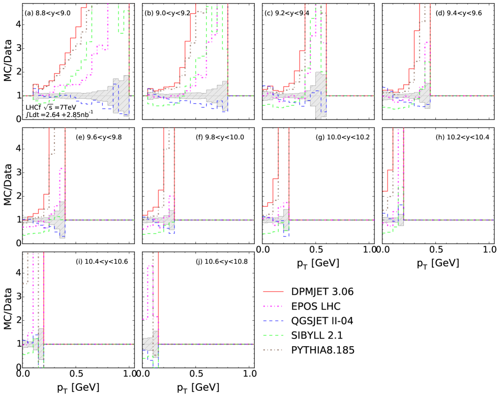
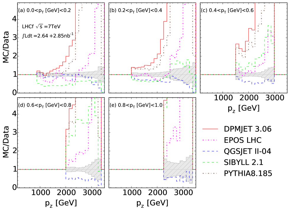
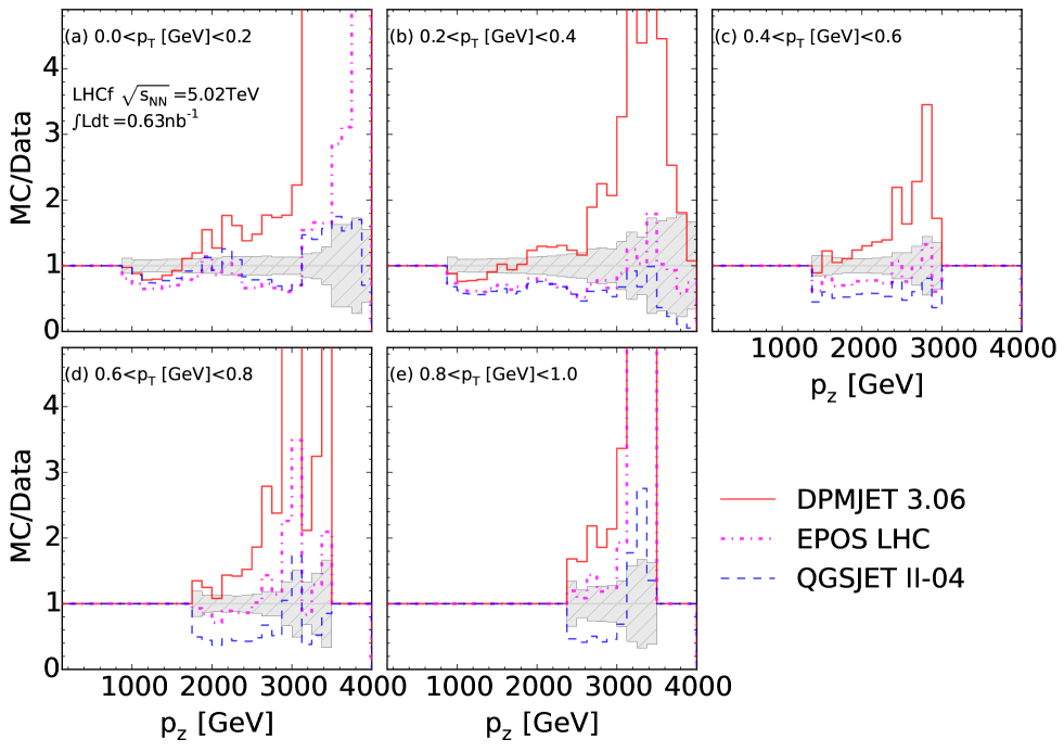
Figure 6 presents the ratios of the inclusive production rates predicted by the hadronic interaction models listed above to those obtained by LHCf data. Shaded areas have been taken from the statistical and systematic uncertainties. In Fig. 6, the denominator and the numerators, namely the inclusive production rate for LHCf data and for the hadronic interaction models, respectively, are properly normalized by the inelastic cross section for each, thus we do not apply any other normalization to the ratios. The inclusive production rates of $\pi^{0}$s measured by LHCf and the ratios of $\pi^{0}$ production rate of MC simulation to data are summarized in Appendix.

In the comparisons in Fig. 5 and 6, qgsjet has good overall agreement with LHCf data, while epos produces a slightly harder distribution than the LHCf data for $p_{\text{T}}>$0.5\text{\,}\mathrm{GeV}$$. These two models are based on the parton-based Gribov-Regge approach Gribov1 ; Regge and are tuned by using the present LHC data (ALICE, ATLAS, CMS, and TOTEM) QGSJET ; EPOS . The prediction of sibyll agrees well with the LHCf data for $8.8<y<9.2$ and $p_{\text{T}}<$0.4\text{\,}\mathrm{GeV}$$, while the absolute yield of sibyll is about half that of the LHCf data for $y>9.2$. The predictions of dpmjet and pythia are compatible with LHCf data for $9.0<y<9.8$ and $p_{\text{T}}<$0.2\text{\,}\mathrm{GeV}$$, while for $p_{\text{T}}>$0.2\text{\,}\mathrm{GeV}$$ they become significantly harder than both LHCf data and the other model predictions. Generally the harder distributions appearing in sibyll, dpmjet, and pythia can be attributed to the baryon/meson production mechanism that is used by these models. For example the popcorn approach Andersson ; Eden implemented in the Lund model is known to produce hard distributions of forward mesons Drescher2 . Indeed, by only changing the tuning parameters of the popcorn approach in dpmjet one obtains softer meson distributions and consequently $p_{\text{T}}$ distributions that are compatible with LHCf data. However such a crude tune may bring disagreements between the model predictions and other experimental results, e.g. forward neutron $p_{\text{z}}$ and $p_{\text{T}}$ distributions.

Figure 5: (color online). LHCf $p_{\text{T}}$ distributions (filled circles) in $p+p$ collisions at $\sqrt{s}=$7\text{\,}\mathrm{TeV}$$. Error bars indicate the total statistical and systematic uncertainties. The predictions of hadronic interaction models are shown for comparison: dpmjet (solid red line), qgsjet (dashed blue line), sibyll (dotted green line), epos (dashed-dotted magenta line), and pythia (dashed-double-dotted brown line).

Figure 6: (color online). Ratios of LHCf $p_{\text{T}}$ distributions to the $p_{\text{T}}$ distributions predicted by hadronic interaction models in $p+p$ collisions at $\sqrt{s}=$7\text{\,}\mathrm{TeV}$$ are shown by solid red line (dpmjet), dashed blue line (qgsjet), dotted green line (sibyll), dashed-dotted magenta line (epos), and dashed-double-dotted brown line (pythia). Shaded areas indicate the range of total uncertainties of the LHCf $p_{\text{T}}$ distributions.

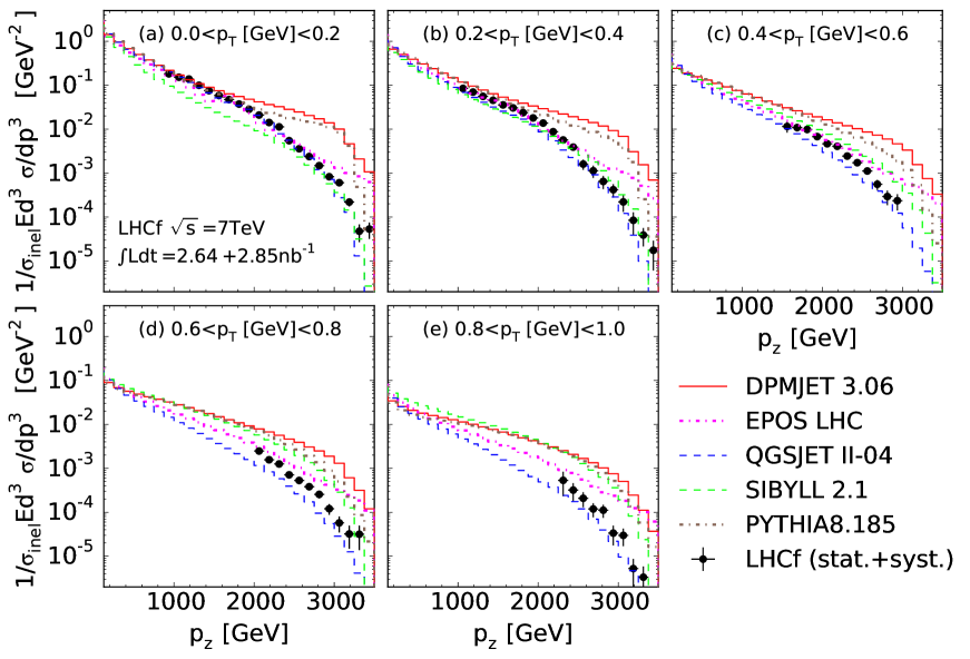
The LHCf $p_{\text{z}}$ distributions are shown in Fig. 7. The $p_{\text{z}}$ distributions predicted by various hadronic interaction models are also shown in Fig. 7. Figure 8 presents the ratios of $p_{\text{z}}$ distributions predicted by the hadronic interaction models to the LHCf $p_{\text{z}}$ distributions. Shaded areas have been taken from the statistical and systematic uncertainties. The same conclusions for the comparisons are obtained as those found for Fig. 5 and 6. There is again an overall agreement between LHCf data and the qgsjet prediction, especially for $0.0<p_{\text{T}}<$0.2\text{\,}\mathrm{GeV}$$. The epos prediction is compatible with LHCf data for $p_{\text{T}}<$2\text{\,}\mathrm{TeV}$$, while showing a hard slope for $p_{\text{T}}>$2\text{\,}\mathrm{TeV}$$ in all $p_{\text{T}}$ regions. The predictions by dpmjet and pythia agree with LHCf data for $p_{\text{T}}<$0.2\text{\,}\mathrm{GeV}$$ and $p_{\text{z}}<$1.6\text{\,}\mathrm{TeV}$$, while showing a harder distribution for the higher $p_{\text{z}}$ regions. sibyll predicts a smaller production of $\pi^{0}$s for $p_{\text{T}}<$0.2\text{\,}\mathrm{GeV}$$ and becomes similar with dpmjet and pythia with increasing $p_{\text{T}}$.

Figure 7: (color online). LHCf $p_{\text{z}}$ distributions (filled circles) in $p+p$ collisions at $\sqrt{s}=$7\text{\,}\mathrm{TeV}$$. Error bars indicate the total statistical and systematic uncertainties. The predictions of hadronic interaction models are shown for comparison: dpmjet (solid red line), qgsjet (dashed blue line), sibyll (dotted green line), epos (dashed-dotted magenta line), and pythia (dashed-double-dotted brown line).

Figure 8: (color online). Ratios of LHCf $p_{\text{z}}$ distributions to the $p_{\text{z}}$ distributions predicted by hadronic interaction models in $p+p$ collisions at $\sqrt{s}=$7\text{\,}\mathrm{TeV}$$ are shown by solid red line (dpmjet), dashed blue line (qgsjet), dotted green line (sibyll), dashed-dotted magenta line (epos), and dashed-double-dotted brown line (pythia). Shaded areas indicate the range of total uncertainties of the LHCf $p_{\text{z}}$ distributions.

VI.2 Results in $p+p$ collisions at $\sqrt{s}=$2.76\text{\,}\mathrm{TeV}$$

The inclusive production rates of $\pi^{0}$s as a function of $p_{\text{T}}$ and $p_{\text{z}}$ are given by Eq. (1). Using the inelastic cross section $\sigma_{\text{inel}}=$62.5\pm 5.0\text{\,}\mathrm{mb}$$ PDG and the integrated luminosities reported in Sec. III.3, $N_{\text{inel}}$ is calculated as $(1.60\pm 0.13)\text{\times}{10}^{8}$. The uncertainty on $\sigma_{\text{inel}}$ is estimated by comparing the $\sigma_{\text{inel}}$ value with the present experimental result ALICEinel . Note that only the LHCf Arm2 detector was operated in $p+p$ collisions at $\sqrt{s}=$2.76\text{\,}\mathrm{TeV}$$ and that only Type-I events are used for the analysis since Type-II event kinematics are outside the calorimeter acceptance for $\sqrt{s}=$2.76\text{\,}\mathrm{TeV}$$.

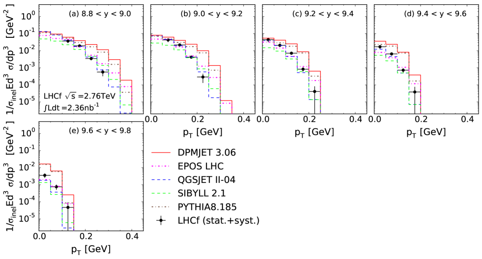
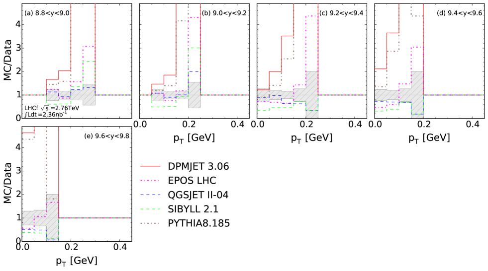
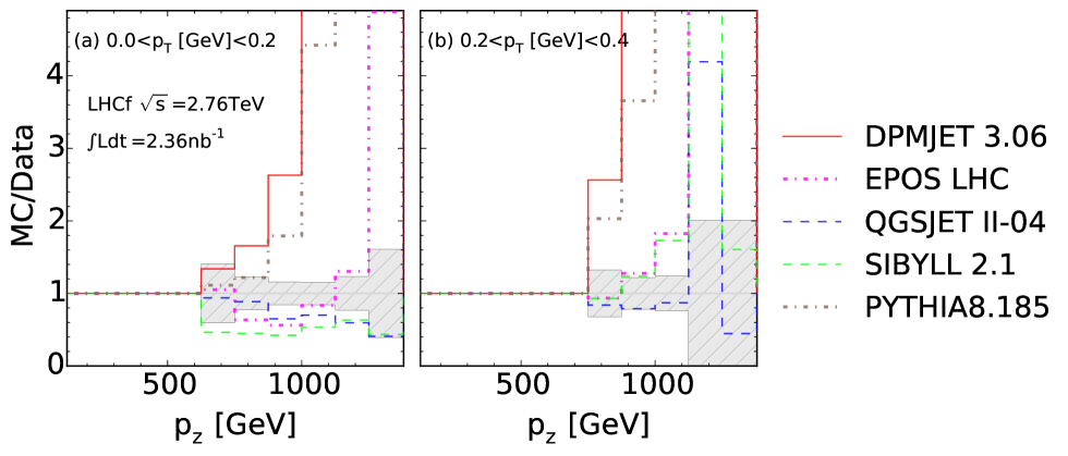
LHCf $p_{\text{T}}$ distributions are shown in Fig. 9. The $p_{\text{T}}$ distributions predictions for the hadronic interaction models are also shown in Fig. 9 for comparison. Figure 10 presents the ratios of $p_{\text{T}}$ distributions predicted by the hadronic interaction models to the LHCf $p_{\text{T}}$ distributions. qgsjet provides the best agreement with LHCf data, although it is slightly softer than the LHCf data for $y>9.2$. The prediction of epos shows a harder behavior than both qgsjet and LHCf data. sibyll tends to have generally a smaller $\pi^{0}$ yield and a harder distribution compared to qgsjet and epos, leading to the smaller and larger yields with respect to LHCf data in the $p_{\text{T}}$ regions below and above $0.1\text{\,}\mathrm{GeV}$. dpmjet and pythia predict larger $\pi^{0}$ yields than both LHCf data and other models over the entire rapidity range. The same discussion on the popcorn model in the previous Section VI.1 can be applied to the predictions of sibyll, dpmjet, and pythia.

Figure 9: (color online). LHCf $p_{\text{T}}$ distributions (filled circles) in $p+p$ collisions at $\sqrt{s}=$2.76\text{\,}\mathrm{TeV}$$. Error bars indicate the total statistical and systematic uncertainties. The predictions of hadronic interaction models are shown for comparison: dpmjet (solid red line), qgsjet (dashed blue line), sibyll (dotted green line), epos (dashed-dotted magenta line), and pythia (dashed-double-dotted brown line).

Figure 10: (color online). Ratios of LHCf $p_{\text{T}}$ distributions to the $p_{\text{T}}$ distributions predicted by hadronic interaction models in $p+p$ collisions at $\sqrt{s}=$2.76\text{\,}\mathrm{TeV}$$ are shown by solid red line (dpmjet), dashed blue line (qgsjet), dotted green line (sibyll), dashed-dotted magenta line (epos), and dashed-double-dotted brown line (pythia). Shaded areas indicate the range of total uncertainties of the $p_{\text{T}}$ spectra.

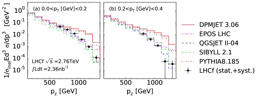
LHCf $p_{\text{z}}$ distributions are shown in Fig. 11. Figure 12 presents the ratios of $p_{\text{z}}$ distributions predicted by the hadronic interaction models to LHCf $p_{\text{z}}$ distributions. The same tendencies found in Fig. 7 are present here also qgsjet gives the best agreement for $0.0<p_{\text{T}}<$0.4\text{\,}\mathrm{GeV}$$ and epos has a harder behavior especially for $0.2<p_{\text{T}}<$0.4\text{\,}\mathrm{GeV}$$. The predictions of dpmjet and pythia are significantly harder than LHCf data for $p_{\text{T}}<$0.4\text{\,}\mathrm{GeV}$$ and show poor overall agreement with LHCf data. This can be explained by the popcorn model in a way similar to the harder $p_{\text{T}}$ distributions of the sibyll, dpmjet and pythia models found in Fig. 7 and the preceding Section.

Figure 11: (color online). LHCf $p_{\text{z}}$ distributions (filled circles) in $p+p$ collisions at $\sqrt{s}=$2.76\text{\,}\mathrm{TeV}$$. Error bars indicate the total statistical and systematic uncertainties. The predictions of hadronic interaction models are shown for comparison: dpmjet (solid red line), qgsjet (dashed blue line), sibyll (dotted green line), epos (dashed-dotted magenta line), and pythia (dashed-double-dotted brown line).

Figure 12: (color online). Ratios of LHCf $p_{\text{z}}$ distributions to the $p_{\text{z}}$ distributions predicted by hadronic interaction models in $p+p$ collisions at $\sqrt{s}=$2.76\text{\,}\mathrm{TeV}$$ are shown by solid red line (dpmjet), dashed blue line (qgsjet), dotted green line (sibyll), dashed-dotted magenta line (epos), and dashed-double-dotted brown line (pythia). Shaded areas indicate the range of total uncertainties of the $p_{\text{z}}$ distributions.

VI.3 Results in $p+\text{Pb}$ collisions at $\sqrt{s_{\textrm{NN}}}=$5.02\text{\,}\mathrm{TeV}$$

The inclusive $\pi^{0}$ production rate in $p+\text{Pb}$ collisions is given as

$$\frac{1}{\sigma^{\text{pPb}}_{\text{inel}}}E\frac{d^{3}\sigma^{\text{pPb}}}{dp^{3}} = \frac{1}{N^{\text{pPb}}_{\text{inel}}}\frac{d^{2}N^{\text{pPb}}(p_{\text{T}},y_{\text{lab}})}{2\pi p_{\text{T}}dp_{\text{T}}dy_{\text{lab}}}$$ (5)

$$= \frac{1}{N^{\text{pPb}}_{\text{inel}}}E\frac{d^{2}N^{\text{pPb}}(p_{\text{T}},p_{\text{z}})}{2\pi p_{\text{T}}dp_{\text{T}}dp_{\text{z}}},$$

where $\sigma^{\text{pPb}}_{\text{inel}}$ is the inelastic cross section, $Ed^{3}\sigma^{\text{pPb}}/dp^{3}$ is the inclusive cross section of $\pi^{0}$ production in $p+\text{Pb}$ collisions at $\sqrt{s_{\textrm{NN}}}=$5.02\text{\,}\mathrm{TeV}$$, and $y_{\text{lab}}$ is the rapidity in the detector reference frame. The number of inelastic $p+\text{Pb}$ collisions, $N^{\text{pPb}}_{\text{inel}}$, used for normalizing the production rates is calculated from $N^{\text{pPb}}_{\text{inel}}$ = $\sigma^{\text{pPb}}_{\text{inel}}\int{\cal L}dt$, assuming the inelastic $p+\text{Pb}$ cross section $\sigma^{\text{pPb}}_{\text{inel}}=$2.11\pm 0.11\text{\,}\mathrm{b}$$ dEnterria . The value for $\sigma^{\text{pPb}}_{\text{inel}}$ is derived from the inelastic $p+p$ cross section $\sigma^{\text{pp}}_{\text{inel}}$ and the Glauber multiple collision model dEnterria ; Glauber . The uncertainty on $\sigma^{\text{pPb}}_{\text{inel}}$ is estimated by comparing the $\sigma^{\text{pPb}}_{\text{inel}}$ value with other calculations and experimental results presented in Refs. ALICEpPb ; CMSpPb . Using the integrated luminosities described in Sec. III, $N^{\text{pPb}}_{\text{inel}}$ is $(9.33\pm 0.47)\text{\times}{10}^{7}$. Note that only the LHCf Arm2 detector (proton remnant side) was operated in $p+\text{Pb}$ collisions at $\sqrt{s_{\textrm{NN}}}=$5.02\text{\,}\mathrm{TeV}$$.

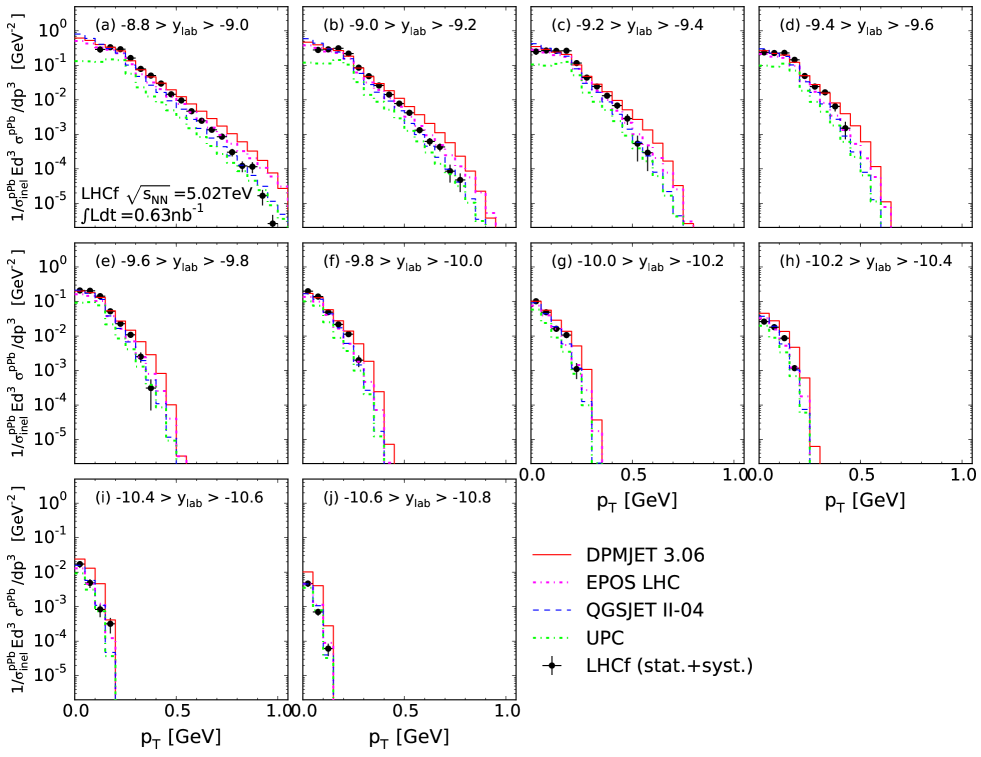
Figure 13 shows LHCf $p_{\text{T}}$ distributions with both statistical and systematic errors (filled circles and error bars). The $p_{\text{T}}$ distributions in $p+\text{Pb}$ collisions at $\sqrt{s_{\textrm{NN}}}=$5.02\text{\,}\mathrm{TeV}$$ predicted by the hadronic interaction models, dpmjet (solid red line), qgsjet (dashed blue line), and epos (dotted magenta line), are also shown in the same figure for comparison. The expected UPC contribution discussed in Sec. IV.1 is added to the hadronic interaction model predictions for consistency with the treatment of LHCf data, and the UPC $p_{\text{T}}$ distribution is shown for reference (dashed-double-dotted green line).

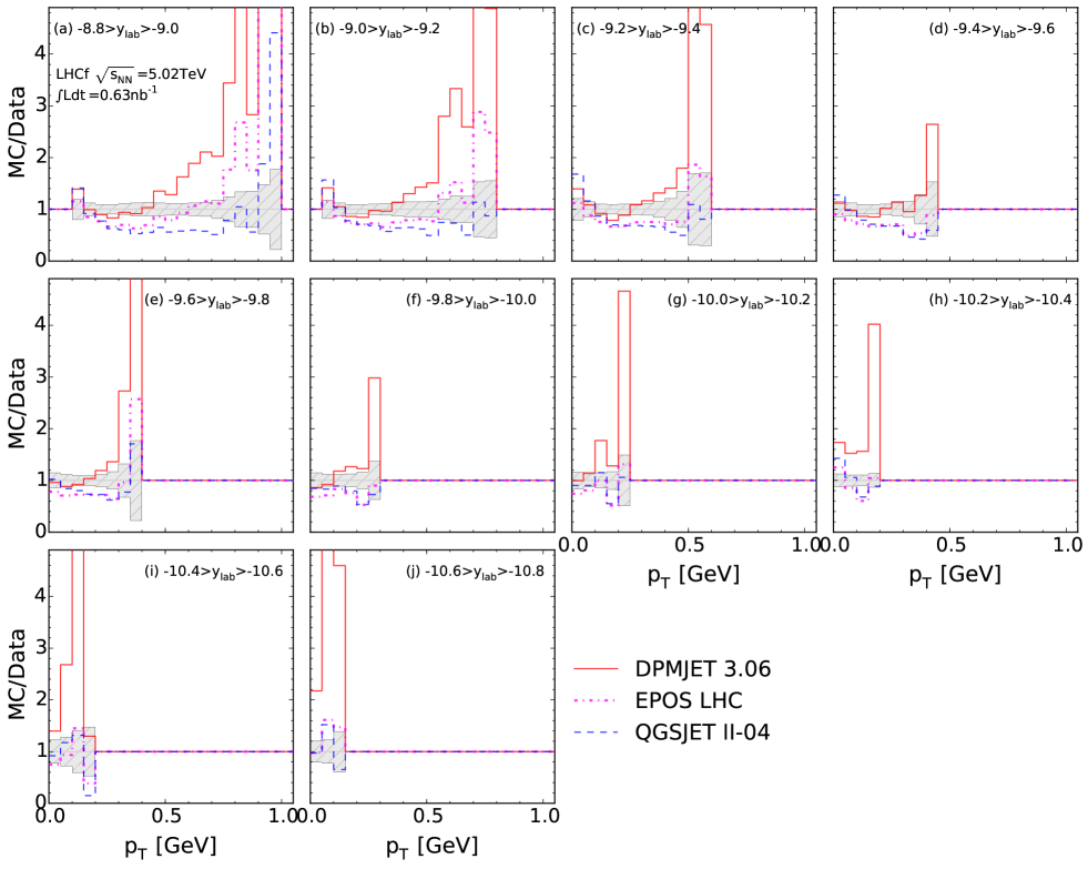
In Fig. 13, dpmjet shows good agreement with LHCf data at $-8.8>y_{\text{lab}}>-10.0$ and $p_{\text{T}}<$0.3\text{\,}\mathrm{GeV}$$, while showing a harder behavior at $-8.8>y_{\text{lab}}>-9.2$ and $p_{\text{T}}>$0.5\text{\,}\mathrm{GeV}$$. qgsjet and epos predict relatively similar distributions to each other and show better agreement with LHCf data for $p_{\text{T}}>$0.4\text{\,}\mathrm{GeV}$$ than dpmjet. The characteristic bump at $y_{\text{lab}}>-9.8$ and $0.1\lesssim p_{\text{T}}\lesssim$0.2\text{\,}\mathrm{GeV}$$, which is absent in $p+p$ collisions, originates from the channel $\gamma+p\to\pi^{0}+p$ via baryon resonances in UPCs. In fact the UPC simulation reproduces such a bump. Figure 14 presents the ratios of LHCf $p_{\text{T}}$ distributions to the $p_{\text{T}}$ distributions predicted by hadronic interaction models taking the UPC contribution into account in the $p_{\text{T}}$ distributions.

Figure 13: (color online). LHCf $p_{\text{T}}$ distributions (filled circles) in $p+\text{Pb}$ collisions at $\sqrt{s_{\textrm{NN}}}=$5.02\text{\,}\mathrm{TeV}$$. Error bars indicate the total statistical and systematic uncertainties. The predictions of hadronic interaction models are shown for comparison: dpmjet (solid red line), qgsjet (dashed blue line), and epos (dashed-dotted magenta line).

Figure 14: (color online). Ratios of LHCf $p_{\text{T}}$ distributions to the $p_{\text{T}}$ distributions predicted by hadronic interaction models in $p+\text{Pb}$ collisions at $\sqrt{s_{\textrm{NN}}}=$5.02\text{\,}\mathrm{TeV}$$ are shown by solid red line (dpmjet), dashed blue line (qgsjet), and dashed-dotted magenta line (epos). Shaded areas indicate the range of total uncertainties of the $p_{\text{T}}$ distributions.

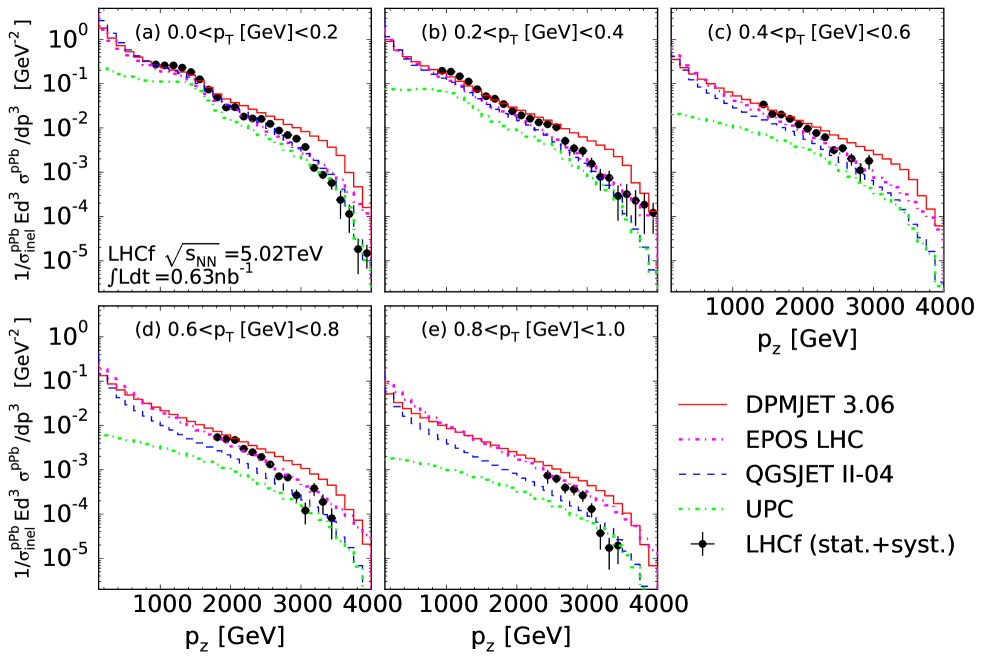
The $p_{\text{z}}$ distributions are shown in Fig. 15. Figure 16 presents the ratios of LHCf $p_{\text{z}}$ distributions to the $p_{\text{z}}$ distributions predicted by the hadronic interaction models. A similar tendency to that found in $p+p$ collisions at $\sqrt{s}=$7\text{\,}\mathrm{TeV}$$ is found for LHCf data relative to model predictions. Concerning the comparison of hadronic interaction models with LHCf data, qgsjet shows a very good agreement at $p_{\text{T}}<$0.2\text{\,}\mathrm{GeV}$$. However at $p_{\text{T}}>$0.2\text{\,}\mathrm{GeV}$$, there are no models giving a consistent description of LHCf data within uncertainty over all $p_{\text{z}}$ bins, although epos shows a certain compatibility with LHCf data for $p_{\text{T}}>$0.4\text{\,}\mathrm{GeV}$$ and for $p_{\text{z}}<$3\text{\,}\mathrm{TeV}$$. The dpmjet predictions agree with LHCf data at $p_{\text{T}}<$0.6\text{\,}\mathrm{GeV}$$ and $p_{\text{z}}<$2\text{\,}\mathrm{TeV}$$, while showing a harder distribution at higher $p_{\text{z}}$ similar to $p+p$ collisions. Again note the characteristic bump found in the LHCf data at $p_{\text{z}}\sim$1.2\text{\,}\mathrm{TeV}$$ and $p_{\text{T}}<$0.4\text{\,}\mathrm{GeV}$$, originating from the channel $\gamma+p\to\pi^{0}+p$ via baryon resonances in UPCs.

Figure 15: (color online). LHCf $p_{\text{z}}$ distributions (filled circles) in $p+\text{Pb}$ collisions at $\sqrt{s_{\textrm{NN}}}=$5.02\text{\,}\mathrm{TeV}$$. Error bars indicate the total statistical and systematic uncertainties. The predictions of hadronic interaction models are shown for comparison: dpmjet (solid red line), qgsjet (dashed blue line), and epos (dashed-dotted magenta line).

Figure 16: (color online). Ratios of LHCf $p_{\text{z}}$ distributions to the $p_{\text{z}}$ distributions predicted by hadronic interaction models in $p+\text{Pb}$ collisions at $\sqrt{s_{\textrm{NN}}}=$5.02\text{\,}\mathrm{TeV}$$ are shown by solid red line (dpmjet), dashed blue line (qgsjet), and dashed-dotted magenta line (epos). Shaded areas indicate the range of total uncertainties of the $p_{\text{T}}$ distributions.

VII Comparisons of the LHCf measurements among different colliding hadrons and energies

VII.1 Average transverse momentum

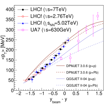
According to the scaling law proposed in Ref. Amati , the average transverse momentum, denoted $\langle p_{\text{T}}\rangle$, as a function of rapidity should be independent of the center-of-mass energy in the projectile fragmentation region. Here we obtain and compare the $\langle p_{\text{T}}\rangle$ distributions as functions of rapidity for $p+p$ and $p+\text{Pb}$ collisions. In the study of this paper, $\langle p_{\text{T}}\rangle$ is obtained by three methods discussed below. The first two methods use analytic distributions that are fit to the LHCf data and the third uses numerical integration of the LHCf data.

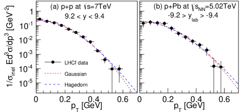
The first method uses the fit of an empirical Gaussian distribution to the LHCf $p_{\text{T}}$ distributions for each rapidity range in Fig. 5, 9, and 13. The second method uses a Hagedorn function. Here we pay attention to the fact that soft scattering dominates the measured $\pi^{0}$ events for $p_{\text{T}}<\sim$1\text{\,}\mathrm{GeV}$$ thus excluding from the analysis a power-law distribution that is used predominantly for hard scattering at $p_{\text{T}}>\sim$1\text{\,}\mathrm{GeV}$$. These methods do not necessarily require that the measured $p_{\text{T}}$ distribution be available down to $0.0\text{\,}\mathrm{GeV}$, although the best-fit distribution may then include a systematic uncertainty in its fit Hagedorn . Detailed descriptions of the parametrization and derivation of $\langle p_{\text{T}}\rangle$ by using the best-fit Gaussian distribution can be found in Ref. LHCfpppi0 . In a Hagedorn function Hagedorn , the invariant cross section of identified hadrons, namely $\pi^{0}$s in this paper, with a given mass $\widehat{m}$ [GeV] and temperature $\widehat{T}$ [GeV] can be written as

$$\frac{1}{\sigma_{\text{inel}}}E\frac{d^{3}\sigma}{dp^{3}}=A\cdot\sqrt{p_{\text{T}}^{2}+\widehat{m}^{2}}\sum_{n=1}^{\infty}K_{1}\left(n\frac{\sqrt{p_{\text{T}}^{2}+\widehat{m}^{2}}}{\widehat{T}}\right),$$ (6)

where $A$ [${\mathrm{GeV}}^{-3}$] is a normalization factor and $K_{1}$ is the modified Bessel function. Approximately half of the $\pi^{0}$ measured with the LHCf detector are daughters from the decay of parent baryons and mesons and are not directly produced. Thus the measured $p_{\text{T}}$ distribution is no longer a thermal distribution of prompt $\pi^{0}$s and so we set $\widehat{m}$ as a free parameter as well as $A$ and $\widehat{T}$ in the fit of a Hagedorn function to the $p_{\text{T}}$ distribution. Equation (6) converges by $n\approx 5$ and the computation is in fact stopped at $n=10$. The $\langle p_{\text{T}}\rangle$ value is calculated by using the modified Bessel functions $K_{5/2}$ and $K_{2}$ as functions of the ratio of the best-fit $\widehat{m}$ and $\widehat{T}$ values Hagedorn ,

$$\langle p_{\text{T}}\rangle=\sqrt{\frac{\pi\widehat{m}\widehat{T}}{2}}\frac{\sum_{n=1}^{\infty}K_{5/2}(n(\widehat{m}/\widehat{T}))}{\sum_{n=1}^{\infty}K_{2}(n(\widehat{m}/\widehat{T}))}.$$ (7)

For reference, Fig. 17 shows LHCf $p_{\text{T}}$ distributions (filled black circles) and the best fits of the Gaussian distributions and the Hagedorn functions. The left panel of Fig. 17 shows the results for $9.2<y<9.4$ in $p+p$ collisions at $\sqrt{s}=$7\text{\,}\mathrm{TeV}$$. The best-fit Gaussian distribution (dotted red curve) and Hagedorn function (dashed blue curve) to the LHCf data mostly overlap each other and give compatible $\langle p_{\text{T}}\rangle$ values. The right panel of Fig. 17 shows the results for $-9.2>y_{\text{lab}}>-9.4$ in $p+\text{Pb}$ collisions at $\sqrt{s_{\textrm{NN}}}=$5.02\text{\,}\mathrm{TeV}$$. Note that the $p_{\text{T}}$ distribution for LHCf data is plotted after subtraction of the UPC component where the systematic uncertainty in the simulation of UPC events has been taken into account. The best-fit Gaussian distribution and the Hagedorn function reproduce the LHCf $p_{\text{T}}$ distributions within the total uncertainties and are also compatible with each other.

Finally, for the third method, $\langle p_{\text{T}}\rangle$ is obtained by numerically integrating the $p_{\text{T}}$ distributions in Fig. 5, 9, and 13. The LHCf $p_{\text{T}}$ distributions in $p+\text{Pb}$ collisions have already had the UPC component subtracted. In this approach, $\langle p_{\text{T}}\rangle$ is calculated only in the rapidity range where the $p_{\text{T}}$ distributions are available down to $0.0\text{\,}\mathrm{GeV}$. The high-$p_{\text{T}}$ tail that extends beyond the data ($p_{\text{T}}\gg\langle p_{\text{T}}\rangle$) has a negligible contribution to $\langle p_{\text{T}}\rangle$. The final $\langle p_{\text{T}}\rangle$ values obtained in this analysis, denoted $\langle p_{\text{T}}\rangle_{\textrm{LHCf}}$, have been determined by averaging the $\langle p_{\text{T}}\rangle$ values calculated with the three above described independent approaches: Gaussian, Hagedorn and numerical integration. The uncertainty of $\langle p_{\text{T}}\rangle_{\textrm{LHCf}}$ for each rapidity bin is assigned to fully cover the minimum and maximum $\langle p_{\text{T}}\rangle$ values obtained by the three approaches. The $\langle p_{\text{T}}\rangle_{\textrm{LHCf}}$ values are summarized in Table. 3.

In Fig. 18, $\langle p_{\text{T}}\rangle$ in $p+p$ collisions at $\sqrt{s}=2.76$ and $7\text{\,}\mathrm{TeV}$, and in $p+\text{Pb}$ collisions at $\sqrt{s_{\textrm{NN}}}=$5.02\text{\,}\mathrm{TeV}$$ are presented as a function of rapidity loss $\Delta y\equiv y_{\text{beam}}-y$, where $y_{\text{beam}}$ is the beam rapidity for each collision energy. The shift in rapidity by $y_{\text{beam}}$ allows a direct comparison to be made between the $\langle p_{\text{T}}\rangle$ results at different collision energies. We see that for $\Delta y>-1.3$, $\langle p_{\text{T}}\rangle$ at $\sqrt{s}=$2.76\text{\,}\mathrm{TeV}$$ (open red circles) has slightly smaller values than at $\sqrt{s}=$7\text{\,}\mathrm{TeV}$$ (filled black circles), although the two sets of data are mostly compatible at the $\pm$10\text{\,}\mathrm{\char 37\relax}$$ level. For reference, the Sp$\bar{\text{p}}$S UA7 results for $p+\bar{p}$ collisions at $\sqrt{s}=$630\text{\,}\mathrm{GeV}$$ UA7 (open magenta squares) show a rapid roll off of $\langle p_{\text{T}}\rangle$ at low $\Delta y$ compared to LHCf data. The LHCf and UA7 results are particularly incompatible for $-0.3<\Delta y<0.3$. The comparison of the LHCf data with the UA7 results indicates that $\langle p_{\text{T}}\rangle$ may depend on the center-of-mass energy. However, in order to firmly confirm a center-of-mass energy dependence of $\langle p_{\text{T}}\rangle$, we need to have experimental data at a lower collision energy, e.g., $\sqrt{s}<$1\text{\,}\mathrm{TeV}$$ and with a wider range of rapidity. Approved plans are underway to obtain this data by installing the LHCf detector at the RHIC ZDC position RHICf . The $\langle p_{\text{T}}\rangle$ values obtained from $p+\text{Pb}$ collisions at $\sqrt{s_{\textrm{NN}}}=$5.02\text{\,}\mathrm{TeV}$$ (filled blue triangles) are consistent with those from $p+p$ collisions at $\sqrt{s}=$7\text{\,}\mathrm{TeV}$$ within the systematic uncertainties present. The predictions from dpmjet (thick solid red line) and qgsjet (thin solid blue line) in $p+p$ collisions at $\sqrt{s}=$7\text{\,}\mathrm{TeV}$$ and $p+\text{Pb}$ collisions at $\sqrt{s_{\textrm{NN}}}=$5.02\text{\,}\mathrm{TeV}$$ have been added to Fig. 18 for reference. The predictions at $\sqrt{s}=$2.76\text{\,}\mathrm{TeV}$$ are excluded in Fig. 18, since these curves mostly overlap with those at $7\text{\,}\mathrm{TeV}$. LHCf data in $p+p$ collisions at $\sqrt{s}=$7\text{\,}\mathrm{TeV}$$ are close to the predictions made by dpmjet at large $\Delta y$ (small $y$) and become close to those made by qgsjet at small $\Delta y$ (large $y$). These relations between LHCf data and the model predictions are consistent with the $p_{\text{T}}$ distributions shown in Fig. 5 and 9. The prediction from dpmjet (thick dashed red line) for $p+\text{Pb}$ collisions at $\sqrt{s_{\textrm{NN}}}=$5.02\text{\,}\mathrm{TeV}$$ is compatible with the LHCf result for $-0.3<\Delta y<0.2$, which is derived from the good agreement of this model with LHCf data at $-8.8>y_{\text{lab}}>-10.0$ and $p_{\text{T}}<$0.3\text{\,}\mathrm{GeV}$$. Conversely, the prediction obtained from qgsjet (thin dashed blue line) is smaller than LHCf data for $\Delta y>-0.5$ and approaches the LHCf results on decreasing $\Delta y$. This tendency was already found in Fig. 13; the prediction from qgsjet shows an overall agreement with LHCf $p_{\text{T}}$ distributions at $y_{\text{lab}}<-9.8$.

Figure 17: (color online). LHCf $p_{\text{T}}$ distributions (filled black circles), the best-fit Gaussian distributions (dotted red curve), and the best-fit Hagedorn functions (dashed blue curve). Left: the data for $p+p$ collisions at $\sqrt{s}=$7\text{\,}\mathrm{TeV}$$. Right: the data for $p+\text{Pb}$ collisions at $\sqrt{s_{\textrm{NN}}}=$5.02\text{\,}\mathrm{TeV}$$.

Figure 18: (color online). Average $p_{\text{T}}$ as a function of rapidity loss $\Delta y=y_{\text{beam}}-y$. Open red circles and filled black circles indicate LHCf data in $p+p$ collisions at $\sqrt{s}=2.76$ and $7\text{\,}\mathrm{TeV}$, respectively. The results of the UA7 experiment (open magenta box) at Sp$\bar{\text{p}}$S ($p+\bar{p}$ collisions at $\sqrt{s}=$630\text{\,}\mathrm{GeV}$$) and the predictions from dpmjet (thick lines) and qgsjet (thin lines) are added for reference.

Table 3: The average $\pi^{0}$ transverse momenta for the rapidity range $8.8<y<10.6$ in $p+p$ collisions at $\sqrt{s}=2.76$ and $7\text{\,}\mathrm{TeV}$ and for the rapidity range $-8.8>y_{\text{lab}}>-10.6$ in $p+\text{Pb}$ collisions at $\sqrt{s_{\textrm{NN}}}=$5.02\text{\,}\mathrm{TeV}$$.

Rapidity	$\langle p_{\text{T}}\rangle_{\textrm{LHCf}}$ [MeV]
	$p+p~{}$2.76\text{\,}\mathrm{TeV}$$	$p+p~{}$7\text{\,}\mathrm{TeV}$$	$p+\text{Pb}~{}$5.02\text{\,}\mathrm{TeV}$$
$[$8.8, 9.0$]$	$103.5\pm 7.5$0	$242.8\pm 8.6$	$244.5\pm 43.2$
$[$9.0, 9.2$]$	0$78.5\pm 7.8$0	$208.5\pm 6.1$	$223.1\pm 12.7$
$[$9.2, 9.4$]$	0$76.4\pm 5.7$0	$182.6\pm 4.3$	$189.9\pm 7.6$0
$[$9.4, 9.6$]$	0$60.3\pm 5.2$0	$160.2\pm 3.8$	$173.8\pm 17.2$
$[$9.6, 9.8$]$	0$50.4\pm 10.4$	$132.3\pm 3.4$	$138.1\pm 18.7$
$[$9.8, 10.0$]$		$113.9\pm 3.4$	$113.0\pm 6.3$0
$[$10.0,10.2$]$		0$87.3\pm 3.9$	$112.2\pm 15.4$
$[$10.2,10.4$]$		0$67.5\pm 3.0$	0$90.7\pm 6.7$0
$[$10.4,10.6$]$		0$55.6\pm 3.1$	0$61.0\pm 6.6$0

VII.2 Limiting fragmentation

The hypothesis of limiting fragmentation Limiting1 ; Limiting2 ; Limiting3 asserts that the number of fragments of a colliding hadron will follow a limiting rapidity distribution in the rest frame of the target hadron. In this case the rapidity distribution of the secondary particles in the forward rapidity region would be independent of the center-of-mass energy. In this paper, a test of the limiting fragmentation hypothesis is performed by using LHCf data in $p+p$ collisions at $\sqrt{s}=2.76$ and $7\text{\,}\mathrm{TeV}$.

The normalized rapidity distribution of $\pi^{0}$s, $(1/\sigma_{\text{inel}})(d\sigma/dy)$, in this analysis can be obtained by using very similar methods that were used for the derivation of the average $p_{\text{T}}$ in Sec. VII.1.

The first method uses the fit of an empirical distribution to the LHCf $p_{\text{T}}$ distributions in Fig. 5 and 9 in each rapidity range. As we discussed in Sec. VII.1, two distributions are chosen to parametrize the $p_{\text{T}}$ distributions: a Gaussian distribution and a Hagedorn function. The rapidity distribution is derived by integrating the best-fit Gaussian distribution and Hagedorn function along the $p_{\text{T}}$ axis from $0.0\text{\,}\mathrm{GeV}$ to infinity.

The rapidity distribution can also be obtained by numerically integrating the $p_{\text{T}}$ distributions in Fig. 5 and 9. In this approach, the derivation of the $(1/\sigma_{\text{inel}})(d\sigma/dy)$ value is possible only in the rapidity range where the $p_{\text{T}}$ distributions are available down to $0.0\text{\,}\mathrm{GeV}$. Again, the final rapidity distribution is derived by averaging the rapidity distributions obtained by the above three methods. The estimated uncertainty is obtained from the minimum and maximum values for each rapidity bin.

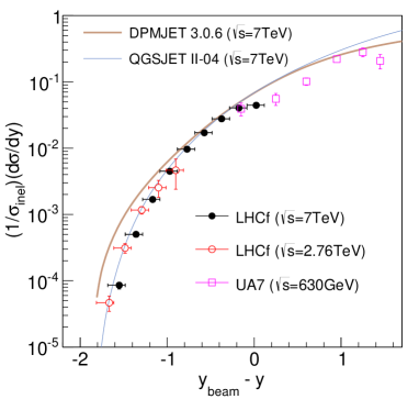
Figure 19 shows the rapidity distributions as functions of the rapidity loss $\Delta y$ (i.e., $y_{\text{beam}}-y$) in $p+p$ collisions at $\sqrt{s}=$2.76\text{\,}\mathrm{TeV}$$ (open red circles) and $7\text{\,}\mathrm{TeV}$ (filled black circles). The rapidity distributions for both collision energies mostly appear to lie along a common curve in the rapidity range $-1.8<\Delta y<-0.8$. LHCf data are consistent at the $\pm$15\text{\,}\mathrm{\char 37\relax}$$ level with the hypothesis of limiting fragmentation in the very forward region.

For comparison the experimental results from the UA7 experiment UA7 are also shown in Fig. 19. The extrapolated LHCf curve at $7\text{\,}\mathrm{TeV}$ to higher $\Delta y$ (i.e., lower $y$) could be compatible with the UA7 results, at least for $\Delta y\lesssim 0.5$.

The predictions of dpmjet (thick red curve) and qgsjet (thin blue curve) at $\sqrt{s}=$7\text{\,}\mathrm{TeV}$$ have been added to Fig. 19 for reference. The predictions at $\sqrt{s}=$2.76\text{\,}\mathrm{TeV}$$ have been omitted, since these curves mostly overlap with those at $7\text{\,}\mathrm{TeV}$ since limiting fragmentation holds in dpmjet and qgsjet. The best agreement with LHCf data at $\sqrt{s}=2.76$ and $7\text{\,}\mathrm{TeV}$ is obtained by the qgsjet model. The dpmjet predictions generally give a larger $\pi^{0}$ yield and a harder $p_{\text{T}}$ distribution especially for $y>9.8$ at $\sqrt{s}=$7\text{\,}\mathrm{TeV}$$ and for $y>9.4$ at $2.76\text{\,}\mathrm{TeV}$.

Figure 19: (color online). The $\pi^{0}$ yield in each rapidity interval as a function of rapidity loss $\Delta y=y_{\text{beam}}-y$. Open red circles and filled black circles indicate LHCf data in $p+p$ collisions at $\sqrt{s}=2.76$ and $7\text{\,}\mathrm{TeV}$, respectively. The results of the UA7 experiment (open magenta squares) at Sp$\bar{\text{p}}$S ($p+\bar{p}$ collisions at $\sqrt{s}=$630\text{\,}\mathrm{GeV}$$) and the predictions by dpmjet (thick red line) and qgsjet (thin blue line) are added for reference.

VII.3 Feynman scaling

In Ref. Feynman Feynman proposed that the production cross sections of secondary particles as functions of the Feynman-x variable (defined by $x_{F}\equiv 2p_{\text{z}}/\sqrt{s}$) were independent of the incident energy in the forward region. If the so-called Feynman scaling holds, the differential cross section as a function of $x_{F}$ (hereafter $x_{F}$ distribution) $(x_{F}/\sigma_{\text{inel}})(d\sigma/dx_{F})$ should be independent of the center-of-mass energy for $x_{F}\gtrsim 0.2$. Here the rapidity distribution introduced in Sec. VII.2 can be rewritten as

$$\frac{1}{\sigma_{\text{inel}}}\frac{d\sigma}{dy}=\frac{E}{\sigma_{\text{inel}}}\frac{d\sigma}{dp_{\text{z}}}=\frac{x_{E}}{\sigma_{\text{inel}}}\frac{d\sigma}{dx_{F}},$$ (8)

where $x_{E}\equiv 2E/\sqrt{s}$ and $dy=dp_{\text{z}}/E$ are used for the second form. Considering $p_{\text{z}}\approx E$ in the forward region, $x_{E}$ can be considered as $x_{F}$ and thus the right hand side of Eq. (8) becomes approximately $(x_{F}/\sigma_{\text{inel}})(d\sigma/dx_{F})$. Consequently, the limiting fragmentation hypothesis that states $(1/\sigma_{\text{inel}})(d\sigma/dy)$ is independent of the center-of-mass energy in each rapidity bin can be rewritten as Feynman scaling which states $(x_{F}/\sigma_{\text{inel}})(d\sigma/dx_{F})$ is independent of the center-of-mass energy in each $x_{F}$ bin. In this paper, we test the Feynman scaling hypothesis by comparing LHCf data in $p+p$ collisions at $\sqrt{s}=2.76$ and $7\text{\,}\mathrm{TeV}$.

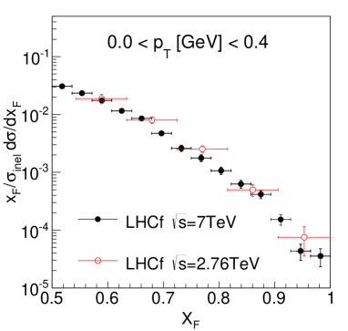
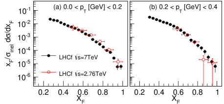
In Fig. 20, we compare the $x_{F}$ distributions in the $p_{\text{T}}$ range $0.0<p_{\text{T}}<$0.4\text{\,}\mathrm{GeV}$$. Other $p_{\text{T}}$ ranges are excluded from the comparison, since LHCf data at $\sqrt{s}=$2.76\text{\,}\mathrm{TeV}$$ are unavailable outside this range. The $x_{F}$ distributions at $\sqrt{s}=2.76$ and $7\text{\,}\mathrm{TeV}$ are compatible with each other at the $\pm$20\text{\,}\mathrm{\char 37\relax}$$ level. In Fig. 21, we further compare the $x_{F}$ distributions for the reduced $p_{\text{T}}$ ranges: $0.0<p_{\text{T}}<$0.2\text{\,}\mathrm{GeV}$$ and $0.2<p_{\text{T}}<$0.4\text{\,}\mathrm{GeV}$$. At $0.0<p_{\text{T}}<$0.2\text{\,}\mathrm{GeV}$$, only the bin $0.73<x_{F}<0.82$ at $\sqrt{s}=$2.76\text{\,}\mathrm{TeV}$$ deviates from the one at $7\text{\,}\mathrm{TeV}$ by $30\text{\,}\mathrm{\char 37\relax}$, while the other bins are consistent within their uncertainties. At $0.2<p_{\text{T}}<$0.4\text{\,}\mathrm{GeV}$$, all bins at $\sqrt{s}=$2.76\text{\,}\mathrm{TeV}$$ are consistent with the ones at $7\text{\,}\mathrm{TeV}$, except for the bin $0.82<x_{F}<0.91$ that has a smaller ($40\text{\,}\mathrm{\char 37\relax}$) cross section than at $7\text{\,}\mathrm{TeV}$, although there is a large uncertainty at $2.76\text{\,}\mathrm{TeV}$. Overall the $x_{F}$ distributions at $\sqrt{s}=2.76$ and $7\text{\,}\mathrm{TeV}$ indicate that Feynman scaling holds at the $\pm$20\text{\,}\mathrm{\char 37\relax}$$ level at these center-of-mass energies in the very forward region.

Besides a test of the Feynman scaling, we find in Fig. 21 that the yield of $\pi^{0}$s at $\sqrt{s}=$2.76\text{\,}\mathrm{TeV}$$ relative to $7\text{\,}\mathrm{TeV}$ is slightly larger for $0.0<p_{\text{T}}<$0.2\text{\,}\mathrm{GeV}$$ and slightly smaller for $0.2<p_{\text{T}}<$0.4\text{\,}\mathrm{GeV}$$. This tendency means that the $p_{\text{T}}$ distributions at $\sqrt{s}=$2.76\text{\,}\mathrm{TeV}$$ are softer than those at $7\text{\,}\mathrm{TeV}$, leading to the small $\langle p_{\text{T}}\rangle$ values at $2.76\text{\,}\mathrm{TeV}$ relative to those at $7\text{\,}\mathrm{TeV}$ as already found in Fig. 18.

Figure 20: (color online). The $\pi^{0}$ yield at $0.0<p_{\text{T}}<$0.4\text{\,}\mathrm{GeV}$$ as a function of $x_{F}$. Open red circles and filled black circles indicate LHCf data in $p+p$ collisions at $\sqrt{s}=2.76$ and $7\text{\,}\mathrm{TeV}$, respectively.

Figure 21: (color online). The $\pi^{0}$ yield in each $p_{\text{T}}$ range as a function of $x_{F}$. Left: the distributions for $0.0<p_{\text{T}}<$0.2\text{\,}\mathrm{GeV}$$. Right: the distributions for $0.2<p_{\text{T}}<$0.4\text{\,}\mathrm{GeV}$$. Open red circles and filled black circles indicate LHCf data in $p+p$ collisions at $\sqrt{s}=2.76$ and $7\text{\,}\mathrm{TeV}$, respectively.

VII.4 $p_{\text{T}}$ dependence of the $x_{F}$ distributions

In hadronic interactions at large rapidities, partons from the projectile and target hadrons generally have large and small momentum fractions respectively, since the momentum fraction that the parton itself carries relative to the parent projectile and target hadrons, i.e., the Bjorken-$x$ variable or $x_{Bj}$, is proportional to $e^{\pm y}$ ($+y$ for projectile and $-y$ for target). Here we note that a parton (dominantly gluon) density, rapidly increases with decreasing $x_{Bj}$ when $x_{Bj}<0.01$ with the target approaching the blackbody limit where the gluon density is saturated. In the blackbody regime, the partons cannot go through the target nuclear medium without interaction and suffer transverse momenta transfers proportional to the saturation momentum scale $Q_{s}$. The $Q_{s}$ values in the very forward region are $\sim$1\text{\,}\mathrm{GeV}$$ in $p+p$ collisions and $\sim$10\text{\,}\mathrm{GeV}$$ in $p+\text{Pb}$ collisions, although the calculation of $Q_{s}$ itself suffers from both theoretical and experimental uncertainties and is also dependent on the impact parameter of the colliding hadrons Albacete .

In the $p_{\text{T}}$ region below $Q_{s}$, the $x_{F}$ distribution in the forward region can be asymptotically written Berera as

$$\frac{x_{F}}{\sigma_{\text{inel}}}\frac{d\sigma}{dx_{F}}\propto(1-x_{F})^{\alpha}.$$ (9)

where $\alpha$ is the leading exponent. In the blackbody regime, the $x_{F}$ distribution of the leading hadron is strongly suppressed and thus $\alpha$ increases relative to the value found for a dilute target. Conversely, $\alpha$ decreases with increasing $p_{\text{T}}$ when $p_{\text{T}}$ approaches or exceeds the saturation momentum scale $Q_{s}$.

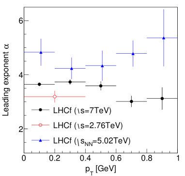
Figure 22 shows the best-fit leading exponent $\alpha$ in each $p_{\text{T}}$ range in $p+p$ and $p+\text{Pb}$ collisions. The leading exponent in $p+p$ collisions at $\sqrt{s}=$7\text{\,}\mathrm{TeV}$$ (filled black circles) is $\alpha\approx 3.7$ at $p_{\text{T}}<$0.6\text{\,}\mathrm{GeV}$$ and decreases to $\alpha\approx 3.0$ at $0.6<p_{\text{T}}<$1.0\text{\,}\mathrm{GeV}$$. The reduction of $\alpha$ with increasing $p_{\text{T}}$ can be understood as much of the target staying in the blackbody regime for $p_{\text{T}}<$0.6\text{\,}\mathrm{GeV}$$ and then gradually escaping from the blackbody regime for $p_{\text{T}}>$0.6\text{\,}\mathrm{GeV}$$. The leading exponent in $p+p$ collisions at $\sqrt{s}=$2.76\text{\,}\mathrm{TeV}$$ (open red circles) is slightly smaller than that at $7\text{\,}\mathrm{TeV}$ though with large uncertainty. The comparison between $\sqrt{s}=$2.76\text{\,}\mathrm{TeV}$$ and $7\text{\,}\mathrm{TeV}$ may indicate that the upper $p_{\text{T}}$ limit of the measurement at $2.76\text{\,}\mathrm{TeV}$ is near the saturation momentum at $2.76\text{\,}\mathrm{TeV}$ and that the suppression due to the gluon density is weaker than at $7\text{\,}\mathrm{TeV}$, although the calculated $Q_{s}$ at $2.76\text{\,}\mathrm{TeV}$ is only slightly different from the $Q_{s}$ at $7\text{\,}\mathrm{TeV}$. The leading exponents in $p+\text{Pb}$ collisions at $\sqrt{s_{\textrm{NN}}}=$5.02\text{\,}\mathrm{TeV}$$ (filled blue triangles) are rather flat along the $p_{\text{T}}$ axis, within uncertainties that are generally larger than those in $p+p$ collisions. This may indicate that the saturation momentum in $p+\text{Pb}$ collisions is well above the measured $p_{\text{T}}$ range and also that the $x_{F}$ distributions in $p+\text{Pb}$ collisions are suppressed relative to those for $p+p$ collisions.

Figure 22: (color online). The best-fit leading exponent of (1-$x_{F}$) as a function of $p_{\text{T}}$. Open red circles and filled black circles indicate LHCf data in $p+p$ collisions at $\sqrt{s}=2.76$ and $7\text{\,}\mathrm{TeV}$, respectively. Filled blue triangles indicate LHCf data in $p+\text{Pb}$ collisions at $\sqrt{s_{\textrm{NN}}}=$5.02\text{\,}\mathrm{TeV}$$.

VII.5 Nuclear modification factor

The effects of high gluon density in the target are inferred from the comparison of the leading exponent $\alpha$ between in $p+p$ and $p+\text{Pb}$ collisions (see the preceding Sec. VII.4). Here we introduce the nuclear modification factor that quantifies the $p_{\text{T}}$ spectra modification caused by nuclear effects in $p+\text{Pb}$ collisions with respect to $p+p$ collisions. The nuclear modification factor $R_{\textrm{pPb}}$ is defined as

$$R_{\textrm{pPb}}\equiv\frac{\sigma^{\textrm{pp}}_{\textrm{inel}}}{\langle N_{\textrm{coll}}\rangle\sigma^{\textrm{pPb}}_{\textrm{inel}}}\frac{Ed^{3}\sigma^{\textrm{pPb}}/dp^{3}}{Ed^{3}\sigma^{\textrm{pp}}/dp^{3}},$$ (10)

where $Ed^{3}\sigma^{\text{pPb}}/dp^{3}$ and $Ed^{3}\sigma^{\text{pp}}/dp^{3}$ are the inclusive cross sections of $\pi^{0}$ production in $p+\text{Pb}$ collisions at $\sqrt{s_{\textrm{NN}}}=$5.02\text{\,}\mathrm{TeV}$$ and in $p+p$ collisions at $\sqrt{s}=$5.02\text{\,}\mathrm{TeV}$$, respectively. These cross sections are obtained from Eq. (5) and Eq. (1), with the subtraction of the expected UPC contribution applied to the cross section for $p+\text{Pb}$ collisions. The uncertainty in the inelastic cross section $\sigma^{\text{pPb}}_{\text{inel}}$ is estimated to be $\pm$5\text{\,}\mathrm{\char 37\relax}$$ LHCfpPbpi0 . The average number of binary nucleon–nucleon collisions in a $p+\text{Pb}$ collision, $\langle N_{\textrm{coll}}\rangle=6.9$, is obtained from MC simulations using the Glauber model dEnterria . The uncertainty of $\sigma^{\textrm{pp}}_{\textrm{inel}}/\langle N_{\textrm{coll}}\rangle$ is estimated by varying the parameters in the calculation with the Glauber model and is of the order of $\pm$3.5\text{\,}\mathrm{\char 37\relax}$$ LHCfpPbpi0 . Finally the quadratic sum of the uncertainties in $\sigma^{\text{pPb}}_{\text{inel}}$ and $\sigma^{\textrm{pp}}_{\textrm{inel}}/\langle N_{\textrm{coll}}\rangle$ is added to $R_{\textrm{pPb}}$.

Since there is no LHCf data for $p+p$ collisions at exactly $\sqrt{s}=$5.02\text{\,}\mathrm{TeV}$$, $Ed^{3}\sigma^{\text{pp}}/dp^{3}$ is derived by scaling the $p_{\text{T}}$ distributions taken in $p+p$ collisions to other collision energies. The derivation follows three steps. First, the $\langle p_{\text{T}}\rangle$ at $\sqrt{s}=$5.02\text{\,}\mathrm{TeV}$$ is estimated by interpolating the measured $\langle p_{\text{T}}\rangle$ values at $7\text{\,}\mathrm{TeV}$. The uncertainty of the interpolated $\langle p_{\text{T}}\rangle$ values is estimated to be $\pm$10\text{\,}\mathrm{\char 37\relax}$$ according to the differences between the measured $\langle p_{\text{T}}\rangle$ values at $\sqrt{s}=2.76$ and $7\text{\,}\mathrm{TeV}$ for $-1.7<\Delta y<-0.8$ (see Fig. 18). Second, the absolute normalization of the $p_{\text{T}}$ distribution value in each rapidity range for $\sqrt{s}=$5.02\text{\,}\mathrm{TeV}$$, i.e., $(1/\sigma_{\text{inel}})(d\sigma/dy)$, is determined by interpolating the rapidity distribution at $7\text{\,}\mathrm{TeV}$ (see Fig. 19). The uncertainty of the absolute normalization is estimated to be $\pm$15\text{\,}\mathrm{\char 37\relax}$$ according to the discussion in Sec. VII.2 and is taken into account in the interpolated normalization. Finally, the $p_{\text{T}}$ distributions at $\sqrt{s}=$5.02\text{\,}\mathrm{TeV}$$ are produced by assuming that the $p_{\text{T}}$ distribution follows either a Gaussian distribution or a Hagedorn function and by using the $\langle p_{\text{T}}\rangle$ values obtained in the first step and the normalization obtained in the second step. The difference of the $p_{\text{T}}$ distribution produced using a Gaussian distribution or a Hagedorn function gives the systematic uncertainty. Note that the rapidity shift $-0.465$ explained in Sec. III.2 is also taken into account for the $p_{\text{T}}$ distribution in $p+p$ collisions at $\sqrt{s}=$5.02\text{\,}\mathrm{TeV}$$.

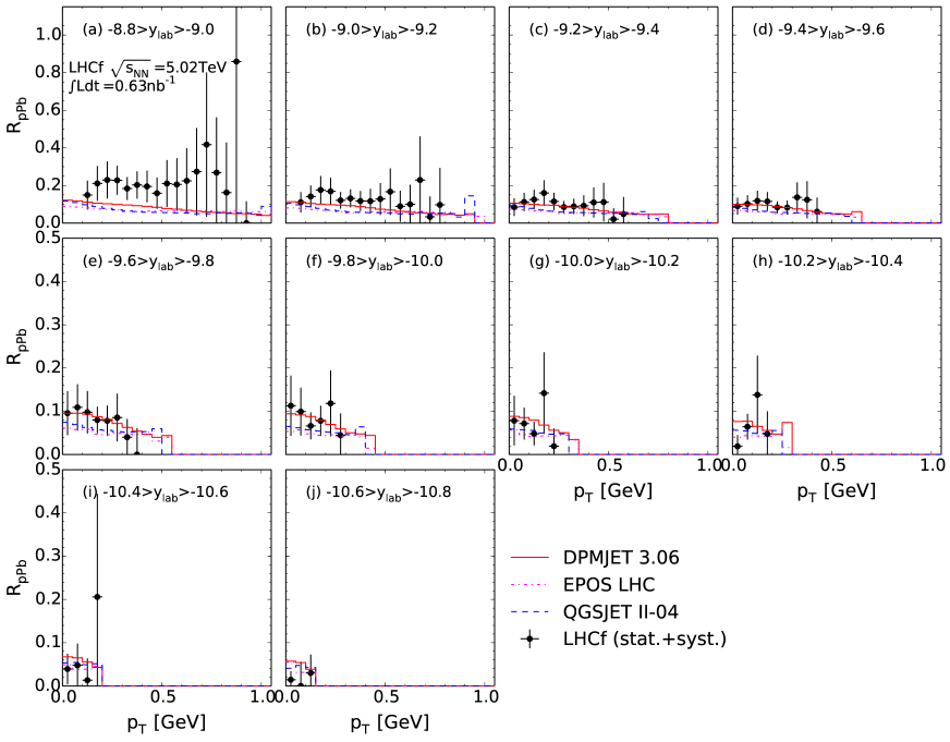
Figure 23 shows the nuclear modification factors $R_{\textrm{pPb}}$ obtained from LHCf data and the predictions from the hadronic interaction models, dpmjet (solid red curve), qgsjet (dashed blue curve), and epos (dotted magenta curve). LHCf data show a strong suppression with $R_{\textrm{pPb}}$ equal to 0.3 at $y_{\text{lab}}\sim-8.8$ down to $<0.1$ at $y_{\text{lab}}\sim-10.8$, although a large uncertainty is present due to systematic uncertainties in the estimation of the $\langle p_{\text{T}}\rangle$ values in $p+p$ collisions at $\sqrt{s}=$5.02\text{\,}\mathrm{TeV}$$. All hadronic interaction models, which employ different approaches for the nuclear effects, predict small values of $R_{\textrm{pPb}}\lesssim 0.15$. Within the uncertainties the hadronic interaction models show an overall good agreement with $R_{\textrm{pPb}}$ estimated from LHCf data.

Figure 23: (color online). The nuclear modification factor for $\pi^{0}$s. Filled circles indicate the factors obtained from LHCf data. Error bars indicate the total uncertainties incorporating both statistical and systematic uncertainties. Other lines are the predictions from hadronic interaction models: dpmjet (solid red line), qgsjet (dashed blue line), and epos (dashed-dotted magenta line).

VIII Conclusions

The inclusive production of $\pi^{0}$s was measured with the LHCf detector in $p+p$ collisions at $\sqrt{s}=2.76$ and $7\text{\,}\mathrm{TeV}$ and in $p+\text{Pb}$ collisions at $\sqrt{s_{\textrm{NN}}}=$5.02\text{\,}\mathrm{TeV}$$. In $p+p$ collisions at $\sqrt{s}=$7\text{\,}\mathrm{TeV}$$, differential cross sections as a function of $p_{\text{T}}$ and $p_{\text{z}}$ for the $\pi^{0}$s were measured by two independent LHCf detectors, Arm1 and Arm2, with consistent results. Conversely, only the LHCf Arm2 detector was used in $p+p$ collisions at $\sqrt{s}=$2.76\text{\,}\mathrm{TeV}$$ and in $p+\text{Pb}$ collisions.

In $p+p$ collisions, qgsjet II-04 shows an overall agreement with LHCf data, while epos lhc distributions have a slightly harder behavior than LHCf data for $p_{\text{T}}>$0.5\text{\,}\mathrm{GeV}$$. dpmjet 3.06 and pythia 8.185 have in general shown a harder momentum distributions and a poor agreement with LHCf data. In $p+\text{Pb}$ collisions, dpmjet 3.06 showed good agreement with LHCf data for $-8.8>y_{\text{lab}}>-10.0$ and $p_{\text{T}}<$0.3\text{\,}\mathrm{GeV}$$, while qgsjet II-04 and epos lhc did better reproducing the LHCf data for $p_{\text{T}}>$0.4\text{\,}\mathrm{GeV}$$ than dpmjet 3.06.

The average values of $p_{\text{T}}$, denoted $\langle p_{\text{T}}\rangle$, at $y>8.8$ in $p+p$ collisions and at $y_{\text{lab}}>8.8$ in $p+\text{Pb}$ collisions were calculated using the LHCf $p_{\text{T}}$ distributions. The $\langle p_{\text{T}}\rangle$ values obtained have been shown to be independent of the center-of-mass energy at the $10\text{\,}\mathrm{\char 37\relax}$ level. Tests of limiting fragmentation and Feynman scaling hypotheses using LHCf data in $p+p$ collisions show that both hypotheses hold in the forward region at the $15\text{\,}\mathrm{\char 37\relax}$–$20\text{\,}\mathrm{\char 37\relax}$ level. The leading exponent $\alpha$ and the nuclear modification factor $R_{\textrm{pPb}}$ derived from LHCf data indicate a strong suppression of $\pi^{0}$ production from the nuclear target relative to that from the nucleon target. Within the uncertainties all of the hadronic interaction models presented gave an overall good agreement with $R_{\textrm{pPb}}$ estimated by LHCf data. According to the analysis in this paper, we expect that the number of particles leading to an electromagnetic component in air showers would follow the limiting rapidity distribution and Feynman scaling hypotheses. Combining the results for forward $\pi^{0}$s in this paper with the recent results for forward neutrons in Ref. LHCfneutron strongly constrain models for air shower production at the TeV scale.

As a future prospect, additional analyses using correlations between forward $\pi^{0}$s and other particles (e.g., two-particle angular correlations) are needed to reach a better understanding of the forward meson production mechanism and the strong suppression of $\pi^{0}$ production in $p+\text{Pb}$ collisions compared to $p+p$ collisions. The ATLAS and LHCf Collaborations have taken $p+p$ data at $\sqrt{s}=$13\text{\,}\mathrm{TeV}$$ and $p+\text{Pb}$ data at $\sqrt{s_{\textrm{NN}}}=$5.02\text{\,}\mathrm{TeV}$$ with common triggers. This data could provide the possibility for performing analyses of two particle correlations.

Appendix: Data tables

The inclusive production rates of $\pi^{0}$s measured by LHCf with all corrections applied are summarized in Tables 4– 18. The ratios of $\pi^{0}$ production rate of MC simulation to data are summarized in Tables 19– 55. The LHCf $p_{\text{T}}$ distributions for $p+\text{Pb}$ collisions have the UPC component subtracted. The nuclear modification factor of $\pi^{0}$s obtained from LHCf data are summarized in Tables 56– 59.

Table 4: Production rate for the $\pi^{0}$ production in the rapidity range $8.8<y<9.0$ in $p+p$ collisions and in the rapidity range $-8.8>y_{\text{lab}}>-9.0$ in $p+\text{Pb}$ collisions. The rate and corresponding total uncertainty are in units of [GeV^-2].

$p_{\text{T}}$ range $[$GeV$]$	$p+p$ at $\sqrt{s}=$2.76\text{\,}\mathrm{TeV}$$		$p+p$ at $\sqrt{s}=$7\text{\,}\mathrm{TeV}$$		$p+\text{Pb}$ at $\sqrt{s_{\textrm{NN}}}=$5.02\text{\,}\mathrm{TeV}$$
	Production rate	Total error	Production rate	Total error	Production rate	Total error
$[$0.10,0.15$]$	3.71$\times 10^{-2}$	$\pm$8.99$\times 10^{-3}$	2.56$\times 10^{-1}$	$\pm$3.75$\times 10^{-2}$	1.63$\times 10^{-1}$	$\pm$5.65$\times 10^{-2}$
$[$0.15,0.20$]$	1.92$\times 10^{-2}$	$\pm$3.36$\times 10^{-3}$	1.98$\times 10^{-1}$	$\pm$2.05$\times 10^{-2}$	1.86$\times 10^{-1}$	$\pm$4.19$\times 10^{-2}$
$[$0.20,0.25$]$	3.47$\times 10^{-3}$	$\pm$7.22$\times 10^{-4}$	1.20$\times 10^{-1}$	$\pm$1.29$\times 10^{-2}$	1.52$\times 10^{-1}$	$\pm$2.76$\times 10^{-2}$
$[$0.25,0.30$]$	5.67$\times 10^{-4}$	$\pm$2.49$\times 10^{-4}$	6.96$\times 10^{-2}$	$\pm$5.65$\times 10^{-3}$	1.06$\times 10^{-1}$	$\pm$1.52$\times 10^{-2}$
$[$0.30,0.35$]$			3.94$\times 10^{-2}$	$\pm$3.43$\times 10^{-3}$	5.59$\times 10^{-2}$	$\pm$8.43$\times 10^{-3}$
$[$0.35,0.40$]$			2.23$\times 10^{-2}$	$\pm$2.28$\times 10^{-3}$	3.80$\times 10^{-2}$	$\pm$6.14$\times 10^{-3}$
$[$0.40,0.45$]$			1.26$\times 10^{-2}$	$\pm$1.52$\times 10^{-3}$	2.13$\times 10^{-2}$	$\pm$3.86$\times 10^{-3}$
$[$0.45,0.50$]$			7.06$\times 10^{-3}$	$\pm$8.82$\times 10^{-4}$	9.51$\times 10^{-3}$	$\pm$1.84$\times 10^{-3}$
$[$0.50,0.55$]$			4.21$\times 10^{-3}$	$\pm$4.93$\times 10^{-4}$	6.56$\times 10^{-3}$	$\pm$1.09$\times 10^{-3}$
$[$0.55,0.60$]$			2.31$\times 10^{-3}$	$\pm$2.61$\times 10^{-4}$	3.18$\times 10^{-3}$	$\pm$5.64$\times 10^{-4}$
$[$0.60,0.65$]$			1.15$\times 10^{-3}$	$\pm$1.44$\times 10^{-4}$	1.64$\times 10^{-3}$	$\pm$3.28$\times 10^{-4}$
$[$0.65,0.70$]$			4.36$\times 10^{-4}$	$\pm$7.06$\times 10^{-5}$	8.98$\times 10^{-4}$	$\pm$1.95$\times 10^{-4}$
$[$0.70,0.75$]$			2.12$\times 10^{-4}$	$\pm$4.56$\times 10^{-5}$	5.88$\times 10^{-4}$	$\pm$1.60$\times 10^{-4}$
$[$0.75,0.80$]$			1.38$\times 10^{-4}$	$\pm$3.15$\times 10^{-5}$	1.54$\times 10^{-4}$	$\pm$7.96$\times 10^{-5}$
$[$0.80,0.85$]$			3.98$\times 10^{-5}$	$\pm$1.59$\times 10^{-5}$	3.63$\times 10^{-5}$	$\pm$4.26$\times 10^{-5}$
$[$0.85,0.90$]$			4.52$\times 10^{-6}$	$\pm$3.26$\times 10^{-6}$	7.07$\times 10^{-5}$	$\pm$4.06$\times 10^{-5}$
$[$0.90,0.95$]$			7.09$\times 10^{-6}$	$\pm$4.54$\times 10^{-6}$	$<1.48$$\times 10^{-6}$

Table 5: Production rate for the $\pi^{0}$ production in the rapidity range $9.0<y<9.2$ in $p+p$ collisions and in the rapidity range $-9.0>y_{\text{lab}}>-9.2$ in $p+\text{Pb}$ collisions. The rate and corresponding total uncertainty are in units of [GeV^-2].

$p_{\text{T}}$ range $[$GeV$]$	$p+p$ at $\sqrt{s}=$2.76\text{\,}\mathrm{TeV}$$		$p+p$ at $\sqrt{s}=$7\text{\,}\mathrm{TeV}$$		$p+\text{Pb}$ at $\sqrt{s_{\textrm{NN}}}=$5.02\text{\,}\mathrm{TeV}$$
	Production rate	Total error	Production rate	Total error	Production rate	Total error
$[$0.05,0.10$]$	4.26$\times 10^{-2}$	$\pm$1.08$\times 10^{-2}$	2.98$\times 10^{-1}$	$\pm$4.72$\times 10^{-2}$	1.66$\times 10^{-1}$	$\pm$5.08$\times 10^{-2}$
$[$0.10,0.15$]$	2.18$\times 10^{-2}$	$\pm$3.74$\times 10^{-3}$	2.27$\times 10^{-1}$	$\pm$2.58$\times 10^{-2}$	1.78$\times 10^{-1}$	$\pm$3.66$\times 10^{-2}$
$[$0.15,0.20$]$	4.20$\times 10^{-3}$	$\pm$7.14$\times 10^{-4}$	1.42$\times 10^{-1}$	$\pm$1.12$\times 10^{-2}$	1.69$\times 10^{-1}$	$\pm$2.97$\times 10^{-2}$
$[$0.20,0.25$]$	2.89$\times 10^{-4}$	$\pm$1.59$\times 10^{-4}$	8.48$\times 10^{-2}$	$\pm$6.20$\times 10^{-3}$	1.14$\times 10^{-1}$	$\pm$2.10$\times 10^{-2}$
$[$0.25,0.30$]$			5.50$\times 10^{-2}$	$\pm$4.43$\times 10^{-3}$	5.31$\times 10^{-2}$	$\pm$8.70$\times 10^{-3}$
$[$0.30,0.35$]$			3.28$\times 10^{-2}$	$\pm$3.02$\times 10^{-3}$	3.46$\times 10^{-2}$	$\pm$5.49$\times 10^{-3}$
$[$0.35,0.40$]$			1.53$\times 10^{-2}$	$\pm$1.59$\times 10^{-3}$	1.73$\times 10^{-2}$	$\pm$3.28$\times 10^{-3}$
$[$0.40,0.45$]$			6.83$\times 10^{-3}$	$\pm$8.38$\times 10^{-4}$	9.01$\times 10^{-3}$	$\pm$2.06$\times 10^{-3}$
$[$0.45,0.50$]$			3.31$\times 10^{-3}$	$\pm$4.19$\times 10^{-4}$	4.87$\times 10^{-3}$	$\pm$1.15$\times 10^{-3}$
$[$0.50,0.55$]$			1.35$\times 10^{-3}$	$\pm$1.74$\times 10^{-4}$	2.96$\times 10^{-3}$	$\pm$6.76$\times 10^{-4}$
$[$0.55,0.60$]$			7.21$\times 10^{-4}$	$\pm$8.11$\times 10^{-5}$	6.98$\times 10^{-4}$	$\pm$2.73$\times 10^{-4}$
$[$0.60,0.65$]$			1.94$\times 10^{-4}$	$\pm$4.84$\times 10^{-5}$	3.24$\times 10^{-4}$	$\pm$1.66$\times 10^{-4}$
$[$0.65,0.70$]$			9.56$\times 10^{-5}$	$\pm$2.79$\times 10^{-5}$	2.92$\times 10^{-4}$	$\pm$1.13$\times 10^{-4}$
$[$0.70,0.75$]$			1.26$\times 10^{-5}$	$\pm$5.76$\times 10^{-6}$	1.56$\times 10^{-5}$	$\pm$4.63$\times 10^{-5}$
$[$0.75,0.80$]$			5.05$\times 10^{-6}$	$\pm$3.11$\times 10^{-6}$	1.60$\times 10^{-5}$	$\pm$2.68$\times 10^{-5}$

Table 6: Production rate for the $\pi^{0}$ production in the rapidity range $9.2<y<9.4$ in $p+p$ collisions and in the rapidity range $-9.2>y_{\text{lab}}>-9.4$ in $p+\text{Pb}$ collisions. The rate and corresponding total uncertainty are in units of [GeV^-2].

$p_{\text{T}}$ range $[$GeV$]$	$p+p$ at $\sqrt{s}=$2.76\text{\,}\mathrm{TeV}$$		$p+p$ at $\sqrt{s}=$7\text{\,}\mathrm{TeV}$$		$p+\text{Pb}$ at $\sqrt{s_{\textrm{NN}}}=$5.02\text{\,}\mathrm{TeV}$$
	Production rate	Total error	Production rate	Total error	Production rate	Total error
$[$0.00,0.05$]$	4.46$\times 10^{-2}$	$\pm$1.33$\times 10^{-2}$	2.74$\times 10^{-1}$	$\pm$5.08$\times 10^{-2}$	1.46$\times 10^{-1}$	$\pm$5.35$\times 10^{-2}$
$[$0.05,0.10$]$	2.07$\times 10^{-2}$	$\pm$4.12$\times 10^{-3}$	1.96$\times 10^{-1}$	$\pm$3.22$\times 10^{-2}$	1.71$\times 10^{-1}$	$\pm$3.98$\times 10^{-2}$
$[$0.10,0.15$]$	7.15$\times 10^{-3}$	$\pm$1.12$\times 10^{-3}$	1.54$\times 10^{-1}$	$\pm$1.76$\times 10^{-2}$	1.52$\times 10^{-1}$	$\pm$2.67$\times 10^{-2}$
$[$0.15,0.20$]$	8.30$\times 10^{-4}$	$\pm$2.24$\times 10^{-4}$	1.01$\times 10^{-1}$	$\pm$7.24$\times 10^{-3}$	1.39$\times 10^{-1}$	$\pm$2.42$\times 10^{-2}$
$[$0.20,0.25$]$	4.11$\times 10^{-5}$	$\pm$4.14$\times 10^{-5}$	5.53$\times 10^{-2}$	$\pm$4.20$\times 10^{-3}$	6.48$\times 10^{-2}$	$\pm$1.15$\times 10^{-2}$
$[$0.25,0.30$]$			3.26$\times 10^{-2}$	$\pm$2.77$\times 10^{-3}$	2.80$\times 10^{-2}$	$\pm$4.62$\times 10^{-3}$
$[$0.30,0.35$]$			1.59$\times 10^{-2}$	$\pm$1.53$\times 10^{-3}$	1.57$\times 10^{-2}$	$\pm$2.87$\times 10^{-3}$
$[$0.35,0.40$]$			7.26$\times 10^{-3}$	$\pm$9.04$\times 10^{-4}$	8.06$\times 10^{-3}$	$\pm$2.12$\times 10^{-3}$
$[$0.40,0.45$]$			1.72$\times 10^{-3}$	$\pm$3.83$\times 10^{-4}$	4.43$\times 10^{-3}$	$\pm$1.46$\times 10^{-3}$
$[$0.45,0.50$]$			4.12$\times 10^{-4}$	$\pm$1.78$\times 10^{-4}$	1.94$\times 10^{-3}$	$\pm$9.94$\times 10^{-4}$
$[$0.50,0.55$]$			9.38$\times 10^{-5}$	$\pm$9.38$\times 10^{-5}$	1.48$\times 10^{-4}$	$\pm$3.75$\times 10^{-4}$
$[$0.55,0.60$]$			9.53$\times 10^{-5}$	$\pm$8.49$\times 10^{-5}$	1.28$\times 10^{-4}$	$\pm$2.08$\times 10^{-4}$

Table 7: Production rate for the $\pi^{0}$ production in the rapidity range $9.4<y<9.6$ in $p+p$ collisions and in the rapidity range $-9.4>y_{\text{lab}}>-9.6$ in $p+\text{Pb}$ collisions. The rate and corresponding total uncertainty are in units of [GeV^-2].

$p_{\text{T}}$ range $[$GeV$]$	$p+p$ at $\sqrt{s}=$2.76\text{\,}\mathrm{TeV}$$		$p+p$ at $\sqrt{s}=$7\text{\,}\mathrm{TeV}$$		$p+\text{Pb}$ at $\sqrt{s_{\textrm{NN}}}=$5.02\text{\,}\mathrm{TeV}$$
	Production rate	Total error	Production rate	Total error	Production rate	Total error
$[$0.00,0.05$]$	1.71$\times 10^{-2}$	$\pm$4.08$\times 10^{-3}$	1.95$\times 10^{-1}$	$\pm$3.27$\times 10^{-2}$	1.39$\times 10^{-1}$	$\pm$3.89$\times 10^{-2}$
$[$0.05,0.10$]$	6.51$\times 10^{-3}$	$\pm$1.29$\times 10^{-3}$	1.52$\times 10^{-1}$	$\pm$2.23$\times 10^{-2}$	1.36$\times 10^{-1}$	$\pm$2.90$\times 10^{-2}$
$[$0.10,0.15$]$	7.27$\times 10^{-4}$	$\pm$1.97$\times 10^{-4}$	1.08$\times 10^{-1}$	$\pm$8.30$\times 10^{-3}$	1.17$\times 10^{-1}$	$\pm$2.22$\times 10^{-2}$
$[$0.15,0.20$]$	3.84$\times 10^{-5}$	$\pm$3.87$\times 10^{-5}$	6.08$\times 10^{-2}$	$\pm$4.41$\times 10^{-3}$	7.42$\times 10^{-2}$	$\pm$1.35$\times 10^{-2}$
$[$0.20,0.25$]$			3.37$\times 10^{-2}$	$\pm$2.85$\times 10^{-3}$	3.08$\times 10^{-2}$	$\pm$4.97$\times 10^{-3}$
$[$0.25,0.30$]$			1.49$\times 10^{-2}$	$\pm$1.49$\times 10^{-3}$	1.55$\times 10^{-2}$	$\pm$2.91$\times 10^{-3}$
$[$0.30,0.35$]$			5.36$\times 10^{-3}$	$\pm$7.82$\times 10^{-4}$	1.20$\times 10^{-2}$	$\pm$2.53$\times 10^{-3}$
$[$0.35,0.40$]$			1.60$\times 10^{-3}$	$\pm$4.36$\times 10^{-4}$	4.64$\times 10^{-3}$	$\pm$1.83$\times 10^{-3}$
$[$0.40,0.45$]$			2.72$\times 10^{-4}$	$\pm$1.45$\times 10^{-4}$	9.01$\times 10^{-4}$	$\pm$7.91$\times 10^{-4}$

Table 8: Production rate for the $\pi^{0}$ production in the rapidity range $9.6<y<9.8$ in $p+p$ collisions and in the rapidity range $-9.6>y_{\text{lab}}>-9.8$ in $p+\text{Pb}$ collisions. The rate and corresponding total uncertainty are in units of [GeV^-2].

$p_{\text{T}}$ range $[$GeV$]$	$p+p$ at $\sqrt{s}=$2.76\text{\,}\mathrm{TeV}$$		$p+p$ at $\sqrt{s}=$7\text{\,}\mathrm{TeV}$$		$p+\text{Pb}$ at $\sqrt{s_{\textrm{NN}}}=$5.02\text{\,}\mathrm{TeV}$$
	Production rate	Total error	Production rate	Total error	Production rate	Total error
$[$0.00,0.05$]$	3.56$\times 10^{-3}$	$\pm$1.06$\times 10^{-3}$	1.63$\times 10^{-1}$	$\pm$1.98$\times 10^{-2}$	1.17$\times 10^{-1}$	$\pm$3.27$\times 10^{-2}$
$[$0.05,0.10$]$	7.59$\times 10^{-4}$	$\pm$2.56$\times 10^{-4}$	1.07$\times 10^{-1}$	$\pm$1.07$\times 10^{-2}$	1.09$\times 10^{-1}$	$\pm$2.36$\times 10^{-2}$
$[$0.10,0.15$]$	4.71$\times 10^{-5}$	$\pm$4.75$\times 10^{-5}$	6.40$\times 10^{-2}$	$\pm$4.56$\times 10^{-3}$	6.56$\times 10^{-2}$	$\pm$1.41$\times 10^{-2}$
$[$0.15,0.20$]$			3.51$\times 10^{-2}$	$\pm$2.77$\times 10^{-3}$	3.03$\times 10^{-2}$	$\pm$5.17$\times 10^{-3}$
$[$0.20,0.25$]$			1.54$\times 10^{-2}$	$\pm$1.65$\times 10^{-3}$	1.42$\times 10^{-2}$	$\pm$2.67$\times 10^{-3}$
$[$0.25,0.30$]$			3.27$\times 10^{-3}$	$\pm$6.32$\times 10^{-4}$	6.67$\times 10^{-3}$	$\pm$1.82$\times 10^{-3}$
$[$0.30,0.35$]$			9.33$\times 10^{-4}$	$\pm$3.58$\times 10^{-4}$	1.22$\times 10^{-3}$	$\pm$8.18$\times 10^{-4}$
$[$0.35,0.40$]$			1.69$\times 10^{-4}$	$\pm$1.30$\times 10^{-4}$	$<1.73$$\times 10^{-4}$

Table 9: Production rate for the $\pi^{0}$ production in the rapidity range $9.8<y<10.0$ in $p+p$ collisions and in the rapidity range $-9.8>y_{\text{lab}}>-10.0$ in $p+\text{Pb}$ collisions. The rate and corresponding total uncertainty are in units of [GeV^-2].

$p_{\text{T}}$ range $[$GeV$]$	$p+p$ at $\sqrt{s}=$2.76\text{\,}\mathrm{TeV}$$		$p+p$ at $\sqrt{s}=$7\text{\,}\mathrm{TeV}$$		$p+\text{Pb}$ at $\sqrt{s_{\textrm{NN}}}=$5.02\text{\,}\mathrm{TeV}$$
	Production rate	Total error	Production rate	Total error	Production rate	Total error
$[$0.00,0.05$]$			8.80$\times 10^{-2}$	$\pm$1.05$\times 10^{-2}$	9.81$\times 10^{-2}$	$\pm$3.22$\times 10^{-2}$
$[$0.05,0.10$]$			5.90$\times 10^{-2}$	$\pm$5.65$\times 10^{-3}$	6.41$\times 10^{-2}$	$\pm$1.61$\times 10^{-2}$
$[$0.10,0.15$]$			3.45$\times 10^{-2}$	$\pm$2.73$\times 10^{-3}$	2.42$\times 10^{-2}$	$\pm$5.51$\times 10^{-3}$
$[$0.15,0.20$]$			1.45$\times 10^{-2}$	$\pm$1.37$\times 10^{-3}$	1.29$\times 10^{-2}$	$\pm$2.70$\times 10^{-3}$
$[$0.20,0.25$]$			3.07$\times 10^{-3}$	$\pm$5.82$\times 10^{-4}$	7.63$\times 10^{-3}$	$\pm$1.84$\times 10^{-3}$
$[$0.25,0.30$]$			5.83$\times 10^{-4}$	$\pm$2.37$\times 10^{-4}$	1.01$\times 10^{-3}$	$\pm$7.40$\times 10^{-4}$

Table 10: Production rate for the $\pi^{0}$ production in the rapidity range $10.0<y<10.2$ in $p+p$ collisions and in the rapidity range $-10.0>y_{\text{lab}}>-10.2$ in $p+\text{Pb}$ collisions. The rate and corresponding total uncertainty are in units of [GeV^-2].

$p_{\text{T}}$ range $[$GeV$]$	$p+p$ at $\sqrt{s}=$2.76\text{\,}\mathrm{TeV}$$		$p+p$ at $\sqrt{s}=$7\text{\,}\mathrm{TeV}$$		$p+\text{Pb}$ at $\sqrt{s_{\textrm{NN}}}=$5.02\text{\,}\mathrm{TeV}$$
	Production rate	Total error	Production rate	Total error	Production rate	Total error
$[$0.00,0.05$]$			4.54$\times 10^{-2}$	$\pm$5.63$\times 10^{-3}$	4.38$\times 10^{-2}$	$\pm$1.80$\times 10^{-2}$
$[$0.05,0.10$]$			3.06$\times 10^{-2}$	$\pm$2.95$\times 10^{-3}$	2.51$\times 10^{-2}$	$\pm$6.11$\times 10^{-3}$
$[$0.10,0.15$]$			1.24$\times 10^{-2}$	$\pm$1.12$\times 10^{-3}$	7.25$\times 10^{-3}$	$\pm$2.38$\times 10^{-3}$
$[$0.15,0.20$]$			2.04$\times 10^{-3}$	$\pm$3.16$\times 10^{-4}$	7.17$\times 10^{-3}$	$\pm$1.82$\times 10^{-3}$
$[$0.20,0.25$]$			5.33$\times 10^{-4}$	$\pm$2.41$\times 10^{-4}$	3.00$\times 10^{-4}$	$\pm$5.46$\times 10^{-4}$

Table 11: Production rate for the $\pi^{0}$ production in the rapidity range $10.2<y<10.4$ in $p+p$ collisions and in the rapidity range $-10.2>y_{\text{lab}}>-10.4$ in $p+\text{Pb}$ collisions. The rate and corresponding total uncertainty are in units of [GeV^-2].

$p_{\text{T}}$ range $[$GeV$]$	$p+p$ at $\sqrt{s}=$2.76\text{\,}\mathrm{TeV}$$		$p+p$ at $\sqrt{s}=$7\text{\,}\mathrm{TeV}$$		$p+\text{Pb}$ at $\sqrt{s_{\textrm{NN}}}=$5.02\text{\,}\mathrm{TeV}$$
	Production rate	Total error	Production rate	Total error	Production rate	Total error
$[$0.00,0.05$]$			2.08$\times 10^{-2}$	$\pm$2.31$\times 10^{-3}$	6.38$\times 10^{-3}$	$\pm$6.42$\times 10^{-3}$
$[$0.05,0.10$]$			1.10$\times 10^{-2}$	$\pm$1.00$\times 10^{-3}$	9.20$\times 10^{-3}$	$\pm$1.91$\times 10^{-3}$
$[$0.10,0.15$]$			2.22$\times 10^{-3}$	$\pm$2.16$\times 10^{-4}$	5.33$\times 10^{-3}$	$\pm$8.77$\times 10^{-4}$
$[$0.15,0.20$]$			8.39$\times 10^{-5}$	$\pm$2.03$\times 10^{-5}$	4.87$\times 10^{-4}$	$\pm$1.64$\times 10^{-4}$

Table 12: Production rate for the $\pi^{0}$ production in the rapidity range $10.4<y<10.6$ in $p+p$ collisions and in the rapidity range $-10.4>y_{\text{lab}}>-10.6$ in $p+\text{Pb}$ collisions. The rate and corresponding total uncertainty are in units of [GeV^-2].

$p_{\text{T}}$ range $[$GeV$]$	$p+p$ at $\sqrt{s}=$2.76\text{\,}\mathrm{TeV}$$		$p+p$ at $\sqrt{s}=$7\text{\,}\mathrm{TeV}$$		$p+\text{Pb}$ at $\sqrt{s_{\textrm{NN}}}=$5.02\text{\,}\mathrm{TeV}$$
	Production rate	Total error	Production rate	Total error	Production rate	Total error
$[$0.00,0.05$]$			5.14$\times 10^{-3}$	$\pm$7.21$\times 10^{-4}$	8.01$\times 10^{-3}$	$\pm$4.52$\times 10^{-3}$
$[$0.05,0.10$]$			1.87$\times 10^{-3}$	$\pm$2.11$\times 10^{-4}$	1.78$\times 10^{-3}$	$\pm$1.39$\times 10^{-3}$
$[$0.10,0.15$]$			1.04$\times 10^{-4}$	$\pm$2.51$\times 10^{-5}$	1.04$\times 10^{-4}$	$\pm$3.45$\times 10^{-4}$
$[$0.15,0.20$]$			2.09$\times 10^{-6}$	$\pm$1.37$\times 10^{-6}$	2.82$\times 10^{-4}$	$\pm$1.51$\times 10^{-4}$

Table 13: Production rate for the $\pi^{0}$ production in the rapidity range $10.6<y<10.8$ in $p+p$ collisions and in the rapidity range $-10.6>y_{\text{lab}}>-10.8$ in $p+\text{Pb}$ collisions. The rate and corresponding total uncertainty are in units of [GeV^-2].

$p_{\text{T}}$ range $[$GeV$]$	$p+p$ at $\sqrt{s}=$2.76\text{\,}\mathrm{TeV}$$		$p+p$ at $\sqrt{s}=$7\text{\,}\mathrm{TeV}$$		$p+\text{Pb}$ at $\sqrt{s_{\textrm{NN}}}=$5.02\text{\,}\mathrm{TeV}$$
	Production rate	Total error	Production rate	Total error	Production rate	Total error
$[$0.00,0.05$]$			6.81$\times 10^{-4}$	$\pm$1.68$\times 10^{-4}$	1.17$\times 10^{-3}$	$\pm$1.18$\times 10^{-3}$
$[$0.05,0.10$]$			1.42$\times 10^{-4}$	$\pm$3.84$\times 10^{-5}$	$<9.69$$\times 10^{-5}$
$[$0.10,0.15$]$			2.81$\times 10^{-6}$	$\pm$1.57$\times 10^{-6}$	2.85$\times 10^{-5}$	$\pm$2.57$\times 10^{-5}$

Table 14: Production rate for the $\pi^{0}$ production in the $p_{\text{T}}$ range $0.0<p_{\text{T}}<$0.2\text{\,}\mathrm{GeV}$$ in $p+p$ and $p+\text{Pb}$ collisions. The rate and corresponding total uncertainty are in units of [GeV^-2].

$p_{\text{z}}$ range $[$GeV$]$	$p+p$ at $\sqrt{s}=$2.76\text{\,}\mathrm{TeV}$$		$p+p$ at $\sqrt{s}=$7\text{\,}\mathrm{TeV}$$		$p+\text{Pb}$ at $\sqrt{s_{\textrm{NN}}}=$5.02\text{\,}\mathrm{TeV}$$
	Production rate	Total error	Production rate	Total error	Production rate	Total error
$[$0625,0750$]$	4.55$\times 10^{-2}$	$\pm$1.85$\times 10^{-2}$
$[$0750,0875$]$	2.59$\times 10^{-2}$	$\pm$5.79$\times 10^{-3}$
$[$0875,1000$]$	1.19$\times 10^{-2}$	$\pm$1.85$\times 10^{-3}$	1.82$\times 10^{-1}$	$\pm$2.21$\times 10^{-2}$	1.59$\times 10^{-1}$	$\pm$3.25$\times 10^{-2}$
$[$1000,1125$]$	3.83$\times 10^{-3}$	$\pm$5.87$\times 10^{-4}$	1.52$\times 10^{-1}$	$\pm$1.47$\times 10^{-2}$	1.48$\times 10^{-1}$	$\pm$2.50$\times 10^{-2}$
$[$1125,1250$]$	9.35$\times 10^{-4}$	$\pm$2.19$\times 10^{-4}$	1.39$\times 10^{-1}$	$\pm$9.38$\times 10^{-3}$	1.48$\times 10^{-1}$	$\pm$2.41$\times 10^{-2}$
$[$1250,1380$]$	1.16$\times 10^{-4}$	$\pm$7.08$\times 10^{-5}$	9.97$\times 10^{-2}$	$\pm$6.89$\times 10^{-3}$	1.21$\times 10^{-1}$	$\pm$2.18$\times 10^{-2}$
$[$1380,1500$]$			7.54$\times 10^{-2}$	$\pm$5.69$\times 10^{-3}$	8.68$\times 10^{-2}$	$\pm$1.81$\times 10^{-2}$
$[$1500,1625$]$			5.85$\times 10^{-2}$	$\pm$4.70$\times 10^{-3}$	5.79$\times 10^{-2}$	$\pm$1.31$\times 10^{-2}$
$[$1625,1750$]$			4.71$\times 10^{-2}$	$\pm$3.99$\times 10^{-3}$	3.26$\times 10^{-2}$	$\pm$8.00$\times 10^{-3}$
$[$1750,1875$]$			3.73$\times 10^{-2}$	$\pm$3.07$\times 10^{-3}$	2.42$\times 10^{-2}$	$\pm$5.41$\times 10^{-3}$
$[$1875,2000$]$			2.84$\times 10^{-2}$	$\pm$2.45$\times 10^{-3}$	1.24$\times 10^{-2}$	$\pm$3.77$\times 10^{-3}$
$[$2000,2125$]$			2.10$\times 10^{-2}$	$\pm$1.91$\times 10^{-3}$	1.60$\times 10^{-2}$	$\pm$3.58$\times 10^{-3}$
$[$2125,2250$]$			1.42$\times 10^{-2}$	$\pm$1.34$\times 10^{-3}$	6.87$\times 10^{-3}$	$\pm$2.68$\times 10^{-3}$
$[$2250,2375$]$			1.13$\times 10^{-2}$	$\pm$1.14$\times 10^{-3}$	7.45$\times 10^{-3}$	$\pm$2.37$\times 10^{-3}$
$[$2375,2500$]$			5.48$\times 10^{-3}$	$\pm$6.88$\times 10^{-4}$	9.05$\times 10^{-3}$	$\pm$2.35$\times 10^{-3}$
$[$2500,2625$]$			3.59$\times 10^{-3}$	$\pm$4.65$\times 10^{-4}$	6.81$\times 10^{-3}$	$\pm$1.77$\times 10^{-3}$
$[$2625,2750$]$			2.38$\times 10^{-3}$	$\pm$3.28$\times 10^{-4}$	4.40$\times 10^{-3}$	$\pm$1.32$\times 10^{-3}$
$[$2750,2875$]$			1.48$\times 10^{-3}$	$\pm$2.15$\times 10^{-4}$	3.88$\times 10^{-3}$	$\pm$9.52$\times 10^{-4}$
$[$2875,3000$]$			8.28$\times 10^{-4}$	$\pm$1.28$\times 10^{-4}$	3.44$\times 10^{-3}$	$\pm$7.94$\times 10^{-4}$
$[$3000,3125$]$			6.06$\times 10^{-4}$	$\pm$9.65$\times 10^{-5}$	1.83$\times 10^{-3}$	$\pm$5.02$\times 10^{-4}$
$[$3125,3250$]$			2.19$\times 10^{-4}$	$\pm$4.44$\times 10^{-5}$	$<9.58$$\times 10^{-5}$
$[$3250,3375$]$			4.76$\times 10^{-5}$	$\pm$2.06$\times 10^{-5}$	$<9.46$$\times 10^{-5}$
$[$3375,3500$]$			5.33$\times 10^{-5}$	$\pm$2.16$\times 10^{-5}$	$<2.35$$\times 10^{-5}$
$[$3500,3625$]$					$<3.85$$\times 10^{-5}$
$[$3625,3750$]$					$<5.17$$\times 10^{-5}$
$[$3750,3875$]$					$<1.46$$\times 10^{-5}$
$[$3875,4000$]$					$<1.18$$\times 10^{-5}$

Table 15: Production rate for the $\pi^{0}$ production in the $p_{\text{T}}$ range $0.2<p_{\text{T}}<$0.4\text{\,}\mathrm{GeV}$$ in $p+p$ and $p+\text{Pb}$ collisions. The rate and corresponding total uncertainty are in units of [GeV^-2].

$p_{\text{z}}$ range $[$GeV$]$	$p+p$ at $\sqrt{s}=$2.76\text{\,}\mathrm{TeV}$$		$p+p$ at $\sqrt{s}=$7\text{\,}\mathrm{TeV}$$		$p+\text{Pb}$ at $\sqrt{s_{\textrm{NN}}}=$5.02\text{\,}\mathrm{TeV}$$
	Production rate	Total error	Production rate	Total error	Production rate	Total error
$[$0750,0875$]$	1.16$\times 10^{-2}$	$\pm$3.73$\times 10^{-3}$
$[$0875,1000$]$	4.09$\times 10^{-3}$	$\pm$9.00$\times 10^{-4}$			1.26$\times 10^{-1}$	$\pm$2.61$\times 10^{-2}$
$[$1000,1125$]$	1.21$\times 10^{-3}$	$\pm$2.89$\times 10^{-4}$	8.47$\times 10^{-2}$	$\pm$8.41$\times 10^{-3}$	1.25$\times 10^{-1}$	$\pm$1.78$\times 10^{-2}$
$[$1125,1250$]$	5.55$\times 10^{-5}$	$\pm$5.59$\times 10^{-5}$	7.00$\times 10^{-2}$	$\pm$7.22$\times 10^{-3}$	9.80$\times 10^{-2}$	$\pm$1.44$\times 10^{-2}$
$[$1250,1380$]$	3.38$\times 10^{-5}$	$\pm$3.41$\times 10^{-5}$	5.58$\times 10^{-2}$	$\pm$4.31$\times 10^{-3}$	7.55$\times 10^{-2}$	$\pm$1.15$\times 10^{-2}$
$[$1380,1500$]$			4.55$\times 10^{-2}$	$\pm$3.76$\times 10^{-3}$	4.95$\times 10^{-2}$	$\pm$8.07$\times 10^{-3}$
$[$1500,1625$]$			3.57$\times 10^{-2}$	$\pm$3.08$\times 10^{-3}$	3.39$\times 10^{-2}$	$\pm$5.72$\times 10^{-3}$
$[$1625,1750$]$			3.05$\times 10^{-2}$	$\pm$2.78$\times 10^{-3}$	3.17$\times 10^{-2}$	$\pm$5.33$\times 10^{-3}$
$[$1750,1875$]$			2.38$\times 10^{-2}$	$\pm$2.25$\times 10^{-3}$	2.35$\times 10^{-2}$	$\pm$4.11$\times 10^{-3}$
$[$1875,2000$]$			1.80$\times 10^{-2}$	$\pm$1.88$\times 10^{-3}$	1.47$\times 10^{-2}$	$\pm$3.08$\times 10^{-3}$
$[$2000,2125$]$			1.38$\times 10^{-2}$	$\pm$1.51$\times 10^{-3}$	1.15$\times 10^{-2}$	$\pm$2.64$\times 10^{-3}$
$[$2125,2250$]$			8.76$\times 10^{-3}$	$\pm$1.14$\times 10^{-3}$	9.83$\times 10^{-3}$	$\pm$2.44$\times 10^{-3}$
$[$2250,2375$]$			5.69$\times 10^{-3}$	$\pm$8.68$\times 10^{-4}$	8.19$\times 10^{-3}$	$\pm$2.22$\times 10^{-3}$
$[$2375,2500$]$			3.91$\times 10^{-3}$	$\pm$6.97$\times 10^{-4}$	7.74$\times 10^{-3}$	$\pm$2.23$\times 10^{-3}$
$[$2500,2625$]$			1.61$\times 10^{-3}$	$\pm$4.20$\times 10^{-4}$	7.17$\times 10^{-3}$	$\pm$2.04$\times 10^{-3}$
$[$2625,2750$]$			1.13$\times 10^{-3}$	$\pm$3.52$\times 10^{-4}$	3.08$\times 10^{-3}$	$\pm$1.30$\times 10^{-3}$
$[$2750,2875$]$			6.47$\times 10^{-4}$	$\pm$2.13$\times 10^{-4}$	2.05$\times 10^{-3}$	$\pm$9.47$\times 10^{-4}$
$[$2875,3000$]$			4.19$\times 10^{-4}$	$\pm$1.42$\times 10^{-4}$	1.95$\times 10^{-3}$	$\pm$7.89$\times 10^{-4}$
$[$3000,3125$]$			2.21$\times 10^{-4}$	$\pm$9.01$\times 10^{-5}$	8.21$\times 10^{-4}$	$\pm$5.73$\times 10^{-4}$
$[$3125,3250$]$			8.45$\times 10^{-5}$	$\pm$4.42$\times 10^{-5}$	2.67$\times 10^{-4}$	$\pm$4.03$\times 10^{-4}$
$[$3250,3375$]$			3.90$\times 10^{-5}$	$\pm$1.75$\times 10^{-5}$	3.56$\times 10^{-4}$	$\pm$3.27$\times 10^{-4}$
$[$3375,3500$]$			1.75$\times 10^{-5}$	$\pm$1.14$\times 10^{-5}$	5.10$\times 10^{-5}$	$\pm$2.14$\times 10^{-4}$
$[$3500,3625$]$					2.34$\times 10^{-4}$	$\pm$2.26$\times 10^{-4}$
$[$3625,3750$]$					1.85$\times 10^{-4}$	$\pm$1.69$\times 10^{-4}$
$[$3750,3875$]$					1.66$\times 10^{-4}$	$\pm$1.45$\times 10^{-4}$
$[$3875,4000$]$					1.16$\times 10^{-4}$	$\pm$8.13$\times 10^{-5}$

Table 16: Production rate for the $\pi^{0}$ production in the $p_{\text{T}}$ range $0.4<p_{\text{T}}<$0.6\text{\,}\mathrm{GeV}$$ in $p+p$ and $p+\text{Pb}$ collisions. The rate and corresponding total uncertainty are in units of [GeV^-2].

$p_{\text{z}}$ range $[$GeV$]$	$p+p$ at $\sqrt{s}=$2.76\text{\,}\mathrm{TeV}$$		$p+p$ at $\sqrt{s}=$7\text{\,}\mathrm{TeV}$$		$p+\text{Pb}$ at $\sqrt{s_{\textrm{NN}}}=$5.02\text{\,}\mathrm{TeV}$$
	Production rate	Total error	Production rate	Total error	Production rate	Total error
$[$1380,1500$]$					2.68$\times 10^{-2}$	$\pm$5.38$\times 10^{-3}$
$[$1500,1625$]$			1.15$\times 10^{-2}$	$\pm$3.18$\times 10^{-3}$	1.45$\times 10^{-2}$	$\pm$3.06$\times 10^{-3}$
$[$1625,1750$]$			1.09$\times 10^{-2}$	$\pm$2.06$\times 10^{-3}$	1.49$\times 10^{-2}$	$\pm$2.48$\times 10^{-3}$
$[$1750,1875$]$			9.86$\times 10^{-3}$	$\pm$9.93$\times 10^{-4}$	1.16$\times 10^{-2}$	$\pm$1.82$\times 10^{-3}$
$[$1875,2000$]$			6.78$\times 10^{-3}$	$\pm$6.85$\times 10^{-4}$	8.25$\times 10^{-3}$	$\pm$1.27$\times 10^{-3}$
$[$2000,2125$]$			4.66$\times 10^{-3}$	$\pm$3.96$\times 10^{-4}$	6.36$\times 10^{-3}$	$\pm$1.05$\times 10^{-3}$
$[$2125,2250$]$			4.08$\times 10^{-3}$	$\pm$3.58$\times 10^{-4}$	4.98$\times 10^{-3}$	$\pm$9.15$\times 10^{-4}$
$[$2250,2375$]$			2.44$\times 10^{-3}$	$\pm$2.38$\times 10^{-4}$	4.15$\times 10^{-3}$	$\pm$8.31$\times 10^{-4}$
$[$2375,2500$]$			1.73$\times 10^{-3}$	$\pm$1.89$\times 10^{-4}$	1.69$\times 10^{-3}$	$\pm$6.44$\times 10^{-4}$
$[$2500,2625$]$			1.12$\times 10^{-3}$	$\pm$1.86$\times 10^{-4}$	2.43$\times 10^{-3}$	$\pm$7.14$\times 10^{-4}$
$[$2625,2750$]$			5.57$\times 10^{-4}$	$\pm$1.47$\times 10^{-4}$	1.24$\times 10^{-3}$	$\pm$6.12$\times 10^{-4}$
$[$2750,2875$]$			2.93$\times 10^{-4}$	$\pm$1.07$\times 10^{-4}$	5.21$\times 10^{-4}$	$\pm$4.99$\times 10^{-4}$
$[$2875,3000$]$			2.36$\times 10^{-4}$	$\pm$9.47$\times 10^{-5}$	1.37$\times 10^{-3}$	$\pm$6.40$\times 10^{-4}$

Table 17: Production rate for the $\pi^{0}$ production in the $p_{\text{T}}$ range $0.6<p_{\text{T}}<$0.8\text{\,}\mathrm{GeV}$$ in $p+p$ and $p+\text{Pb}$ collisions. The rate and corresponding total uncertainty are in units of [GeV^-2].

$p_{\text{z}}$ range $[$GeV$]$	$p+p$ at $\sqrt{s}=$2.76\text{\,}\mathrm{TeV}$$		$p+p$ at $\sqrt{s}=$7\text{\,}\mathrm{TeV}$$		$p+\text{Pb}$ at $\sqrt{s_{\textrm{NN}}}=$5.02\text{\,}\mathrm{TeV}$$
	Production rate	Total error	Production rate	Total error	Production rate	Total error
$[$1750,1875$]$					4.14$\times 10^{-3}$	$\pm$1.08$\times 10^{-3}$
$[$1875,2000$]$					3.80$\times 10^{-3}$	$\pm$6.61$\times 10^{-4}$
$[$2000,2125$]$			2.47$\times 10^{-3}$	$\pm$3.18$\times 10^{-4}$	3.81$\times 10^{-3}$	$\pm$5.91$\times 10^{-4}$
$[$2125,2250$]$			1.56$\times 10^{-3}$	$\pm$2.03$\times 10^{-4}$	2.24$\times 10^{-3}$	$\pm$3.91$\times 10^{-4}$
$[$2250,2375$]$			1.26$\times 10^{-3}$	$\pm$1.57$\times 10^{-4}$	1.89$\times 10^{-3}$	$\pm$3.19$\times 10^{-4}$
$[$2375,2500$]$			7.10$\times 10^{-4}$	$\pm$6.10$\times 10^{-5}$	1.47$\times 10^{-3}$	$\pm$2.64$\times 10^{-4}$
$[$2500,2625$]$			5.30$\times 10^{-4}$	$\pm$4.94$\times 10^{-5}$	9.45$\times 10^{-4}$	$\pm$2.05$\times 10^{-4}$
$[$2625,2750$]$			3.82$\times 10^{-4}$	$\pm$4.62$\times 10^{-5}$	4.17$\times 10^{-4}$	$\pm$1.47$\times 10^{-4}$
$[$2750,2875$]$			2.55$\times 10^{-4}$	$\pm$4.86$\times 10^{-5}$	4.56$\times 10^{-4}$	$\pm$1.35$\times 10^{-4}$
$[$2875,3000$]$			1.20$\times 10^{-4}$	$\pm$3.30$\times 10^{-5}$	8.61$\times 10^{-5}$	$\pm$9.66$\times 10^{-5}$
$[$3000,3125$]$			5.73$\times 10^{-5}$	$\pm$2.27$\times 10^{-5}$	$<3.48$$\times 10^{-5}$
$[$3125,3250$]$			3.21$\times 10^{-5}$	$\pm$1.74$\times 10^{-5}$	2.74$\times 10^{-4}$	$\pm$1.24$\times 10^{-4}$
$[$3250,3375$]$			3.16$\times 10^{-5}$	$\pm$1.79$\times 10^{-5}$	1.15$\times 10^{-4}$	$\pm$8.87$\times 10^{-5}$
$[$3375,3500$]$					2.97$\times 10^{-5}$	$\pm$5.38$\times 10^{-5}$

Table 18: Production rate for the $\pi^{0}$ production in the $p_{\text{T}}$ range $0.8<p_{\text{T}}<$1.0\text{\,}\mathrm{GeV}$$ in $p+p$ and $p+\text{Pb}$ collisions. The rate and corresponding total uncertainty are in units of [GeV^-2].

$p_{\text{z}}$ range $[$GeV$]$	$p+p$ at $\sqrt{s}=$2.76\text{\,}\mathrm{TeV}$$		$p+p$ at $\sqrt{s}=$7\text{\,}\mathrm{TeV}$$		$p+\text{Pb}$ at $\sqrt{s_{\textrm{NN}}}=$5.02\text{\,}\mathrm{TeV}$$
	Production rate	Total error	Production rate	Total error	Production rate	Total error
$[$2250,2375$]$			5.33$\times 10^{-4}$	$\pm$3.02$\times 10^{-4}$
$[$2375,2500$]$			3.19$\times 10^{-4}$	$\pm$1.41$\times 10^{-4}$	5.46$\times 10^{-4}$	$\pm$2.57$\times 10^{-4}$
$[$2500,2625$]$			2.08$\times 10^{-4}$	$\pm$7.78$\times 10^{-5}$	4.85$\times 10^{-4}$	$\pm$1.37$\times 10^{-4}$
$[$2625,2750$]$			1.19$\times 10^{-4}$	$\pm$4.19$\times 10^{-5}$	2.69$\times 10^{-4}$	$\pm$1.04$\times 10^{-4}$
$[$2750,2875$]$			1.11$\times 10^{-4}$	$\pm$3.70$\times 10^{-5}$	2.70$\times 10^{-4}$	$\pm$9.97$\times 10^{-5}$
$[$2875,3000$]$			3.35$\times 10^{-5}$	$\pm$1.59$\times 10^{-5}$	1.84$\times 10^{-4}$	$\pm$7.34$\times 10^{-5}$
$[$3000,3125$]$			2.98$\times 10^{-5}$	$\pm$1.29$\times 10^{-5}$	6.77$\times 10^{-5}$	$\pm$4.60$\times 10^{-5}$
$[$3125,3250$]$			5.22$\times 10^{-6}$	$\pm$3.45$\times 10^{-6}$	$<1.10$$\times 10^{-5}$
$[$3250,3375$]$			3.32$\times 10^{-6}$	$\pm$2.53$\times 10^{-6}$
$[$3375,3500$]$					$<1.23$$\times 10^{-5}$

Table 19: Ratio of $\pi^{0}$ production rate of MC simulation to data in the rapidity range $8.8<y<9.0$ in $p+p$ collisions at $\sqrt{s}=$7\text{\,}\mathrm{TeV}$$.

$p_{\text{T}}$ range	dpmjet	qgsjet	sibyll	epos	pythia
$[$GeV$]$	3.06	II-04	2.1	lhc	8.185
$[$0.10, 0.15$]$	2.38	2.09	1.26	1.89	2.34
$[$0.15, 0.20$]$	1.83	1.43	0.93	1.43	1.79
$[$0.20, 0.25$]$	1.43	0.97	0.71	1.02	1.40
$[$0.25, 0.30$]$	1.64	0.94	0.80	1.15	1.60
$[$0.30, 0.35$]$	1.94	0.97	0.96	1.40	1.85
$[$0.35, 0.40$]$	2.31	1.02	1.19	1.45	2.15
$[$0.40, 0.45$]$	2.81	1.03	1.49	1.43	2.52
$[$0.45, 0.50$]$	3.44	0.94	1.83	1.47	2.93
$[$0.50, 0.55$]$	3.91	0.78	2.08	1.48	3.19
$[$0.55, 0.60$]$	4.72	0.67	2.52	1.66	3.70
$[$0.60, 0.65$]$	6.24	0.65	3.28	1.88	4.60
$[$0.65, 0.70$]$	10.40	0.81	5.33	2.77	7.30
$[$0.70, 0.75$]$	12.58	0.73	6.29	3.14	8.37
$[$0.75, 0.80$]$	10.66	0.46	4.96	2.95	6.69
$[$0.80, 0.85$]$	17.83	0.45	7.65	5.60	11.19
$[$0.85, 0.90$]$	62.69	1.50	21.76	27.76	35.11
$[$0.90, 0.95$]$	11.44	0.24	3.64	8.26	7.36
$[$0.95, 1.00$]$	16.38	0.20	4.59	26.72	16.18

Table 20: Ratio of $\pi^{0}$ production rate of MC simulation to data in the rapidity range $9.0<y<9.2$ in $p+p$ collisions at $\sqrt{s}=$7\text{\,}\mathrm{TeV}$$.

$p_{\text{T}}$ range	dpmjet	qgsjet	sibyll	epos	pythia
$[$GeV$]$	3.06	II-04	2.1	lhc	8.185
$[$0.05, 0.10$]$	1.96	1.95	1.00	1.56	1.92
$[$0.10, 0.15$]$	1.45	1.27	0.69	1.14	1.40
$[$0.15, 0.20$]$	1.27	0.96	0.58	0.93	1.21
$[$0.20, 0.25$]$	1.37	0.87	0.62	0.90	1.31
$[$0.25, 0.30$]$	1.39	0.73	0.62	1.00	1.28
$[$0.30, 0.35$]$	1.55	0.70	0.69	1.00	1.36
$[$0.35, 0.40$]$	2.20	0.80	0.99	1.07	1.86
$[$0.40, 0.45$]$	3.31	0.80	1.41	1.21	2.59
$[$0.45, 0.50$]$	4.47	0.68	1.78	1.42	3.23
$[$0.50, 0.55$]$	6.99	0.67	2.60	1.90	4.56
$[$0.55, 0.60$]$	7.84	0.51	2.68	1.77	4.50
$[$0.60, 0.65$]$	15.60	0.66	4.77	3.27	8.00
$[$0.65, 0.70$]$	14.14	0.46	3.70	3.58	6.31
$[$0.70, 0.75$]$	36.46	0.79	8.05	14.00	13.20
$[$0.75, 0.80$]$	18.03	0.33	2.97	11.88	8.13

Table 21: Ratio of $\pi^{0}$ production rate of MC simulation to data in the rapidity range $9.2<y<9.4$ in $p+p$ collisions at $\sqrt{s}=$7\text{\,}\mathrm{TeV}$$.

$p_{\text{T}}$ range	dpmjet	qgsjet	sibyll	epos	pythia
$[$GeV$]$	3.06	II-04	2.1	lhc	8.185
$[$0.00, 0.05$]$	1.53	1.71	0.72	1.20	1.46
$[$0.05, 0.10$]$	1.41	1.40	0.64	1.12	1.34
$[$0.10, 0.15$]$	1.23	1.04	0.52	0.93	1.15
$[$0.15, 0.20$]$	1.18	0.84	0.50	0.76	1.12
$[$0.20, 0.25$]$	1.39	0.78	0.56	0.95	1.24
$[$0.25, 0.30$]$	1.53	0.72	0.60	1.00	1.28
$[$0.30, 0.35$]$	2.06	0.71	0.76	0.88	1.59
$[$0.35, 0.40$]$	2.91	0.56	0.94	0.88	2.07
$[$0.40, 0.45$]$	7.74	0.80	2.17	1.95	4.87
$[$0.45, 0.50$]$	18.99	1.13	4.27	3.54	10.20
$[$0.50, 0.55$]$	40.53	1.21	7.25	7.54	17.05
$[$0.55, 0.60$]$	13.68	0.32	2.01	3.24	4.50

Table 22: Ratio of $\pi^{0}$ production rate of MC simulation to data in the rapidity range $9.4<y<9.6$ in $p+p$ collisions at $\sqrt{s}=$7\text{\,}\mathrm{TeV}$$.

$p_{\text{T}}$ range	dpmjet	qgsjet	sibyll	epos	pythia
$[$GeV$]$	3.06	II-04	2.1	lhc	8.185
$[$0.00, 0.05$]$	1.24	1.35	0.52	0.98	1.13
$[$0.05, 0.10$]$	1.25	1.19	0.49	0.94	1.14
$[$0.10, 0.15$]$	1.15	0.91	0.44	0.74	1.05
$[$0.15, 0.20$]$	1.29	0.80	0.48	0.83	1.14
$[$0.20, 0.25$]$	1.47	0.74	0.52	0.99	1.19
$[$0.25, 0.30$]$	2.15	0.71	0.66	0.80	1.57
$[$0.30, 0.35$]$	3.75	0.57	0.89	0.94	2.45
$[$0.35, 0.40$]$	7.32	0.54	1.29	1.38	4.14
$[$0.40, 0.45$]$	20.42	0.64	2.43	3.26	8.97

Table 23: Ratio of $\pi^{0}$ production rate of MC simulation to data in the rapidity range $9.6<y<9.8$ in $p+p$ collisions at $\sqrt{s}=$7\text{\,}\mathrm{TeV}$$.

$p_{\text{T}}$ range	dpmjet	qgsjet	sibyll	epos	pythia
$[$GeV$]$	3.06	II-04	2.1	lhc	8.185
$[$0.00, 0.05$]$	1.00	1.02	0.35	0.70	0.88
$[$0.05, 0.10$]$	1.15	1.03	0.42	0.72	1.04
$[$0.10, 0.15$]$	1.28	0.87	0.44	0.75	1.10
$[$0.15, 0.20$]$	1.46	0.78	0.45	0.97	1.14
$[$0.20, 0.25$]$	2.09	0.67	0.53	0.67	1.46
$[$0.25, 0.30$]$	5.93	0.72	1.02	1.25	3.78
$[$0.30, 0.35$]$	10.39	0.50	1.14	1.60	5.78
$[$0.35, 0.40$]$	16.08	0.31	1.01	3.17	7.07

Table 24: Ratio of $\pi^{0}$ production rate of MC simulation to data in the rapidity range $9.8<y<10.0$ in $p+p$ collisions at $\sqrt{s}=$7\text{\,}\mathrm{TeV}$$.

$p_{\text{T}}$ range	dpmjet	qgsjet	sibyll	epos	pythia
$[$GeV$]$	3.06	II-04	2.1	lhc	8.185
$[$0.00, 0.05$]$	1.20	1.13	0.40	0.62	1.03
$[$0.05, 0.10$]$	1.38	1.03	0.43	0.76	1.14
$[$0.10, 0.15$]$	1.54	0.89	0.43	1.03	1.17
$[$0.15, 0.20$]$	2.26	0.75	0.49	0.67	1.54
$[$0.20, 0.25$]$	6.10	0.65	0.77	1.11	3.99
$[$0.25, 0.30$]$	12.79	0.43	0.91	2.01	7.39

Table 25: Ratio of $\pi^{0}$ production rate of MC simulation to data in the rapidity range $10.0<y<10.2$ in $p+p$ collisions at $\sqrt{s}=$7\text{\,}\mathrm{TeV}$$.

$p_{\text{T}}$ range	dpmjet	qgsjet	sibyll	epos	pythia
$[$GeV$]$	3.06	II-04	2.1	lhc	8.185
$[$0.00, 0.05$]$	1.57	1.14	0.42	1.06	1.20
$[$0.05, 0.10$]$	1.73	1.10	0.44	1.11	1.24
$[$0.10, 0.15$]$	2.74	0.95	0.51	0.77	1.83
$[$0.15, 0.20$]$	9.16	0.97	0.90	1.55	6.16
$[$0.20, 0.25$]$	10.38	0.31	0.55	1.74	6.50

Table 26: Ratio of $\pi^{0}$ production rate of MC simulation to data in the rapidity range $10.2<y<10.4$ in $p+p$ collisions at $\sqrt{s}=$7\text{\,}\mathrm{TeV}$$.

$p_{\text{T}}$ range	dpmjet	qgsjet	sibyll	epos	pythia
$[$GeV$]$	3.06	II-04	2.1	lhc	8.185
$[$0.00, 0.05$]$	2.22	1.29	0.45	0.88	1.42
$[$0.05, 0.10$]$	3.11	1.05	0.49	0.75	1.99
$[$0.10, 0.15$]$	8.51	0.95	0.71	1.35	5.94
$[$0.15, 0.20$]$	52.42	1.64	2.39	9.00	37.20

Table 27: Ratio of $\pi^{0}$ production rate of MC simulation to data in the rapidity range $10.4<y<10.6$ in $p+p$ collisions at $\sqrt{s}=$7\text{\,}\mathrm{TeV}$$.

$p_{\text{T}}$ range	dpmjet	qgsjet	sibyll	epos	pythia
$[$GeV$]$	3.06	II-04	2.1	lhc	8.185
$[$0.00, 0.05$]$	5.60	1.17	0.56	0.97	3.56
$[$0.05, 0.10$]$	9.64	1.05	0.64	1.48	7.16
$[$0.10, 0.15$]$	37.19	1.39	1.24	7.51	27.39
$[$0.15, 0.20$]$	19.23	0.00	0.00	11.78	0.00

Table 28: Ratio of $\pi^{0}$ production rate of MC simulation to data in the rapidity range $10.6<y<10.8$ in $p+p$ collisions at $\sqrt{s}=$7\text{\,}\mathrm{TeV}$$.

$p_{\text{T}}$ range	dpmjet	qgsjet	sibyll	epos	pythia
$[$GeV$]$	3.06	II-04	2.1	lhc	8.185
$[$0.00, 0.05$]$	14.17	0.75	0.40	2.06	12.35
$[$0.05, 0.10$]$	17.43	0.32	0.50	4.31	11.74
$[$0.10, 0.15$]$	7.14	0.00	0.00	2.16	0.54

Table 29: Ratio of $\pi^{0}$ production rate of MC simulation to data in the $p_{\text{T}}$ range $0.0<p_{\text{T}}<$0.2\text{\,}\mathrm{GeV}$$ in $p+p$ collisions at $\sqrt{s}=$7\text{\,}\mathrm{TeV}$$.

$p_{\text{z}}$ range	dpmjet	qgsjet	sibyll	epos	pythia
$[$GeV$]$	3.06	II-04	2.1	lhc	8.185
$[$0875, 1000$]$	1.20	1.10	0.52	0.93	1.12
$[$1000, 1125$]$	1.12	1.00	0.45	0.82	1.04
$[$1125, 1250$]$	0.97	0.83	0.37	0.65	0.88
$[$1250, 1375$]$	1.09	0.88	0.40	0.61	0.98
$[$1375, 1500$]$	1.20	0.89	0.41	0.58	1.03
$[$1500, 1625$]$	1.28	0.88	0.41	0.76	1.07
$[$1625, 1750$]$	1.35	0.87	0.41	1.20	1.07
$[$1750, 1875$]$	1.48	0.92	0.41	1.04	1.09
$[$1875, 2000$]$	1.69	1.00	0.42	0.82	1.17
$[$2000, 2125$]$	2.00	0.99	0.44	0.67	1.34
$[$2125, 2250$]$	2.56	0.98	0.51	0.67	1.65
$[$2250, 2375$]$	2.88	0.70	0.43	0.63	1.82
$[$2375, 2500$]$	5.17	1.03	0.63	1.00	3.27
$[$2500, 2625$]$	6.87	0.98	0.65	1.25	4.50
$[$2625, 2750$]$	8.61	0.92	0.64	1.35	6.24
$[$2750, 2875$]$	11.68	0.81	0.65	1.48	8.78
$[$2875, 3000$]$	16.87	0.87	0.69	2.10	13.53
$[$3000, 3125$]$	16.61	0.45	0.60	2.15	14.06
$[$3125, 3250$]$	21.18	0.58	0.66	4.61	19.13
$[$3250, 3375$]$	44.10	0.27	0.66	17.76	10.21
$[$3375, 3500$]$	20.03	0.00	0.05	11.78	0.99

Table 30: Ratio of $\pi^{0}$ production rate of MC simulation to data in the $p_{\text{T}}$ range $0.2<p_{\text{T}}<$0.4\text{\,}\mathrm{GeV}$$ in $p+p$ collisions at $\sqrt{s}=$7\text{\,}\mathrm{TeV}$$.

$p_{\text{z}}$ range	dpmjet	qgsjet	sibyll	epos	pythia
$[$GeV$]$	3.06	II-04	2.1	lhc	8.185
$[$1000, 1125$]$	1.39	0.81	0.72	0.98	1.37
$[$1125, 1250$]$	1.36	0.75	0.67	0.93	1.31
$[$1250, 1375$]$	1.39	0.73	0.66	0.95	1.30
$[$1375, 1500$]$	1.41	0.70	0.63	0.99	1.29
$[$1500, 1625$]$	1.50	0.72	0.65	1.05	1.32
$[$1625, 1750$]$	1.50	0.68	0.61	0.95	1.25
$[$1750, 1875$]$	1.64	0.71	0.62	0.85	1.31
$[$1875, 2000$]$	1.87	0.71	0.65	0.76	1.41
$[$2000, 2125$]$	2.12	0.63	0.65	0.69	1.54
$[$2125, 2250$]$	2.92	0.62	0.79	0.80	2.02
$[$2250, 2375$]$	3.89	0.59	0.86	0.95	2.57
$[$2375, 2500$]$	4.93	0.58	0.93	1.07	3.11
$[$2500, 2625$]$	10.24	0.92	1.59	2.04	6.40
$[$2625, 2750$]$	12.52	0.81	1.57	1.92	7.62
$[$2750, 2875$]$	18.24	0.73	1.75	2.33	10.62
$[$2875, 3000$]$	22.25	0.68	1.61	2.99	13.15
$[$3000, 3125$]$	30.98	0.55	1.45	4.81	16.99
$[$3125, 3250$]$	36.45	0.46	1.81	9.28	21.07
$[$3250, 3375$]$	39.91	0.25	1.05	13.29	6.50
$[$3375, 3500$]$	39.63	0.05	0.00	15.28	2.05

Table 31: Ratio of $\pi^{0}$ production rate of MC simulation to data in the $p_{\text{T}}$ range $0.4<p_{\text{T}}<$0.6\text{\,}\mathrm{GeV}$$ in $p+p$ collisions at $\sqrt{s}=$7\text{\,}\mathrm{TeV}$$.

$p_{\text{z}}$ range	dpmjet	qgsjet	sibyll	epos	pythia
$[$GeV$]$	3.06	II-04	2.1	lhc	8.185
$[$1500, 1625$]$	2.66	0.89	1.65	1.35	2.46
$[$1625, 1750$]$	2.41	0.72	1.41	1.11	2.14
$[$1750, 1875$]$	2.27	0.60	1.25	0.96	1.94
$[$1875, 2000$]$	2.82	0.63	1.44	1.10	2.30
$[$2000, 2125$]$	3.51	0.64	1.64	1.21	2.75
$[$2125, 2250$]$	3.42	0.48	1.45	1.10	2.51
$[$2250, 2375$]$	4.90	0.56	1.85	1.45	3.36
$[$2375, 2500$]$	5.95	0.53	1.92	1.52	3.74
$[$2500, 2625$]$	7.72	0.55	2.16	1.61	4.48
$[$2625, 2750$]$	13.14	0.70	3.03	2.22	6.82
$[$2750, 2875$]$	20.33	0.73	3.66	3.38	9.43
$[$2875, 3000$]$	19.78	0.52	2.69	3.09	8.08

Table 32: Ratio of $\pi^{0}$ production rate of MC simulation to data in the $p_{\text{T}}$ range $0.6<p_{\text{T}}<$0.8\text{\,}\mathrm{GeV}$$ in $p+p$ collisions at $\sqrt{s}=$7\text{\,}\mathrm{TeV}$$.

$p_{\text{z}}$ range	dpmjet	qgsjet	sibyll	epos	pythia
$[$GeV$]$	3.06	II-04	2.1	lhc	8.185
$[$2000, 2125$]$	3.18	0.47	2.32	1.25	2.80
$[$2125, 2250$]$	4.30	0.53	2.85	1.52	3.60
$[$2250, 2375$]$	4.50	0.46	2.81	1.44	3.51
$[$2375, 2500$]$	6.52	0.55	3.71	1.83	4.98
$[$2500, 2625$]$	7.37	0.50	3.69	1.93	5.06
$[$2625, 2750$]$	8.01	0.45	3.51	1.85	5.05
$[$2750, 2875$]$	9.74	0.37	3.53	2.03	5.40
$[$2875, 3000$]$	15.66	0.46	4.41	3.52	7.32
$[$3000, 3125$]$	22.78	0.50	4.98	5.70	8.80
$[$3125, 3250$]$	18.98	0.39	3.92	7.66	7.07
$[$3250, 3375$]$	10.02	0.13	0.89	5.85	2.73

Table 33: Ratio of $\pi^{0}$ production rate of MC simulation to data in the $p_{\text{T}}$ range $0.8<p_{\text{T}}<$1.0\text{\,}\mathrm{GeV}$$ in $p+p$ collisions at $\sqrt{s}=$7\text{\,}\mathrm{TeV}$$.

$p_{\text{z}}$ range	dpmjet	qgsjet	sibyll	epos	pythia
$[$GeV$]$	3.06	II-04	2.1	lhc	8.185
$[$2250, 2375$]$	4.75	0.45	4.34	1.72	4.54
$[$2375, 2500$]$	6.50	0.55	5.55	2.45	5.91
$[$2500, 2625$]$	8.07	0.57	6.18	2.67	6.95
$[$2625, 2750$]$	11.27	0.59	7.67	3.30	9.16
$[$2750, 2875$]$	9.22	0.35	5.65	2.56	7.02
$[$2875, 3000$]$	22.52	0.65	10.80	7.06	15.46
$[$3000, 3125$]$	16.96	0.32	6.48	6.12	10.31
$[$3125, 3250$]$	46.87	0.90	15.67	23.77	26.10
$[$3250, 3375$]$	33.52	0.43	7.16	30.40	17.58

Table 34: Ratio of $\pi^{0}$ production rate of MC simulation to data in the rapidity range $8.8<y<9.0$ in $p+p$ collisions at $\sqrt{s}=$2.76\text{\,}\mathrm{TeV}$$.

$p_{\text{T}}$ range	dpmjet	qgsjet	sibyll	epos	pythia
$[$GeV$]$	3.06	II-04	2.1	lhc	8.185
$[$0.10, 0.15$]$	1.67	1.13	0.61	1.24	1.45
$[$0.15, 0.20$]$	2.04	0.93	0.62	0.87	1.59
$[$0.20, 0.25$]$	6.68	1.23	1.36	1.57	4.90
$[$0.25, 0.30$]$	20.32	1.32	2.43	3.07	14.56

Table 35: Ratio of $\pi^{0}$ production rate of MC simulation to data in the rapidity range $9.0<y<9.2$ in $p+p$ collisions at $\sqrt{s}=$2.76\text{\,}\mathrm{TeV}$$.

$p_{\text{T}}$ range	dpmjet	qgsjet	sibyll	epos	pythia
$[$GeV$]$	3.06	II-04	2.1	lhc	8.185
$[$0.05, 0.10$]$	1.47	1.08	0.49	1.07	1.20
$[$0.10, 0.15$]$	1.85	0.91	0.51	0.77	1.40
$[$0.15, 0.20$]$	5.73	1.01	0.93	1.18	4.16
$[$0.20, 0.25$]$	34.50	2.00	3.01	4.31	26.06

Table 36: Ratio of $\pi^{0}$ production rate of MC simulation to data in the rapidity range $9.2<y<9.4$ in $p+p$ collisions at $\sqrt{s}=$2.76\text{\,}\mathrm{TeV}$$.

$p_{\text{T}}$ range	dpmjet	qgsjet	sibyll	epos	pythia
$[$GeV$]$	3.06	II-04	2.1	lhc	8.185
$[$0.00, 0.05$]$	1.22	0.89	0.34	0.72	0.91
$[$0.05, 0.10$]$	2.00	0.98	0.46	0.69	1.41
$[$0.10, 0.15$]$	3.52	0.64	0.46	0.65	2.54
$[$0.15, 0.20$]$	10.45	0.63	0.73	1.43	8.89
$[$0.20, 0.25$]$	15.42	0.34	0.33	4.37	7.87

Table 37: Ratio of $\pi^{0}$ production rate of MC simulation to data in the rapidity range $9.4<y<9.6$ in $p+p$ collisions at $\sqrt{s}=$2.76\text{\,}\mathrm{TeV}$$.

$p_{\text{T}}$ range	dpmjet	qgsjet	sibyll	epos	pythia
$[$GeV$]$	3.06	II-04	2.1	lhc	8.185
$[$0.00, 0.05$]$	2.12	0.72	0.31	0.47	1.36
$[$0.05, 0.10$]$	3.65	0.70	0.39	0.59	2.86
$[$0.10, 0.15$]$	11.29	0.68	0.69	1.48	9.99
$[$0.15, 0.20$]$	9.89	0.19	0.18	3.04	4.37

Table 38: Ratio of $\pi^{0}$ production rate of MC simulation to data in the rapidity range $9.6<y<9.8$ in $p+p$ collisions at $\sqrt{s}=$2.76\text{\,}\mathrm{TeV}$$.

$p_{\text{T}}$ range	dpmjet	qgsjet	sibyll	epos	pythia
$[$GeV$]$	3.06	II-04	2.1	lhc	8.185
$[$0.00, 0.05$]$	4.63	0.51	0.38	0.56	4.35
$[$0.05, 0.10$]$	8.44	0.48	0.36	1.06	7.80
$[$0.10, 0.15$]$	5.46	0.06	0.13	1.66	1.81

Table 39: Ratio of $\pi^{0}$ production rate of MC simulation to data in the $p_{\text{T}}$ range $0.0<p_{\text{T}}<$0.2\text{\,}\mathrm{GeV}$$ in $p+p$ collisions at $\sqrt{s}=$2.76\text{\,}\mathrm{TeV}$$.

$p_{\text{z}}$ range	dpmjet	qgsjet	sibyll	epos	pythia
$[$GeV$]$	3.06	II-04	2.1	lhc	8.185
$[$0625, 0750$]$	1.34	0.94	0.46	1.05	1.11
$[$0750, 0875$]$	1.66	0.89	0.45	0.63	1.22
$[$0875, 1000$]$	2.63	0.65	0.42	0.56	1.79
$[$1000, 1125$]$	5.37	0.70	0.53	0.83	4.42
$[$1125, 1250$]$	12.08	0.60	0.63	1.30	11.26
$[$1250, 1380$]$	18.30	0.41	0.43	4.88	10.87

Table 40: Ratio of $\pi^{0}$ production rate of MC simulation to data in the $p_{\text{T}}$ range $0.2<p_{\text{T}}<$0.4\text{\,}\mathrm{GeV}$$ in $p+p$ collisions at $\sqrt{s}=$2.76\text{\,}\mathrm{TeV}$$.

$p_{\text{z}}$ range	dpmjet	qgsjet	sibyll	epos	pythia
$[$GeV$]$	3.06	II-04	2.1	lhc	8.185
$[$0750, 0875$]$	2.56	0.84	0.93	0.93	2.03
$[$0875, 1000$]$	5.10	0.79	1.24	1.28	3.66
$[$1000, 1125$]$	11.69	0.87	1.73	1.82	7.99
$[$1125, 1250$]$	138.29	4.19	10.41	16.28	90.57
$[$1250, 1380$]$	44.14	0.45	1.61	13.18	15.99

Table 41: Ratio of $\pi^{0}$ production rate of MC simulation to data in the rapidity range $-8.8>y_{\text{lab}}>-9.0$ in $p+\text{Pb}$ collisions at $\sqrt{s_{\textrm{NN}}}=$5.02\text{\,}\mathrm{TeV}$$.

$p_{\text{T}}$ range	dpmjet	qgsjet	epos
$[$GeV$]$	3.06	II-04	lhc
$[$0.10, 0.15$]$	1.39	1.41	1.15
$[$0.15, 0.20$]$	0.99	0.92	0.85
$[$0.20, 0.25$]$	0.90	0.77	0.77
$[$0.25, 0.30$]$	0.83	0.62	0.66
$[$0.30, 0.35$]$	0.94	0.60	0.70
$[$0.35, 0.40$]$	0.91	0.53	0.63
$[$0.40, 0.45$]$	1.03	0.55	0.69
$[$0.45, 0.50$]$	1.35	0.65	0.85
$[$0.50, 0.55$]$	1.28	0.56	0.79
$[$0.55, 0.60$]$	1.62	0.58	0.93
$[$0.60, 0.65$]$	1.89	0.60	1.07
$[$0.65, 0.70$]$	2.11	0.58	1.15
$[$0.70, 0.75$]$	2.03	0.51	1.11
$[$0.75, 0.80$]$	3.44	0.79	1.77
$[$0.80, 0.85$]$	5.00	1.05	2.68
$[$0.85, 0.90$]$	2.83	0.56	1.75
$[$0.90, 0.95$]$	10.56	1.88	6.44
$[$0.95, 1.00$]$	29.43	4.41	23.12

Table 42: Ratio of $\pi^{0}$ production rate of MC simulation to data in the rapidity range $-9.0>y_{\text{lab}}>-9.2$ in $p+\text{Pb}$ collisions at $\sqrt{s_{\textrm{NN}}}=$5.02\text{\,}\mathrm{TeV}$$.

$p_{\text{T}}$ range	dpmjet	qgsjet	epos
$[$GeV$]$	3.06	II-04	lhc
$[$0.05, 0.10$]$	1.41	1.57	1.15
$[$0.10, 0.15$]$	1.05	1.03	0.87
$[$0.15, 0.20$]$	0.86	0.78	0.73
$[$0.20, 0.25$]$	0.85	0.71	0.71
$[$0.25, 0.30$]$	0.98	0.68	0.73
$[$0.30, 0.35$]$	0.96	0.57	0.65
$[$0.35, 0.40$]$	1.14	0.64	0.74
$[$0.40, 0.45$]$	1.30	0.65	0.79
$[$0.45, 0.50$]$	1.43	0.62	0.81
$[$0.50, 0.55$]$	1.51	0.49	0.77
$[$0.55, 0.60$]$	2.80	0.75	1.32
$[$0.60, 0.65$]$	3.33	0.73	1.52
$[$0.65, 0.70$]$	2.59	0.50	1.13
$[$0.70, 0.75$]$	6.67	1.14	2.88
$[$0.75, 0.80$]$	4.88	0.87	2.48

Table 43: Ratio of $\pi^{0}$ production rate of MC simulation to data in the rapidity range $-9.2>y_{\text{lab}}>-9.4$ in $p+\text{Pb}$ collisions at $\sqrt{s_{\textrm{NN}}}=$5.02\text{\,}\mathrm{TeV}$$.

$p_{\text{T}}$ range	dpmjet	qgsjet	epos
$[$GeV$]$	3.06	II-04	lhc
$[$0.00, 0.05$]$	1.39	1.68	1.12
$[$0.05, 0.10$]$	1.08	1.16	0.88
$[$0.10, 0.15$]$	0.92	0.87	0.75
$[$0.15, 0.20$]$	0.79	0.70	0.67
$[$0.20, 0.25$]$	0.88	0.69	0.68
$[$0.25, 0.30$]$	1.09	0.69	0.75
$[$0.30, 0.35$]$	1.16	0.67	0.75
$[$0.35, 0.40$]$	1.32	0.66	0.75
$[$0.40, 0.45$]$	1.41	0.56	0.71
$[$0.45, 0.50$]$	1.80	0.49	0.76
$[$0.50, 0.55$]$	5.02	1.09	1.86
$[$0.55, 0.60$]$	4.57	0.81	1.63

Table 44: Ratio of $\pi^{0}$ production rate of MC simulation to data in the rapidity range $-9.4>y_{\text{lab}}>-9.6$ in $p+\text{Pb}$ collisions at $\sqrt{s_{\textrm{NN}}}=$5.02\text{\,}\mathrm{TeV}$$.

$p_{\text{T}}$ range	dpmjet	qgsjet	epos
$[$GeV$]$	3.06	II-04	lhc
$[$0.00, 0.05$]$	1.12	1.27	0.90
$[$0.05, 0.10$]$	0.98	0.99	0.78
$[$0.10, 0.15$]$	0.86	0.79	0.71
$[$0.15, 0.20$]$	0.85	0.71	0.67
$[$0.20, 0.25$]$	1.02	0.67	0.70
$[$0.25, 0.30$]$	1.14	0.68	0.71
$[$0.30, 0.35$]$	0.95	0.46	0.50
$[$0.35, 0.40$]$	1.27	0.42	0.54
$[$0.40, 0.45$]$	2.64	0.59	0.89

Table 45: Ratio of $\pi^{0}$ production rate of MC simulation to data in the rapidity range $-9.6>y_{\text{lab}}>-9.8$ in $p+\text{Pb}$ collisions at $\sqrt{s_{\textrm{NN}}}=$5.02\text{\,}\mathrm{TeV}$$.

$p_{\text{T}}$ range	dpmjet	qgsjet	epos
$[$GeV$]$	3.06	II-04	lhc
$[$0.00, 0.05$]$	0.96	1.02	0.78
$[$0.05, 0.10$]$	0.88	0.84	0.71
$[$0.10, 0.15$]$	0.92	0.80	0.73
$[$0.15, 0.20$]$	1.04	0.73	0.72
$[$0.20, 0.25$]$	1.19	0.73	0.72
$[$0.25, 0.30$]$	1.36	0.62	0.64
$[$0.30, 0.35$]$	2.73	0.77	0.96
$[$0.35, 0.40$]$	9.27	1.71	2.57

Table 46: Ratio of $\pi^{0}$ production rate of MC simulation to data in the rapidity range $-9.8>y_{\text{lab}}>-10.0$ in $p+\text{Pb}$ collisions at $\sqrt{s_{\textrm{NN}}}=$5.02\text{\,}\mathrm{TeV}$$.

$p_{\text{T}}$ range	dpmjet	qgsjet	epos
$[$GeV$]$	3.06	II-04	lhc
$[$0.00, 0.05$]$	0.86	0.85	0.68
$[$0.05, 0.10$]$	0.92	0.83	0.71
$[$0.10, 0.15$]$	1.18	0.89	0.83
$[$0.15, 0.20$]$	1.27	0.80	0.75
$[$0.20, 0.25$]$	1.23	0.54	0.53
$[$0.25, 0.30$]$	2.98	0.73	0.90

Table 47: Ratio of $\pi^{0}$ production rate of MC simulation to data in the rapidity range $-10.0>y_{\text{lab}}>-10.2$ in $p+\text{Pb}$ collisions at $\sqrt{s_{\textrm{NN}}}=$5.02\text{\,}\mathrm{TeV}$$.

$p_{\text{T}}$ range	dpmjet	qgsjet	epos
$[$GeV$]$	3.06	II-04	lhc
$[$0.00, 0.05$]$	1.00	0.90	0.74
$[$0.05, 0.10$]$	1.14	0.91	0.81
$[$0.10, 0.15$]$	1.77	1.15	1.00
$[$0.15, 0.20$]$	1.28	0.55	0.52
$[$0.20, 0.25$]$	4.66	1.06	1.31

Table 48: Ratio of $\pi^{0}$ production rate of MC simulation to data in the rapidity range $-10.2>y_{\text{lab}}>-10.4$ in $p+\text{Pb}$ collisions at $\sqrt{s_{\textrm{NN}}}=$5.02\text{\,}\mathrm{TeV}$$.

$p_{\text{T}}$ range	dpmjet	qgsjet	epos
$[$GeV$]$	3.06	II-04	lhc
$[$0.00, 0.05$]$	1.73	1.43	1.25
$[$0.05, 0.10$]$	1.52	1.06	0.85
$[$0.10, 0.15$]$	1.56	0.68	0.60
$[$0.15, 0.20$]$	4.02	0.89	1.04

Table 49: Ratio of $\pi^{0}$ production rate of MC simulation to data in the rapidity range $-10.4>y_{\text{lab}}>-10.6$ in $p+\text{Pb}$ collisions at $\sqrt{s_{\textrm{NN}}}=$5.02\text{\,}\mathrm{TeV}$$.

$p_{\text{T}}$ range	dpmjet	qgsjet	epos
$[$GeV$]$	3.06	II-04	lhc
$[$0.00, 0.05$]$	1.40	0.92	0.75
$[$0.05, 0.10$]$	2.68	1.18	0.93
$[$0.10, 0.15$]$	5.58	1.32	1.45
$[$0.15, 0.20$]$	1.30	0.15	0.39

Table 50: Ratio of $\pi^{0}$ production rate of MC simulation to data in the rapidity range $-10.6>y_{\text{lab}}>-10.8$ in $p+\text{Pb}$ collisions at $\sqrt{s_{\textrm{NN}}}=$5.02\text{\,}\mathrm{TeV}$$.

$p_{\text{T}}$ range	dpmjet	qgsjet	epos
$[$GeV$]$	3.06	II-04	lhc
$[$0.00, 0.05$]$	2.17	0.97	0.98
$[$0.05, 0.10$]$	5.77	1.52	1.61
$[$0.10, 0.15$]$	4.60	0.65	1.47

Table 51: Ratio of $\pi^{0}$ production rate of MC simulation to data in the $p_{\text{T}}$ range $0.0<p_{\text{T}}<$0.2\text{\,}\mathrm{GeV}$$ in $p+\text{Pb}$ collisions at $\sqrt{s_{\textrm{NN}}}=$5.02\text{\,}\mathrm{TeV}$$.

$p_{\text{z}}$ range	dpmjet	qgsjet	epos
$[$GeV$]$	3.06	II-04	lhc
$[$0875, 1000$]$	0.97	0.97	0.80
$[$1000, 1125$]$	0.88	0.86	0.73
$[$1125, 1250$]$	0.78	0.74	0.65
$[$1250, 1375$]$	0.80	0.74	0.65
$[$1375, 1500$]$	0.85	0.77	0.69
$[$1500, 1625$]$	0.93	0.81	0.70
$[$1625, 1750$]$	1.11	0.92	0.79
$[$1750, 1875$]$	1.20	0.92	0.84
$[$1875, 2000$]$	1.55	1.13	1.14
$[$2000, 2125$]$	1.27	0.93	0.86
$[$2125, 2250$]$	1.77	1.26	1.04
$[$2250, 2375$]$	1.61	1.09	0.86
$[$2375, 2500$]$	1.38	0.83	0.66
$[$2500, 2625$]$	1.48	0.78	0.66
$[$2625, 2750$]$	1.77	0.79	0.73
$[$2750, 2875$]$	1.73	0.69	0.66
$[$2875, 3000$]$	1.77	0.63	0.60
$[$3000, 3125$]$	2.23	0.71	0.70
$[$3125, 3250$]$	5.20	1.47	1.54
$[$3250, 3375$]$	5.92	1.40	1.66
$[$3375, 3500$]$	6.44	1.57	1.65
$[$3500, 3625$]$	10.06	1.75	2.85
$[$3625, 3750$]$	8.63	1.53	3.11
$[$3750, 3875$]$	25.57	1.70	10.48
$[$3875, 4000$]$	10.74	0.70	7.90

Table 52: Ratio of $\pi^{0}$ production rate of MC simulation to data in the $p_{\text{T}}$ range $0.2<p_{\text{T}}<$0.4\text{\,}\mathrm{GeV}$$ in $p+\text{Pb}$ collisions at $\sqrt{s_{\textrm{NN}}}=$5.02\text{\,}\mathrm{TeV}$$.

$p_{\text{z}}$ range	dpmjet	qgsjet	epos
$[$GeV$]$	3.06	II-04	lhc
$[$0875, 1000$]$	0.88	0.68	0.73
$[$1000, 1125$]$	0.76	0.58	0.62
$[$1125, 1250$]$	0.77	0.57	0.61
$[$1250, 1375$]$	0.79	0.56	0.60
$[$1375, 1500$]$	0.91	0.61	0.65
$[$1500, 1625$]$	1.02	0.65	0.71
$[$1625, 1750$]$	0.94	0.58	0.64
$[$1750, 1875$]$	1.02	0.61	0.68
$[$1875, 2000$]$	1.23	0.73	0.81
$[$2000, 2125$]$	1.30	0.76	0.78
$[$2125, 2250$]$	1.28	0.72	0.72
$[$2250, 2375$]$	1.31	0.68	0.67
$[$2375, 2500$]$	1.24	0.57	0.59
$[$2500, 2625$]$	1.16	0.46	0.52
$[$2625, 2750$]$	1.89	0.61	0.72
$[$2750, 2875$]$	2.25	0.63	0.78
$[$2875, 3000$]$	2.07	0.53	0.66
$[$3000, 3125$]$	3.27	0.68	0.88
$[$3125, 3250$]$	5.21	0.92	1.25
$[$3250, 3375$]$	4.39	0.68	1.03
$[$3375, 3500$]$	7.73	0.99	1.79
$[$3500, 3625$]$	4.46	0.36	1.02
$[$3625, 3750$]$	2.53	0.23	0.93
$[$3750, 3875$]$	1.81	0.11	0.58
$[$3875, 4000$]$	1.07	0.05	0.74

Table 53: Ratio of $\pi^{0}$ production rate of MC simulation to data in the $p_{\text{T}}$ range $0.4<p_{\text{T}}<$0.6\text{\,}\mathrm{GeV}$$ in $p+\text{Pb}$ collisions at $\sqrt{s_{\textrm{NN}}}=$5.02\text{\,}\mathrm{TeV}$$.

$p_{\text{z}}$ range	dpmjet	qgsjet	epos
$[$GeV$]$	3.06	II-04	lhc
$[$1375, 1500$]$	0.89	0.45	0.62
$[$1500, 1625$]$	1.23	0.60	0.83
$[$1625, 1750$]$	1.05	0.51	0.69
$[$1750, 1875$]$	1.11	0.52	0.70
$[$1875, 2000$]$	1.24	0.57	0.77
$[$2000, 2125$]$	1.30	0.58	0.77
$[$2125, 2250$]$	1.36	0.58	0.78
$[$2250, 2375$]$	1.39	0.53	0.73
$[$2375, 2500$]$	2.19	0.75	1.07
$[$2500, 2625$]$	1.64	0.47	0.76
$[$2625, 2750$]$	2.28	0.61	0.97
$[$2750, 2875$]$	3.45	0.81	1.32
$[$2875, 3000$]$	1.72	0.36	0.61

Table 54: Ratio of $\pi^{0}$ production rate of MC simulation to data in the $p_{\text{T}}$ range $0.6<p_{\text{T}}<$0.8\text{\,}\mathrm{GeV}$$ in $p+\text{Pb}$ collisions at $\sqrt{s_{\textrm{NN}}}=$5.02\text{\,}\mathrm{TeV}$$.

$p_{\text{z}}$ range	dpmjet	qgsjet	epos
$[$GeV$]$	3.06	II-04	lhc
$[$1750, 1875$]$	1.35	0.49	0.93
$[$1875, 2000$]$	1.25	0.44	0.84
$[$2000, 2125$]$	1.08	0.37	0.71
$[$2125, 2250$]$	1.44	0.46	0.89
$[$2250, 2375$]$	1.42	0.44	0.86
$[$2375, 2500$]$	1.52	0.43	0.86
$[$2500, 2625$]$	1.86	0.48	1.02
$[$2625, 2750$]$	2.79	0.68	1.43
$[$2750, 2875$]$	2.38	0.52	1.14
$[$2875, 3000$]$	4.95	1.05	2.26
$[$3000, 3125$]$	8.90	1.73	3.49
$[$3125, 3250$]$	2.12	0.38	0.83
$[$3250, 3375$]$	3.24	0.52	1.29
$[$3375, 3500$]$	5.59	0.85	2.10

Table 55: Ratio of $\pi^{0}$ production rate of MC simulation to data in the $p_{\text{T}}$ range $0.8<p_{\text{T}}<$1.0\text{\,}\mathrm{GeV}$$ in $p+\text{Pb}$ collisions at $\sqrt{s_{\textrm{NN}}}=$5.02\text{\,}\mathrm{TeV}$$.

$p_{\text{z}}$ range	dpmjet	qgsjet	epos
$[$GeV$]$	3.06	II-04	lhc
$[$2375, 2500$]$	1.68	0.47	1.20
$[$2500, 2625$]$	1.64	0.41	1.09
$[$2625, 2750$]$	2.18	0.50	1.44
$[$2750, 2875$]$	1.86	0.42	1.19
$[$2875, 3000$]$	2.14	0.46	1.24
$[$3000, 3125$]$	3.36	0.69	1.93
$[$3125, 3250$]$	9.14	1.78	5.46
$[$3250, 3375$]$	15.02	2.75	9.19
$[$3375, 3500$]$	8.84	1.35	5.63

Table 56: Nuclear modification factor for the $\pi^{0}$s in the rapidity ranges $-8.8>y_{\text{lab}}>-9.0$, $-9.0>y_{\text{lab}}>-9.2$, and $-9.2>y_{\text{lab}}>-9.4$ in $p+\text{Pb}$ collisions at $\sqrt{s_{\textrm{NN}}}=$5.02\text{\,}\mathrm{TeV}$$. The uncertainties include the both statistical and systematic uncertainties.

$p_{\text{T}}$ range $[$GeV$]$	Nuclear modification factors
	$-8.8>y_{\text{lab}}>-9.0$	$-9.0>y_{\text{lab}}>-9.2$	$-9.2>y_{\text{lab}}>-9.4$
$[$0.00,0.05$]$	8.54$\times 10^{-2}$$-$4.70$\times 10^{-2}$$+$4.70$\times 10^{-2}$
$[$0.05,0.10$]$	1.11$\times 10^{-1}$$-$5.42$\times 10^{-2}$$+$5.42$\times 10^{-2}$	1.12$\times 10^{-1}$$-$4.92$\times 10^{-2}$$+$4.92$\times 10^{-2}$
$[$0.10,0.15$]$	1.49$\times 10^{-1}$$-$7.67$\times 10^{-2}$$+$7.67$\times 10^{-2}$	1.42$\times 10^{-1}$$-$5.86$\times 10^{-2}$$+$5.86$\times 10^{-2}$	1.25$\times 10^{-1}$$-$5.20$\times 10^{-2}$$+$5.20$\times 10^{-2}$
$[$0.15,0.20$]$	2.11$\times 10^{-1}$$-$9.22$\times 10^{-2}$$+$9.22$\times 10^{-2}$	1.76$\times 10^{-1}$$-$7.39$\times 10^{-2}$$+$7.39$\times 10^{-2}$	1.60$\times 10^{-1}$$-$6.79$\times 10^{-2}$$+$6.79$\times 10^{-2}$
$[$0.20,0.25$]$	2.29$\times 10^{-1}$$-$9.86$\times 10^{-2}$$+$9.86$\times 10^{-2}$	1.69$\times 10^{-1}$$-$7.19$\times 10^{-2}$$+$7.19$\times 10^{-2}$	1.15$\times 10^{-1}$$-$4.61$\times 10^{-2}$$+$4.61$\times 10^{-2}$
$[$0.25,0.30$]$	2.28$\times 10^{-1}$$-$7.71$\times 10^{-2}$$+$7.71$\times 10^{-2}$	1.21$\times 10^{-1}$$-$4.44$\times 10^{-2}$$+$4.44$\times 10^{-2}$	8.53$\times 10^{-2}$$-$3.26$\times 10^{-2}$$+$3.26$\times 10^{-2}$
$[$0.30,0.35$]$	1.84$\times 10^{-1}$$-$6.09$\times 10^{-2}$$+$6.09$\times 10^{-2}$	1.32$\times 10^{-1}$$-$4.75$\times 10^{-2}$$+$4.75$\times 10^{-2}$	8.89$\times 10^{-2}$$-$4.08$\times 10^{-2}$$+$4.08$\times 10^{-2}$
$[$0.35,0.40$]$	2.03$\times 10^{-1}$$-$7.26$\times 10^{-2}$$+$7.26$\times 10^{-2}$	1.17$\times 10^{-1}$$-$5.32$\times 10^{-2}$$+$5.32$\times 10^{-2}$	9.24$\times 10^{-2}$$-$5.55$\times 10^{-2}$$+$5.55$\times 10^{-2}$
$[$0.40,0.45$]$	1.95$\times 10^{-1}$$-$8.44$\times 10^{-2}$$+$8.44$\times 10^{-2}$	1.17$\times 10^{-1}$$-$6.55$\times 10^{-2}$$+$6.55$\times 10^{-2}$	1.10$\times 10^{-1}$$-$8.05$\times 10^{-2}$$+$8.05$\times 10^{-2}$
$[$0.45,0.50$]$	1.59$\times 10^{-1}$$-$8.32$\times 10^{-2}$$+$8.32$\times 10^{-2}$	1.28$\times 10^{-1}$$-$8.46$\times 10^{-2}$$+$8.46$\times 10^{-2}$	1.12$\times 10^{-1}$$-$1.03$\times 10^{-1}$$+$1.03$\times 10^{-1}$
$[$0.50,0.55$]$	2.10$\times 10^{-1}$$-$1.24$\times 10^{-1}$$+$1.24$\times 10^{-1}$	1.67$\times 10^{-1}$$-$1.24$\times 10^{-1}$$+$1.24$\times 10^{-1}$	2.10$\times 10^{-2}$$-$2.10$\times 10^{-2}$$+$5.78$\times 10^{-2}$
$[$0.55,0.60$]$	2.06$\times 10^{-1}$$-$1.40$\times 10^{-1}$$+$1.40$\times 10^{-1}$	8.96$\times 10^{-2}$$-$8.25$\times 10^{-2}$$+$8.25$\times 10^{-2}$	4.80$\times 10^{-2}$$-$4.80$\times 10^{-2}$$+$9.11$\times 10^{-2}$
$[$0.60,0.65$]$	2.25$\times 10^{-1}$$-$1.73$\times 10^{-1}$$+$1.73$\times 10^{-1}$	9.99$\times 10^{-2}$$-$9.99$\times 10^{-2}$$+$1.04$\times 10^{-1}$
$[$0.65,0.70$]$	2.74$\times 10^{-1}$$-$2.32$\times 10^{-1}$$+$2.32$\times 10^{-1}$	2.29$\times 10^{-1}$$-$2.29$\times 10^{-1}$$+$2.31$\times 10^{-1}$
$[$0.70,0.75$]$	4.18$\times 10^{-1}$$-$3.84$\times 10^{-1}$$+$3.84$\times 10^{-1}$	3.31$\times 10^{-2}$$-$3.31$\times 10^{-2}$$+$1.09$\times 10^{-1}$
$[$0.75,0.80$]$	2.69$\times 10^{-1}$$-$2.69$\times 10^{-1}$$+$2.94$\times 10^{-1}$	9.71$\times 10^{-2}$$-$9.71$\times 10^{-2}$$+$1.96$\times 10^{-1}$
$[$0.80,0.85$]$	1.63$\times 10^{-1}$$-$1.63$\times 10^{-1}$$+$2.66$\times 10^{-1}$
$[$0.85,0.90$]$	8.59$\times 10^{-1}$$-$8.59$\times 10^{-1}$$+$9.92$\times 10^{-1}$
$[$0.90,0.95$]$	1.10$\times 10^{-5}$$-$1.10$\times 10^{-5}$$+$1.16$\times 10^{-1}$

Table 57: Nuclear modification factor for the $\pi^{0}$s in the rapidity ranges $-9.4>y_{\text{lab}}>-9.6$, $-9.6>y_{\text{lab}}>-9.8$, and $-9.8>y_{\text{lab}}>-10.0$ in $p+\text{Pb}$ collisions at $\sqrt{s_{\textrm{NN}}}=$5.02\text{\,}\mathrm{TeV}$$. The uncertainties include the both statistical and systematic uncertainties.

$p_{\text{T}}$ range $[$GeV$]$	Nuclear modification factors
	$-9.4>y_{\text{lab}}>-9.6$	$-9.6>y_{\text{lab}}>-9.8$	$-9.8>y_{\text{lab}}>-10.0$
$[$0.00,0.05$]$	8.99$\times 10^{-2}$$-$4.55$\times 10^{-2}$$+$4.55$\times 10^{-2}$	9.56$\times 10^{-2}$$-$5.10$\times 10^{-2}$$+$5.10$\times 10^{-2}$	1.13$\times 10^{-1}$$-$6.96$\times 10^{-2}$$+$6.96$\times 10^{-2}$
$[$0.05,0.10$]$	1.02$\times 10^{-1}$$-$4.60$\times 10^{-2}$$+$4.60$\times 10^{-2}$	1.09$\times 10^{-1}$$-$5.36$\times 10^{-2}$$+$5.36$\times 10^{-2}$	9.91$\times 10^{-2}$$-$5.54$\times 10^{-2}$$+$5.54$\times 10^{-2}$
$[$0.10,0.15$]$	1.18$\times 10^{-1}$$-$5.41$\times 10^{-2}$$+$5.41$\times 10^{-2}$	9.78$\times 10^{-2}$$-$4.90$\times 10^{-2}$$+$4.90$\times 10^{-2}$	6.62$\times 10^{-2}$$-$3.11$\times 10^{-2}$$+$3.11$\times 10^{-2}$
$[$0.15,0.20$]$	1.15$\times 10^{-1}$$-$4.96$\times 10^{-2}$$+$4.96$\times 10^{-2}$	7.98$\times 10^{-2}$$-$3.08$\times 10^{-2}$$+$3.08$\times 10^{-2}$	7.79$\times 10^{-2}$$-$3.47$\times 10^{-2}$$+$3.47$\times 10^{-2}$
$[$0.20,0.25$]$	8.38$\times 10^{-2}$$-$3.11$\times 10^{-2}$$+$3.11$\times 10^{-2}$	7.81$\times 10^{-2}$$-$3.51$\times 10^{-2}$$+$3.51$\times 10^{-2}$	1.18$\times 10^{-1}$$-$7.62$\times 10^{-2}$$+$7.62$\times 10^{-2}$
$[$0.25,0.30$]$	8.27$\times 10^{-2}$$-$3.76$\times 10^{-2}$$+$3.76$\times 10^{-2}$	8.54$\times 10^{-2}$$-$5.53$\times 10^{-2}$$+$5.53$\times 10^{-2}$	4.45$\times 10^{-2}$$-$4.45$\times 10^{-2}$$+$5.07$\times 10^{-2}$
$[$0.30,0.35$]$	1.37$\times 10^{-1}$$-$7.89$\times 10^{-2}$$+$7.89$\times 10^{-2}$	4.00$\times 10^{-2}$$-$4.00$\times 10^{-2}$$+$4.21$\times 10^{-2}$
$[$0.35,0.40$]$	1.24$\times 10^{-1}$$-$9.88$\times 10^{-2}$$+$9.88$\times 10^{-2}$	1.10$\times 10^{-5}$$-$1.10$\times 10^{-5}$$+$6.11$\times 10^{-2}$
$[$0.40,0.45$]$	6.08$\times 10^{-2}$$-$6.08$\times 10^{-2}$$+$7.41$\times 10^{-2}$

Table 58: Nuclear modification factor for the $\pi^{0}$s in the rapidity ranges $-10.0>y_{\text{lab}}>-10.2$, $-10.2>y_{\text{lab}}>-10.4$, and $-10.4>y_{\text{lab}}>-10.6$ in $p+\text{Pb}$ collisions at $\sqrt{s_{\textrm{NN}}}=$5.02\text{\,}\mathrm{TeV}$$. The uncertainties include the both statistical and systematic uncertainties.

$p_{\text{T}}$ range $[$GeV$]$	Nuclear modification factors
	$-10.0>y_{\text{lab}}>-10.2$	$-10.2>y_{\text{lab}}>-10.4$	$-10.4>y_{\text{lab}}>-10.6$
$[$0.00,0.05$]$	7.83$\times 10^{-2}$$-$5.73$\times 10^{-2}$$+$5.73$\times 10^{-2}$	1.89$\times 10^{-2}$$-$1.89$\times 10^{-2}$$+$2.61$\times 10^{-2}$	3.92$\times 10^{-2}$$-$3.55$\times 10^{-2}$$+$3.55$\times 10^{-2}$
$[$0.05,0.10$]$	7.16$\times 10^{-2}$$-$3.70$\times 10^{-2}$$+$3.70$\times 10^{-2}$	6.42$\times 10^{-2}$$-$2.98$\times 10^{-2}$$+$2.98$\times 10^{-2}$	4.78$\times 10^{-2}$$-$4.78$\times 10^{-2}$$+$5.02$\times 10^{-2}$
$[$0.10,0.15$]$	4.81$\times 10^{-2}$$-$2.71$\times 10^{-2}$$+$2.71$\times 10^{-2}$	1.38$\times 10^{-1}$$-$9.05$\times 10^{-2}$$+$9.05$\times 10^{-2}$	1.32$\times 10^{-2}$$-$1.32$\times 10^{-2}$$+$5.04$\times 10^{-2}$
$[$0.15,0.20$]$	1.42$\times 10^{-1}$$-$9.45$\times 10^{-2}$$+$9.45$\times 10^{-2}$	4.75$\times 10^{-2}$$-$4.75$\times 10^{-2}$$+$5.26$\times 10^{-2}$	2.06$\times 10^{-1}$$-$2.06$\times 10^{-1}$$+$2.38$\times 10^{-1}$
$[$0.20,0.25$]$	1.92$\times 10^{-2}$$-$1.92$\times 10^{-2}$$+$4.11$\times 10^{-2}$

Table 59: Nuclear modification factor for the $\pi^{0}$s in the rapidity ranges $-10.6>y_{\text{lab}}>-10.8$ in $p+\text{Pb}$ collisions at $\sqrt{s_{\textrm{NN}}}=$5.02\text{\,}\mathrm{TeV}$$. The uncertainties include the both statistical and systematic uncertainties.

$p_{\text{T}}$ range $[$GeV$]$	Nuclear modification factors
	$-10.6>y_{\text{lab}}>-10.8$
$[$0.00,0.05$]$	1.44$\times 10^{-2}$$-$1.44$\times 10^{-2}$$+$1.96$\times 10^{-2}$
$[$0.05,0.10$]$	1.10$\times 10^{-5}$$-$1.10$\times 10^{-5}$$+$5.60$\times 10^{-2}$
$[$0.10,0.15$]$	3.00$\times 10^{-2}$$-$3.00$\times 10^{-2}$$+$4.24$\times 10^{-2}$
$[$0.15,0.20$]$	4.75$\times 10^{-2}$$-$4.75$\times 10^{-2}$$+$5.26$\times 10^{-2}$

References

- (1) K.-H. Kampert and M. Unger, Astropart. Phys. 35, 660-678 (2012).
- (2) K. Greisen, Phys. Rev. Lett. 16, 748 (1966).
- (3) G. T. Zatsepin and V.A. Kuzmin, Pis’ma Zh. Eksp. Teor. Fiz. 4 (1966) 114.
- (4) K. Kotera and V.A. Olinto, Annu. Rev. Astron. Astrophys. 49, 119-153 (2011).
- (5) J. Abraham et al. (Pierre Auger Collaboration), NIM, A523, 50 (2004); NIM, A613, 29-39 (2010).
- (6) T. Abu-Zayyad et al. NIM, A689, 87-97 (2012); H. Tokuno et al. NIM, A676, 54-65 (2012).
- (7) B. R. Dawson et al. EPJ Web Conf. 53, 01005 (2013).
- (8) E. Barcikowski et al. EPJ Web Conf. 53, 01006 (2013).
- (9) O. Deligny et al. EPJ Web Conf. 53, 01008 (2013).
- (10) R. Ulrich, R. Engel and M. Unger, Phys. Rev. D 83, 054026 (2011).
- (11) A. Letessier-Selvon and T. Stanev, Rev. Mod. Phys. 83, 907 (2011).
- (12) J. Benecke, T. T. Chou, C. N. Yang, and E. Yen, Phys. Rev. 188, 2159-2169 (1969).
- (13) J. Jalilian-Marian, Phys. Rev. C 70 027902 (2004).
- (14) F. Gelis, A. M. Staśto, R. Venugopalan, Eur. Phys. J. C 48 489-500 2006.
- (15) J. L. Albacete, A. Dumitru, H. Fujii and Y. Nara, Nucl. Phys. A 897, 1 (2013).
- (16) LHCf Technical Design Report, No. CERN-LHCC-2006-004 (unpublished)
- (17) R. P. Feynman, Phys. Rev. Lett. 23, 1415-1417 (1969).
- (18) O. Adriani et al. (LHCf Collaboration), Phys. Rev. D. 86, 092001 (2012).
- (19) O. Adriani et al. (LHCf Collaboration), Phys. Rev. C. 89, 065209 (2014).
- (20) O. Adriani et al. (LHCf Collaboration), JINST, 3, S08006 (2008).
- (21) K. Nakamura et al. (Particle Data Group), J. Phys. G 37, 075021 (2010).
- (22) M. Mizuishi et al. (LHCf Collaboration), J. Phys. Soc. Jpn. Suppl. A 78 173-176 (2009).
- (23) O. Adriani et al. (LHCf Collaboration), JINST, 5, P01012 (2010).
- (24) W. C. Turner, E. H. Hoyer and N. V. Mokhov, Proc. of EPAC98, Stockholm, 368 (1998) http://accelconf.web.cern.ch/AccelConf/e98/contents.html. LBNL Rept. LBNL-41964 (1998).
- (25) O. Adriani et al. (LHCf Collaboration), Int. J. Mod. Phys. A, 28, 1330036 (2013).
- (26) T. Mase et al. (LHCf Collaboration), NIM, A671, 129 (2012).
- (27) K. Taki et al. , JINST, 7 T01003 (2012).
- (28) C. A. Salgado et al. , Journal of Physics G: Nuclear and Particle Physics 39, 015010 (2012).
- (29) LHC Performance and Statistics, https://lhc-statistics.web.cern.ch/LHC-Statistics/.
- (30) G. Aad et al. (ATLAS Collaboration), CERN-PH-EP-2014-172, arXiv:1411.2357 [hep-ex].
- (31) F. W. Bopp, J. Ranft, R. Engel and S. Roesler, Phys. Rev. C77, 014904 (2008). R. Engel, J. Ranft, and S. Roesler, Phys. Rev. D 55, 6957 (1997).
- (32) S. Ostapchenko, Nucl. Phys. Proc. Suppl. 151, 143 (2006).
- (33) E.-J. Ahn, R. Engel, T. K. Gaisser, P.Lipari and T. Stanev, Phys. Rev. D 80, 094003 (2009).
- (34) K. Werner, F.-M. Liu and T. Pierog, Phys. Rev. C 74, 044902 (2006).
- (35) T. Sjöstand, S. Mrenna and P. Skands, JHEP 05, 026 (2006).
- (36) T. Sjöstand, S. Mrenna and P. Skands, Comput. Phys. Comm. 178, 852 (2008).
- (37) C. Baus, T. Pierog and R. Ulrich. https://web.ikp.kit.edu/rulrich/crmc.html.
- (38) http://starlight.hepforge.org/
- (39) A. Mücke, R. Engel, J.P. Rachen, R.J. Protheroe and T. Stanev. Comput. Phys. Comm. 124, 290 (2000).
- (40) G. Mitsuka, Eur. Phys. J. C 75 614 (2015).
- (41) K. Kasahara, Proc. of 24th Int. Cosmic Ray. Conf. Rome 1, 399 (1995). EPICS web page, http://cosmos.n.kanagawa-u.ac.jp/
- (42) M. Morhac et al. , NIM A 401, 113-132 (1997), M. Morhac et al. , NIM A 401, 385-408 (1997), M. Morhac et al. , NIM A 443, 108-125 (2000).
- (43) Rene Brun and Fons Rademakers, ROOT - An Object Oriented Data Analysis Framework, Proceedings AIHENP’96 Workshop, Lausanne, Sep. 1996, NIM 389, 81-86 (1997). See also http://root.cern.ch/.
- (44) A. A. Lednev, Nucl. Instrum. Meth. A 366, 292-297 (1995).
- (45) G. Choudalakis, arXiv:1201.4612 [physics]
- (46) G. D’Agostini, Nucl. Instrum. Meth. A 362, 487-498 (1995).
- (47) A. Caldwell, D. Kollar, and K. Kröninger, Comput. Phys. Commun. 180 2197-2209 (2009).
- (48) A. Gelman and D. B. Rubin, Statist. Sci. 7, 457-472 (1992).
- (49) G. Vismara, CERN-SL-2000-056 BI (2000).
- (50) G. Antchev et al. (TOTEM Collaboration), Europhys. Lett. 101 (2011) 21002.
- (51) G. Antchev et al. (TOTEM Collaboration), Europhys. Lett. 101 (2011) 21003.
- (52) G. Antchev et al. (TOTEM Collaboration), Europhys. Lett. 101 (2011) 21004.
- (53) G. Aad et al. (ATLAS Collaboration), Nucl. Phys. 889 (2014) 486-548.
- (54) G. L. Fogli, E. Lisi, A. Marrone, D. Montanino and A. Palazzo, Phys. Rev. D 66, 053010 (2002).
- (55) V. Gribov, Sov. Phys. JETP 26, 414 (1968).
- (56) T. Regge, Nuovo Ciment, 14, 951-976 (1959).
- (57) B. Andersson, G. Gustafson and T. Sjöstand, Phys. Scripta 32, 574 (1985).
- (58) P. Edén and G. Gustafson, Z. Phys. C 75 41-49 (1997).
- (59) H. J. Drescher, Phys. Rev. D 77, 056003 (2008).
- (60) B. Abelev et al. (ALICE Collaboration), Eur. Phys. J. C73, 2456 (2013).
- (61) D. d’Enterria, arXiv:0302016 [nucl-ex]. Updated information is available at http://dde.web.cern.ch/dde/glauber_lhc.htm.
- (62) R. J. Glauber and G. Matthiae, Nucl. Phys. B 21 (1970).
- (63) B. Abelev et al. (ALICE Collaboration), JINST, 9 P11003 (2014).
- (64) V. Khachatryan et al. (CMS Collaboration), CMS Report No. CERN-PH-EP-2015-210, arXiv:1509.03893 [hep-ex].
- (65) D. Amati, A. Stanghellini. and S. Fubini, Nuovo Cimento 26, 896 (1962).
- (66) R. Hagedorn, Riv. Nuovo Cim. 6:10, 1 (1983).
- (67) E. Paré et al. (The UA7 Collaboration), Phys. Lett. B, 242, 531-535 (1990).
- (68) Y. Itow et al. , arxiv:1409.4860 [physics].
- (69) A. Berera, M. Strikman, W. S. Toothacker, W. D. Walker and J. J. Whitmore, Phys. Lett. B 403 1-7 (1997).
- (70) O. Adriani et al. (LHCf Collaboration), Phys. Lett. B 750, 360–366 (2015).