Sampling motif-constrained ensembles of networks

Abstract

The statistical significance of network properties is conditioned on null models which satisfy specified properties but that are otherwise random. Exponential random graph models are a principled theoretical framework to generate such constrained ensembles, but which often fail in practice, either due to model inconsistency, or due to the impossibility to sample networks from them. These problems affect the important case of networks with prescribed clustering coefficient or number of small connected subgraphs (motifs). In this Letter we use the Wang-Landau method to obtain a multicanonical sampling that overcomes both these problems. We sample, in polynomial time, networks with arbitrary degree sequences from ensembles with imposed motifs counts. Applying this method to social networks, we investigate the relation between transitivity and homophily, and we quantify the correlation between different types of motifs, finding that single motifs can explain up to $60\%$ of the variation of motif profiles.

Networks form the basis of an ample class of complex systems. The observed topological patterns of such systems often yield the only available evidence for the underlying principles behind their formation. However, the significance of any observed property can only be assessed in comparison to a properly defined network ensemble that acts as a “null” model Nunes Amaral and Guimera (2006); Holme and Zhao (2007); Newman (2010). For instance, clustering (i.e. high density of triangles), skewed degree distributions, and community structure are considered significant in real networks because they are absent in Erdős-Renyi networks. To perform such comparisons, it is essential not only to properly define such null models, but also to correctly sample network realizations from them. This is relatively straightforward when the ensemble generates networks where the edges are sampled independently (e.g. Erdős-Renyi and configuration models Newman et al. (2001); Chung and Lu (2002), the stochastic block model Holland et al. (1983); Karrer and Newman (2011)) and it remains feasible when strict edge independence is violated due to hard constraints Blitzstein and Diaconis (2010); Kim et al. (2012); Orsini et al. (2015). However, for ensembles with more generic constraints the sampling is significantly more challenging. A particularly important example is ensembles with a prescribed density of connected subgraphs (“motifs”) Strauss (1975); Park and Newman (2004a); Foster et al. (2010). For this class of models, one often finds abrupt phase transitions, where sampled networks possess either very high or very low motif density Foster et al. (2010); Park and Newman (2004a), excluding intermediary values often encountered in real systems. Furthermore, they often show strong non-ergodic behavior, with very slow relaxation that forbids unbiased sampling in practical computational time Foster et al. (2010). Since the edge placement is not independent, the densities of different motifs are correlated with each other and also with large-scale network structures Foster et al. (2011); Beber et al. (2012). Without addressing the issue of correct sampling, these correlations cannot be properly identified, which makes the occurrence of these patterns in real systems difficult to interpret. In particular, it is not possible to conclude whether a particular motif density profile indicates a topology optimized towards robustness Milo et al. (2002, 2004) or whether it is merely a byproduct of a specific large-scale structure Foster et al. (2011); Artzy-Randrup et al. (2004), of combinatorial constraints Ugander et al. (2013), or of correlations between motifs.

In this Letter we show how to sample from ensembles with prescribed motif densities in polynomial time. We employ a multicanonical Monte Carlo method Landau and Binder (2013) that allows the entire range of the order parameter to be explored. In this manner, not only the non-ergodicity problem is explicitly avoided, but it also becomes possible to sample networks with arbitrary motif densities, even those at intermediate values that are unattainable via traditional importance sampling. This allows us to quantitatively investigate two fundamental problems in social networks: the homophily-transitivity relationship and the interdependence of different motif types.

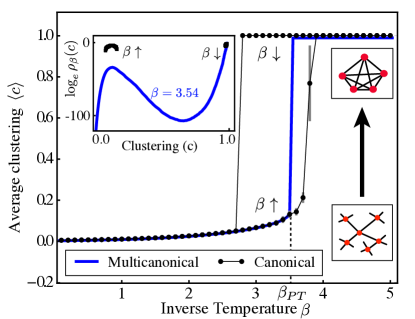
Figure 1: (Color online) Multicanonical sampling of exponential random graphs with imposed clustering avoids the limitations of canonical sampling. The ensemble $\mathcal{G}$ corresponds to k-regular undirected networks with $N=640$ and degree $k=4$. The observable is the clustering coefficient $s=c$ (proportional to the number of triangles, $n_{\triangle}$). The main plot shows $\langle c\rangle$ (and standard deviation) as a function of the inverse temperature $\beta$ obtained by canonical (symbols) and multicanonical (continuous thick line) sampling. Inset: the distribution $\rho_{\beta}(c)$ for $\beta=3.54\approx\beta_{PT}$ obtained by the two methods. Canonical samplings used $5\times 10^{5}$ MCMC steps for equilibration, before another $5\times 10^{5}$ steps were used for estimation. After these steps, the value of $\beta$ was slowly increased ($\beta\uparrow$) or decreased ($\beta\downarrow$) and the process repeated. The multicanonical sampling used $20$ Wang-Landau steps to estimate $\rho_{0}(c)$ (each step used $5$ tunneling steps) Dayal et al. (2004); Landau and Binder (2013).

We are interested in network ensembles that possess one particular observable $s$ of interest, but that are otherwise maximally random. The last requirement is essential to ensure that the ensemble is representative of the networks with a given $s$ and is not subject to additional (hidden) constraints. Both features are achieved by sampling the network from an exponential random graph model (ERGM) Strauss (1986); Snijders (2002); Park and Newman (2004b); Newman (2010); Horvát et al. (2015); Orsini et al. (2015) $\mathcal{G}$, where each graph $g\in\mathcal{G}$ occurs with probability

$$\Pi_{\beta}(g)=\frac{e^{\beta s(g)}}{Z_{\beta}},\text{ where }Z_{\beta}=\sum_{g\in\mathcal{G}}e^{\beta s(g)},$$ (1)

where $s(g)$ is the observable associated with network $g$, and $\beta$ is an inverse-temperature parameter, in analogy to the canonical ensemble in statistical physics. The distribution of $s$ is $\rho_{\beta}(s)=\sum_{g\in\mathcal{G}}\delta(s(g)-s)\Pi_{\beta}(g)=\rho_{0}(s)e^{\beta s}/Z_{\beta}$, where $\rho_{0}(s)\equiv\rho_{\beta=0}(s)$ is called the state density (the fraction of networks $g$ in the ensemble that have observable equal to $s$). The ensemble that acts as a null model for an empirical network with $s=s^{*}$ is usually constructed fixing $\beta$ in such a way that $\langle s\rangle_{\beta}\equiv\sum_{s}s\rho_{\beta}(s)$ equals $s^{*}$. The number of networks in this ensemble typically grows exponentially with the number of nodes, and, thus, besides a small set of observables $s$ that can be treated analytically, investigation of ERGMs requires sampling networks $g$ from $\mathcal{G}$ using Monte Carlo methods Park and Newman (2004b).

The usual approach of sampling from $\mathcal{G}$ is via Markov chain Monte Carlo (MCMC) method works as follows: starting from one network $g\in\mathcal{G}$, a new network $g^{\prime}\in\mathcal{G}_{n}$ is proposed by choosing two links at random and exchanging one of the nodes of each link, which preserves the degree-sequence of the network Maslov and Sneppen (2002). The proposed network is accepted with the Metropolis-Hastings probability $A(g\mapsto g^{\prime})=\min\{1,e^{\beta(s(g^{\prime})-s(g))}\}$ and the process is repeated from $g^{\prime}$ ($g$) if the proposal is accepted (rejected) Newman and Barkema (2002). Since the moves fulfill ergodicity and detailed balance, for sufficiently long times the values of $s$ in the sampled networks $g$ are distributed as $\rho_{\beta}(s)$. However, despite this asymptotic guarantee, in practice this method often fails because the time to approximate $\rho_{\beta}(s)$ grows exponentially with the number of nodes $N$. This happens whenever $\rho_{\beta}$ possesses more than one local maximum (minimum of the free energy) and the barriers between them grow with $N$. As we show below, this generically happens when the observables $s$ are related to motifs.

As an alternative to the canonical (simple Metropolis) sampling method described above, we propose a multicanonical sampling to overcome the aforementioned problem. This method aims to sample networks uniformly on a pre-defined observable range $[s_{min},s_{max}]$, thus overcoming the minima of $\rho_{\beta}(s)$ that are responsible for the weak performance of the canonical method. This is done by sampling the states according to auxiliary ensemble with probabilities $\Pi^{\prime}(g)\propto 1/\rho_{0}(s(g))$, achieved by simply changing the acceptance to $A(g\mapsto g^{\prime})=\min\{1,\rho_{0}(s(g^{\prime}))/\rho_{0}(s(g))\}$ Landau and Binder (2013). However, in order to perform this sampling we need to know the state density $\rho_{0}(s)$. In order to estimate it, we use the Wang-Landau algorithm Wang and Landau (2001); Landau and Binder (2013), which, in short, constructs an adaptive histogram to approximate $\rho_{0}(s(g))$ Note (1). After convergence, $\rho_{\beta}(s)$ is estimated for all $\beta$’s reweighting $\rho_{0}(s)$ through $\rho_{\beta}(s)=\rho_{0}(s)\exp(-\beta s)/Z_{\beta}$ Landau and Binder (2013). Hence, the auxiliary ensemble allows to explore the original canonical ensembles without being restricted to the most probable regions. More importantly, we can impose the desired value of the observable as a hard constraint a posteriori, i.e., only sample networks with $s(g)=s^{*}$. The multicanonical approach has recently been applied to investigate the spectral gap of networks Saito and Iba (2011), and related approaches have been used to investigate percolation Hartmann (2011) and resilience properties of networks Dewenter and Hartmann (2015).

In Fig. 1 we show how the application of multicanonical sampling solves the limitations of canonical sampling in the classical problem of introducing clustering in a $k$-regular network Strauss (1975); Foster et al. (2010). Here, nodes are forced to have the same degree $k$ and the observable of interest is the number of triangles, $s(g)=n_{\triangle}$. Fixing $n_{\triangle}$ is the same as fixing the clustering coefficient $c=3n_{\triangle}/n_{\wedge}$, where $n_{\wedge}$ is the number of connected triples (a constant for all networks with the same degree sequence) Newman (2010). This model exhibits a transition at a specific value of $\beta=\beta_{PT}$ ($\approx 3.54$ for $k=4$), separating low and high-clustering phases Foster et al. (2010). The canonical sampling is unable to compute $\langle c\rangle$ close to the phase-transition because it yields different estimations of $\langle c\rangle$, depending whether $\beta$ is slowly increased ($\beta\uparrow$, lower branch) or decreased ($\beta\downarrow$, upper branch). This hysteresis is typical around first-order phase transitions (coexisting phases) and indicates that the canonical sampling is in a metastable state. Indeed, $\rho_{\beta_{PT}}(c)$ has two local maxima in which the canonical sampling becomes trapped (inset in Fig. 1). On the other hand, the multicanonical sampling is immune to these problems: it correctly characterizes $\langle c\rangle$ at $\beta=\beta_{PT}$ and reveals the full distribution $\rho_{\beta=\beta_{PT}}$. Hence, the method is not only capable of computing the correct ensemble average for any $\beta$, it yields typical networks with any value of $c$, including the significant gap $c\in[.2,1]$ which is unattainable with the canonical sampling. In Fig. 2 we confirm that the computational cost of the multicanonical method scales polynomially with system size, a dramatic improvement over the exponential scaling of the canonical method.

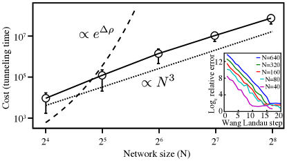
Figure 2: (Color online) Efficiency of the multicanonical method to sample networks with constraints. The computational cost (in number of MCMC steps) to generate an independent realization of a network in the $k$-regular ensemble with $k=3$ is plotted as a function of $N$. In the canonical method close to the critical $\beta$, this requires passing the minimum of $\rho_{\beta}(c)$ (inset of Fig. 1). We measured that the height of this barrier increases as $\Delta\rho\approx 0.4N$, which leads to an exponential increase in the cost (dashed line). Sampling independent realizations in the multicanonical method requires, at most, a tunneling (the number of MCMC steps to do $c=0\mapsto c=1\mapsto c=0$) Dayal et al. (2004). The measured tunneling time (circles and full line) scales polynomially. Inset: convergence of the relative error in the logarithm of the density of states (entropy) during convergence of the Wang-Landau algorithm, estimated comparing the measured value with the exact value on c=1. The saturation of the error observed for large number of steps does not hinder the sampling of any $c$ (see Ref. Belardinelli et al. (2008) for methods to overcome the saturation).

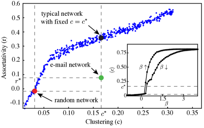
Figure 3: (Color online) Relationship between clustering $c$ and assortativity $r$ in the email network of Ref. Guimerà et al. (2003). The assortativity $r^{*}$ is higher than in a random network with the same degree sequence, but lower than in a typical network with a fixed clustering $c^{*}$. The plot shows $r$ and $c$ of different networks: the email network (green), a typical fully random network (red), a typical random network with $c=c^{*}$ (black), and networks sampled using the multicanonical method from an ensemble with equal probability for networks with the same $c$ (blue dots). Inset: $\langle c\rangle$ obtained using the canonical method.

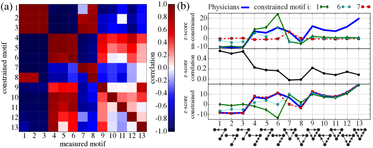
Figure 4: (Color online) Motifs are correlated to each other in blocks. (a) The Pearson correlation coefficient [$R_{ij}=(\langle n_{i}n_{j}\rangle-\langle n_{i}\rangle\langle n_{j}\rangle)/\sigma_{n_{i}}\sigma_{n_{j}}$] between motifs $i$ and $j$, computed by varying the constrained motif (in a range which includes the values of the real and random networks seem SM ). (b) Upper panel: Motif profile Milo et al. (2004) built from the z-score $z_{j}$ vs. $j$ ($z_{j}=(n_{j}-\langle n_{j}\rangle)/\sigma_{n_{j}}$, where $n_{j}$ is the number of motifs $j$ and $\langle\ldots\rangle$ and $\sigma_{j}$ are the average and standard deviation in the $\beta=0$ ensemble). Different lines correspond to the $z_{j}$ of the real network ($z_{j}^{*}$, blue line) and the expected $z_{j}$’s in the constrained ensemble in which $n_{i}$ is equal to the $n^{*}_{i}$ of the real network, where $i$ is the constrained motif shown in the legend ($z_{j}=z_{j}^{*}$ for $j=i$). Middle panel: the correlation between the profiles shown in the upper panel, i.e., between the profile $z$ of the real network and the profile $z^{\prime}$ of the motif-$i$ constrained network (as a function of $i$), computed as $R_{zz^{\prime}}=(\langle zz^{\prime}\rangle-\langle z\rangle\langle z^{\prime}\rangle)/\sigma^{2}_{z}$, where $\langle\ldots\rangle$ and $\sigma_{z}$ were computed over $j\neq i$. Lower panel: comparison of the z-score shown in the upper panel (blue line) and the alternative z-score obtained computing $\langle\ldots\rangle$ and $\sigma_{j}$ in the ensemble constrained by $n_{i}=n_{i}^{*}$, where $i$ is indicated in the legend ($z_{j}\equiv 0$ for $j=i$).

Next we use the multicanonical method to investigate two important problems of social networks. The first problem we consider is to distinguish between homophily (the tendency of “similar” nodes to connect to each other) and transitivity (the tendency of nodes that already share a common neighbor to connect to each other) in social networks Rapoport (1953); Granovetter (1973); Holme and Zhao (2007); Kossinets and Watts (2009); Foster et al. (2011); Bianconi et al. (2014). We use the (undirected) network of email exchange within a university Guimerà et al. (2003). It consists of $N=1,133$ users, and $M=5,451$ email exchanges, and a roughly exponential degree distribution. As observables we consider the clustering coefficient $c$ and the degree assortativity $r$ Newman (2002), for which we obtain $c^{*}=0.166(12)$ and $r^{*}=0.08(3)$ (uncertainties in the last digit estimated using the order-10 Jackknife method). We assess the significance of these values by comparing them to those obtained in the following three network ensembles with the same degree sequence as in the original network:
(i) Same weight to all networks $g$ (i.e. the configuration model). Canonical sampling with $\beta=0$ yields $\langle c\rangle_{\beta=0}=0.028(1)$ and $\langle r_{\beta=0}\rangle=-0.017(13)$, much smaller than $c^{*}$ and $r^{*}$ as typically found in social networks.
(ii) ERGMs with $\langle c\rangle=c^{*}$. In order to determine whether the assortativity is a consequence of high clustering Foster et al. (2011) we would like to measure $\langle r\rangle$ from the null model with $\langle c\rangle=c^{*}$. This canonical sampling fails because $\langle c\rangle_{\beta}$ vs. $\beta$ shows an hysteresis around $s=c^{*}$ (inset of Fig. 2, in agreement with our previous discussion).
(iii) Hard constraints with $c(g)=c^{*}$, obtained using multicanonical sampling. As mentioned before, this type of hard constraint is unfeasible with canonical sampling, even if the desired observable value is realizable. With the multicanonical method we sample points after a number of Monte Carlo steps proportional to the tunneling time, which guarantees that the sampled points are independent and unbiased Dayal et al. (2004). We performed multicanonical sampling for a desired $c$ and measured the assortativity $r$. The results are shown in Fig. 3 and reveal that random networks with the same clustering of the email network $c=c^{*}$ typically show a much larger assortativity $\langle r\rangle>r^{*}$. Therefore, although both $c^{*}$ and $r^{*}$ are larger than one would expect for a fully random network, the actual value of $r^{*}$ is significantly less than one would expect by knowing only $c^{*}$. From this we conclude that the degree homophily is not explained alone by transitivity.

The second problem we address is the extent to which the occurrence of different motifs (connected subgraphs) are related to each other and the impact of such correlations on the so-called motif profiles Milo et al. (2004). Here we focus on directed networks, and the observable of interest is the number $n_{i}$ of occurrences of a specific motif $i$. Again, traditional sampling methods are not suited to address this problem because of the existence of (potentially multiple Foster et al. (2010)) discontinuous phase transitions. Instead, using the multicanonical method, we reliably sample networks with a prescribed count of one particular motif. By measuring the counts of all other motifs, we obtain the correlations between them and the constrained motif. In this manner, we obtain SM the interdependence between all 13 different 3-node motifs in a directed acquaintance network between physicians Coleman et al. (1957) (with $N=241$ nodes and $M=1,098$ edges). The results in Fig. 4 reveal strong positive and negative correlations between pairs of motifs. Two blocks of motifs can be identified ($1,2,3,7,8$ and $4,5,6$, Fig. 4a). Motifs show positive correlations within their blocks and are anti-correlated with motifs in the other blocks (the motifs $9$ to $13$ show a mixed behavior). Given that one motif is over (under) represented, one should expect also an over representation in motifs positively (negatively) correlated with it. As a consequence of this correlation, we find that single motifs explain up to $60\%$ of the variance of the motif profile across the other 12 motifs (Fig. 4b, upper and middle panel). Furthermore, if the constrained ensembles are used to compute alternative $z$-scores, we find that the resulting motif profiles vary dramatically depending on the constraint, with some motifs $j$ showing variations from $z_{j}\gg 0$ to $z_{j}\ll 0$ (Fig. 4b, lower panel). This sensitivity of the motif profile $z_{j}$ shows that such profiles bring limited insights on the over- or under-representation of individual motifs in a network. In particular, since such non-trivial profiles as those seen in Fig. 4b can be obtained by imposing the occurrence of a single motif, it is questionable whether conclusions regarding the underlying formation mechanisms can be reliably reached from them Milo et al. (2004); Artzy-Randrup et al. (2004). Nevertheless, the null models considered here represent a principled approach of assessing the relative significance of motif occurrences that is more meaningful than the usual comparison to fully random networks.

In summary, we have shown that multicanonical sampling allows for an improved network generation and for the investigation of problems which were otherwise intractable. In particular, we characterize ERGMs in cases where the usual canonical sampling fails and we sample networks imposing hard constraints, an alternative to a direct sampling of ERGMs even when the usual algorithms are feasible. Our analysis of empirical networks demonstrates that using the multicanonical sampling allows the investigation of the interdependence between network properties. In particular, we quantified the correlation between clustering and assortativity, and between different motifs, as well as the extent to which their significance profiles can be explained by single motifs. This opens the possibility of investigating the correlation between motifs as well as other local-scale properties and the large-scale structure of networks Foster et al. (2011), such as communities, core-peripheries and many others. The systematic disentangling of these diverse features is a crucial and open problem in the identification of fundamental models of network formation.

Acknowledgments We thank J. M. V. P. Lopes for insightful discussions. This work was partially funded by the University of Bremen, under the program ZF04, and FCT (Portugal), grant SFRH/BD/90050/2012.

Supplemental Material

Wang-Landau algorithm to sample networks

The sampling algorithms used in the paper perform random walks in the space of constrained networks. In our case, this space is built by networks with a fixed number of nodes and a fixed degree sequence (e.g. the degree sequence of the e-mail network). Besides this space, the observable we are interested in characterizing $s(g)$ (e.g. number of triangles of the network $g$) and its range of interest $[s_{\min},s_{\max}]$ are also chosen a priori.

The Wang-Landau algorithm performs a random walk in the space of constrained networks that aims to visit equally often any value of $s\in[s_{\min},s_{\max}]$. The outputs of this algorithm are: 1. a numerical approximation of the state density $\rho_{0}(s)$; and 2. a set of random networks $g$ such that their observables $s(g)$ are uniformly distributed in $[s_{\min},s_{\max}]$. Below we describe the main steps of the Wang-Landau algorithm.

The following quantities have to be initialized and evolve in time:

• a network $g$, initially set to be an arbitrary network with $s(g)\in[s_{\min},s_{\max}]$; $s=s(g)$ represents its observable.

• a histogram-like list $S(s)$, for $s\in[s_{\min},s_{\max}]$ (binned if $s$ is continuous), that represents a discrete approximation of $\log\rho(s)$; it is initialized for all $s$ to $S(s)=0$.

• the Wang-Landau refinement parameter $f$, initialized at $f=1$ (the minimum value $f_{\min}$ is set a priori, e.g. $f_{\min}=2^{-12}$).

The algorithm evolves according to the following rules:

1. Repeat until a pre-defined number (e.g., 10) of round-trips are achieved:

   1. Randomly propose a new network $g^{\prime}$ in the space of constrained networks, and compute $s^{\prime}=s(g^{\prime})$ (see how below);

   2. Update $g,s$ to $g=g^{\prime},s=s^{\prime}$ if $\log(r)<a(s^{\prime},s)=S(s^{\prime})-S(s)$ where $r$ is a random number drawn from a uniform distributed in $[0,1]$;

   3. Update $S(s)=S(s)+f$.

2. update $f$ to $f=f/2$, go to 1. if $f\geq f_{\min}$.

After the convergence of the evolution $(f<f_{\min})$ described above, $S(s)$ is an approximation of $\log\rho(s)$ up to a normalization constant. Setting $f=0$ at this point and repeating loop 1 generates networks $g$ such that $s(g)$ is uniformly distributed in $[s_{\min},s_{\max}]$ (multicanonical ensemble).

Notes:

• A round-trip is achieved in step 1. when, for the first time, the observable went from $s=s_{\min}$ to $s=s_{\max}$ and returned back.

• The network $g^{\prime}$ is constructed by selecting two edges of the original network $g$ and exchanging one of the nodes of one edge by one of the nodes of the other edge. This guarantees that the degree sequence is preserved. For more complicated constraints on which this procedure is not feasible, one can reject a proposed $g^{\prime}$ if it is not in the space of constrained networks.

• In order to achieve a faster computation of $s^{\prime}=s(g^{\prime})$ in 1(a) it is useful to store which motifs any given edge belongs to. Then, instead of re-computing all motifs of $g^{\prime}$ to compute $s^{\prime}=s(g^{\prime})$, one can calculate $s^{\prime}$ from the number of motifs destroyed and created when passing from $g$ to $g^{\prime}$ using the procedure described in the note [ii)].

• A canonic ensemble with fixed $\beta$ is obtained by running loop 1. with $a(s^{\prime},s)=-\beta(s^{\prime}-s)$.

For a more formal description of the Wang-Landau algorithm and for further details we refer to Refs. Wang and Landau (2001); Landau and Binder (2013). In Ref. Note (1) we provide an implementation of the algorithm described above for the case of triangles in undirected networks.

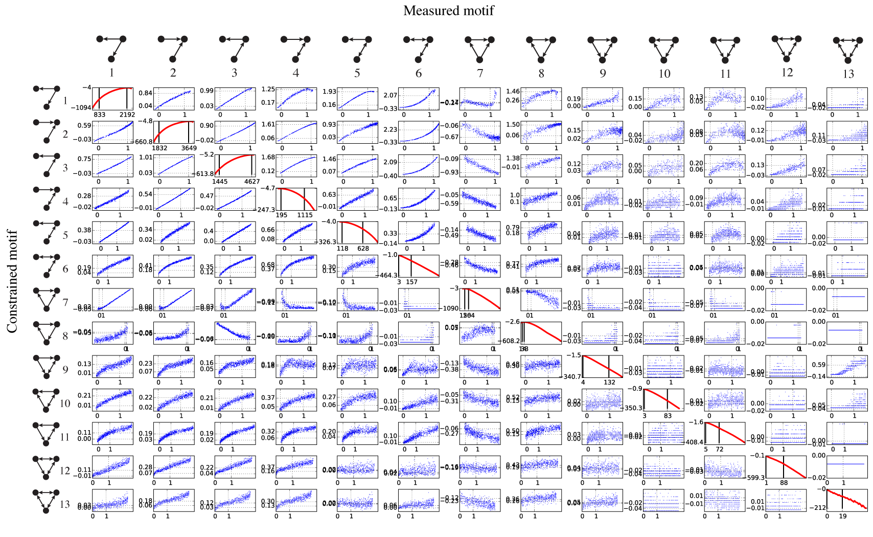
Figure 5: (Color online) Co-dependence between motifs in a directed social network (Physicians). The diagonal plots ($i=j$) show the probability of observing the motif $i$ in the ensemble of random networks with the same degree distribution (state density). Vertical lines indicate the expected number of motifs (close to the maximum) and the number observed in the real network. The non-diagonal plots show the number of motifs $n_{i}$ and $n_{j}$ in random networks with fixed number of $n_{i}$ (constrained motif). For each constrained motif $i$, a multicanonical sampling was performed in the range shown in the plot. For each value of the motif $i$ (vertical axis) in this range, independent samples of networks were recorded and the number of the unconstrained motifs $j$ (horizontal axis) was measured. The (Pearson) correlation between these values is shown in Fig. 4(a). The motif-profile in Fig. 4(b) was obtained over the values of motifs $j$ obtained fixing motif $i$ to the value of the real network.

References

- Nunes Amaral and Guimera (2006) L. A. Nunes Amaral and R. Guimera, Nature Physics 2, 75 (2006).
- Holme and Zhao (2007) P. Holme and J. Zhao, Physical Review E 75, 046111 (2007).
- Newman (2010) M. Newman, Networks: An Introduction (Oxford University Press, 2010).
- Newman et al. (2001) M. E. J. Newman, S. H. Strogatz, and D. J. Watts, Physical Review E 64, 026118 (2001).
- Chung and Lu (2002) F. Chung and L. Lu, Annals of Combinatorics 6, 125 (2002).
- Holland et al. (1983) P. W. Holland, K. B. Laskey, and S. Leinhardt, Social Networks 5, 109 (1983).
- Karrer and Newman (2011) B. Karrer and M. E. J. Newman, Physical Review E 83, 016107 (2011).
- Blitzstein and Diaconis (2010) J. Blitzstein and P. Diaconis, Internet Math. 6, 489 (2010).
- Kim et al. (2012) H. Kim, C. I. D. Genio, K. E. Bassler, and Z. Toroczkai, New Journal of Physics 14, 023012 (2012).
- Orsini et al. (2015) C. Orsini, M. M. Dankulov, A. Jamakovic, P. Mahadevan, P. Colomer-de Simón, A. Vahdat, K. E. Bassler, Z. Toroczkai, M. Boguñá, G. Caldarelli, S. Fortunato, and D. Krioukov, (2015), arXiv:1505.07503 (to appear in Nature Communications) .
- Strauss (1975) D. J. Strauss, Biometrika 62, 467 (1975).
- Park and Newman (2004a) J. Park and M. E. J. Newman, Physical Review E 70, 066146 (2004a).
- Foster et al. (2010) D. Foster, J. Foster, M. Paczuski, and P. Grassberger, Physical Review E 81, 046115 (2010).
- Foster et al. (2011) D. V. Foster, J. G. Foster, P. Grassberger, and M. Paczuski, Physical Review E 84, 066117 (2011).
- Beber et al. (2012) M. E. Beber, C. Fretter, S. Jain, N. Sonnenschein, M. Müller-Hannemann, and M.-T. Hütt, Journal of the Royal Society Interface 9, 3426 (2012).
- Milo et al. (2002) R. Milo, S. Shen-Orr, S. Itzkovitz, N. Kashtan, D. Chklovskii, and U. Alon, Science (New York, N.Y.) 298, 824 (2002).
- Milo et al. (2004) R. Milo, S. Itzkovitz, N. Kashtan, R. Levitt, S. Shen-Orr, I. Ayzenshtat, M. Sheffer, and U. Alon, Science (New York, N.Y.) 303, 1538 (2004).
- Artzy-Randrup et al. (2004) Y. Artzy-Randrup, S. J. Fleishman, N. Ben-Tal, and L. Stone, Science (New York, N.Y.) 305, 1107 (2004).
- Ugander et al. (2013) J. Ugander, L. Backstrom, and J. Kleinberg, in Proceedings of the 22Nd International Conference on World Wide Web, WWW ’13 (2013) pp. 1307–1318.
- Landau and Binder (2013) D. Landau and K. Binder, A guide to Monte Carlo simulations in statistical physics (Cambridge University Press, 2013).
- Dayal et al. (2004) P. Dayal, S. Trebst, S. Wessel, D. Wurtz, M. Troyer, S. Sabhapandit, and S. N. Coppersmith, Physical Review Letters 92, 097201 (2004).
- Strauss (1986) D. Strauss, SIAM Review 28, 513 (1986).
- Snijders (2002) T. A. Snijders, Journal of Social Structure 3, 40 (2002).
- Park and Newman (2004b) J. Park and M. E. J. Newman, Physical Review E 70, 066117 (2004b).
- Horvát et al. (2015) S. Horvát, E. Czabarka, and Z. Toroczkai, Physical Review Letters 114, 158701 (2015).
- Maslov and Sneppen (2002) S. Maslov and K. Sneppen, Science (New York, N.Y.) 296, 910 (2002).
- Newman and Barkema (2002) M. E. J. Newman and G. T. Barkema, Monte Carlo Methods in Statistical Physics (Oxford University Press, USA, New York, 2002).
- Wang and Landau (2001) F. Wang and D. P. Landau, Physical Review Letters 86, 2050 (2001).
- Note (1) We describe the multicanonical sampling method proposed in this Letter in the Supplemental Material and we provide an implementation at https://dx.doi.org/10.5281/zenodo.30626.
- Saito and Iba (2011) N. Saito and Y. Iba, Computer Physics Communications 182, 223 (2011).
- Hartmann (2011) A. K. Hartmann, The European Physical Journal B 84, 627 (2011).
- Dewenter and Hartmann (2015) T. Dewenter and A. K. Hartmann, New Journal of Physics 17, 015005 (2015).
- Belardinelli et al. (2008) R. E. Belardinelli, S. Manzi, and V. D. Pereyra, Physical Review E 78, 067701 (2008).
- Guimerà et al. (2003) R. Guimerà, L. Danon, A. Díaz-Guilera, F. Giralt, and A. Arenas, Physical Review E 68, 065103 (2003).
- Rapoport (1953) A. Rapoport, The Bulletin of Mathematical Biophysics 15, 523 (1953).
- Granovetter (1973) M. S. Granovetter, American Journal of Sociology 78, 1360 (1973).
- Kossinets and Watts (2009) G. Kossinets and D. J. Watts, American Journal of Sociology 115, 405 (2009).
- Bianconi et al. (2014) G. Bianconi, R. K. Darst, J. Iacovacci, and S. Fortunato, Physical Review E 90, 042806 (2014).
- Newman (2002) M. E. J. Newman, Physical Review Letters 89, 208701 (2002).
- Coleman et al. (1957) J. Coleman, E. Katz, and H. Menzel, Sociometry 20, 253 (1957).
- (41) Fig. 5 below. .

References

- Wang and Landau (2001) F. Wang and D. P. Landau, Physical Review Letters 86, 2050 (2001).
- Landau and Binder (2013) D. Landau and K. Binder, A guide to Monte Carlo simulations in statistical physics (Cambridge University Press, 2013).
- Note (1) A C++ code demonstrating the usage of Monte Carlo flat-histogram to sample constrained networks, https://dx.doi.org/10.5281/zenodo.30626.