Enhanced Casimir effect for doped graphene
Abstract
We analyze the Casimir interaction of doped graphene. To this end we derive a simple expression for the finite temperature polarization tensor with a chemical potential. It is found that doping leads to a strong enhancement of the Casimir force reaching almost in quite realistic situations. This result should be important for planning and interpreting the Casimir measurements, especially taking into account that the Casimir interaction of undoped graphene is rather weak.
Introduction
Graphene, which is a two-dimensional sheet of carbon atoms possesses many unusual properties and attracts a lot of attention. Particular excitement among the theoreticians is caused by the fact that the spectrum of quasi-particles in graphene is described by the quasi-relativistic Dirac model with the effective propagation speed of about 300 times less than the speed of light. This continuous model turned out to be very successful in describing a broad range of effects Katsnelson , for instance optical properties of graphene as the absorption of light abs and the (giant) Faraday effect Faraday , to mention a few.
In the recent years, the Casimir effect for pristine graphene was studied both for zero Bordag:2009fz ; DW and finite Dobson ; Gomez ; Fialkovsky:2011pu temperatures. For not too large temperatures (as compared with inverse distance between the interaction sheets) the effect between graphene monolayer and ideal metal is defined by the fine structure constant and is roughly of the one between two ideal metal plates. Such small forces are on the limit of sensitivity of modern experimental techniques. For high temperatures (or separations) the effect is hugely reinforced Fialkovsky:2011pu , but the measurements under such conditions is a separate quite challenging task, which is not completely solved yet even for metals, see e.g. Mostepanenko15 . It is not surprising therefore that just a single experiment has been performed until now graCas-exp . This experiment revealed graCas-compar a good agreement with the theory Bordag:2012hi . Possibilities, opened by doping, were however not explored there.
Previously the Casimir interaction of doped graphene was studied in Bo ; Sara . The reflection coefficients used in that works were expressed though quantities whose explicit dependence on the temperature remained unknown and the results of Refs. Bo ; Sara are mutually contradicting. Therefore, specifically after experimental confirmation of the Dirac approach to Casimir energy of undoped graphene graCas-exp ; graCas-compar , it seems to be important to extend the approach to doped graphene.
In this letter we consider the Casimir effect at finite temperature, chemical potential and mass, and find a substantial enhancement of the effect in graphene-metal systems which potentially permits to avoid the above mentioned experimental difficulties. Our findings show that for relatively highly (but still feasibly) doped graphene monolayers the effect gets stronger by approximately . In the (formal) limit of an infinite chemical potential the Casimir interaction becomes of that for the ideal metal. Our calculation is based on a complete representation of the polarization tensor of the fermionic quasi-particles in graphene at finite temperature, chemical potential and mass gap. The obtained result is surprisingly simple and can be easily analytically continued to whole complex frequency plane, including, importantly, real optical frequencies. It is based on the QED formalism applied to graphene-like systems in Gusynin ; Pyatkovskiy , and generalizes the results of Bordag:2009fz ; Fialkovsky:2011pu ; Bordag:2015gla and those of Bordag:2015 , which also allows continuation to the whole plane of complex frequencies, to the case of simultaneous presence of finite chemical potential, finite temperature and non-zero mass-gap. We also describe a very precise approximation scheme that considerably simplifies the computation of Casimir interaction with graphene.
Model
The theoretical description of the electronic properties of graphene based on the continuous Dirac model with a -dimensional action. In the notations of gra-QFT it reads
| (1) |
where and . The gamma matrices are rescaled, . We use natural units , and the Fermi velocity is . Thereby we assume that the graphene monolayer is placed at the plane. The electromagnetic potential is normalized in such a way that .
Reflecting the spin and valley degeneracy in graphene, the gamma matrices, , are being a direct sum of four representations (with two copies of each of the two inequivalent ones). The value of the mass gap parameter and mechanisms of its generation are under discussion Gusynin ; Pyatkovskiy .
As shown in many previous works, see reference in gra-QFT , the electronic properties of graphene in the formalism of Quantum Field Theory (QFT) can be described by the one loop polarization operator, which is gauge invariant in QED-like model defined by 1. In Minkowski momentum space it is given by
| (2) |
where , , and is the causal (Feynman) propagator of the quasiparticles in graphene,
| (3) |
(). Note that due to the quasi-relativistic nature of excitations in graphene also depends on the Fermi velocity . Further notations are , , and is the chemical potential.
Temperature is introduced using the Matsubara formalism. In the -trace in 2, which can be calculated immediately, see e.g. Eq. (A20) in Bordag:2015gla , one has to substitute the integral by a sum,
| (4) |
where is integer. The external frequency of the polarization operator is bosonic, ,
Calculation of the polarization operator for finite temperature, mass gap and chemical potential
All components of the polarization tensor can be expressed via two scalar quantities (form factors), and Zeitlin ; Fialkovsky:2011pu . As in the QED/QCD cases these quantities consist of the vacuum part and a part carrying the dependence on and ,
| (5) |
where stands either for ’’ or ’’. The vacuum part, , corresponds to . While such decomposition is a well known feature of polarization tensor in different theories, see e.g. shuryak , its realization in particular cases and derivation of simple transparent formulas may be a challenging task. One transforms the sum over the Matsubara frequencies 4 into a contour integral consisting of three parts, one of which gives the original integral over the continuous (Euclidean) momenta and the other two can be taken explicitly by the Cauchy theorem. The remaining integral over the in-plane momenta, , can be further simplified by performing the angular integration. Recently such procedure was applied to graphene at , in Bordag:2015 and , in Bordag:2015gla . Omitting the technicalities we arrive at
| (6) | |||
Here the distribution function, , carries the dependence on and . Further notations in 6 are
Note that , 6, does not have UV singularities.
For the vacuum part, , one can directly use the well-known expressions Bordag:2009fz valid for graphene,
| (7) |
where . From now on we set (gapless graphene) unless otherwise stated.
One of the advantages of the decomposition 5 is the absence of the summation over Matsubara frequencies, which permits relatively easy derivation of the limiting cases. In particular, in the limit of zero temperature (but not zero chemical potential) we obtain
| (8) | |||
| (9) | |||
with . The formulae above are the analogue of the (B2) Bordag:2015gla taken at Matsubara frequencies, and one can check that in the appropriate limits they reproduce the results of other authors Bordag:2009fz ; Fialkovsky:2011pu ; Gusynin ; Pyatkovskiy ; Bordag:2015 ; Bordag:2015gla . Similar to the results of Bordag:2015 , the representation 5 with 6 directly permits for continuation to the real frequencies, and thus can be applied for investigation of the optical properties, surface plasmons and other effects in graphene for finite temperature and chemical potential.
Enhancement of the Casimir effect
The Casimir energy density (per unit area) for two parallel interfaces separated by the distance is given by the Lifshitz formula Lifshtz in terms of the reflection coefficients, , , of the TE and TM electromagnetic modes on the two interfaces,
| (10) |
where , and are the Matsubara frequencies 111To restore physical units in Eq. (10) it is enough to apply the conversion rule .. The reflection coefficients are taken at Euclidean momenta . They were derived in Fialkovsky:2011pu in terms of the polarization operator components ,
| (11) |
(and rederived in numerous papers afterwards). For the perfect conductor, . Combining 10 with (11) and using (5,6) for the polarization operator at finite temperature and chemical potential, we are able to calculate the Casimir energy density, , the Casimir pressure , and its’ gradient, , between a doped graphene layer and an ideal metal plate.
It is instructive to consider the case of very large first. In the formal limit , both and have identical asymptotics,
| (12) |
which can be readily deduced from (8,9). Thus the electronic properties of graphene would be expected to become closer to those of ideal metal. However, due to the specific structure of the reflection coefficients 11, it is only the contribution of TM mode to the Casimir interaction which grows in this limit. Thus, at , the Casimir interaction reaches the value of of the ideal metal - ideal metal one,
| (13) |
The same result was obtained for the high temperature limit Fialkovsky:2011pu . Interestingly, the Casimir interaction of graphene can never reach of that for the ideal metal. Eq. (13) gives a very rough idea on how far the enhancement of the Casimir effect with might go. Practically, it hardly makes sense to consider exceeding a couple of eV in the framework of the Dirac model.
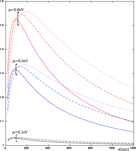
Our numerical analysis show that at distances about – nanometers the Casimir effect between a perfect metal plate and doped graphene is highly enhanced even for relatively moderate values of the chemical potential. On Fig. 1 we compare the behavior of the ratios of the energy, pressure and the pressure gradient at given values of the chemical potential to the corresponding values for pristine graphene, as functions of distance. For eV, the interaction force for the case of doped graphene is only % higher then in the case of pristine graphene. However, already for eV their ratio has a maximum of % at approximately nm, and for eV the force between a doped graphene layer and an ideal metal is almost % higher then that for a pristine one. All our simulations are performed at K and .
One further notices, that the effect is more pronounced the more derivatives we calculate of the energy. Thus, the ratio of the energy at eV to its pristine value is at maximum, for the force it is and for the gradient it reaches . Moreover, at larger distances (– nm), the enhancement effect for the gradient diminishes much slower then that for the energy, which suggests preference for gradient force experiments.
Reaching the values of the chemical potential of eV and higher might be a challenging task and would require preparation of special samples. Without special treatment, the chemical potential in epitaxial graphene layers stays low up to the level of – eV or smaller coletti10 ; riedl10 . However, the Fermi energy shifts of order eV are achievable in epitaxial single layer graphene due to molecular doping Zhou08 . Under certain circumstances, doping may lead to considerable inhomogeneities in the charge distribution, see e.g. inhomo , that may give rise to additional forces in the Casimir experiments. Due to the strong charge density dependence on the nature of acceptor/donor mechanism, these forces should be treated individually for each particular experiment.
The distance dependence of the Casimir energy for doped graphene will be altered as compared to the pristine one as it is usual when an additional dimensionfull parameter is introduced. However, its detailed study is beyond the scope of the present letter.
Influence of the mass gap.
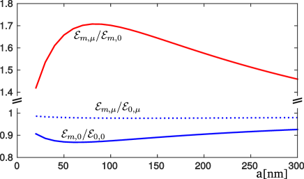
From the physical point of view, the larger is the mass parameter in 1 the less should be the conductivity of quasi-particles and, consequently, the smaller the Casimir effect. This was shown explicitly in Bordag:2009fz for . One can also show that the influence of mass is negligible as far as . In particular, in the formal limit 12 any dependence on the mass disappears. Our numerical simulation shows, see Fig 2, that for eV and eV doping gives up to % enhancement of the Casimir energy density (red line, to be compared with the full red line of Fig. 1). In the same picture it is shown that the influence of the mass gap on the value of the energy for doped graphene (blue dotted line) is almost negligible, while the energy for pristine graphene gets lower by about % (blue full line). Therefore, doping becomes even more important for gaped graphene.
Approximating the Casimir energy.
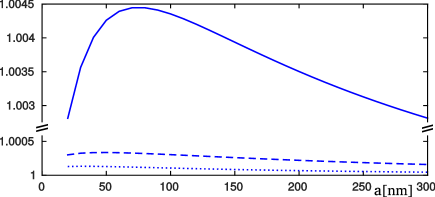
For finite temperature, the numerical calculation of the Casimir energy in a realistic set-up requires summing a large number of contribution to the sum over the Matsubara frequencies. Following the ideas of Fialkovsky:2011pu (which were later confirmed in KM15 ), one might facilitate significantly this calculus by considering the approximation (8,9) for the polarization operator in all terms of the summation 10 except in the zeroth one. The comparison of exact results for the Casimir energy with such approximation, , is given on Fig. 3. As one can see, the error is less then % for the pristine graphene and one order of magnitude smaller for doped one. This confirms once again at an even better level the asymptotic considerations delivered in Fialkovsky:2011pu .
Summary.
In this letter we calculated the polarization operator for the quasi-particles in graphene at non-zero temperature, chemical potential and mass gap applicable at all complex frequencies without a need for any special procedure of analytical continuation. This result can be used in a variety of physical problems, including investigation of TE surface plasmons in graphene Bordag:2015gla , quantum reflection Dufour13 , Casimir interaction, etc.
Basing on these results and the Lifshitz formula, we numerically simulate the Casimir interaction between a doped graphene monolayer and an ideal metal. For high but feasible doping we predict the enhancement of the Casimir effect as compared to the case of the pristine graphene of up to % for the Casimir force, and of up to % — for the force gradient. The high doping of graphene is shown to bring significant enhancement in the values of the force gradient at a wide range of separations which should facilitate future experimental measurements. At such levels of doping the influence of the mass-gap is not important. We saw also that even moderate values of the chemical potential have a non-negligible effect on the Casimir force and thus should be taken into account in realistic description of experiments together with real material properties, finite temperature and mass-gap parameter, if present.
All calculations of the present paper were performed in fully retarded approach valid at all distance. It may be interesting to study whether the non-retarded approach may deliver a good approximation at some distances.
Finally we note, that the considerations given in this letter are concerned with the proper graphene properties and the enhancement of the Casimir interaction is invoked by the change in its conductivity. Thus, we can conclude that even in the experiments involving a real metal and/or graphene on a substrate the enhancement effect must be present, though its particular value may differ from the one presented here. The good concordance between the force gradient measurements graCas-exp and theoretical considerations presented in graCas-compar shows that the graphene samples used in graCas-exp were rather pristine.
Acknowledgments
This work was supported in part by CNPq and FAPESP.
References
- (1) M. I. Katsnelson, Graphene: Carbon in Two Dimensions (Cambridge University Press, Cambridge, England, 2012).
- (2) R. R. Nair et al, Science 320, 1308 (2008).
- (3) I. Grassee et al, Nature Physics 7, 48 (2011), arXiv:1007.5286v1 [cond-mat.mes-hall]; I. V. Fialkovsky and D. V. Vassilevich, Eur. Phys. J. B 85, 384 (2012) [arXiv:1203.4603 [cond-mat.mes-hall]].
- (4) M. Bordag, I. V. Fialkovsky, D. M. Gitman and D. V. Vassilevich, Phys. Rev. B 80, 245406 (2009) [arXiv:0907.3242 [hep-th]].
- (5) D. Drosdoff and L. Woods, Phys. Rev. B 82, 155459 (2010).
- (6) J. F. Dobson, A. White, and A. Rubio, Phys.Rev.Lett.96, 073201 (2006).
- (7) G. Gómez-Santos, Phys.Rev.B 80, 245424 (2009).
- (8) I. V. Fialkovsky, V. N. Marachevsky and D. V. Vassilevich, Phys. Rev. B 84, 035446 (2011) [arXiv:1102.1757 [hep-th]].
- (9) V. M. Mostepanenko J. Phys.: Condens. Matter, 27, 214013 (2015).
- (10) A. A. Banishev, et al., Phys. Rev. B, 87, 205433 (2013)
- (11) G. L. Klimchitskaya, U. Mohideen, V. M. Mostepanenko, Phys. Rev. B, v.89, 115419 (2014)
- (12) M. Bordag, G. L. Klimchitskaya and V. M. Mostepanenko, Phys. Rev. B 86, 165429 (2012) [arXiv:1209.3302 [cond-mat.mtrl-sci]].
- (13) Bo E. Sernelius, Europhys. Lett. 95, 57003 (2011); Phys. Rev. B 85, 195427 (2012).
- (14) J. Sarabadani, A. Naji, R. Asgari and R. Podgornik, Phys. Rev. B 84, 155407 (2011).
- (15) E. V. Gorbar, V. P. Gusynin, V. A. Miransky and I. A. Shovkovy, Phys. Rev. B 66, 045108 (2002) [arXiv:cond-mat/0202422]; V. P. Gusynin and S. G. Sharapov, Phys. Rev. B 73, 245411 (2006) [arXiv:cond-mat/0512157]; V.P. Gusynin, S.G. Sharapov, J.P. Carbotte, New J. Phys. 11, 095013 (2009) [arXiv:0908.2803v2].
- (16) P. K. Pyatkovskiy, J. Phys.: Condens. Matter 21, 025506 (2009).
- (17) M. Bordag and I. G. Pirozhenko, Phys. Rev. D 91, 085038 (2015), arXiv:1502.00421 [cond-mat.mes-hall].
- (18) M. Bordag, G. L. Klimchitskaya, V. M. Mostepanenko, V. M. Petrov Phys. Rev. D 91, 045037 (2015)
- (19) I. V. Fialkovsky, D. V. Vassilevich, Int. J. Mod. Phys. A 27, 1260007 (2012), arXiv:1111.3017v2 [hep-th].
- (20) V. Zeitlin, Phys. Lett. B 352, 422 (1995).
- (21) E. Shuryak, Phys. Rep. 61, 71 (1980).
- (22) E. M. Lifshitz, Zh. Eksp. Teor. Fiz. 29, 94 (1955) [Sov. Phys. JETP 2, 73 (1956)]; E. M. Lifshitz and L. P. Pitaevskii, Statistical Physics: Part 2 (Pergamon Press, Oxford, 1980).
- (23) C. Coletti et al., Phys. Rev. B 81 (2010) 235401.
- (24) C. Riedl et al., J. Phys. D: Appl. Phys. 43, 374009 (2010).
- (25) S. Y. Zhou et al., Phys. Rev. Lett. 101, 086402 (2008), arXiv:0807.4791v2.
- (26) J. Romaneh et al, Nanotechnology 22, 295705 (2011).
- (27) G. L. Klimchitskaya and V. M. Mostepanenko Phys. Rev. B 91 174501 (2015)
- (28) G. Dufour et al., Phys. Rev. A 87, 022506 (2013); Phys. Rev. A 87, 012901 (2013).