Multiple Outlier Detection in Samples with Exponential & Pareto Tails: Redeeming the Inward Approach & Detecting Dragon Kings

Abstract

We consider the detection of multiple outliers in Exponential and Pareto samples – as well as general samples that have approximately Exponential or Pareto tails, thanks to Extreme Value Theory. It is shown that a simple “robust” modification of common test statistics makes inward sequential testing – formerly relegated within the literature since the introduction of outward testing – as powerful as, and potentially less error prone than, outward tests. Moreover, inward testing does not require the complicated type 1 error control of outward tests. A variety of test statistics, employed in both block and sequential tests, are compared for their power and errors, in cases including no outliers, dispersed outliers (the classical slippage alternative), and clustered outliers (a case seldom considered). We advocate a density mixture approach for detecting clustered outliers. Tests are found to be highly sensitive to the correct specification of the main distribution (Exponential/Pareto), exposing high potential for errors in inference. Further, in five case studies – financial crashes, nuclear power generation accidents, stock market returns, epidemic fatalities, and cities within countries – significant outliers are detected and related to the concept of ‘Dragon King’ events, defined as meaningful outliers of unique origin.
Keywords: Outlier Detection, Exponential sample, Pareto sample, Dragon King, Extreme Value Theory

1 Introduction

Much of the outlier testing/detection literature (e.g., [4, 22] are classic references) focuses on testing outliers relative to a main/null model that is Normal. The case of an Exponential null df (distribution function) has also been covered ([2] provides a review). This case, which is considered in the present work, is much more general than typically claimed. For instance, by a simple transformation, the outlier tests in an Exponential sample are applicable to Pareto (power law) samples. Further, Extreme Value Theory (EVT) [13] provides that general “well behaved” untruncated dfs asymptotically have either Exponential or Pareto tails. Thus, this setting is very general.

In addition to the specific contributions of this work, its structure and content differ from standard works on outlier testing in Exponential samples. First, rather than focusing on a single test statistic, with specific null and alternative models, we consider a variety of test statistics, testing procedures, and alternative models. This comprehensive comparison enables the discussion of issues and their solutions that are basic, but fundamental, and – in the opinion of the authors – have not been emphasized in the literature. Second, we shift our focus from reliability applications (the Exponential case) towards applications in risk modeling (the Pareto case). Indeed, Pareto (power law) distributions seem to be ubiquitous in most natural hazards (earthquakes, landslides, mountain collapses, floods, droughts, storms, hurricanes, tsunamis, etc.), industrial catastrophes (chemical spills, nuclear accidents, hydro-electric dam ruptures, power black-outs, Internet outages, traffic grid-locks in highways, congestion in communication networks and so on), social systems and in the geopolitical domain (distribution of wars and conflicts intensities measured by human losses) and so on (see e.g. [37, 38, 48] and references therein). Furthermore, a number of studies have found either strong or, in other cases, suggestive evidence that there are extreme events “beyond” the Pareto sample [49, 53]. This brings into play the concept of “Dragon Kings” (DK) [49], which will be elaborated.

Section 2 presents the general methodology, its justification, and a battery of statistical tests for the detection of outliers. In Section 2.1, the use of Exponential and Pareto outlier tests in the tails of general dfs is justified with EVT. In Section 2.2, a background on outlier detection in Exponential samples is given, including a discussion of masking and swamping errors, and of block and sequential testing procedures. In Section 2.3, a variety of test statistics are summarized, and a robust modification is introduced that minimizes the risk of masking in inward testing. In Section 2.4, the power of block tests for multiple outliers is evaluated, including the case of clustered outliers. A density mixture approach to outlier detection, which is well suited to this case, is also considered. In Section 2.5, the degree to which masking and swamping errors afflict the test statistics is studied. In Section 2.6, the performance of sequential inward, outward, and mixture density procedures is explored in a number of scenarios. In Section 2.7, the sensitivities of the power and level of the tests to misspecification of the null Exponential model are exposed.

In Section 3, the Dragon King (DK) concept is explained and five case studies are presented, which highlight results from previous sections. The case studies are: financial crashes (drawdowns), nuclear power generation accidents, stock returns, fatalities in epidemics, and city sizes. Section 4 concludes with a discussion.

2 Methodology

The setup that we consider is an ordered sample $x_{(1)}>x_{(2)}>...>x_{(n)}$ where $n-k$ of the observations are realizations of a random variable, $X\overset{\text{iid}}{\sim}F_{X}(x)$, with the Exponential df,

$$F_{X}(x)=1-\text{exp}\{-\alpha x\},~{}x\geq 0,~{}\alpha>0~{},$$ (1)

and is abbreviated Exp($\alpha$); and the remaining $k$ are outliers from the contamination df, $Y\overset{\text{iid}}{\sim}F_{Y}$, with $Y$ independent of $X$. We do not know which points are outliers and we want to detect them. A common alternative model is the slippage model where the contamination df $F_{Y}=F_{X}(x/\beta),~{}\beta\geq 1$ is a scale-inflated Exponential df. In this case, the detection problem is the slippage test with $H_{0}:\beta>1$. Much of the literature considers optimality of tests with respect to this alternative.

2.1 Justification for outlier testing relative to Pareto and Exponential tails

It is important to note that outlier tests based on both the Pareto and Exponential dfs are generally applicable to data having approximately Pareto or Exponential tails. This follows from the well known Pickands-Balkema-de Haan theorem of EVT, that states [13]: for a broad range of dfs for random variable X, for sufficiently high threshold $u$, the excess df $F_{u}(x)=P\{X-u\leq x|X-u>0\}$ (i.e., the tail of the df) is approximated by the Generalized Pareto df,

$$GPD(x;\xi,\beta,\mu)=\begin{cases}1-\left(1-\xi(x-\mu)/\beta\right)^{-1/\xi},&\text{if $\xi\neq 0$}\\ 1-\text{exp}(-(x-\mu)/\beta),&\text{if $\xi=0$ },\end{cases}$$ (2)

in the sense that,

$$\text{lim}_{u\rightarrow\infty}\text{sup}_{0\leq x}\left|~{}F_{u}(x)-GPD\left(x|\xi,\beta(u),\mu\right)\right|=0~{},~{}~{}~{}\beta(u)>0,\forall u.$$ (3)

Where $\xi=0$ (the Gumbel case), the GPD (2) is the Exponential df with lower truncation $\mu=u$ and scale parameter $\beta=1/\alpha$. This case includes common dfs such as the Exponential (obviously), the Normal, and even some fat-tailed dfs such as the Lognormal. Where $\xi>0$ (the Fréchet case), the GPD (2) is Pareto with $\mu=u$, $\sigma=u/\alpha$, and $\xi=1/\alpha$. This case includes heavy tailed dfs such as the Pareto, Burr, and Log-gamma. The only other case ($\xi<0$: the Weibull case) is where the df has a finite upper endpoint, and thus this case is of less interest in outlier detection. Therefore outlier testing in Exponential and Pareto samples is (asymptotically) extremely general!

Since the GPD approximation (3) is asymptotically valid – and the rate of convergence depends on the unknown underlying df [13] – one must select a sufficiently large lower threshold $u$ before applying the outlier tests. For instance, in the Pareto case, in practice it is typical that the body of the empirical CCDF is sub-linear in log-log scale, and only becomes linear in the tail, whereas the Pareto is linear for its entire support. Here, if $u$ is too small, then the estimated tail will be too heavy – effectively masking outliers and weakening the test. For growing $u$, the test will become increasingly powerful.

When estimating the GPD (3) in practice, increasingly large lower truncations $u$ are considered, and the parameter estimates are taken at the smallest $u$ above which parameter estimates are stable. This procedure is typically represented in the well known Hill plot. For outlier testing, we propose a similar approach. For instance, in addition to requiring that the null model fits the non-outlying portion of the sample, the test should be applied for the top ten through top hundred points, and consistent rejection in the upper most subsamples, where (3) is most relevant, should be interpreted as a rejection. This involves multiple dependent tests. One can frequently reject the null if the smallest p-value is selected from a long sequence of such tests. However, under the null, where tests are done for $n$ upper points, $n-1$ upper points, etc., the probability of rejecting $c=1,2,3,\dots$ consecutive tests decreases with growing $c$. Based on simulation studies with the range of models considered within this work, we offer as a rough rule of thumb that for a sample of size $10<n<100$, one should require a run of $c=n/10$ tests to be rejected to maintain control of the type 1 error. This approach is applied in the case studies (Sec. 3).

2.2 Background: masking vs swamping and inward vs outward tests

For a statistical outlier test, one not only wants to have high power and computational tractability, but also to estimate the number of outliers $k$ well. Masking and swamping errors are impediments to this task.

• For $k$ actual outliers, and $r$ hypothesized outliers, with $r<k$, a first outlier masks a second if the second outlier is only identified as an outlier when the first is not present. That is, considering $r<k$ outliers, $k-r$ outliers have been left in the sample, and may skew the statistics enough so that the $r$ hypothesized outliers do not appear very extreme. The larger the $k-r$ outliers remaining in the sample, the worse the masking.

  To quote the classic text [22] on masking: “This effect occurs quite generally- as a class, the statistics that are effective in identifying a single outlier tend to lose power badly if more than one outlier is present.”, and,
  “It must be supposed that the prevalence and potential seriousness of the masking effect is the main cause, both of the large degree of attention given in the literature to the detection of multiple outliers, and the fact that none of the solutions proposed is entirely satisfactory.”

• For $k$ actual outliers, and $r$ hypothesized outliers, with $r>k$, an outlier swamps a non-outlier when the non-outlier is only identified as an outlier when considered in the presense of the outlier. That is, when $r-k$ non-outliers are grouped with the $k$ outliers within a test statistic, the test may still reject the null hypothesis, especially if the outliers are large. This error is of secondary concern relative to masking, which prevents the discovery of any result.

A simple approach to detecting outliers is a block test, where the number of outliers, $r$, is specified a-priori and, in a single test, either r or 0 outliers are identified. That this procedure suffers from masking and swamping, when too many or too few points are included in the block respectively, is both clear and well documented. However, if well specified, block tests are powerful due to the simultaneous usage of all data. To avoid dependence on the specification of block size $r$, sequential tests were developed:

• One starts with the full sample and tests if the largest point is outlying. If that point is identified as outlying (the test is rejected), then it is removed from the sample and the test is repeated with the next largest point. The procedure is repeated until the first failure to reject. The estimated number of outliers $\widehat{k}$ is the number of rejected (marginal) tests. Clearly, this test can suffer from both masking and swamping. The weaknesses of the inward procedure were cited as motivation for the outward test [43, 22, 27]:

• One specifies a maximum number of outliers $r$, and starts by testing if the $r$th largest point $x_{(r)}$ is an outlier by deleting the other $r-1$ largest values $x_{(r-1)},x_{(r-2)},...,x_{(2)},x_{(1)}$ and applying the test on $x_{(r)}$. If this test is rejected, then $r$ outliers are identified. If this test is not rejected, then one takes a step “outward”, which involves then testing the $(r-1)$th largest point $x_{(r-1)}$. This testing of increasingly large points is done until the first rejected test, say for $x_{(j)},~{}j\in\{1,...,r\}$, thus identifying $\widehat{k}=j$ outliers. If none of the tests are rejected, then no outliers are identified. This test minimizes the probability and magnitude of both masking and swamping. As such, the outward procedure has been claimed superior over the inward [27, 7, 3] and received more subsequent development [33, 34].

However, control of the type 1 error (the probability of a false alarm) is difficult in the outward test. The test considers the null hypothesis $H_{0}$ that there are no outliers, with multiple alternatives, $H_{j},~{}j=1,...,r$ that there are $j$ outliers, with test statistics $T_{j}$. A single rejection of the $r$ tests rejects the null $H_{0}$. Thus, to achieve an overall type 1 error level of $0\leq a\leq 1$, the marginal tests need to have a lower level. And, the larger $r$, the more power the test loses. This “multiple testing correction” requires knowing the joint df of, generally dependent, $T_{j},~{}j=1,...,r$ (and also the marginal dfs)! More specifically, one defines all marginal tests to have equal level $b$, i.e., $Pr\{T_{j}>t_{j}\}=b,~{}j=1,...,r$, and the level $b$ is determined such that $Pr\{T_{j}\leq t_{j},~{}j=1,...,r|H_{0}\}=1-a$. Clearly $a^{r}\leq b\leq a$, where the lower bound corresponds to the case of independent tests (the Bonferonni bound), and the upper bound to perfect dependence. For the specific test statistic (6) discussed below, the joint and marginal dfs were derived for $k=2,3$ in [27], and a Monte-Carlo implementation recommended in [33] for larger $k$.

In contrast, for the inward method, the type 1 error level is equal to the marginal level ($a=b$). This is because a rejection of the null only happens when the first marginal test (for the largest point, $x_{(1)}$) is rejected. This is a major advantage over the outward procedure in terms of computation and also because no power is lost due to a multiple testing correction.

2.3 Gallery of test statistics

We now review different test statistics for outlier detection, and propose a modification. In general, the test statistics facilitate a comparison of the “outlyingness” of the suspected outliers (the numerator of the statistic) relative to some measure of dispersion within another subset of the data (the denominator). Some of the measures are based on spacings (or maxima) and others on sums of observation sizes.

The sum-sum (SS) test statistic (Cochrane type),

$$T_{r}^{SS}=\frac{\sum_{i=1}^{r}x_{(i)}}{\sum_{i=1}^{n}x_{(i)}}~{},$$ (4)

for r upper outliers, is well known and is a likelihood ratio test (LRT) under the slippage alternative [2]. The df of this statistic was given by [31, 7]. Due to the cumulative sum over $r$, this test suffers from swamping. The numerator is not susceptible to masking because it uses the observation magnitude rather than differences; i.e., it does not compare $x_{(1)}$ versus $x_{(2)}$, which may be nearby. Further, by summing in the numerator, it will also be powerful in the detection of cases where the outliers are clustered. For $r<k$, there will be $k-r$ outliers in the denominator that may introduce some masking effect. To provide robustness to “denominator masking”, we introduce the sum-robust-sum (SRS),

$$T_{r,m}^{SRS}=\frac{\sum_{i=1}^{r}x_{(i)}}{\sum_{i=m+1}^{n}x_{(i)}},~{}~{}m\geq 1~{},$$ (5)

where m is a pre-specified maximal number of outliers. This is in the spirit of using robust scale estimates in the case of outliers relative to a Normal population [23]. Here, the choice of $m$ is a tradeoff between sample size (power) and sample purity (masking avoidance). The df under the null will be computed by Monte Carlo simulations.

The max-sum (MS) statistic for the jth rank,

$$T_{j}^{MS}=\frac{x_{(j)}}{\sum_{i=j}^{n}x_{(i)}}~{},$$ (6)

has optimal properties under the slippage alternative [22] in the case of a single outlier (where $j=1$). The index $j$ is given to allow the test to be used in the outward procedure, for $j=1,...,m$, as recommended by [27]. Having the maximum in the numerator rather than a sum, this statistic will not cause swamping, however it will be less powerful than the SS/SRS – especially when outliers are clustered. The max-robust-sum (MRS) statistic,

$$T_{j,m}^{MRS}=\frac{x_{(j)}}{\sum_{i=m+1}^{n}x_{(i)}},~{}~{}m\geq 1~{},$$ (7)

is proposed here, with the same motivation as SRS, to avoid masking via the denominator.

Another classic test statistic, for r upper outliers, is the Dixon statistic [9], referred to below as D test,

$$T_{r}^{D}=\frac{x_{(1)}}{x_{(r+1)}}~{},$$ (8)

whose df under the null is given by [32]. In the outward testing case, the joint df was given by [34]. It is often used as a less powerful alternative to the SS, with the advantage of being less prone to both swamping and masking.

We also include a test from the Physics literature on detecting “Dragon King” (DK) outliers [39]. This DK statistic for r upper outliers,

$$T_{r}^{DK}=\frac{\sum_{i=1}^{r}z_{i}}{\sum_{i=r+1}^{n}z_{i}}~{}\sim F_{2r,2(n-r)},$$ (9)

uses the weighted spacings, $z_{i}=i(x_{(i)}-x_{(i+1)}),~{}i=1,...,n-1$, $z_{n}=nx_{(n)}$, and has an F distribution. Since it sums the weighted spacings, it does not treat the outlyingness of each point equally. Further, it clearly suffers badly from both masking (e.g., when $x_{(1)}\approx x_{(2)}$) and swamping, and will not be powerful in the case of multiple clustered outliers since it counts spacings rather than absolutes.

Under the Exponential df (1), $X\overset{\text{iid}}{\sim}\text{Exp}(\alpha)$, all of these test statistics have the pleasant property that their df is independent of $\alpha$. This follows from the Rényi representation of spacings [42, 2]: $S_{i}=X_{(i)}-X_{(i-1)}\sim(\alpha i)^{-1}E_{i}$ where $E_{i}\overset{\text{iid}}{\sim}\text{Exp}(1)$. Thus, in the test statistics, which are a ratio of a sum of spacings or order statistics (which are themselves a sum of spacings), the parameter $\alpha$ cancels. Under a different df the parameters would need to be estimated, potentially in the presence of outliers. In this work, with the exception of the DK test (9), the empirical distribution of the test statistics is computed from 50,000 independent samples from the null distribution.

2.4 Block Test performance compared with a mixture model

The power of the test statistics are now compared when the number of outliers $k$ is known. We consider four scenarios: (0) an exponential sample with no outliers, (I) a single outlier, (II) multiple dispersed outliers, and (III) a cluster of multiple outliers. These cases are plotted in Fig. 1, and will be used in the following sections.

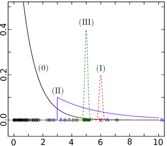
Figure 1: Outlier cases. The null case (0) is standard Exponential $X_{i}\sim$Exp(1) for which a realization of 50 points are plotted as open circles. Three outlier cases are considered on top of the null: (I) a single outlier $Y_{1}\sim$Norm$(\mu,0.1)$ plotted for $\mu=6$ with a dashed red line, and a red x mark indicating the outlier; (II) multiple dispersed outliers $Y_{i}\sim 3+$Exp$(1/\beta),~{}i=1,...,5$ plotted with a solid blue line for $\beta=4$ and blue triangles indicating (a realization of) the outliers; (III) multiple clustered outliers $Y_{i}\sim$Norm$(\mu,0.1),~{}i=1,...,5$ plotted with a green dotted line for $\mu=5$, and green dots indicating the outliers.

In addition to the tests mentioned above we also consider a mixture model,

$$f(x)=\pi\alpha\text{exp}\{-\alpha x\}+(1-\pi)\phi(x;\mu,\sigma)~{},~{}\alpha,\sigma>0~{},$$ (10)

where the Gaussian density $\phi(x;\mu,\sigma)$ provides the outlier regime, and $0\leq\pi\leq 1$ is a weight. This model will allow us to classify points as either outliers or not. The Maximum Likelihood estimation (MLE) of this model (10) is done using an Expectation Maximization (EM) algorithm [41]. A LRT of this model versus the null (a pure Exponential) provides p-values, and $n\hat{\pi}$ estimates the number of outliers without requiring sequential testing.

In Fig. 2, the power curves, at level 0.1, for the above test statistics are plotted for different scenarios. For a single outlier (I), most of the tests are exactly identical (by definition), with the exception of the DK and D tests, which are weaker. For multiple dispersed outliers (II), the SS test performs best, and robust versions are slightly less powerful. The mixture is poorly specified and is thus weakest. For clustered outliers (III), the performance of the tests varies greatly. Indeed, the test statistic with the sum in the numerator (SS, SRS) often identifies the cluster of outliers. However, the well specified mixture model is most powerful, also identifying the “outliers” when they are not really outlying but rather a contamination well within the sample.

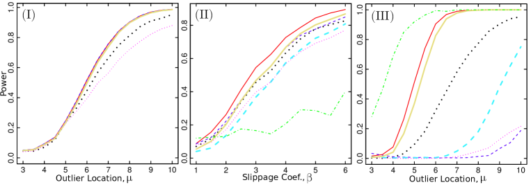
Figure 2: The power curves of multiple tests, at level 0.1, are estimated by repeating the tests on 2000 independent simulations. Three cases are considered: (I) $n=20$, $k=1$, $X_{i}\sim$Exp(1), $i=1,...,19$, $X_{20}\sim$Norm$(\mu,0.1)$, $\mu=3,...,10$; (II) $n=50$, $k=5$, $X_{i}\sim 3+$Exp$(1/\beta),~{}i=46,...,50$, $\beta=1,2,...,6$; (III) $n=50$, $k=5$, $X_{i}\sim$Exp(1), $i=1,2,...,45$, $X_{i}\sim$Norm$(\mu,0.1),~{}i=46,...,50$, $\mu=3,4,...,10$. The mixture model (10) is only estimated in the cases with multiple outliers. The format of the power curves of the statistics are: SS (red solid), SRS with $m=k$ (yellow heavy solid), MS (blue dashed), MRS with $m=k$ (turquoise heavy dashed), D (magenta light dotted), DK (black heavy dotted), and Mixture (green dotted and dashed).

2.5 Outlier test performance with respect to Masking, Swamping, and estimating the number of outliers

We now present simulation studies to expose the degree to which the different test statistics suffer from masking and swamping. This involves three scenarios where tests are afflicted by (I) swamping due to a single outlier, (II) swamping without masking due to dispersed outliers, and (III) swamping with masking due to clustered outliers. This is done by performing the tests on synthetic data for a range of block sizes. The scenarios (I)-(III) correspond to the densities plotted in Fig. 1.

The results are in Fig. 3. Masking is more problematic when large observations are densely clustered (case (III)). Test statistics based on sums overcome masking earlier. Further, the robust tests statistics are less prone to masking – as intended. Swamping is pervasive in block testing, even when there is only a single large outlier. The test statistics based on sums recover from swamping faster than those based on spacings and maxima. As a side note, that the rejection rate decays slowly as the block size surpasses the true block size indicates that the minimal p-value in the sequence of estimates will not reliably indicate the true block size. These problems motivate sequential testing.

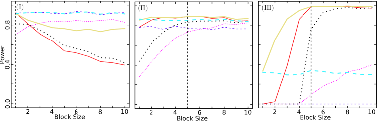
Figure 3: Swamping and masking: From left to right, three cases are illustrated: (I) swamping, (II) swamping without masking and (III) swamping with masking. In all cases, the outlier tests were applied to 2000 independent samples for a range of block sizes ($b=1,2,...,10$). The frequency of these tests being rejected at level 0.1 are plotted. In each case, the true number of outliers is given by the vertical line. The data generating processes for the cases are: (I) $n=30$, $k=1$, $X_{i}\sim$Exp(1), $i=1,...,29$, $X_{30}\sim$Norm$(8,0.1)$; (II) $n=30$, $k=5$, $X_{i}\sim$Exp(1), $i=1,...,25$, $X_{i}\sim 3+$Exp$(1/5),~{}i=26,...,30$; and (III) $n=30$, $k=5$, $X_{i}\sim$Exp(1), $i=1,...,25$, $X_{i}\sim$Norm$(8,0.1),~{}i=26,...,30$. The tests are colour coded: SS (red solid), SRS with $m=k$ (yellow heavy solid), MS (blue dashed), MRS with $m=k$ (turquoise heavy dashed), D (magenta light dotted), DK (black heavy dotted).

2.6 Comparative study of the performance of sequential estimators

We compare inward and outward sequential procedures, again considering the four scenarios visualized in Fig. 1. We use: (i) outward tests with MS, MRS, SS, and SRS test statistics; (ii) the inward procedure with only the MRS test statistic that is necessary to avoid masking and swamping; (iii) the mixture model (10); and (iv) the SRS block test, given the correct number of outliers. This last option, which was the best performing block test in Fig. 2, provides a benchmark.

The dfs for the test statistics were simulated with 50,000 samples from the null model. All tests are done with a level of 0.1. For the outward test, the marginal tests need to have their level $b$ lowered to obtain the overall level of $a=0.1$. For each test, this was done by applying the test on 10,000 independent samples generated from the null, for multiple values of $b$, and selecting $b$ such that $a(b)=0.1\pm 0.005$. The resultant marginal levels are in Table 1. Note how large of an adjusment is needed in the outward test, whereas in the inward test there is no adjustment: $b^{\text{Inward}}=a=0.1$.

n	r	MS	SS	MRS	SRS
50	10	0.018	0.05	0.025	0.049
30	5	0.028	0.055	0.0345	0.0575
15	5	0.025	0.06	0.036	0.056

Table 1: Marginal levels (b) for outward tests for different sample sizes (n), maximal number of outliers (r), and robustness value ($m=r$) to obtain an overall type 1 error level of $a=0.1$

The results, for slightly different specifications of the four cases, and in order of decreasing sample size, are in Tables 2, 3, and 4.

In case (0), where there are no outliers, we see that the inward and mixture procedures have false positive events that estimate a small number of outliers, whereas the outward procedures falsely identify large numbers of outliers. In case (I) of the sequential procedures, the inward test is most powerful at identifying the single outlier, even matching the power of the block test. The outward tests are substantially weakened, even with relatively small $m=5$. The inward test provides superior estimation of outliers, whereas the other tests tend to overestimate. In case (II), with a cluster of outliers, both our benchmark (the block test) and the inward test perform poorly. They are outperformed by the outward test, which has the advantage of first encountering the large gap between the main data and the outliers before the dense outliers. However, here the mixture approach is both the most powerful and accurate in estimating outlier numeracy. In case (III), with multiple dispersed outliers, all of the inward and outward approaches are similarily competitive, while being slightly dominated by the block test. The mixture approach is weak since the outlier component is poorly specified. For the outward procedure, the MS/MRS statistic dominates the SS statistic.

In summary, the inward procedure with the MRS test statistic is more computationally convenient than the outward procedure, commits less severe false positives, and can even be more powerful when identifying single or multiple dispersed outliers. In the event of a dense cluster of outliers, a mixture approach can be more computationally convenient and powerful than the outward approach. Within the outward approach, the MS statistic was superior, and robust modifications performed similarly.

Case	Quantity	MS Out	SS Out	MRS Out	SRS Out	MRS In	Mix	SRS Block
(0)	Rej. Rate	0.11	0.10	0.11	0.10	0.10	0.14	0.10
(0)	$\widehat{k}$	(3,6,9)	(5,9,10)	(3,6,9)	(5,9,10)	(1,1,3)	(2,2,4)
(I)	Rej. Rate	0.30	0.22	0.30	0.22	0.64	0.09	0.69
(I)	$\widehat{k}$	(2,3,6)	(2,5,10)	(2,3,7)	(2,5,10)	(1,1,2)	(2,2,2)	$=1$
(II)	Rej. Rate	0.91	0.75	0.89	0.75	0.04	0.95	0.38
(II)	$\widehat{k}$	(5,7,8)	(5,7,10)	(5,7,9)	(5,7,10)	(1,9,10)	(5,5,6)	$=5$
(III)	Rej. Rate	0.96	0.96	0.97	0.96	0.95	0.63	0.98
(III)	$\widehat{k}$	(5,6,8)	(4,6,10)	(5,6,9)	(4,6,10)	(6,7,10)	(3,10,10)	$=5$

Table 2: $n=50$, $m=10$. Summary of tests over 5000 repeated simulations of four cases: (0) the null case ($X\sim$Exp(1)), (I) a single large outlier ($X_{i}\sim$Exp(1), $i=1,...,49$; $X_{50}\sim$Norm$(7,0.1)$), (II) a cluster of multiple outliers ($X_{i}\sim$Exp(1), $i=1,...,45$; $X_{i}\sim$Norm$(5,0.1),~{}i=46,...,50$); (III) multiple dispersed outliers ($X_{i}\sim$Exp(1), $i=1,...,45$; $X_{i}\sim$ max$(\{X_{i}:i=1,...,45\})$+Exp$(1/5)$, $i=46,...,50$). The rejection rate and the median and quartiles of the estimated number $\widehat{k}$ of outliers (in the event of a rejection) are given in alternating rows.

Case	Quantity	MS Out	SS Out	MRS Out	SRS Out	MRS In	Mix	SRS Block
(0)	Rej. Rate	0.11	0.11	0.11	0.11	0.11	0.16	0.10
(0)	$\widehat{k}$	(2,3,5)	(4,5,5)	(2,4,5)	(3,5,5)	(1,1,3)	(2,2,5)
(I)	Rej. Rate	0.45	0.32	0.43	0.33	0.72	0.08	0.75
(I)	$\widehat{k}$	(1,2,3)	(1,3,5)	(1,2,3)	(1,2,5)	(1,1,2)	(2,2,2)	$=1$
(II)	Rej. Rate	0.72	0.63	0.73	0.64	0.08	0.96	0.36
(II)	$\widehat{k}$	(3,4,5)	(3,4,5)	(3,4,5)	(3,4,5)	(4,5,5)	(3,3,3)	$=3$
(III)	Rej. Rate	0.87	0.86	0.89	0.86	0.88	0.50	0.90
(III)	$\widehat{k}$	(2,4,4)	(2,4,5)	(2,4,5)	(3,4,5)	(3,4,5)	(2,5,7)	$=3$

Table 3: $n=30$, $m=5$. Summary of tests over 5000 repeated simulations of four cases: (0) the null case ($X_{i}\sim$Exp(1)), (I) a single large outlier ($X_{i}\sim$Exp(1), $i=1,...,29$; $X_{30}\sim$Norm$(7,0.1)$), (II) a cluster of multiple outliers ($X_{i}\sim$Exp(1), $i=1,...,27$; $X_{i}\sim$Norm$(5,0.1),~{}i=28,29,30$), (III) multiple dispersed outliers ($X_{i}\sim$Exp(1), $i=1,...,27$; $X_{i}\sim$ max$(\{X_{i}:i=1,...,27\})+$Exp$(1/5),~{}i=28,29,30$). The rejection rate and the median and quartiles of the estimated number of outliers (in the event of a rejection) are given in alternating rows.

Case	Quantity	MS Out	SS Out	MRS Out	SRS Out	MRS In	Mix	SRS Block
(0)	Rej. Rate	0.11	0.11	0.11	0.11	0.08	0.16	0.10
(0)	$\widehat{k}$	(2,3,4)	(3,5,5)	(2,3,5)	(3,5,5)	(1,2,4)	(2,3,5)
(I)	Rej. Rate	0.25	0.22	0.23	0.20	0.30	0.14	0.30
(I)	$\widehat{k}$	(2,3,4)	(2,4,5)	(2,3,4)	(2,4,5)	(1,2,3)	(2,2,4)	$=1$
(II)	Rej. Rate	0.42	0.42	0.43	0.41	0.04	0.93	0.13
(II)	$\widehat{k}$	(3,4,5)	(4,5,5)	(3,4,5)	(3,5,5)	(3,4,5)	(3,3,3)	$=3$
(III)	Rej. Rate	0.63	0.62	0.64	0.62	0.63	0.37	0.66
(III)	$\widehat{k}$	(2,3,4)	(2,4,5)	(2,3,4)	(2,4,5)	(2,3,5)	(2,3,4)	$=3$

Table 4: $n=15$, $m=5$. Summary of tests over 5000 repeated simulations of four cases: (0) the null case ($X_{i}\sim$Exp(1)), (I) a single large outlier ($X_{i}\sim$Exp(1), $i=1,...,14$; $X_{15}\sim$Norm$(4,0.1)$), (II) a cluster of multiple outliers ($X_{i}\sim$Exp(1), $i=1,...,12$; $X_{i}\sim$Norm$(4,0.1),~{}i=13,14,15$), (III) multiple dispersed outliers ($X_{i}\sim$Exp(1), $i=1,...,12$, $X_{i}\sim$max$(\{X_{i}:i=1,...,12\})+$Exp$(1/5),~{}i=13,14,15$). The rejection rate and the median and quartiles of the estimated number of outliers (in the event of a rejection) are given in alternating rows.

2.7 Robustness to null mis-specification

In practice, the correct specification of the null/main model is of considerable importance. Here, the sensitivity of the rate of false positives (level), and true positives (power), to the degree of misspecification of the null are exposed via a simulation study, for the battery of test statistics implemented in block tests. We consider simulating data from a Weibull df,

$$F(x)=1-\text{exp}\{-(x/\tau)^{\kappa}\},~{}x\geq 0,~{}\tau,\kappa>0~{},$$ (11)

which is Exponential ($\alpha=\tau^{-1}$) when $\kappa=1$, is fat tailed for $\kappa<1$, and becomes concentrated at $\tau$ as $\kappa$ becomes large. The results of the simulation study are presented in Fig. 4 and can be described as follows.

Case (a) concerns the rate of false positives (type 1 error) where we test for $r=3$ outliers, with level $a=0.1$, in a Weibull (11) sample of size $n=30$, for a range of shape parameters $\kappa$, without outliers. When $\kappa<1$ the df is fat tailed, having many events that are large, and thus the tests falsely identify many points as outliers. This is problematic in practice (with small to moderate sample sizes), because one does not know what the true null model is. For instance, with $n=30$, even when we consider the true df as an alternative model versus the Exponential, and using the powerful LRT, 50 percent of the time (for $\kappa\approx 0.6$) we will not reject the Exponential model at a level of 0.1. In this case, when falsely retaining the Exponential model, the type 1 error will be between 0.3 and 0.5, depending on the selected test statistic. The Kolmogorov-Smirnov (KS) test of compatibility of the data with the Exponential df is even less powerful, allowing for more severe false positives.

Case (b) considers the frequency of true positives (power). The setup is the same as above, but 3 dispersed outliers are included. When the Weibull df becomes less fat tailed, the power of the sum tests (SS, SRS, MS, and MRS) decreases whereas the power of the D and DK tests increases. Here, with $n=30$, for the tests of the Weibull versus the Exponential, including the outliers in the sample, there is a high probability (0.6-0.8) of not rejecting the Exponential model when $1<\kappa<1.5$, where the power of some of the tests is weakened.

It is clear that the power, and especially the level, are highly sensitive to the validity of the Exponential model, and misspecification of the null can lead to erroneous inference. This has important implications for the next section where the test is used when the tail of the null df is only approximately Exponential or Pareto.

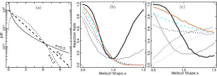
Figure 4: Test robustness Panel (a): The Weibull pdf (11) plotted for parameters $(\kappa,\beta)$ equal to $(0.5,0.4),~{}(1,1)$ and $(1.5,1.5)$. Panel (b): The frequency of rejection of the null of no outliers, at level 0.1, in the presense of no outliers, for block tests for $r=3$ outliers, assuming an Exponential null model, when the data is generated from a Weibull for a range of shape parameters $\kappa$. Panel (c): The frequency of rejection of the null using a level 0.1, of the block tests for $r=3$ outliers, with the same setup as frame (b), except that 3 outliers are truly present. The models for the cases are: (b) $X_{i}\sim$Weibull$(\kappa,1)$, $i=1,...,30$; (c) $X_{i}\sim$Weibull$(\kappa,1)$, $i=1,...,27$, $X_{i}\sim$max$(\{X_{i}:i=1,...,27\})+$Exp$(1/3),~{}i=28,29,30$). For each case, simulation and testing were performed 1000 times for $\kappa$ sweeping 0.5 to 1.5. The tests are colour coded: SS (red solid), SRS with $m=r$ (yellow solid), MS (blue dashed), MRS with $m=r$ (turquoise heavy dashed), D (magenta light dotted), DK (black dotted). In both frames, the black heavy solid line is the power of the LRT of the Weibull versus the Exponential on the data (including outliers). Similarily the grey heavy solid line is for the Kolmogorov-Smirnov test.

3 Case studies of “Dragon Kings”

3.1 Outliers and dragon kings

Outlier detection relative to an Exponential df, $E\overset{\text{iid}}{\sim}\text{Exp}(\alpha)$, has been primarily motivated by reliability engineering applications. Switching perspective from reliability to risk, the transformed variable $X=u\exp\{E\}\overset{\text{iid}}{\sim}\text{Pareto}(\alpha,u)$, has the heavy-tailed Pareto df,

$$F(x)=1-(x/u)^{-\alpha},~{}x\geq u,~{}\alpha>0~{},$$ (12)

that is typically used for modeling extremes in both natural and social sciences: earthquake energies, the df of runs of stock prices, claims in non-life insurance, etc. [13, 37, 38, 48]. Simply put, the logarithm of a Pareto tail is an Exponential tail, and thus these models are connected.

The Pareto df is unique in that it is scale invariant [10, 29], suggesting that events of all sizes – including extremely large ones – are generated by a single mechanism operating at different scales. This feature allows this single (simple) df to represent a broad range of event sizes. Thus, if a phenomenon is scale invariant, then extreme events are not predictable as there is nothing to distinguish these events from their smaller siblings, other than their resultant size. This reasoning has been advanced to explain the extreme difficulties in forecasting large earthquakes [19]: according to the approximate scale invariance of the Gutenberg-Richter law, large earthquakes are just earthquakes that started small… and did not stop growing.

However, a number of studies have found either strong or, in other cases, suggestive evidence that there are extreme events “beyond” the Pareto sample [49, 53], i.e., outliers. From this observation, the concept of the “Dragon King” (DK) was born [49]. DK embody a double metaphor implying that an event is both extremely large (a king [28]), and born of unique origins (dragon) relative to its peers. The hypothesis advanced in [49, 53] is that DK events are generated by a distinct mechanism (e.g., positive feedback) that intermittently amplifies extreme events, leading to the generation of runaway disasters as well as extraordinary opportunities/successes. That is, it questions the assumption that the mechanisms of nucleation and growth remain identical over the spectrum of relevant scales of size, space, and time. Due to the uniqueness of such events, there is hope that such extremes may exhibit precursory signs, disclosing some predictability.

Examples of such DK events have been proposed to include failures of material systems, landslides and some large earthquakes in geophysics, financial crashes in economics, and epileptic seizures and human parturition in biology. A neat example is the DK status of the agglomeration of Paris (resp. London) departing from the Zipf’s law of French (resp. British) agglomerations [28, 39]. While being technically an outlier, Paris (London) is absolutely key to understanding the geo-political-economic evolution of France (UK) over previous centuries and decades. It is not an inconvenient “outlier” that should be thrown away in order to retrieve a clean Zipf law [44]. In other words, the DK Paris (London) arguably plays a dominant role in the whole dynamics of France (UK), even if it uniquely departs from the statistics applying to all the other agglomerations. Another instance of this is in risk management where the empirical tail of losses departs significantly from the loss distribution. One may be tempted, or even feel more principled, in retaining a simple model which fails to account for the largest extremes. For instance, one may wish to use models from EVT, however in the presence of DK – namely where there is a contaminating mass in the extreme tail – the theorems of EVT do not apply, and a different approach to modeling the extremes must be taken. Especially in cases where the largest events dominate the total losses, identifying and attempting to properly model an outlying tail – at least to be considered as a scenario within an ensemble – is of primary importance.

Identifying DKs with convincing statistical significance is a prerequisite to the investigation of their origin, understanding their generating mechanisms, and developing forecasting methods, controls, and resilient system designs. Motivated by these considerations, five case studies are considered below where we test for and try to detect DK events as statistical outliers.

3.2 Financial crashes

It is well known that crashes in the financial markets occur frequently and can have a significant effect not only on market participants, but also on the broader economy. Thus, being able to predict large risks in the market is an ability desired not only for private financial gain, but also to develop responsible policies by central banks and treasuries. The IMF and the ECB, among others, are actively engaged in developing advance warning systems targeting future systemic banking and economic crises. The financial markets have been thought to be scale invariant / fractal  [36, 50] and thus both extreme and unpredictable. But, are the most extreme crash events outliers? If they are, are they dragon kings (in the sense of presenting a degree of predictability)? Here, we address only the first question.

In [16], it was found that the degree of self-excitation / positive feedback of price fluctuations increases in the neighbourhood of a financial crash, providing hope of predictability. In [24, 25], the samples of crashes and runs of negative price changes (drawdowns) were found to contain outliers. More recently in [17], it was found that there are outliers in the sample of crashes – being measured as $\epsilon$-drawdowns (defined below) – and that the sample is well described by a Pareto df. In [17], a modification of the DK test (9) was proposed and employed. However this test contains an error in the df of the marginal test statistics. We thus revisit this problem.

Anticipating multiple dispersed outliers, we apply the MRS test statistic (7) inwards. In such a case, the inward procedure should have similar power to the outward procedure (Sec. 2.6), while being easier to implement. This ease of implementation makes it convenient to apply the test for a variety of sample sizes, providing more robust results.

3.2.1 Definition of drawdowns and drawups

A peak-to-valley measure of the size of intra-day financial crashes is considered: an $\epsilon$-drawdown (hereforth referred to simply as a drawdown) is the total cumulative return of a negative run in price over time, with some specified tolerance for small positive changes along the way [26]. A drawup is its´ positive counterpart. This is an interesting measure of risk because it captures the transient dependence of price changes in time, whereas studying the unconditional df of returns does not.

More specifically, considering one trading day $\left[t_{0},t_{1}\right]$, prices taken at intervals of width $\Delta$ are $p_{i}=p(t_{0}+i\Delta)$, $i=1,...,n=\lfloor(t_{1}-t_{0})/\Delta\rfloor$. The returns are then $r_{i}=\text{log}(p_{i}/p_{i-1})$. One starts at the first negative return $i_{0}=\text{min}\{i:r_{i}<0\}$. Then, the cumulative return,

$$r_{i_{0},i}=\sum_{j=i_{0}}^{i}r_{j}=\text{log}(p_{i}/p_{i_{0}}),~{}i>i_{0}~{},$$ (13)

tracks the negative growth of the drawdown, continuing for $i=i_{0},i_{0}+1\dots$ until the first value of $i$, say $i_{2}$, such that the cumulative return has appeared to reverse direction, relative to its lowest point:

$$r_{i_{0},i_{2}}-\text{min}_{i_{0}\leq j\leq i_{2}}r_{i_{0},j}>\epsilon\sigma~{}.$$ (14)

In eq. (14), $\epsilon\geq 0$ is a tuning parameter for the tolerance of moves in the opposite direction, and $\sigma$ is the standard deviation of the returns from the previous trading day. The inclusion of $\sigma$ makes the tolerance adaptive, which allows for volatity regimes.

Finally, stepping backwards from $i_{2}$, which is the index of a positive change, the drawdown is defined to have occured from the start $i_{0}$ to the lowest point, which occurs at $i_{1}=\text{argmin}_{j\in(i_{0}\leq j\leq i_{2})}r_{i_{0},j}$. From the next index, $i_{1}+1$, a drawup is defined to begin and computed in a similar way. Drawdowns and drawups alternate in this contiguous way, for the entire trading day.

3.2.2 Outlier detection

The data considered are the tick data for the most actively traded Futures Contracts on the American and European Indices, from January 1, 2005 to December 30, 2011. The drawdowns were computed for each contract with $\Delta=30$ seconds and $\epsilon=1$. The adaptive tolerance in (14) was given by $\sigma$ being the standard deviation of the returns from the previous trading day. The $\sigma$ of the previous day was also used to normalize the drawdowns to make drawdowns comparable across different market regimes.

Outlier detection of the normalized drawdowns is summarized in Fig. 5 and described below. In panel (a), for contracts thought to contain an outlier, the largest 5000 drawdowns are plotted according to their empirical CCDF. Further, the Pareto CCDF with MLE parameter for the 500 largest points is plotted. The estimated parameters $\alpha$ were between 4.1 and 4.8. For all indices, the fit is qualitatively good for the bulk of the data, with the exception of apparent outliers, and some differences in the tail. For instance, the tail of the CCDF for DAX (green) curves down. In addition, for several of the contracts, the empirical CCDF drops beneath the Pareto fit before crossing back to form the outlying empirical tail. This could suggest an amplification mechanism operating above a threshold size.

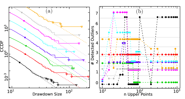
Figure 5: Financial Market Crashes. (a): The 5000 largest drawdowns for each of the 8 futures contracts thought to contain outliers, plotted according to their empirical CCDF in double logarithmic scale. For clarity, each CCDF above the black one is multiplied by 10 relative to the one beneath it. The Pareto with MLE parameter for the top 500 points is given by the dashed lines, starting at the solid dot. The triangles identify the points that were identified as outliers based on the interpretation of panel (b). The CCDF are colour coded: black is ES, red is CAC, green is DAX, blue is FTSE, turquoise is SMI, magenta is IBEX, grey is NQ, and DJ is orange. AEX, OMX, and STOXX were not found to have outliers and were thus omitted from the figure.
(b): The number of identified outliers is plotted against sample size where the MRS test (7) with level $a=0.1$ has been applied inward with $m=r=10$, for a range of sample sizes $n$, for each contract in (a) with the same colour coding. (see online version for colour)

For each data set, the inward test – with MRS test statistic, $m=10$, level $a=0.1$, and a range of sample sizes $n=10,\dots,1000$ – was performed. For all contracts, excluding AEX, OMX, and STOXX, at least 1 outlier was found and are indicated in Panel (b) of Fig. 5. For some of the contracts, the results are quite stable across sample size (e.g., CAC (red) and FTSE (blue)). For others, the impurity of the df plays a role in the interpretation. For instance, for DAX (green), two outliers are detected once the test is restricted to the bent-down tail. For ES (black), choosing between zero and seven outliers is more subjective – are there multiple outliers, or does the tail grow heavier? For IBEX, it is clear that the identification of seven outliers is due to the dip in the empirical CCDF occuring between drawdown size of twenty and thirty. The alternative choice of 1 outlier is more stable with respect to a broad range of values of $n$. The interpreted outliers are indicated in panel (a).

The largest outliers coincide with major news events: The 07 July 2005 London bombings coincided with the largest outliers of CAC, DAX, FTSE, SMI, and IBEX – all being based on European indices. Further, DAX and CAC each have an outlier corresponding to the “Mini Flash Crash” of 27 Dec. 2010 (e.g., see [6]). All American contracts (ES, DJ, and NQ) have their largest outliers coinciding with the infamous “2010 Flash Crash” of 6 May 2010. We thus observe that outliers occur either due to some exogenous impacts (London bombings) or as a result of an endogenous transiently unstable dynamics (flash crash). Indeed, in [16, 15], it was suggested that financial markets exhibit a significant endogeneity or “reflexivity”, in the sense that nowadays up to 70-80% of trades occurring at the time scales of fractions of seconds to tens of minutes are motivated (or triggered) by previous trades. In this framework [16, 15], dragon kings emerge when the market dynamics become critical and super-critical, that is when the future trades are triggered essentially only by previous trades and not by news, making the financial markets essentially self-referential in these periods. Thus, we can conclude that some of the outliers that we have diagnosed can be classified as dragon king drawdowns.

3.3 Nuclear accidents

We consider events (incidents and accidents) occurring at nuclear power plants, studied in [56]. We consider both the property damage (in US Dollars), and a logarithmic measure of the amount of radiation released called the Nuclear Accident Magnitude Scale (NAMS) [47]. Since the disaster at Fukushima in 2011, Nuclear power has come under major public scrutiny. Further, the level of risk that the nuclear industry claims is consistently much lower than statistical analysis of past events indicates [52]. Thus, it is crucial to arrive at a better understanding of the true risk level in this critical application.

The disaster occurring at Fukushima in 2011 is expected to cost 170 Billion USD. Fukushima, being the most costly event thus far, accounts for 60 percent of the total damage to date (including itself) caused by the 184 events in the dataset. Within a pure Pareto description, this value of 60 percent corresponds to a tail exponent $\alpha=0.4$ (see [14] p.169 and eq.(4.48) in [48]), clearly qualifying nuclear accidents as extreme risks. It is instructive to ask whether a very heavy Pareto tail is sufficient to account for these extreme risks or, alternatively, if the tests discussed here could identify outliers / DKs in this data.

The logarithmic radiation measure, NAMS, as well as the logarithm of damage (in millions of USD) are plotted in Fig. 6 according to their empirical CCDFs. For NAMS, there is a cluster of four points that appear to be outlying relative to the Exponential df with MLE parameter $\hat{\alpha}_{NAMS}=0.72~{}(0.3)$, which is qualified by a straight line in the logarithmic plot. For logarithmic damage, there are three spaced out events that appear to be outlying relative to the Exponential df with MLE parameter $\hat{\alpha}_{\$}=0.61~{}(0.14)$.

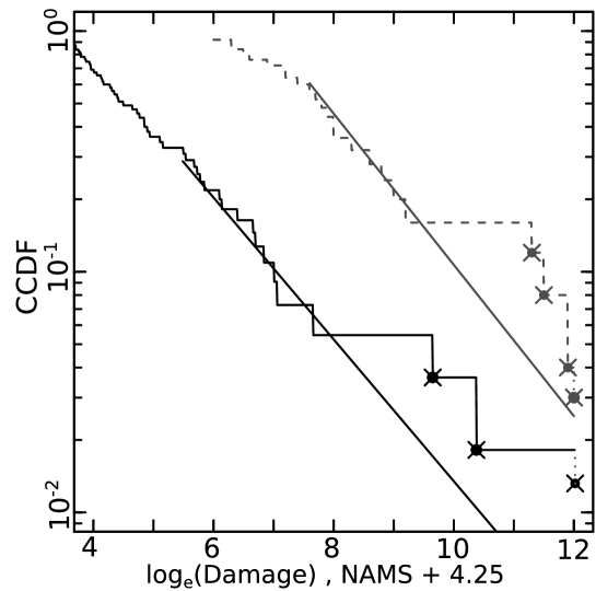
Figure 6: Nuclear Power Plant Accidents: the CCDF of the log of damage in millions of US Dollars due to accidents (black solid), and the CCDF of the log radiation release (NAMS, in grey dashed) shifted by 4.25 units for visibility. The fitted lines are MLE for the Exponential df above 3.5 with the observations with x marks censored. The estimates are $\widehat{\alpha_{\$}}=0.61~{}(0.14)$, $\widehat{\alpha}_{NAMS}=0.72~{}(0.3)$.

Not surprisingly the df of NAMS and damage are similar, and there is a positive relationship between them: Considering 17 events with substantial radiation release (NAMS$>0$) occurring at Sellafield, UK, a linear regression of the logarithm of damage versus NAMS yields an intercept of $2.013~{}(0.9),~{}p=0.043$ and a slope of $1.3~{}(0.34),~{}p=0.0015$ with coefficient of determination $R^{2}=0.5$. This relationship should be specific, depending on the property development near the plant. Focusing on the (expected) outliers in both datasets: Fukushima, Chernobyl, and TMI have both damage and NAMS values available. Of these three common values, all are outliers in NAMS, and all but TMI are outliers in damage, presumably due to a lack of property development in the vicinity of TMI. In fact, Fukushima has caused sixty times more damage than TMI despite having a lower radiation release. Thus, it appears that there is a DK mechanism by which radiation release events above a threshold become runaway disasters, which, depending on the location, may translate into damage disasters.

We now test the outliers with a number of the aforementioned tests. The results are presented in Tab. 5 and summarized below. First considering NAMS, since the outliers are clustered, we know (Sections 2.4 and 2.6) that the mixture approach will be most powerful, with an outward test being less powerful, and both tests based on maxima and inward approaches being weakest. Indeed this is reflected by the results in the table. Further, in Fig. 6, the Exponential CCDF is fit to the empirical data for the top $n=15$ points. For the top $n=20$, the empirical CCDF is concave, and thus the power of the tests is weakened (Sec. 2.7).

Since the mixture approach is the most sensible specification here, and the weaknesses of the other tests are well understood, we employ the mixture approach for interpretation, with $n=15$. The model (10) is estimated by an Expectation Maximization algorithm [41]. The estimates of this (alternative) model are $(\widehat{\pi}=0.74,\widehat{\alpha}=0.80,\widehat{\mu}=7.68,\widehat{\sigma}=0.29)$. Under this model, the probability that the largest through the fourth largest points come from the DK regime are $(0.97,0.97,0.97,0.94)$, whereas the fifth largest and smaller points have virtually zero probability, indicating 4 DK points. Considering a pure Exponential null model with the MLE $\widehat{\alpha_{0}}=0.6$, the LRT of the null versus the alternative provides a p-value of 0.01, indicating signficance of the DK points.

Next, the damage value outliers are tested. Unlike in the NAMS case, the three outliers here are relatively dispersed. Once the test considers a sample above $n=20$ where the empirical CCDF has a kink (Fig. 6), the null of no outlier is consecutively rejected by a number of tests (for $n=19,18,\dots,8$).

With the evidence of outliers in both NAMS and damage, and their positive relationship, it seems warranted to conclude that the largest nuclear accidents are indeed dragon kings.

Data	$n$	$r=m$	MRS	SRS	MS Out	MRS In	Mix	DK
NAMS	$20$	$4$	$0.84$	$0.90$	$0,~{}0.67>0.03$	$0,~{}0.84$	$\mathbf{0.06}$	$0.33$
NAMS	$15$	$4$	$0.48$	$0.17$	$\mathbf{4,~{}0.015<0.03}$	$0,~{}0.48$	$\mathbf{0.01}$	$0.13$
Damage	$20$	$3$	$0.23$	$0.15$	$0,~{}0.07>0.04$	$0,~{}0.23$	$1$	$\mathbf{0.09}$
Damage	$18$	$3$	$0.11$	$\mathbf{0.035}$	$\mathbf{3,~{}0.02<0.04}$	$0,~{}0.11$	$0.96$	$\mathbf{0.05}$
Damage	$10$	$3$	$\mathbf{0.07}$	$\mathbf{0.04}$	$\mathbf{3,~{}0.01<0.04}$	$\mathbf{3,~{}0.08}$	$0.18$	$\mathbf{0.05}$

Table 5: p-values for outlier tests of both NAMS and damage data, for the upper $n$ points, for $r$ outliers (with robustness value $m=r$). Bold values indicated significance at a level of $a=0.1$. Block tests performed include: MRS (7), SRS (5), mixture likelihood ratio (10), and the DK test (9). Further, the MS (6) test was applied outward (MS Out), with the number of identified outliers, the p-value, and the adjusted level (to achieve $a=0.1$) given. We find $0.02$ for the nominal p-value and $0.04$ for the adjusted level to control type 1 error at a level of 0.1. Finally, the MRS (7) test was applied inward (MRS In), with the number of identified outliers, and the p-value of the test for the largest point given.

3.4 Stock returns

An issue of debate is if the 1987 stock market crash (Black Monday) was an outlier. We focus on [45], which is the most recent study on this problem. In [45], considering daily returns on the Dow Jones Industrial Index, from 3 January 1977 to 31 January 2005, it was claimed that Black Monday is not an outlier. In further detail, the returns were whitened by taking the residuals of a standard AR(1)-GARCH(1,1) model estimated on the returns. Next, the two largest whitened returns $X_{(2)}$ and $X_{(1)}$ were tested as outlying. The test used relies on the GPD approximation (2) of the tail of the sample, and requires an estimate of the tail parameter $\alpha$. A sample size of $n=732$ was used to estimate $\alpha$. The test statistic $T_{r}=X_{(r)}/X_{(r+1)}$, comparing $X_{(r)}$ to the previous (next largest) order statistic $X_{(r+1)}$, was used to test if $X_{(2)}$ and $X_{(1)}$ were outlying. Testing outward, with a level of 0.05, neither of these points were identified as outliers.

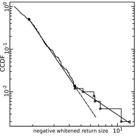
Figure 7: Stock Returns: The rough line provides the empirical CCDF of the magnitude of the 500 largest whitened returns of the Dow Jones Industrial Index from 3 January 1977 to 31 January 2005. The solid lines between solid dots provide Pareto model estimates for two magnitude layers. The dashed line extends the slope of the first layer for comparison with that of the second.

To evaluate the approach taken in [45], we first plot the CCDF of the 500 largest negative whitened returns in Fig. 7. This plot was not provided in [45], but is clearly essential to assessing above which threshold the GPD approximation (2) is sound. A few important points are apparent from the figure: Firstly, the CCDF above the $200$ largest observations is shallow/concave, and thus considering more than 200 points (i.e., 732 in [45]) in the sample will weaken the test (i.e., the estimate of $\alpha$ will be too small). Secondly, the second largest point is similar in magnitude to the largest. Thus, the test using $T_{1}=x_{(1)}/x_{(2)}$ will be masked by $x_{(2)}$, and not rejected. Finally, the top 6 or 7 points seem to follow a heavier tailed df. Thus, 6 or 7 points should be tested as outlying, rather than only 2, and a sum test statistic, measuring the cumulative departure of the empirical tail, could be more powerful.

First, we consider estimating a Pareto df with two layers. The first layer, containing 193 points, covers $1.97<x\leq 4.45$ and has MLE $\hat{\alpha}_{1}=3.8$. The second layer, containing the 7 largest points, covers $4.45<X$ and has MLE $\hat{\alpha}_{2}=1.8$. Given that the first layer model is true, there is a $p=0.02$ probability of observing such an extreme difference between the estimated parameters. This two layer model appears to describe the empirical CCDF well (Fig. 7). Next, a single layer model for the top 200 points, covering $4.45<X$ was estimated with MLE $\hat{\alpha}_{0}=3.9$. The likelihood ratio test of the two layer versus one layer model rejected in favour of the two layer with p-value $0.07$. Further, applying the SS test for $r=6$ with the top $200$ points rejects that there are no outliers with $p=0.04$. Finally, applying the DK test for 6 outliers, for upper sample sizes ranging from 20 to 200, all tests had $p<0.04$. Thus it appears that the 6 largest points are outlying.

The largest one is, unsurprisingly, “black monday” Oct. 19, 1987, which is unambiguously classified as an outlier. An enormous literature has dwelled on its possible origin with a lot of confusion as no simple proximate cause can explain its occurrence. We find more compelling the story that it marked the end of a large financial bubble and thus corresponded to its burst [51, 50, 26]. The second largest event occurred on “black friday” Oct. 13, 1989 and is usually associated with a fall of the junk bond market (https://en.wikipedia.org/wiki/Friday_the_13th_mini-crash). The third largest loss corresponds to the first day of reopening of the US stock markets on Sept. 17, 2001 after Sept. 11, 2001. It is not clear to us how to interpret the fourth largest loss that happened on Nov. 15, 1991. The fifth largest loss on Oct. 27, 1997 is analyzed in details in [50], which paints a picture much richer than the usual story that this was a global stock market crash caused by an economic crisis in Asia. This loss can actually be seen also as a partial burst of a bubble that had been surging in the few previous years (recall the famous quip on the “irrational exuberance” of the stock markets by Alan Greenspan, then the Chairman of the US Federal Reserve, on Dec. 5, 1996 (http://www.federalreserve.gov/boarddocs/speeches/1996/19961205.htm)). The sixth largest loss on Nov. 9, 1986 is not clearly associated with any exogenous cause, to the best of our knowledge. These six outliers are part of the list found by other researchers (e.g. [18]).

3.5 Fatalities in Epidemics

We now study the number of fatalities caused by outbreaks of bacterial, viral, and parasitic diseases (epidemics). A dataset for this, with 1,368 events covering the period from 1900 to 2015, was provided by [21]. The dataset excludes, and in some case provides only national fatalities for, pandemic events (spanning multiple countries). Thus the dataset was complemented with the well known Spanish (1918), Asian (1957), and Hong Kong (1968) Influenza pandemics, which each caused in excess of 1 million fatalities [40]. Further, the 2009 H1N1 “Swine” influenza pandemic, which was estimated to cause upwards of 150,000 fatalities [46], was also included. All epidemics and pandemics will be simply referred to as events.

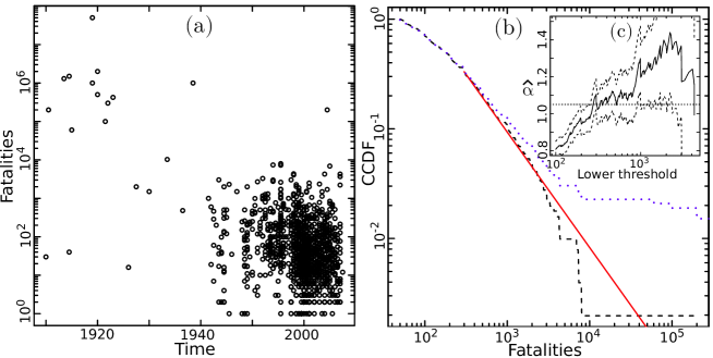
Figure 8: Epidemic Fatalities: (a) scatterplot of 1,368 epidemic fatalities from 1900 to 2015. (b) The CCDF of the 507 events in excess of 50 fatalities from 1960-2015 (black dashed), its Pareto tail fit with lower threshold $u=300$, and MLE $\hat{\alpha}=1.05~{}(0.08)$, and the CCDF of the 523 events in excess of 50 fatalities from 1900-2015 (blue dotted), having 9 events beyond the window. The inner panel (c) plots the Pareto tail estimate for samples exceeding lower thresholds ranging from 50 ($n=507$) to 4,300 ($n=20$) for the time period from 1960-2015 (i.e., the black dashed CCDF). The level 1.05 is given by the horizontal line.

From Panel (a) of Fig. 8, it is clear that over time the dataset has become more complete, in particular for small event sizes. Further, in the period from 1900-1960, 13 events have more than 10,000 fatalities (0.21 per year), whereas in the period from 1960-2015, only 1 such event does (0.02 per year). Notwithstanding potential changes in the true frequency of events, this is obviously a highly significant difference. These historical extreme events – Influenzas, Bubonic plagues, Cholera, etc. – have largely been eradicated through sanitation, vaccines and antibiotics.

Considering the period from 1900 onwards, many changes have occurred that should have influenced both the incidence and severity of events. Due to data incompleteness, the rate of events cannot be studied.

Despite this, the sample in excess of 50 fatalities from 1960 onwards, containing 507 points, is roughly stationary in severity. For instance, when repeatedly (1000 times) sampling 100 points from the 507 points, splitting the 100 points into two equal subsamples, and testing their distributions for equivalence with the KS test, only 12.6 percent of p-values were less than 0.1. Thus, the modern sample – spanning the 55 years following 1960 – may be used as a proxy to evaluate the outlyingness of the historical extremes, or at least to evaluate how outlying they would be if they were to occur now.

The events in excess of 50 fatalities from both 1900 onwards and 1960 onwards are plotted according to their CCDF in Panel (b) of Fig. 8. The sample from 1960 approximately has a Pareto tail (see Panel (c)) with parameter around 1.05 (0.08) for the 168 points above the lower threshold of 300. With increasing lower truncations, the estimated parameter increases (as the CCDF bends down), however this is not a significant departure from the estimated tail. For instance, the Anderson-Darling test for the fit of the top 168 points gives a p-value of 0.8. The tail of the sample from 1900 onwards is skewed both by the inclusion of historic large events, and also by the absence of their smaller siblings, which were not recorded.

The value of the exponent $\alpha\approx 1$ is reminiscent of Zipf’s law, which is known to derive quite robustly from the interplay between three simple ingredients [44]: birth, proportional growth (also known as “preferential attachment” in network theory) and death. If the variance of the proportional growth component is large, the df of event sizes converges to a power law with exponent $\alpha\approx 1$. These ingredients are arguably minimum constituents of epidemic processes and rationalize our finding $\alpha=1.05~{}(0.08)$. What is really surprising is the detection of outliers that we present below, which, in some cases, suggests the activation strong amplification processes beyond the proportional growth mechanisms.

We turn our attention to the detection of outliers relative to the approximately stationary data from 1960 onwards. The 14 events in excess of 10,000 fatalities – 13 of which happened before 1960 – are considered. The smallest of these 14 is a Cholera outbreak causing 10,276 fatalities (Egypt, 1947). We start with the weakest possible test, considering as a sample: the 167 points with between 300 and 10,000 fatalities occuring since 1960, plus the aforementioned Cholera outbreak. Testing for a single outlier with the DK test (9) gives a p-value of 0.002. Thus any of the other suspected outliers – including the 2011 Swine Flu event – would be identified as significant outliers also. And, including multiple of these outliers in the sample, and testing them together, would provide even higher significance.

With respect to the mechanism(s) at the origin of these outliers, it is likely that each case may be associated with specific catalysing processes. For one of the largest dragon-kings, the so-called Spanish flu of 1918 which killed an estimated 50 millions people in the world, there is a clear identified amplification mechanism. In this epidemic, about 500–600 million people, a third of the world s population at that time, were infected. The pandemic took five times more lives than the First World War. The first cases of the unknown disease were registered in Kansas, America, in January 1918. By March 1918, more than 100 soldiers fell ill at the US army camp in Funston, Haskell County, where more than 5000 recruits were training for further military operations on the European battlefronts of the First World War. Most of the recruits were farmers, had regular contact with domestic animals and were less resistant to viruses than recruits from cities. The high concentration of personnel in the camp simplified human-to-human transmission. At that time, viruses were not known to medicine, and some doctors had not even accepted the idea that microorganisms could cause disease. Later, the personnel of Funston camp were transferred to Europe by ship, and during the long transatlantic crossing, the virus spread among soldiers coming from other parts of the USA. Upon arriving in Europe, American soldiers infected British and French forces, which in their turn infected German forces in hand-to-hand combat. When Woodrow Wilson, President of the United States from 1913 to 1921, began to receive reports about a severe epidemic among American forces, he made no public acknowledgement of the disease [5]. Moreover, other governments involved in the war made similar decisions – censorship, lies, and even active propaganda – to keep up morale, allowing the disease to continue to spread without any preventive measures. The pandemic was named “Spanish flu” because Spain was a neutral country during the First World War and did not suppress the media, so it was only Spanish newspapers that published honest articles about the severity of the disease – despite the fact that it had originated in the USA and spread initially among American soldiers in the absence of a proper response by the US government. This lack of response was probably due to the US strategic goal of developing a strong political influence in the post-WWI peace process that was to shape international politics in the following decades. In summary, the amplification mechanisms that led to the Spanish flu dragon-king are (i) extremely efficient connectivity between people mediated by movements of soldiers and (ii) rare absence of any prophylactic or treatment measures due to the priority given to the war efforts.

We thus conclude that we found evidence of dragon-kings in the database of epidemic events, including the more recent period post-1960, albeit with a much reduced frequency. For instance, one of our detected outliers, the Swine Influenza pandemic, occurred in 2009. Concerning the AIDS pandemic, which is not included in the dataset, in 2014, 1.2 million [1 million–1.5 million] people died from AIDS-related illnesses, a significant improvement from the maximum reached in 2015 of 2.3 million [2.1 million–2.6 million] deaths from AIDS-related illnesses, with an estimated $\sim 36$ million total deaths since its identification [55, 54]. The evidence we have presented for a dragon-king regime in the dynamics of epidemics suggests that a return of pandemic plagues cannot be ruled out, perhaps catalysed by the severe progressive threats of antimicrobial resistance [8], and climate change.

3.6 City sizes

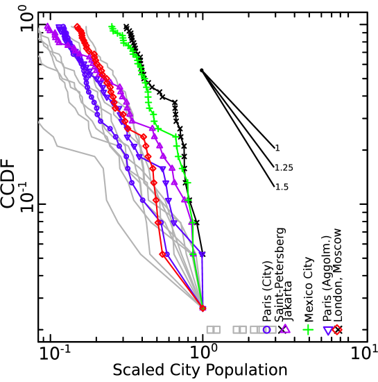
Figure 9: City sizes: plot of the CCDF for the 35 largest cities (and also agglomerations for France) in each of the 14 countries: Brasil, China, France, India, Indonesia, Japan, Korea, Mexico, Nigeria, Pakistan, Phillipines, Russia, the UK, and the USA. The sizes were scaled such that the second largest point (third largest for Russia) in each country has size 1. The scaled largest point (two largest for Russia) are plotted in the bottom right. Each country that is suspected of having outliers is in colour: France (blue circles for cities, blue downward triangles for agglomerations), Russia (black x marks), Indonesia (purple triangles), Mexico (green crosses), and England (red squares).

Within the disciplines of economics, geography and geopolitics (among others), the distribution of city and of agglomeration sizes is of particular interest, due to the importance of urban primacy, and because it constitutes one of the key stylized facts. There is a large literature documenting that the distributions of city and agglomeration sizes follows a Pareto df with parameter close to one (Zipf’s Law) (see e.g. [44] and references therein). There has been some debate over if the df would be better represented by a Lognormal [11, 12, 30], however the debate has been clearly settled in favour of the Pareto for the 1000 largest cities [35]. Note that both the Pareto and Lognormal df’s are generally taken to result from Gibrat’s principle of proportional growth [20] (see [44] for a general derivation).

In [39], the DK test (9) was used to identify outlying population agglomerations for a number of countries, assuming a Pareto tail. Here we consider city sizes rather than agglomerations since this data is available for more countries. We only consider agglomeration sizes for the case of Paris, France for comparison with [39]. Data for 14 large countries were taken from [1]. All tests use the SRS block test statistic for testing the largest point as an outlier, with the exception or Russia where two outliers are tested.

In Fig. 9, the 35 largest cities of each country are plotted according to their empirical CCDF, rescaled in a way to make the largest cities comparable. Since not all of the samples appear to follow a pure Pareto df, results on robustness and testing the tail (Sections. 2.7 and 2.1) are relevant here. First considering French cities, for upper sample sizes of $5<n\leq 35$, the p-value fluctuates in a range of $0.1-0.2$. Thus, there is only marginal evidence that the city of Paris is an outlier. However, the agglomeration of Paris is relatively larger, and for $5<n\leq 25$ the p-value fluctuates between 0.02 and 0.15, providing stronger evidence of the uniqueness of Paris. The CCDF of Indonesia is concave. Thus, if too large of a sample is considered in the test, Jakarta will not be detected as an outlier. For instance, if one draws a line that best interpolates all points of the empirical CCDF, the line will be so shallow that the Jakarta point falls beneath it, essentially masking the outlier. For this reason, Jakarta, Indonesia has $p<0.1$ only for the upper most points $5<n<11$. Mexico is an even more extreme case of the above, having $p<0.1$ for $5<n<20$ for Mexico City. London, UK, is the most significant, having $0.001<p<0.05$ for all $5<n\leq 35$. Finally, testing both Moscow and Saint-Petersberg as outliers, the p-value is in $0.01<p<0.15$, with a mean of $0.09$ for all $5<n\leq 35$. In conclusion, it is absolutely clear that London is an outlier, and the largest city/cities of five of the remaining fourteen countries considered have moderate/suggestive evidence that they are outlying.

4 Discussion

We provided a comprehensive study of outlier detection in the highly general case of samples with Exponential and Pareto tails. By considering a variety of test statistics and outlier scenarios, many useful insights are provided for practitioners. Further, a simple yet novel modification of test statistics was shown to make the convenient inward test competitive with the relatively arduous outward test.

Insights include that one should select the correct test statistic based on the the nature of the suspected outliers. For instance, a mixture model can be very useful for clustered outliers, whereas an inward test with a MS type statistic will be powerless. Next, the power and level of outlier tests are highly sensitive to the correct specification of the main df (Exponential/Pareto). For robust results, it may be better to focus on the tail of the sample, where EVT provides that the best approximation is attained. If the approximation is poor even in the tail, one should choose a better null model to avoid spurious inference. Further, tests should be applied for a decreasing tail sample (growing lower threshold) and consistent rejection required for a robust rejection to be verified.

In the case studies, the concept of Dragon King events was introduced. This stresses that some outliers are meaningful, and perhaps special. Further, one should certainly not simply discard these outliers but rather focus on understanding them. Significant outliers were found in the sizes of financial returns and crashes, epidemic fatalities, nuclear power generation accidents, and city sizes within countries. In the cases of financial crashes and nuclear accidents, the existence of dragon kings should be considered in the assessment of risk.

References

References

- [1] City population: Population statistics for countries, administrative areas, cities and agglomerations - interactive maps and charts. citypopulation.de. Accessed on 01-01-2015.
- [2] K. Balakrishnan. Exponential distribution: theory, methods and applications. CRC press, pages 228–230, 1996.
- [3] U. Balasooriya and V. Gadag. Tests for upper outliers in the two-parameter exponential distribution. Journal of statistical computation and simulation, 50.3-4:249–259, 1994.
- [4] V. Barnett and T. Lewis. Outliers in Statistical Data. 3rd ed. John Wiley , pages 285–293, 1994.
- [5] J. Barry. The Great Influenza: The Epic Story of the Deadliest Plague in History. New York, Penguin, 2004.
- [6] D. Bundesbank. High-frequency trading and market implications. https://www.bundesbank.de/Redaktion/EN/Downloads/Press/Presentations/2012_07_04_nagel_hft_und_martkimplikationen.pdf?__blob=publicationFile. Accessed on 29-07-2015.
- [7] M. Chikkagoudar and S. Kunchur. Distributions of test statistics for multiple outliers in exponential samples. Communications in Statistics—Theory and Methods, 12:2127–2142, 1983.
- [8] M. Cohen. Epidemiology of drug resistance: implications for a post—antimicrobial era. Science, 257(5073):1050–1055, 1992.
- [9] W. Dixon. Analysis of Extreme Values. The Annals of Mathematical Statistics, pages 488–506, 1950.
- [10] B. Dubrulle, F. Graner, and D. Sornette. Scale Invariance and Beyond. Les Houches Workshop, March 10-14, 1997 (Centre de Physique des Houches), Springer, 1998.
- [11] J. Eeckhout. Gibrat’s law for (all) cities. American Economic Review, 94:1429–1451, 2004.
- [12] J. Eeckhout. Gibrat’s law for (all) cities: Reply. American Economic Review, 99:1676–1683, 2009.
- [13] P. Embrechts, C. Klüppelberg, and T. Mikosch. Modelling extremal events: for insurance and finance. Vol. 33. Springer, 1997.
- [14] W. Feller. An Introduction to Probability Theory and its Applications. vol. II (Wiley, New York), 1971.
- [15] V. Filimonov, D. Bicchetti, N. Maystre, and D. Sornette. Quantification of the High Level of Endogeneity and of Structural Regime Shifts in Commodity Prices. The Journal of International Money and Finance, 42(5):174–192, 2014.
- [16] V. Filimonov and D. Sornette. Quantifying reflexivity in financial markets: Toward a prediction of flash crashes. Physical Review E, 85(5):056108, 2012.
- [17] V. Filimonov and D. Sornette. Power law scaling and ‘Dragon-Kings’ in distributions of intraday financial drawdowns. Chaos, Solitons & Fractals, 74:27–45, 2015.
- [18] P. Fortune. Stock market crashes: what have we learned from October 1987. New England Economic Review , March/April:3–24, 1993.
- [19] R. Geller, Jackson, Y. Kagan, and F. Mulargia. Cannot earthquakes be predicted? Science, 278(5337):487–490, 1997.
- [20] R. Gibrat. Les Inégalités Economiques; Applications aux inégalitiés des richesses, à la concentration des entreprises, aux populations des villes, aux statistiques des familles, etc., d’une loi nouvelle, la loi de l’effet proportionnel. American Economic Review), Paris: Librarie du Recueil Sirey, 1931.
- [21] D. Guha-Sapir, R. Below, and P. Hoyois. EM-DAT: The CRED/OFDA International Disaster Database, www.emdat.be, Université Catholique de Louvain, Brussels, Belgium. www.emdat.be. Accessed on 02-07-2015.
- [22] D. Hawkins. Identification of outliers. Vol. 11. Chapman and Hall, 1980.
- [23] B. Iglewicz and J. Martinez. Outlier detection using robust measures of scale. Journal of Statistical Computation and Simulation , 15.4:285–293, 1982.
- [24] A. Johansen and D. Sornette. Stock Market Crashes are outliers. The European Physical Journal B-Condensed Matter and Complex Systems, 1.2:141–143, 1998.
- [25] A. Johansen and D. Sornette. Large stock market price drawdowns are outliers. Journal of Risk, 4:69–110, 2002.
- [26] A. Johansen and D. Sornette. Shocks, crashes and bubbles in financial markets. Brussels Economic Review (Cahiers Economiques de Bruxelles), 53.2:201–253, 2010.
- [27] A. Kimber. Tests for many outliers in an exponential sample. Applied Statistics, pages 263–271, 1982.
- [28] J. Laherrère and D. Sornette. Stretched exponential distributions in nature and economy: “fat tails” with characteristic scales. The European Physical Journal B-Condensed Matter and Complex Systems, 2.4:525–539, 1998.
- [29] A. Lesne and M. Laguës. Scale Invariance: From Phase Transitions to Turbulence. Springer (2012 edition), 2011.
- [30] M. Levy. Gibrat’s law for (all) cities: A comment. American Economic Review, 99:1672–1675, 2009.
- [31] T. Lewis and N. Fieller. A recursive algorithm for null distributions for outliers: I Gamma Samples. Technometrics, 21:371–376, 1979.
- [32] J. Likeš. Distribution of Dixon’s statistics in the case of an exponential population. Metrika , 11(1):46–54, 1967.
- [33] C. Lin and N. Balakrishnan. Exact computation of the null distribution of a test for multiple outliers in an exponential sample. Computational Statistics & Data Analysis , 53.9:3281–3290, 2009.
- [34] C. Lin and N. Balakrishnan. Tests for Multiple Outliers in an Exponential Sample. Communications in Statistics – Simulation and Computation , 43.4:706–722, 2014.
- [35] Y. Malevergne, V. Pisarenko, and D. Sornette. Testing the Pareto against the lognormal distributions with the uniformly most powerful unbiased test applied to the distribution of cities. Physical Review E 83.3, 2011.
- [36] B. Mandelbrot and R. Hudson. The Misbehavior of Markets: A fractal view of financial turbulence. Basic Books, 2014.
- [37] M. Mitzenmacher. A brief history of generative models for power law and lognormal distributions. Internet Mathematics, 1(2):226–251, 2004.
- [38] M. Newman. Power laws, Pareto distributions and Zipf’s law. Contemp. Physics, 46(5):323–351, 2005.
- [39] V. Pisarenko and D. Sornette. Robust statistical tests of Dragon-Kings beyond power law distributions. The European Physical Journal-Special Topics, 205(1):95–115, 2011.
- [40] C. Potter. A History of Influenza. J Appl Microbiol., 91(4):572–579, 2006.
- [41] R. Redner and H. Walker. Mixture densities, maximum likelihood and the EM algorithm. SIAM review, 26.2:195–239, 1984.
- [42] A. Rényi. On the theory of order statistics. Acta Mathematica Hungarica , 4.3:191–231, 1953.
- [43] B. Rosner. On the detection of many outliers. Technometrics, 17.2:221–227, 1975.
- [44] A. Saichev, Y. Malevergne, and D. Sornette. Theory of Zipf’s law and beyond. Lecture Notes in Economics and Mathematical Systems, 632:Springer, ISBN: 978–3–642–02945–5, 2009.
- [45] C. Schluter and M. Trede. Identifying multiple outliers in heavy-tailed distributions with an application to market crashes. Journal of Empirical Finance, 15(4):700–713, 2008.
- [46] L. Simonsen, P. Spreeuwenberg, R. Lustig, R. Taylor, D. Fleming, M. Kroneman, M. Van Kerkhove, A. Mounts, and W. Paget. (the GLaMOR Collaborating Teams), Global mortality estimates for the 2009 influenza pandemic from the GLaMOR project: a modeling study. PLOS Medicine, 10(11):e1001558, 2013.
- [47] D. Smythe. An objective nuclear accident magnitude scale for quantification of severe and catastrophic events. Physics Today: Points of View, 2011.
- [48] D. Sornette. Critical phenomena in natural sciences: chaos, fractals, selforganization and disorder: concepts and tools. Springer Science & Business, 2006.
- [49] D. Sornette. Dragon-Kings, Black Swans and the Prediction of Crises. International Journal of Terraspace Science and Engineering), 2(1):1–18, 2009.
- [50] D. Sornette. Why stock markets crash: critical events in complex financial systems. Princeton University Press, 2009.
- [51] D. Sornette, A. Johansen, and J.-P. Bouchaud. Stock market crashes, Precursors and Replicas. J.Phys.I France, 6(1):167–175, 1996.
- [52] D. Sornette, T. Maillart, and W. Kr oger. Exploring the limits of safety analysis in complex technological systems. International Journal of Disaster Risk Reduction, 9:59–66, 2013.
- [53] D. Sornette and G. Ouillon. Dragon-kings: mechanisms, statistical methods and empirical evidence. Eur. Phys. J. Special Topics, 5(1):1–26, 2012.
- [54] UNAIDS. MDG 6: 15 years, 15 lessons of hope from the AIDS reponse. http://www.unaids.org/sites/default/files/media_asset/20150714_FS_MDG6_Report_en.pdf. Accessed on 29-07-2015.
- [55] UNAIDS. Report on the global AIDS epidemic 2012. http://www.unaids.org/sites/default/files/en/media/unaids/contentassets/documents/epidemiology/2012/gr2012/20121120_UNAIDS_Global_Report_2012_with_annexes_en.pdf. Accessed on 29-07-2015.
- [56] S. Wheatley, D. Sornette, and B. Sovacool. Of Disasters and Dragon Kings: A Statistical Analysis of Nuclear Power Incidents & Accidents. arXiv:1504.02380, 2015.