Molecular line formation in the extremely metal-poor star BD+44∘49311affiliation: Based on data collected at the Subaru Telescope, which is operated by the National Astronomical Observatory of Japan
Abstract
Molecular absorption lines of OH (99 lines) and CH (105 lines) are measured for the carbon-enhanced metal-poor star BD+44∘493 with [Fe/H]. The abundances of oxygen and carbon determined from individual lines based on an 1D-LTE analysis exhibit significant dependence on excitation potentials of the lines; – dex/eV, where and are elemental abundances from individual spectral lines and their excitation potentials, respectively. The dependence is not explained by the uncertainties of stellar parameters, but suggests that the atmosphere of this object possesses a cool layer that is not reproduced by the 1D model atmosphere. This result agrees with the predictions by 3D model calculations. Although absorption lines of neutral iron exhibit similar trend, it is much weaker than found in molecular lines and that predicted by 3D LTE models.
1 Introduction
Structures of stellar atmospheres have been traditionally modeled as a function of depth assuming static and horizontally homogeneous stratification (e.g., Gustafsson et al. 1975; Kurucz 1979). Real stellar atmospheres should, however, have three-dimensional (3D) hydrodynamic structures. Recent efforts for developing 3D hydrodynamic models of stellar atmospheres have been predicting the effects on the wavelength dependence of the limb darkening and wavelength shift of absorption features that are able to be examined for the Sun (e.g., Asplund et al. 2009).
The 3D effects on the structure of stellar atmospheres are expected to be much larger in metal-poor stars than objects with the solar metallicity. A large impact is expected on the surface layers, in which the temperature predicted by the 3D models is significantly lower than that by 1D models. This is due to the strong adiabatic cooling in 3D models, which is mostly compensated by the line blanketing by numerous spectral lines in metal-rich stars (Asplund et al. 1999). The average temperature of the surface layer of 3D models for stars with [Fe/H] is predicted to be about 1000 K lower than than that of corresponding 1D models 111[A/B] = , and for elements A and B.. Since metal-poor stars are not spatially resolved in general, and the absolute radial velocity is not determined as for the Sun, the 3D effects cannot be examined by the limb darkening nor the line shift.
The effect of the cool surface layer is, however, expected to appear in absorption features in atomic and molecular lines. Since molecule formation is promoted in cool layers, molecular lines become stronger in general in the calculations using 3D model atmospheres. In other words, chemical abundances derived from molecular lines (e.g., the carbon abundance derived from CH molecular lines) using 3D model atmosphere is significantly lower than that derived using 1D models. A similar trend is expected for Fe lines. Whereas the ionized Fe lines are not sensitive to the 3D effects, the Fe abundance derived from its neutral species using an 1D model could be significantly overestimated (Asplund 2005).
Moreover, the effect is dependent on the excitation potential 222Excitation potential means lower atomic or molecular energy level of a transition in this paper, although the term ’lower excitation potential’ is sometimes used for the same meaning. In order to avoid confusion with the term ‘lower excitation potential’, we express it smaller, rather than lower, when the value of the excitation potential is smaller. of absorption lines, i.e., lines with smaller excitation potential are formed in cool surface layers that appear in 3D models. If atmospheres of metal-poor stars have cool layers in reality as predicted by 3D models, a significant dependence of the derived abundances from individual lines on excitation potential is expected in the results obtained by 1D models. This can be an excellent examination for the 3D effects (Asplund et al. 2003). Quantitative estimates of this effect from 3D models were made by Collet et al. (2007) for Fe lines and by Frebel et al. (2008) for CH, NH, and OH molecular features. More recently, Dobrovolskas et al. (2013) also investigated line formation in atmospheres of giants close to the base of the red giant branch using their 3D models.
Frebel et al. (2008) estimated the effect for molecular features of HE 13272326, the most iron-deficient star known at that time. Although some signature of the 3D effects is suggested for the CH and NH absorption features, that is not very clear because only molecular bands are observed in this object in which spectral lines with different excision potentials overlap each other.
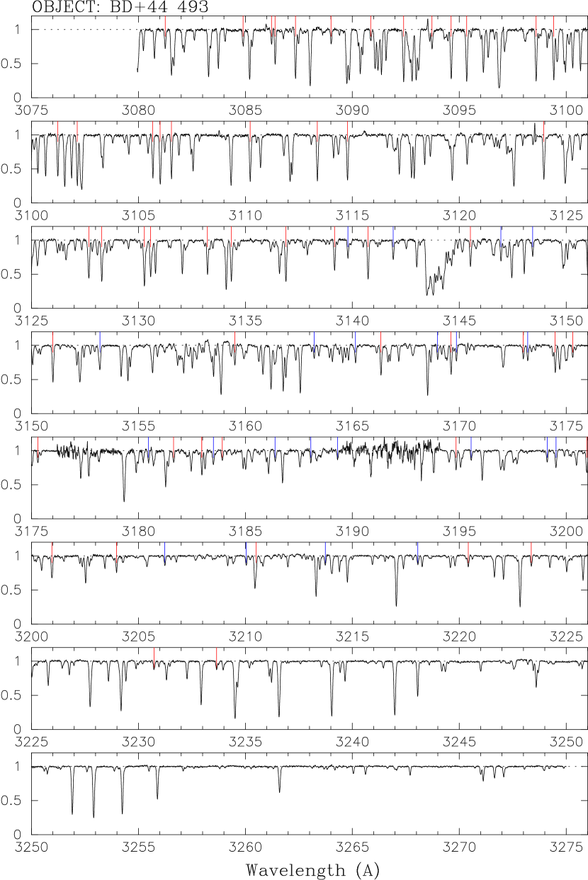
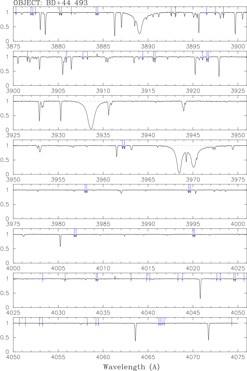
The extremely metal-poor (EMP) subgiant BD+44∘493 provides an excellent data-set of absorption lines that is useful to examine the 3D effects. This star was reported by Ito et al. (2009) as a carbon-enhanced object with extremely low metallicity ([Fe/H]). Detailed analysis of the spectrum of this object was recently reported by Ito et al. (2013) in which a spectral atlas is provided. The spectrum exhibits a number of clean CH and OH molecular lines. The apparent brightness of this object (the magnitude of 9.1) and appropriate effective temperature ( of 5430 K) make it possible to measure accurately individual molecular lines even for OH lines that appear around 3100 Å.
In this paper, we measure OH and CH molecular lines of BD+44∘493 and determine the oxygen and carbon abundances from individual spectral lines using 1D, static model atmospheres. We investigate the dependence of the derived abundances on excitation potentials of spectral lines as a test of 3D effects on this EMP star.
2 Observational data and line lists
The high resolution spectrum of BD+44∘493 analyzed in the present work was obtained with the High Dispersion Specrograph (HDS; Noguchi et al. 2002) of the Subaru Telescope. The data were studied by Ito et al. (2009, 2013) and the details on the observation are reported in these papers. The spectral resolution is that is sufficiently high for measurements of molecular lines. The signal-to-noise ratios (per pixel) around 3100 Å and 4000 Å, in which OH and CH molecular lines exist, are 100 and 400, respectively.
Examples of spectra of OH and CH systems are shown in Figures 1 and 2, respectively. We selected 99 OH lines and 105 CH lines for measurements of equivalent widths by Gaussian fitting. The line list of OH and CH, along with measured equivalent widths are given in Tables 1 and 2, respectively.
The line positions and excitation potentials of the OH 0–0, 1–1 and 2–2 systems are adopted from the line list compiled by Kurucz333http://kurucz.harvard.edu/molecules.html. The oscillator strengths (-values) in Table 1 are derived from the transition probabilities (-coefficient) of Luque & Crosley (1998) that are taken from LIFBASE444http://www.sri.com/engage/products-solutions/lifbase. The source of the transition probability is adopted in the compilation by Gillis et al. (2001) that has been used by previous studies on oxygen abundances of metal-poor stars based on OH lines (e.g., García Pérez et al. 2006; Frebel et al. 2008).
The line positions, excitation potentials, and transition probabilities of the CH 0–0 and 1–1 bands are taken from Masseron et al. (2014), who adopted the lifetimes measured by Luque & Crosley (1996a, b) to obtain the values. The -values are higher by 0.15 dex on average than those of Aoki et al. (2002) who adopted the values of the CH systems from Brown (1987).
3 Analysis and results
3.1 Abundance analysis based on 1D/LTE model atmospheres
3.2 OH lines
Figure 3 depicts the O abundances derived from individual OH lines as a function of their excitation potential. The results from different systems are shown by different symbols. The derived abundances exhibit a clear dependence on the excitation potential. A least square fit to the data points indicates the slope of dex/eV. A similar result is obtained even if the analysis is limited to the lines of the 0–0 system: the slope is dex/eV. The null hypothesis that there is no correlation between the two values is rejected by the regression analysis at the 99.9% confidence level. The slope derived from the 1–1 system is dex/eV. Although the correlation derived from the 1–1 system alone is slightly weaker, the confidence level is still 95% by the same analysis.
The correlation between the derived oxygen abundances and the excitation potentials is dependent on the adopted stellar parameters, in particular the effective temperature and the micro-turbulent velocity. If a lower effective temperature is adopted, the spectral lines with larger excitation potentials become weaker, resulting in higher abundances derived from these lines to explain the observed line absorption. Indeed, the slope in the diagram of the oxygen abundance and excitation potential is dex/eV for the analysis assuming K (Fig. 4b). Although the correlation is weaker than the that derived for the effective temperature we adopt ( K), it is still statistically significant. We note that the oxygen abundance derived for K on average is about 0.4 dex lower than that for K.
The slope is also dependent on the assumed micro-turbulent velocity. The micro-turbulent velocity is determined as the elemental abundances derived from individual lines show no dependence on the line strengths. The micro-turbulent velocity of this object, km s-1, is determined by the analysis of Fe I lines (Ito et al. 2013). Adopting this value, a correlation between the oxygen abundances and the strengths of OH lines is found (Fig. 4d). This is, however, attributed to the fact that lines with smaller excitation potential are stronger in general (Fig. 4f). There are four exceptionally weak lines () among those with small excitation potential ( eV). The oxygen abundances derived from these four lines are as high as the value obtained from stronger lines ((O) ), supporting our interpretation that the apparent correlation between the oxygen abundances and the strengths of OH lines is due to the dependence of the derived abundances on the excitation potentials of the OH lines. The slope obtained for km s-1 and K is (Fig. 4c).
We note for completeness that, although a weak correlation is found between the derived abundances and wavelengths of the lines (Fig. 4e), it is also explained by the fact that most of the lines with smaller excitation potential, from which higher abundances are derived, exist at shorter wavelengths.
3.3 CH lines
A similar analysis is made for CH lines as done for OH lines. The results are shown in Figure 5a. A clear correlation between the carbon abundances derived from individual CH lines and their excitation potentials is found as for OH lines. The null hypothesis that there is no correlation between the two values is rejected by the regression analysis at the 99.9% confidence level. The slope is dex/eV (Fig. 5a). The slope is slightly shallower, and dex/eV if larger micro-turbulent velocity ( km s-1) and lower effective temperature ( K), respectively, are adopted (Fig. 5b,c).
In the panels d and e of Figure 5, no clear correlation between the derived carbon abundances and wavelengths of CH lines, nor line strengths, is found. This would be due to the fact that the correlation between the wavelength and excitation potentials of CH lines is not as clear as of OH lines (Fig. 5f).
4 Discussion
4.1 OH and CH lines
Our 1D-LTE abundance analysis for OH and CH molecular lines for the extremely metal-poor star BD+44∘493 demonstrates that the derived oxygen and carbon abundances are dependent on the excitation potential with slopes of (dex/eV). This suggests that the spectral lines with smaller excitation potentials are enhanced by the existence of a cool layer in the atmosphere that is not reproduced by the current 1D models. 3D atmosphere models predict that the upper layer of photosphere is significantly cooler than that of the 1D models. Frebel et al. (2008) report the correction of oxygen and carbon abundances measured from OH and CH molecular lines using 3D model atmospheres as a function of excitation potentials. They estimate that the abundances derived from 3D models are lower than those from 1D models by dex and by dex for lines with and 1.0 dex, respectively. Namely, the 3D corrections explain the slopes of dex/eV found by our 1D analysis.
Dobrovolskas et al. (2013) also investigated line formation for molecules including OH and CH based on the 3D model atmospheres for red giants with 5000 K. Their models for [Fe/H] also predict similar trends of 3D corrections, as a function of excitation potentials, for these molecules that are similar to those of Frebel et al. (2008). More quantitatively, the correction for CH lines with shown in Figure 9 of Dobrovolskas et al. (2013) is smaller than those of Frebel et al. (2008). This difference might be partially due to the difference of the effective temperature and metallicity studied by the two works. The shallower slope found for CH than for OH in our result supports the prediction by Dobrovolskas et al. (2013).
4.2 Fe lines
A similar dependence of the derived abundances on excitation potentials of spectral lines is also expected for Fe lines. Collet et al. (2007) estimate that the correction reaches dex for low excitation lines of Fe I, and the slope could be about dex/eV for very metal-poor stars. Such a clear trend is, however, not found in our previous measurements of Fe lines (Figure 5 of Ito et al. 2013). A weaker trend, dex/eV, is found in the derived Fe abundances from Fe I lines. This trend, however, almost disappears if a slightly low is adopted in the analysis (Ito et al. 2013).
Figure 6 shows the Fe abundances derived from individual Fe I lines as functions of excitation potentials and equivalent widths. Large scatter is found in Fe abundances derived from lines with small excitation potentials shown by filled and open circles in the figure. Abundances from these lines show some dependence on line strengths: results from lines with equivalent widths larger than 80 mÅ exhibit lower abundances. Such trends suggest that spectral line formation is not well described by 1D LTE models.
The recent study by Dobrovolskas et al. (2013) predicts smaller corrections for Fe abundances derived from Fe I lines than that of Collet et al. (2007): their corrections are smaller than 0.2 dex for lines with eV. The correction for Fe abundances from Fe I lines with eV is, however, predicted to be still as large as 0.6 dex. The abundances derived from lines with eV for BD+44∘493 show scatter as large as 0.4 dex (Ito et al. 2013). The large scatter of abundances from low excitation Fe I lines might indicate that these lines are particularly affected by the 3D effect. These lines could also be affected by NLTE effects. Bergemann et al. (2012) conducted NLTE analyses for Fe lines of metal-poor stars using the spatial and temporal average stratification from 3D hydrodynamic models, as well as 1D static model atmospheres. They demonstrated for the cases of metal-poor stars like the subgiant HD 140283 that the analysis with the mean 3D models obtains lower Fe abundances on average, with smaller scatter of Fe abundances from individual Fe I lines, than those obtained from 1D models. On the other hand, the NLTE analysis using the 3D models derives higher Fe abundances than those obtained by a LTE analysis. If similar effects are working in the subgiant with lower metallicity like BD+44∘493, the averaged Fe abundances derived by the 1D LTE analysis is not significantly corrected by the 3D NLTE analysis, whereas the scatter found in abundances from individual lines with small excitation potentials becomes smaller.
We note that the Fe abundance obtained from Fe II lines by our analysis agrees well with that from Fe I lines even if we adopt the gravity () estimated adopting the parallax of this star to be 4.88 mas that is independent of the spectroscopic analysis of Fe lines (Ito et al. 2013). The NLTE and 3D effects estimated for Fe II lines are much smaller than those for neutral lines in general (Collet et al. 2007; Bergemann et al. 2012; Dobrovolskas et al. 2013). The agreement of Fe abundances obtained from lines of the two ionization stages using the 1D model suggests that the corrections by 3D NLTE analysis for Fe I lines is not as large as those estimated by 3D LTE models.
4.3 Carbon and oxygen abundances of BD+44∘493
The carbon and oxygen abundances of BD+44∘493 derived from the lines with relatively large excitation potentials () are (C)=5.8 and (O)=6.3, respectively (Fig. 5 and 4). Adopting the solar abundances (C)⊙=8.43 and (O)⊙=8.69 (Asplund et al. 2009) as well as [Fe/H] for BD+44∘493, the abundance ratios are [C/Fe] and [O/Fe]. The difference of oxygen abundances obtained from OH lines with (eV) by 3D and 1D model atmospheres () is approximately dex (Fig. 9 of Dobrovolskas et al. 2013). Similarly, the of carbon abundances from CH lines with and 1.0 (eV) are – dex. Including these corrections, [C/Fe] and [O/Fe] of BD+44∘493 are about 1.0 dex, indicating that carbon and oxygen are clearly enhanced in this object. We note that the C/O ratio obtained from CH and OH molecular lines estimated by 1D model atmospheres is robust.
The carbon abundance of BD+44∘493 is measured using the C I lines at 1.068–1.069 m by an NLTE analysis based on a 1D model atmosphere by Takeda & Takada-Hidai (2013), obtaining (C). This is slightly lower than the carbon abundance obtained from CH lines with 1D models, but agrees well with the value corrected for the 3D effects (see above). Takeda & Takada-Hidai (2013) mentioned, however, that the derived carbon abundance from the C I lines is sensitive to the treatment of NLTE effects. Hence, we cannot conclude that the estimate of the 3D effects for the carbon abundances from CH lines are quantitatively correct from the comparison with the carbon abundance from the C I lines. However, the agreement of the abundances within 0.1–0.2 dex from CH and C I lines is supportive for the reliable estimates of carbon abundance of this object.
5 Summary
BD+44∘493 is an extremely metal-poor subgiant with excesses of carbon and oxygen. Oxygen and carbon abundances derived from individual OH and CH lines by our analysis based on 1D LTE model atmospheres are dependent on the excitation potentials. This result might indicate existence of cool layer in the atmosphere which is not described by 1D models. Indeed, the dependence found for oxygen and carbon abundances on excitation potentials, dex/eV, is explained by the corrections estimated from 3D models.
While the behavior of Fe absorption lines is complicated, our analysis of OH and CH molecular lines qualitatively supports the prediction of the 3D models on the temperature structure of the surface atmosphere. For more quantitative discussion, investigations of the 3D models focusing on the stellar parameters of BD+44∘493 are desired.
References
- Aoki et al. (2002) Aoki, W., Norris, J. E., Ryan, S. G., Beers, T. C., & Ando, H. 2002, ApJ, 576, L141
- Asplund (2005) Asplund, M. 2005, ARA&A, 43, 481
- Asplund et al. (2003) Asplund, M., Carlsson, M., & Botnen, A. V. 2003, A&A, 399, L31
- Asplund et al. (2009) Asplund, M., Grevesse, N., Sauval, A. J., & Scott, P. 2009, ARA&A, 47, 481
- Asplund et al. (1999) Asplund, M., Nordlund, Å., Trampedach, R., & Stein, R. F. 1999, A&A, 346, L17
- Bergemann et al. (2012) Bergemann, M., Lind, K., Collet, R., Magic, Z., & Asplund, M. 2012, MNRAS, 427, 27
- Brown (1987) Brown, J. A. 1987, ApJ, 317, 701
- Castelli et al. (1997) Castelli, F., Gratton, R. G., & Kurucz, R. L. 1997, A&A, 318, 841
- Collet et al. (2007) Collet, R., Asplund, M., & Trampedach, R. 2007, A&A, 469, 687
- Dobrovolskas et al. (2013) Dobrovolskas, V., Kučinskas, A., Steffen, M., et al. 2013, A&A, 559, AA102
- García Pérez et al. (2006) García Pérez, A. E., Asplund, M., Primas, F., Nissen, P. E., & Gustafsson, B. 2006, A&A, 451, 621
- Gillis et al. (2001) Gillis, J. R., Goldman, A., Stark, G., & Rinsland, C. P. 2001, J. Quant. Spec. Radiat. Transf., 68, 225
- Gustafsson et al. (1975) Gustafsson, B., Bell, R. A., Eriksson, K., & Nordlund, A. 1975, A&A, 42, 407
- Frebel et al. (2008) Frebel, A., Collet, R., Eriksson, K., Christlieb, N., & Aoki, W. 2008, ApJ, 684, 588
- Ito et al. (2013) Ito, H., Aoki, W., Beers, T. C., et al. 2013, ApJ, 773, 33
- Ito et al. (2009) Ito, H., Aoki, W., Honda, S., & Beers, T. C. 2009, ApJ, 698, L37
- Kepa et al. (1996) Kepa, R., Para, A., Rytel, M., & Zachwieja, M. 1996, Journal of Molecular Spectroscopy, 178, 189
- Kurucz (1979) Kurucz, R. L. 1979, ApJS, 40, 1
- Masseron et al. (2014) Masseron, T., Plez, B., Van Eck, S., et al. 2014, A&A, 571, AA47
- Luque & Crosley (1996a) Luque, J., & Crosley, D. R. 1996a, J. Chem. Phys., 104, 2146
- Luque & Crosley (1996b) Luque, J., & Crosley, D. R. 1996b, J. Chem. Phys., 104, 3907
- Luque & Crosley (1998) Luque, J., & Crosley, D. R. 1998, J. Chem. Phys., 109, 439
- Noguchi et al. (2002) Noguchi, K. et al. 2002, PASJ, 54, 855
- Takeda & Takada-Hidai (2013) Takeda, Y., & Takada-Hidai, M. 2013, PASJ, 65, 65


| Wavelength (Å) | (eV) | (mÅ) | |
|---|---|---|---|
| OH 0–0 system | |||
| 3081.254 | 0.762 | -1.882 | 21.1 |
| 3084.048 | 0.016 | -3.162 | 12.6 |
| 3084.895 | 0.843 | -1.874 | 18.8 |
| 3086.224 | 0.925 | -1.852 | 14.4 |
| 3086.391 | 0.010 | -2.482 | 37.0 |
| 3087.342 | 0.095 | -1.896 | 58.9 |
| 3089.008 | 0.928 | -1.869 | 15.0 |
| 3090.862 | 1.013 | -1.850 | 12.8 |
| 3092.397 | 0.164 | -1.782 | 65.5 |
| 3093.724 | 0.016 | -2.860 | 24.6 |
| 3094.619 | 0.134 | -1.899 | 63.4 |
| 3095.344 | 0.205 | -1.738 | 64.9 |
| 3095.545 | 0.205 | -3.121 | 7.6 |
| 3096.650 | 0.170 | -3.098 | 11.4 |
| 3098.589 | 0.250 | -1.700 | 63.3 |
| 3099.414 | 0.210 | -1.788 | 65.7 |
| 3101.230 | 0.067 | -2.205 | 48.0 |
| 3102.144 | 0.300 | -1.667 | 66.5 |
| 3104.351 | 1.202 | -1.868 | 10.4 |
| 3105.666 | 0.304 | -1.708 | 47.6 |
| 3106.019 | 0.354 | -1.639 | 65.4 |
| 3106.546 | 0.095 | -2.142 | 49.2 |
| 3107.855 | 1.297 | -1.858 | 6.0 |
| 3110.226 | 0.412 | -1.615 | 56.8 |
| 3110.530 | 1.300 | -1.873 | 9.9 |
| 3113.365 | 0.415 | -1.649 | 55.3 |
| 3114.773 | 0.474 | -1.594 | 54.5 |
| 3123.948 | 0.205 | -2.003 | 58.0 |
| 3127.687 | 0.612 | -1.589 | 51.7 |
| 3128.286 | 0.210 | -2.074 | 56.6 |
| 3130.281 | 0.250 | -1.969 | 65.4 |
| 3130.570 | 0.683 | -1.549 | 52.7 |
| 3133.228 | 0.686 | -1.575 | 44.1 |
| 3134.344 | 0.255 | -2.031 | 54.0 |
| 3136.895 | 0.299 | -1.939 | 51.0 |
| 3139.169 | 0.763 | -1.564 | 34.0 |
| 3140.506 | 0.304 | -3.041 | 6.7 |
| 3140.734 | 0.304 | -1.994 | 46.0 |
| 3145.520 | 0.845 | -1.555 | 31.5 |
| 3151.003 | 0.411 | -1.890 | 42.0 |
| 3159.505 | 1.017 | -1.545 | 21.7 |
| 3166.337 | 0.538 | -1.853 | 35.3 |
| 3169.613 | 0.542 | -1.891 | 32.7 |
| 3172.992 | 1.202 | -1.526 | 16.2 |
| 3174.483 | 0.608 | -1.839 | 37.2 |
| 3175.301 | 1.204 | -1.545 | 13.8 |
| 3181.646 | 1.300 | -1.530 | 14.4 |
| 3182.962 | 0.682 | -1.827 | 28.5 |
| 3183.921 | 1.302 | -1.549 | 13.6 |
| 3194.847 | 0.762 | -1.848 | 23.7 |
| 3200.488 | 1.505 | -1.546 | 20.0 |
| 3200.959 | 0.840 | -1.810 | 28.0 |
| 3203.975 | 0.843 | -1.839 | 20.4 |
| 3210.500 | 0.925 | -1.805 | 49.8 |
| 3220.418 | 1.013 | -1.802 | 14.5 |
| 3223.366 | 1.016 | -1.828 | 11.5 |
| 3223.731 | 1.723 | -1.588 | 3.6 |
| 3230.729 | 1.104 | -1.802 | 9.9 |
| 3233.654 | 1.107 | -1.826 | 10.9 |
| 3241.448 | 1.199 | -1.803 | 8.1 |
| 3252.594 | 1.297 | -1.807 | 5.8 |
| 3255.492 | 1.300 | -1.829 | 5.2 |
| 3264.185 | 1.398 | -1.813 | 4.0 |
| OH 1–1 system | |||
| 3122.962 | 0.507 | -2.555 | 10.3 |
| 3127.042 | 0.571 | -2.442 | 10.5 |
| 3127.353 | 0.735 | -2.269 | 10.8 |
| 3128.060 | 0.541 | -2.511 | 21.2 |
| 3128.518 | 0.786 | -2.242 | 16.3 |
| 3129.538 | 0.516 | -2.597 | 9.3 |
| 3136.178 | 0.452 | -2.570 | 17.9 |
| 3139.794 | 0.485 | -2.279 | 20.4 |
| 3141.911 | 0.507 | -2.186 | 22.0 |
| 3146.947 | 0.565 | -2.052 | 24.5 |
| 3148.430 | 0.516 | -2.277 | 17.6 |
| 3153.204 | 0.640 | -1.960 | 36.9 |
| 3163.215 | 0.534 | -2.351 | 14.8 |
| 3165.150 | 0.783 | -1.871 | 21.5 |
| 3168.983 | 0.565 | -2.298 | 16.1 |
| 3169.174 | 0.541 | -2.472 | 9.3 |
| 3169.866 | 0.838 | -1.851 | 17.6 |
| 3173.198 | 0.842 | -1.885 | 18.0 |
| 3180.472 | 0.961 | -1.822 | 15.2 |
| 3183.510 | 0.965 | -1.851 | 20.1 |
| 3186.389 | 1.028 | -1.812 | 13.7 |
| 3188.062 | 0.683 | -2.182 | 12.1 |
| 3189.311 | 1.032 | -1.840 | 9.7 |
| 3195.555 | 1.102 | -1.832 | 12.6 |
| 3199.108 | 0.735 | -2.209 | 12.9 |
| 3199.523 | 1.174 | -1.803 | 22.7 |
| 3206.235 | 0.786 | -2.180 | 10.6 |
| 3206.771 | 1.252 | -1.804 | 7.2 |
| 3210.042 | 0.837 | -2.110 | 10.8 |
| 3213.738 | 0.842 | -2.155 | 11.7 |
| 3218.061 | 0.897 | -2.093 | 10.1 |
| 3229.891 | 0.964 | -2.118 | 8.9 |
| 3238.552 | 1.031 | -2.104 | 6.6 |
| 3240.750 | 1.597 | -1.836 | 3.8 |
| 3253.875 | 1.172 | -2.057 | 6.1 |
| 3263.826 | 1.250 | -2.055 | 3.2 |
| OH 2–2 system | |||
| 3206.518 | 0.953 | -2.387 | 4.2 |
| 3221.127 | 1.059 | -2.295 | 3.9 |
| Wavelength (Å) | (eV) | (mÅ) | |
|---|---|---|---|
| CH system | |||
| 3871.363 | 0.098 | -1.68 | 8.8 |
| 3873.557 | 0.035 | -1.94 | 5.9 |
| 3874.543 | 0.191 | -1.55 | 10.0 |
| 3874.782 | 0.191 | -1.51 | 10.5 |
| 3875.311 | 0.021 | -2.08 | 5.1 |
| 3876.980 | 0.229 | -1.51 | 9.5 |
| 3877.193 | 0.229 | -1.49 | 10.1 |
| 3877.467 | 0.010 | -2.30 | 3.1 |
| 3880.186 | 0.270 | -1.49 | 8.9 |
| 3880.387 | 0.270 | -1.47 | 9.8 |
| 3881.478 | 0.004 | -2.30 | 3.5 |
| 3884.225 | 0.314 | -1.47 | 9.1 |
| 3884.414 | 0.314 | -1.45 | 10.2 |
| 3892.585 | 0.035 | -1.58 | 12.8 |
| 3893.064 | 0.035 | -1.49 | 16.6 |
| 3896.530 | 0.010 | -2.08 | 5.2 |
| 3897.480 | 0.011 | -1.93 | 7.4 |
| 3898.389 | 0.074 | -1.35 | 19.4 |
| 3901.591 | 0.098 | -1.35 | 17.7 |
| 3905.902 | 0.126 | -1.25 | 20.8 |
| 3907.766 | 0.035 | -1.82 | 8.6 |
| 3908.268 | 0.035 | -1.74 | 9.6 |
| 3914.419 | 0.053 | -1.67 | 10.7 |
| 3915.609 | 0.192 | -1.22 | 20.3 |
| 3915.790 | 0.192 | -1.18 | 22.4 |
| 3921.072 | 0.074 | -1.61 | 13.6 |
| 3962.173 | 0.229 | -1.46 | 10.8 |
| 3962.389 | 0.229 | -1.43 | 11.9 |
| 3983.001 | 0.314 | -1.41 | 9.7 |
| 3983.191 | 0.314 | -1.39 | 10.2 |
| 3994.501 | 0.361 | -1.39 | 9.6 |
| 3994.691 | 0.361 | -1.38 | 10.1 |
| 4006.805 | 0.411 | -1.38 | 8.2 |
| 4006.994 | 0.412 | -1.37 | 8.3 |
| 4020.020 | 0.465 | -1.37 | 7.7 |
| 4020.186 | 0.465 | -1.36 | 8.2 |
| 4034.234 | 0.521 | -1.36 | 6.7 |
| 4038.113 | 0.349 | -2.14 | 1.8 |
| 4039.860 | 0.359 | -2.14 | 1.7 |
| 4043.332 | 0.372 | -2.02 | 2.3 |
| 4043.825 | 0.373 | -1.93 | 3.5 |
| 4047.667 | 0.389 | -1.93 | 2.5 |
| 4049.555 | 0.580 | -1.36 | 0.0 |
| 4049.715 | 0.580 | -1.36 | 6.3 |
| 4050.685 | 0.359 | -2.35 | 1.4 |
| 4051.358 | 0.359 | -2.25 | 1.5 |
| 4052.936 | 0.410 | -1.87 | 3.1 |
| 4053.263 | 0.410 | -1.81 | 3.8 |
| 4059.206 | 0.433 | -1.82 | 3.0 |
| 4059.484 | 0.433 | -1.78 | 3.5 |
| 4066.800 | 0.460 | -1.75 | 3.3 |
| 4074.320 | 0.409 | -2.11 | 1.8 |
| 4075.112 | 0.490 | -1.75 | 3.4 |
| 4075.320 | 0.490 | -1.74 | 3.7 |
| 4084.001 | 0.433 | -2.06 | 1.6 |
| 4094.682 | 0.460 | -2.02 | 2.1 |
| 4106.456 | 0.490 | -1.99 | 1.9 |
| 4106.713 | 0.490 | -1.97 | 2.0 |
| 4119.432 | 0.523 | -1.97 | 1.9 |
| 4119.669 | 0.523 | -1.96 | 1.5 |
| CH system | |||
| 4153.408 | 1.234 | -1.16 | 1.4 |
| 4153.634 | 1.234 | -1.17 | 1.5 |
| 4158.012 | 1.152 | -1.17 | 1.7 |
| 4162.464 | 1.072 | -1.17 | 2.4 |
| 4162.667 | 1.072 | -1.18 | 2.3 |
| 4172.513 | 0.919 | -1.19 | 3.7 |
| 4177.834 | 0.847 | -1.21 | 4.1 |
| 4177.997 | 0.847 | -1.22 | 4.0 |
| 4183.330 | 0.777 | -1.22 | 4.7 |
| 4183.472 | 0.777 | -1.23 | 4.8 |
| 4253.000 | 0.523 | -1.51 | 5.1 |
| 4253.206 | 0.523 | -1.47 | 5.7 |
| 4255.248 | 0.157 | -1.46 | 14.4 |
| 4255.628 | 0.157 | -1.50 | 13.8 |
| 4255.823 | 0.157 | -1.46 | 14.9 |
| 4259.087 | 0.490 | -1.54 | 4.8 |
| 4259.282 | 0.490 | -1.50 | 5.6 |
| 4261.218 | 0.125 | -1.54 | 13.4 |
| 4261.521 | 0.126 | -1.49 | 15.8 |
| 4261.731 | 0.126 | -1.54 | 14.4 |
| 4261.982 | 0.126 | -1.49 | 15.5 |
| 4263.969 | 0.460 | -1.57 | 4.8 |
| 4264.265 | 0.460 | -1.53 | 6.0 |
| 4264.466 | 0.460 | -1.57 | 6.3 |
| 4264.711 | 0.460 | -1.53 | 7.1 |
| 4274.186 | 0.074 | -1.56 | 14.5 |
| 4276.083 | 0.807 | -1.58 | 1.5 |
| 4277.010 | 1.152 | -0.93 | 3.2 |
| 4277.230 | 1.152 | -0.94 | 3.2 |
| 4278.855 | 1.072 | -0.94 | 3.8 |
| 4279.055 | 1.072 | -0.95 | 4.2 |
| 4279.480 | 0.052 | -1.67 | 11.7 |
| 4282.787 | 0.919 | -0.97 | 6.5 |
| 4286.886 | 0.777 | -1.00 | 9.0 |
| 4287.036 | 0.777 | -1.01 | 9.3 |
| 4343.173 | 0.073 | -2.14 | 4.0 |
| 4343.489 | 0.074 | -2.14 | 4.6 |
| 4343.687 | 0.074 | -2.05 | 5.2 |
| 4343.963 | 0.074 | -2.05 | 5.1 |
| 4347.538 | 0.098 | -2.02 | 5.5 |
| 4348.336 | 0.098 | -1.95 | 6.3 |
| 4355.341 | 0.490 | -1.84 | 3.0 |
| 4355.693 | 0.157 | -1.85 | 6.5 |
| 4355.992 | 0.157 | -1.79 | 8.0 |
| 4356.355 | 0.157 | -1.85 | 7.5 |
| 4356.594 | 0.157 | -1.79 | 7.4 |