Asymptotic Mutual Information for the
Two-Groups Stochastic Block Model

Abstract

We develop an information-theoretic view of the stochastic block model, a popular statistical model for the large-scale structure of complex networks. A graph $G$ from such a model is generated by first assigning vertex labels at random from a finite alphabet, and then connecting vertices with edge probabilities depending on the labels of the endpoints. In the case of the symmetric two-group model, we establish an explicit ‘single-letter’ characterization of the per-vertex mutual information between the vertex labels and the graph.

The explicit expression of the mutual information is intimately related to estimation-theoretic quantities, and –in particular– reveals a phase transition at the critical point for community detection. Below the critical point the per-vertex mutual information is asymptotically the same as if edges were independent. Correspondingly, no algorithm can estimate the partition better than random guessing. Conversely, above the threshold, the per-vertex mutual information is strictly smaller than the independent-edges upper bound. In this regime there exists a procedure that estimates the vertex labels better than random guessing.

1 Introduction and main results

The stochastic block model is the simplest statistical model for networks with a community (or cluster) structure. As such, it has attracted considerable amount of work across statistics, machine learning, and theoretical computer science [HLL83, DF89, SN97, CK99, ABFX08]. A random graph ${\boldsymbol{G}}=(V,E)$ from this model has its vertex set $V$ partitioned into $r$ groups, which are assigned $r$ distinct labels. The probability of edge $(i,j)$ being present depends on the group labels of vertices $i$ and $j$.

In the context of social network analysis, groups correspond to social communities [HLL83]. For other data-mining applications, they represent latent attributes of the nodes [McS01]. In all of these cases, we are interested in inferring the vertex labels from a single realization of the graph.

In this paper we develop an information-theoretic viewpoint on the stochastic block model. Namely, we develop an explicit (‘single-letter’) expression for the per-vertex conditional entropy of the vertex labels given the graph. Equivalently, we compute the asymptotic per-vertex mutual information between the graph and the vertex labels. Our results hold asymptotically for large networks under suitable conditions on the model parameters. The asymptotic mutual information is of independent interest, but is also intimately related to estimation-theoretic quantities.

For the sake of simplicity, we will focus on the symmetric two group model. Namely, we assume the vertex set $V=[n]\equiv\{1,2,\dots,n\}$ to be partitioned into two sets $V=V_{+}\cup V_{-}$, with ${\mathbb{P}}(i\in V_{+})={\mathbb{P}}(i\in V_{-})=1/2$ independently across vertices $i$. In particular, the size of each group $|V_{+}|,|V_{-}|\sim{\rm Binom}(n,1/2)$ concentrates tightly around its expectation $n/2$. Conditional on the edge labels, edges are independent with

$${\mathbb{P}}\big{(}(i,j)\in E\big{|}V_{+},V_{-}\big{)}=\begin{cases}p_{n}&\mbox{ if $\{i,j\}\subseteq V_{+}$, or $\{i,j\}\subseteq V_{-}$,}\\ q_{n}&\mbox{ otherwise.}\\ \end{cases}$$ (1)

Throughout we will denote by ${\boldsymbol{X}}=(X_{i})_{i\in V}$ the set of vertex labels $X_{i}\in\{+1,-1\}$, and we will be interested in the conditional entropy $H({\boldsymbol{X}}|{\boldsymbol{G}})$ or –equivalently– the mutual information $I({\boldsymbol{X}};{\boldsymbol{G}})$ in the limit $n\to\infty$. We will write ${\boldsymbol{G}}\sim{\rm SBM}(n;p,q)$ (or $({\boldsymbol{X}},{\boldsymbol{G}})\sim{\rm SBM}(n;p,q)$) to imply that the graph $G$ is distributed according to the stochastic block model with $n$ vertices and parameters $p,q$.

Since we are interested in the large $n$ behavior, two preliminary remarks are in order:

1. Normalization. We obviously have $0\leq H({\boldsymbol{X}}|{\boldsymbol{G}})\leq n\,\log 2$. It is therefore natural to study the per-vertex entropy $H({\boldsymbol{X}}|{\boldsymbol{G}})/n$.

   As we will see, depending on the model parameters, this will take any value between $0$ and $\log 2$.

2. Scaling. The reconstruction problem becomes easier when $p_{n}$ and $q_{n}$ are well separated, and more difficult when they are closer to each other. For instance, in an early contribution, Dyer and Frieze [DF89] proved that the labels can be reconstructed exactly –modulo an overall flip– if $p_{n}=p>q_{n}=q$ are distinct and independent of $n$. This –in particular– implies $H({\boldsymbol{X}}|{\boldsymbol{G}})/n\to 0$ in this limit (in fact, it implies $H({\boldsymbol{X}}|{\boldsymbol{G}})\to\log 2$). In this regime, the ‘signal’ is so strong that the conditional entropy is trivial. Indeed, recent work [ABH14, MNS14a] show that this can also happen with $p_{n}$ and $q_{n}$ vanishing, and characterizes the sequences $(p_{n},q_{n})$ for which this happens. (See Section 2 for an account of related work.)

   Let $\overline{p}_{n}=(p_{n}+q_{n})/2$ be the average edge probability. It turns out that the relevant ‘signal-to-noise ratio’ (SNR) is given by the following parameter:

   $$\lambda_{n}=\frac{n\,(p_{n}-q_{n})^{2}}{4\overline{p}_{n}(1-\overline{p}_{n})}\,.$$ (2)

   Indeed, we will see that $H({\boldsymbol{X}}|{\boldsymbol{G}})/n$ of order $1$, and has a strictly positive limit when $\lambda_{n}$ is of order one. This is also the regime in which the fraction of incorrectly labeled vertices has a limit that is strictly between $0$ and $1$.

1.1 Main result: Asymptotic per-vertex mutual information

As mentioned above, our main result provides a single-letter characterization for the per-vertex mutual information. This is given in terms of an effective Gaussian scalar channel. Namely, define the Gaussian channel

$$Y_{0}=Y_{0}(\gamma)=\sqrt{\gamma}\,X_{0}+Z_{0},$$ (3)

where $X_{0}\sim{\rm Uniform}(\{+1,-1\})$ independent of $Z_{0}\sim{\sf N}(0,1)$. We denote by ${\sf mmse}(\gamma)$ and ${\sf I}(\gamma)$ the corresponding minimum mean square error and mutual information:

$${\sf I}(\gamma) ={\mathbb{E}}\,\log\Big{\{}\frac{{\rm d}p_{Y|X}(Y_{0}(\gamma)|X_{0})}{{\rm d}p_{Y}(Y_{0}(\gamma))}\Big{\}}\,,$$ (4)

$${\sf mmse}(\gamma) ={\mathbb{E}}\left\{(X_{0}-{\mathbb{E}}\left\{X_{0}|Y_{0}(\gamma)\right\})^{2}\right\}\,.$$ (5)

In the present case, these quantities can be written explicitly as Gaussian integrals of elementary functions:

$${\sf I}(\gamma) =\gamma-{\mathbb{E}}\log\cosh\big{(}\gamma+\sqrt{\gamma}\,Z_{0}\big{)}\,,$$ (6)

$${\sf mmse}(\gamma) =1-{\mathbb{E}}\big{\{}\tanh(\gamma+\sqrt{\gamma}\,Z_{0})^{2}\big{\}}\,.$$ (7)

We are now in position to state our main result.

Theorem 1.1.

For any $\lambda>0$, let $\gamma_{*}=\gamma_{*}(\lambda)$ be the largest non-negative solution of the equation:

$$\gamma =\lambda\big{(}1-{\sf mmse}(\gamma)\big{)}\,.$$ (8)

We refer to $\gamma_{*}(\lambda)$ as to the effective signal-to-noise ratio. Further, define $\Psi(\gamma,\lambda)$ by:

$$\Psi(\gamma,\lambda) =\frac{\lambda}{4}+\frac{\gamma^{2}}{4\lambda}-\frac{\gamma}{2}+{\sf I}(\gamma)\,.$$ (9)

Let the graph ${\boldsymbol{G}}$ and vertex labels ${\boldsymbol{X}}$ be distributed according to the stochastic block model with $n$ vertices and parameters $p_{n},q_{n}$ (i.e. $({\boldsymbol{G}},{\boldsymbol{X}})\sim{\rm SBM}(n;p_{n},q_{n})$) and define $\lambda_{n}\equiv n\,(p_{n}-q_{n})^{2}/(4\overline{p}_{n}(1-\overline{p}_{n}))$.

Assume that, as $n\to\infty$, $(i)$ $\lambda_{n}\to\lambda$ and $(ii)$ $n\overline{p}_{n}(1-\overline{p}_{n})\to\infty$. Then,

$$\lim_{n\to\infty}\frac{1}{n}\,I({\boldsymbol{X}};{\boldsymbol{G}}) =\Psi(\gamma_{*}(\lambda),\lambda)\,.$$ (10)

A few remarks are in order.

Remark 1.2.

Of course, we could have stated our result in terms of conditional entropy. Namely

$$\lim_{n\to\infty}\frac{1}{n}\,H({\boldsymbol{X}}|{\boldsymbol{G}}) =\log 2-\Psi(\gamma_{*}(\lambda),\lambda)\,.$$ (11)

Remark 1.3.

Notice that our assumptions require $n\overline{p}_{n}(1-\overline{p}_{n})\to\infty$ at any, arbitrarily slow, rate. In words, this corresponds to the graph average degree diverging at any, arbitrarily slow, rate.

Recently (see Section 2 for a discussion of this literature), there has been considerable interest in the case of bounded average degree, namely

$$p_{n}=\frac{a}{n}\,,\;\;\;\;\;\;q_{n}=\frac{b}{n}\,,$$ (12)

with $a,b$ bounded. Our proof gives an explicit error bound in terms of problem parameters even when $n\overline{p}_{n}(1-\overline{p}_{n})$ is of order one. Hence we are able to characterize the asymptotic mutual information for large-but-bounded average degree up to an offset that vanishes with the average degree.

Explicitly, we prove that:

$$\limsup_{n\to\infty}\Big{|}\frac{1}{n}I({\boldsymbol{X}};{\boldsymbol{G}})-\Psi(\gamma_{*}(\lambda),\lambda)\Big{|}\leq\frac{C\lambda^{3}}{\sqrt{a+b}}\,,$$ (13)

for some absolute constant $C$.

Our main result and its proof has implications on the minimum error that can be achieved in estimating the labels ${\boldsymbol{X}}$ from the graph ${\boldsymbol{G}}$. For reasons that will become clear below, a natural metric is given by the matrix minimum mean square error

$${\sf MMSE}_{n}(\lambda) \equiv\frac{1}{n(n-1)}{\mathbb{E}}\Big{\{}\big{\|}{\boldsymbol{X}}{\boldsymbol{X}}^{{\sf T}}-{\mathbb{E}}\{{\boldsymbol{X}}{\boldsymbol{X}}^{{\sf T}}|{\boldsymbol{G}}\}\big{\|}_{F}^{2}\Big{\}}\,.$$ (14)

(Occasionally, we will also use the notation ${\sf MMSE}(\lambda;n)$ for ${\sf MMSE}_{n}(\lambda)$.) Using the exchangeability of the indices $\{1,\dots,n\}$, this can also be rewritten as

$${\sf MMSE}_{n}(\lambda) =\frac{2}{n(n-1)}\sum_{1\leq i<j\leq n}{\mathbb{E}}\big{\{}\big{[}X_{i}X_{j}-{\mathbb{E}}\{X_{i}X_{j}|{\boldsymbol{G}}\}\big{]}^{2}\big{\}}$$ (15)

$$={\mathbb{E}}\big{\{}\big{[}X_{1}X_{2}-{\mathbb{E}}\{X_{1}X_{2}|{\boldsymbol{G}}\}\big{]}^{2}\big{\}}$$ (16)

$$=\min_{\widehat{x}_{12}:\mathcal{G}_{n}\to\mathbb{R}}{\mathbb{E}}\big{\{}\big{[}X_{1}X_{2}-\widehat{x}_{12}({\boldsymbol{G}})\big{]}^{2}\big{\}}\,.$$ (17)

(Here $\mathcal{G}_{n}$ denotes the set of graphs with vertex set $[n]$.) In words, ${\sf MMSE}_{n}(\lambda)$ is the minimum error incurred in estimating the relative sign of the labels of two given (distinct) vertices. Equivalently, we can assume that vertex $1$ has label $X_{1}=+1$. Then ${\sf MMSE}_{n}(\lambda)$ is the minimum mean square error incurred in estimating the label of any other vertex, say vertex $2$. Namely, by symmetry, we have (see Section 3)

$${\sf MMSE}_{n}(\lambda) ={\mathbb{E}}\big{\{}\big{[}X_{2}-{\mathbb{E}}\{X_{2}|X_{1}=+1,{\boldsymbol{G}}\}\big{]}^{2}\big{|}X_{1}=+1\big{\}}$$ (18)

$$=\min_{\widehat{x}_{2|1}:\mathcal{G}_{n}\to\mathbb{R}}{\mathbb{E}}\big{\{}\big{[}X_{2}-\widehat{x}_{2|1}({\boldsymbol{G}})\big{]}^{2}|X_{1}=+1\big{\}}\,.$$ (19)

In particular ${\sf MMSE}_{n}(\lambda)\in[0,1]$, with ${\sf MMSE}_{n}(\lambda)\to 1$ corresponding to random guessing.

Theorem 1.4.

Under the assumptions of Theorem 1.1 (in particular assuming $\lambda_{n}\to\lambda$ as $n\to\infty$), the following limit holds for the matrix minimum mean square error

$$\lim_{n\to\infty}{\sf MMSE}_{n}(\lambda_{n})=1-\frac{\gamma_{*}(\lambda)^{2}}{\lambda^{2}}\,.$$ (20)

Further, this implies $\lim_{n\to\infty}{\sf MMSE}_{n}(\lambda_{n})=1$ for $\lambda\leq 1$ and $\lim_{n\to\infty}{\sf MMSE}_{n}(\lambda_{n})<1$ for $\lambda>1$.

For further discussion of this result and its generalizations, we refer to Section 3. In particular, Corollary 3.7 establishes that $\lambda=1$ is a phase transition for other estimation metrics as well, in particular for overlap and vector mean square error.

Remark 1.5.

As Theorem 1.1, also the last theorem holds under the mild condition that the average degree $n\overline{p}_{n}$ diverges at any, arbitrarily slow rate. This should be contrasted with the phase transition of naive spectral methods.

It is well understood that the community structure can be estimated by the principal eigenvector of the centered adjacency matrix ${\boldsymbol{G}}-{\mathbb{E}}\{{\boldsymbol{G}}\}=({\boldsymbol{G}}-\overline{p}_{n}{\mathbf{1}}{\mathbf{1}}^{{\sf T}})$. (We denote by ${\boldsymbol{G}}$ the graph as well as its adjacency matrix.) This approach is successful fro $\lambda>1$ but requires average degree $n\overline{p}_{n}\geq(\log n)^{c}$ for $c$ a constant [CDMF09, BGN11].

Remark 1.6.

Our proof of Theorem 1.1 and Theorem 1.4 involves the analysis of a Gaussian observation model, whereby the rank one matrix ${\boldsymbol{X}}{\boldsymbol{X}}^{{\sf T}}$ is corrupted by additive Gaussian noise, according to ${\boldsymbol{Y}}=\sqrt{\lambda/n}{\boldsymbol{X}}{\boldsymbol{X}}^{\sf T}+{\boldsymbol{Z}}$. In particular, we prove a single letter characterization of the asymptotic mutual information per dimension in this model $\lim_{n\to\infty}I({\boldsymbol{X}};{\boldsymbol{Y}})$, cf. Theorem 4.3 below. The resulting asymptotic value is proved to coincide with the asymptotic value in the stochastic block model, as established in Theorem 1.1. In other words, the per-dimension mutual information turns out to be universal across multiple noise models.

1.2 Outline of the paper

In Section 2 we review the literature on this problem. We then discuss the connection with estimation in Section 3. This section also demonstrates how to evaluate the asymptotic formula in Theorem 1.1.

Section 4 describes the proof strategy. As an intermediate step, we introduce a Gaussian observation model which is of independent interest. The proof of Theorem 1.1 is reduced to two main propositions:

• Proposition 4.1 establishes that –within the regime defined in Theorem 1.1– the stochastic block model is asymptotically equivalent to the Gaussian observation model (see Section 4 for a formal definition). This statement (with explicit error bounds) is proved in Section 5 through a careful application of the Lindeberg method.

• Proposition 4.2 develops a single-letter characterization of the asymptotic per-vertex mutual information of the Gaussian observation model. The proof of this fact is presented in Section 6 and builds on two steps. We first prove an asymptotic upper bound on the matrix minimum mean square error ${\sf MMSE}_{n}(\lambda)$ using an approximate message passing (AMP) algorithm. We then use an area theorem to prove that this upper bound is tight.

Finally, Section 7 contains the proof of Theorem 1.4. Several technical details are deferred to the appendices.

1.3 Notations

The set of first $n$ integers is denoted by $[n]=\{1,2,\dots,n\}$.

When possible, we will follow the convention of denoting random variables by upper-case letters (e.g. $X,Y,Z,\dots$), and their values by lower case letters (e.g. $x,y,z,\dots$). We use boldface for vectors and matrices, e.g. ${\boldsymbol{X}}$ for a random vector and ${\boldsymbol{x}}$ for a deterministic vector. The graph ${\boldsymbol{G}}$ will be identified with its adjacency matrix. Namely, with a slight abuse of notation, we will use ${\boldsymbol{G}}$ both to denote a graph ${\boldsymbol{G}}=(V=[n],E)$ (with $V=[n]$ the vertex set, and $E$ the edge set, i.e. a set of unordered pairs of vertices), and its adjacency matrix. This is a symmetric zero-one matrix ${\boldsymbol{G}}=(G_{ij})_{1\leq i,j\leq n}$ with entries

$$G_{ij}=\begin{cases}1&\;\mbox{if $(i,j)\in E$},\\ 0&\;\mbox{otherwise.}\end{cases}$$ (21)

Throughout we assume $G_{ii}=0$ by convention.

We write $f_{1}(n)=f_{2}(n)+O(f_{3}(n))$ to mean that $\left\lvert{f_{1}(n)-f_{2}(n)}\right\rvert\leq Cf_{3}(n)$ for a universal constant $C$. We denote by $C$ a generic (large) constant that is independent of problem parameters, whose value can change from line to line.

We say that an event holds with high probability if it holds with probability converging to one as $n\to\infty$.

We denote the $\ell_{2}$ norm of a vector ${\boldsymbol{x}}$ by $\left\lVert{{\boldsymbol{x}}}\right\rVert_{2}$ and the Frobenius norm of a matrix ${\boldsymbol{Y}}$ by $\left\lVert{{\boldsymbol{Y}}}\right\rVert_{F}$. The ordinary scalar product of vectors ${\boldsymbol{a}},{\boldsymbol{b}}\in\mathbb{R}^{m}$ is denoted as $\langle{\boldsymbol{a}},{\boldsymbol{b}}\rangle\equiv\sum_{i=1}^{m}a_{i}b_{i}$.

Unless stated otherwise, logarithms will be taken in the natural basis, and entropies measured in nats.

2 Related work

The stochastic block model was first introduced within the social science literature in [HLL83]. Around the same time, it was studied within theoretical computer science [BCLS87, DF89], under the name of ‘planted partition model. ’

A large part of the literature has focused on the problem of exact recovery of the community (cluster) structure. A long series of papers [BCLS87, DF89, Bop87, SN97, JS98, CK99, CI01, McS01, BC09, RCY11, CWA12, CSX12, Vu14, YC14], establishes sufficient conditions on the gap between $p_{n}$ and $q_{n}$ that guarantee exact recovery of the vertex labels with high probability. A sharp threshold for exact recovery was obtained in [ABH14, MNS14a], showing that for $p_{n}=\alpha\log(n)/n$, $q_{n}=\beta\log(n)/n$, $\alpha,\beta>0$, exact recovery is solvable (and efficiently so) if and only if $\sqrt{\alpha}-\sqrt{\beta}\geq 2$. Efficient algorithms for this problem were also developed in [YP14, BH14, Ban15]. For the SBM with arbitrarily many communities, necessary and sufficient conditions for exact recovery were recently obtained in [AS15]. The resulting sharp threshold is efficiently achievable and is stated in terms of a CH-divergence.

A parallel line of work studied the detection problem. In this case, the estimated community structure is only required to be asymptotically positively correlated with the ground truth. For this requirement, two independent groups [Mas14, MNS14b] proved that detection is solvable (and so efficiently) if and only if $(a-b)^{2}>2(a+b)$, when $p_{n}=a/n$, $q_{n}=b/n$. This settles a conjecture made in [DKMZ11] and improves on earlier work [Co10]. Results for detection with more than two communities were recently obtained in [GV14, CRV15, AS15, BLM15]. A variant of community detection with a single hidden community in a sparse graph was studied in [Mon15].

In a sense, the present paper bridges detection and exact recovery, by characterizing the minimum estimation error when this is non-zero, but –for $\lambda>1$– smaller than for random guessing.

An information-theoretic view of the SBM was first introduced in [AM13, AM15]. There it was shown that in the regime of $p_{n}=a/n$, $q_{n}=b/n$, and $a\leq b$ (i.e., disassortative communities), the normalized mutual information $I({\boldsymbol{X}};{\boldsymbol{G}})/n$ admits a limit as $n\to\infty$. This result is obtained by showing that the condition entropy $H({\boldsymbol{X}}|{\boldsymbol{G}})$ is sub-additive in $n$, using an interpolation method for planted models. While the result of [AM13, AM15] holds for arbitrary $a\leq b$ (possibly small) and extend to a broad family of planted models, the existence of the limit in the assortative case $a>b$ is left open. Further, sub-additivity methods do not provide any insight as to the limit value.

For the partial recovery of the communities, it was shown in [MNS14a] that the communities can be recovered up to a vanishing fraction of the nodes if and only if $n(p-q)^{2}/(p+q)$ diverges. This is generalized in [AS15] to the case of more than two communities. In these regimes, the normalized mutual information $I({\boldsymbol{X}};{\boldsymbol{G}})/n$ (as studied in this paper) tends to $\log 2$ nats. For the constant degree regime, it was shown in [MNS13] that when $(a-b)^{2}/(a+b)$ is sufficiently large, the fraction of nodes that can be recovered is determined by the broadcasting problem on tree [EKPS00]. Namely, consider the reconstruction problem whereby a bit is broadcast on a Galton-Watson tree with Poisson($(a+b)/2$) offspring and with binary symmetric channels of bias $b/(a+b)$ on each branch. Then the probability of recovering the bit correctly from the leaves at large depth gives the fraction of nodes that can be correctly labeled in the SBM.

In terms of proof techniques, our arguments are closest to [KM11, DM14]. We use the well-known Lindeberg strategy to reduce computation of mutual information in the SBM to mutual information of the Gaussian observation model. We then compute the latter mutual information by developing sharp algorithmic upper bounds, which are then shown to be asymptotically tight via an area theorem. The Lindeberg strategy builds from [KM11, Cha06] while the area theorem argument also appeared in [MT06]. We expect these techniques to be more broadly applicable to compute quantities like normalized mutual information or conditional entropy in a variety of models.

Let us finally mentioned that the result obtained in this paper are likely to extend to more general SBMs, with multiple communities, to the Censored Block Model studied in [AM15, ABBS14a, HG13, CHG14, CG14, ABBS14b, GRSY14, BH14, CRV15, SKLZ15], the Labeled Block Model [HLM12, XLM14], and other variants of block models. In particular, it would be interesting to understand which estimation-theoretic quantities appear for these models, and whether a general result stands behind the case of this paper.

While this paper was in preparation, Lesieur, Krzakala and Zdborová [LKZ15] studied estimation of low-rank matrices observed through noisy memoryless channels. They conjectured that the resulting minimal estimation error is universal across a variety of channel models. Our proof (see Section 4 below) establishes universality across two such models: the Gaussian and the binary output channels. We expect that similar techniques can be useful to prove universality for other models as well.

3 Estimation phase transition

In this section we discuss how to evaluate the asymptotic formulae in Theorem 1.1 and Theorem 1.4. We then discuss the consequences of our results for various estimation metrics.

Before passing to these topics, we will derive a simple upper bound on the per-vertex mutual information, which will be a useful comparison for our results.

3.1 An elementary upper bound

It is instructive to start with an elementary upper bound on $I({\boldsymbol{X}};{\boldsymbol{G}})$.

Lemma 3.1.

Assume $p_{n}$, $q_{n}$ satisfy the assumptions of Theorem 1.1 (in particular $(i)$ $\lambda_{n}\to\lambda$ and $(ii)$ $n\overline{p}_{n}(1-\overline{p}_{n})\to\infty$). Then

$$\limsup_{n\to\infty}\frac{1}{n}I({\boldsymbol{X}};{\boldsymbol{G}})\leq\frac{\lambda}{4}\,.$$ (22)

Proof.

We have

$$\frac{1}{n}\,I({\boldsymbol{X}};{\boldsymbol{G}}) =\frac{1}{n}\,H({\boldsymbol{G}})-\frac{1}{n}\,H({\boldsymbol{G}}|{\boldsymbol{X}})$$ (23)

$$\stackrel{{\scriptstyle(a)}}{{=}}\frac{1}{n}\,H({\boldsymbol{G}})-\frac{1}{n}\sum_{1\leq i<j\leq n}H(G_{ij}|{\boldsymbol{X}})$$ (24)

$$\stackrel{{\scriptstyle(b)}}{{=}}\frac{1}{n}\,H({\boldsymbol{G}})-\frac{1}{n}\sum_{1\leq i<j\leq n}H(G_{ij}|X_{i}\cdot X_{j})$$ (25)

$$\leq\frac{1}{n}\sum_{1\leq i<j\leq n}I(X_{i}\cdot X_{j};G_{ij})=\frac{n-1}{2}\,I(X_{1}\cdot X_{2};G_{12})\,,$$ (26)

where $(a)$ follows since $\{G_{ij}\}_{i<j}$ are conditionally independent given ${\boldsymbol{X}}$ and $(b)$ because $G_{ij}$ only depends on ${\boldsymbol{X}}$ through the product $X_{i}\cdot X_{j}$ (notice that there is no comma but product in $H(G_{ij}|X_{i}\cdot X_{j})$.

From our model, it is easy to check that

$$I(X_{1}\cdot X_{2};G_{12})=\frac{1}{2}\,p_{n}\log\frac{p_{n}}{\overline{p}_{n}}+\frac{1}{2}\,q_{n}\log\frac{q_{n}}{\overline{p}_{n}}+\frac{1}{2}\,(1-p_{n})\log\frac{1-p_{n}}{1-\overline{p}_{n}}+\frac{1}{2}\,(1-q_{n})\log\frac{1-q_{n}}{1-\overline{p}_{n}}\,.$$ (27)

The claim follows by substituting $p_{n}=\overline{p}_{n}+\sqrt{\overline{p}_{n}(1-\overline{p}_{n})\lambda_{n}/n}$, $q_{n}=\overline{p}_{n}-\sqrt{\overline{p}_{n}(1-\overline{p}_{n})\lambda_{n}/n}$ and by Taylor expansion. ∎

3.2 Evaluation of the asymptotic formula

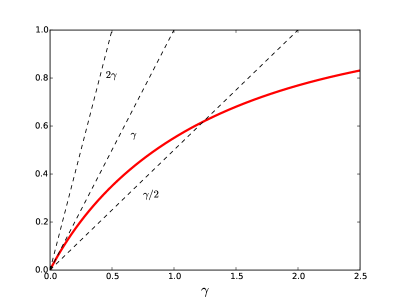
Figure 1: Illustration of the fixed point equation Eq. (8). The ‘effective signal-to-noise ratio’ $\gamma_{*}(\lambda)$ is given by the intersection of the curve $\gamma\mapsto G(\gamma)=1-{\sf mmse}(\gamma)$, and the line $\gamma/\lambda$.

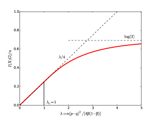
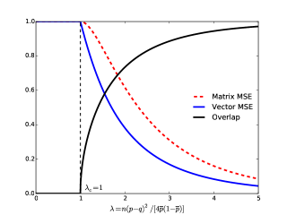
Figure 2: Left frame: Asymptotic mutual information per vertex of the two-groups stochastic block model, as a function of the signal-to-noise ratio $\lambda$. The dashed lines are simple upper bounds: $\lim_{n\to\infty}I({\boldsymbol{X}};{\boldsymbol{G}})/n\leq\lambda/4$ (cf. Lemma 3.1) and $I({\boldsymbol{X}};{\boldsymbol{G}})/n\leq\log 2$. Right frame: Asymptotic estimation error under different metrics (see Section 3.3). Note the phase transition at $\lambda=1$ in both frames.

Our asymptotic expression for the mutual information, cf. Theorem 1.1, and for the estimation error, cf. Theorem 1.4, depends on the solution of Eq. (8) which we copy here for the reader’s convenience:

$$\gamma =\lambda\big{(}1-{\sf mmse}(\gamma)\big{)}\;\equiv\lambda\,G(\gamma)\,.$$ (28)

Here we defined

$$G(\gamma)=1-{\sf mmse}(\gamma)={\mathbb{E}}\big{\{}\tanh(\gamma+\sqrt{\gamma}\,Z)^{2}\big{\}}\,.$$ (29)

The effective signal-to-noise ratio $\gamma_{*}(\lambda)$ that enters Theorem 1.1 and Theorem 1.4 is the largest non-negative solution of Eq. (8). This equation is illustrated in Figure 1.

It is immediate to show from the definition (29) that $G(\,\cdot\,)$ is continuous on $[0,\infty)$ with $G(0)=0$, and $\lim_{\gamma\to\infty}G(\gamma)=1$. This in particular implies that $\gamma=0$ is always a solution of Eq. (8). Further, since ${\sf mmse}(\gamma)$ is monotone decreasing in the signal-to-noise ratio $\gamma$, $G(\gamma)$ is monotone increasing. As shown in the proof of Remark 6.1 (see Appendix B.2), $G(\,\cdot\,)$ is also strictly concave on $[0,\infty)$. This implies that Eq. (8) as at most one solution in $(0,\infty)$, and a strictly positive solution only exists if $\lambda G^{\prime}(0)=\lambda>1$.

We summarize these remarks below, and refer to Figure 2 for an illustration.

Lemma 3.2.

The effective SNR, and the asymptotic expression for the per-vertex mutual information in Theorem 1.1 have the following properties:

• For $\lambda\leq 1$, we have $\gamma_{*}(\lambda)=0$ and $\Psi(\gamma_{*}(\lambda),\lambda)=\lambda/4$.

• For $\lambda\leq 1$, we have $\gamma_{*}(\lambda)\in(0,\lambda)$ strictly with $\gamma_{*}(\lambda)/\lambda\to 1$ as $\lambda\to\infty$.

  Further, $\Psi(\gamma_{*}(\lambda),\lambda)<\lambda/4$ strictly with $\Psi(\gamma_{*}(\lambda),\lambda)\to\log 2$ as $\gamma\to\infty$.

Proof.

All of the claims follow immediately form the previous remarks, and simple calculus, except the claim $\Psi(\gamma_{*}(\lambda),\lambda)<\lambda/4$ for $\lambda>1$. This is direct consequence of the variational characterization established below. ∎

We next give an alternative (variational) characterization of the asymptotic formula which is useful for proving bounds.

Lemma 3.3.

Under the assumptions and definitions of Theorem 1.1, we have

$$\lim_{n\to\infty}\frac{1}{n}\,I({\boldsymbol{X}};{\boldsymbol{G}})=\Psi(\gamma_{*}(\lambda),\lambda)=\min_{\gamma\in[0,\infty)}\,\Psi(\gamma,\lambda)\,.$$ (30)

Proof.

The function $\gamma\mapsto\Psi(\gamma,\lambda)$ is differentiable on $[0,\infty)$ with $\Psi(\gamma,\lambda)=\gamma^{2}/(4\lambda)+O(\gamma)\to\infty$ as $\gamma\to\infty$. Hence, the $\min_{\gamma\in[0,\infty)}\,\Psi(\gamma,\lambda)$ is achieved at a point where the first derivative vanishes (or, eventually, at $0$). Using the I-MMSE relation [GSV05], we get

$$\frac{\partial\Psi}{\partial\gamma}(\gamma,\lambda)=\frac{\gamma}{2\lambda}-\frac{1}{2}+\frac{1}{2}\,{\sf mmse}(\gamma)\,.$$ (31)

Hence the minimizer is a solution of Eq. (8). As shown above, for $\lambda\leq 1$, the only solution is $\gamma_{*}(\lambda)=0$, which therefore yields $\Psi(\gamma_{*}(\lambda),\lambda)=\min_{\gamma\in[0,\infty)}\,\Psi(\gamma,\lambda)$ as claimed.

For $\lambda>1$, Eq. (8) admits the two solutions: $0$ and $\gamma_{*}(\lambda)>0$. However, by expanding Eq. (31) for small $\gamma$, we obtain $\Psi(\gamma,\lambda)=\Psi(0,\lambda)-(1-\lambda^{-1})\gamma^{2}/4+o(\gamma)$ and hence $\gamma=0$ is a local maximum, which implies the claim for $\lambda>1$ as well. ∎

We conclude by noting that Eq. (8) can be solved numerically rather efficiently. The simplest method consists is by iteration. Namely, we initialize $\gamma^{0}=\lambda$ and then iterate $\gamma^{t+1}=\lambda\,G(\gamma^{t})$. This approach was used for Figure 2.

3.3 Consequences for estimation

Theorem 1.4 establishes that a phase transition takes place at $\lambda=1$ for the matrix minimum mean square error ${\sf MMSE}_{n}(\lambda_{n})$ defined in Eq. (14). Throughout this section, we will omit the subscript $n$ to denote the $n\to\infty$ limit (for instance, we write ${\sf MMSE}(\lambda)\equiv\lim_{n\to\infty}{\sf MMSE}_{n}(\lambda_{n})$).

Figure 2 reports the asymptotic prediction for ${\sf MMSE}(\lambda)$ stated in Theorem 1.4, and evaluated as discussed above. The error decreases rapidly to $0$ for $\lambda>1$.

In this section we discuss two other estimation metrics. In both cases we define these metrics by optimizing a suitable risk over a class of estimators: it is understood that randomized estimators are admitted as well.

• The first metric is the vector minimum mean square error:

  $${\sf vmmse}_{n}(\lambda_{n}) =\frac{1}{n}\,\inf_{{\boldsymbol{\widehat{x}}}:\mathcal{G}_{n}\to\mathbb{R}^{n}}{\mathbb{E}}\Big{\{}\min_{s\in\{+1,-1\}}\big{\|}{\boldsymbol{X}}-s\,{\boldsymbol{\widehat{x}}}({\boldsymbol{G}})\big{\|}_{2}^{2}\Big{\}}\,.$$ (32)

  Note the minimization over the sign $s$: this is necessary because the vertex labels can be estimated only up to an overall flip. Of course ${\sf vmmse}_{n}(\lambda_{n})\in[0,1]$, since it is always possible to achieve vector mean square error equal to one by returning ${\boldsymbol{\widehat{x}}}({\boldsymbol{G}})=0$.

• The second metric is the overlap:

  $${\sf Overlap}_{n}(\lambda_{n})=\frac{1}{n}\sup_{{\boldsymbol{\widehat{s}}}:\mathcal{G}_{n}\to\{+1,-1\}^{n}}{\mathbb{E}}\big{\{}|\langle{\boldsymbol{X}},{\boldsymbol{\widehat{s}}}({\boldsymbol{G}})\rangle|\big{\}}\,.$$ (33)

  Again ${\sf Overlap}_{n}(\lambda_{n})\in[0,1]$ (but now large overlap corresponds to good estimation). Indeed by returning $\widehat{x}_{i}({\boldsymbol{G}})\in\{+1,-1\}$ uniformly at random, we obtain ${\mathbb{E}}\big{\{}|\langle{\boldsymbol{X}},{\boldsymbol{\widehat{s}}}({\boldsymbol{G}})\rangle|\big{\}}/n=O(n^{-1/2})\to 0$.

  Note that the main difference between overlap and vector minimum mean square error is that in the latter case we consider estimators ${\boldsymbol{\widehat{x}}}:\mathcal{G}_{n}\to\mathbb{R}^{n}$ taking arbitrary real values, while in the former we assume estimators ${\boldsymbol{\widehat{s}}}:\mathcal{G}_{n}\to\{+1,-1\}^{n}$ taking binary values.

In order to clarify the relation between various metrics, we begin by proving the alternative characterization of the matrix minimum mean square error in Eqs. (18), (19).

Lemma 3.4.

Letting ${\sf MMSE}_{n}(\lambda)$ be defined as per Eq. (14), we have

$${\sf MMSE}_{n}(\lambda) ={\mathbb{E}}\big{\{}\big{[}X_{2}-{\mathbb{E}}\{X_{2}|X_{1}=+1,{\boldsymbol{G}}\}\big{]}^{2}\big{|}X_{1}=+1\big{\}}$$ (34)

$$=\min_{\widehat{x}_{2|1}:\mathcal{G}_{n}\to\mathbb{R}}{\mathbb{E}}\big{\{}\big{[}X_{2}-\widehat{x}_{2|1}({\boldsymbol{G}})\big{]}^{2}|X_{1}=+1\big{\}}\,.$$ (35)

Proof.

First note that Eq. (35) follows immediately from Eq. (34) since conditional expectation minimizes the mean square error (the conditioning only changes the prior on ${\boldsymbol{X}}$).

In order to prove Eq. (34), we start from Eq. (16). Since the prior distribution on $X_{1}$ is uniform, we have

$${\mathbb{E}}\{X_{1}X_{2}|{\boldsymbol{G}}\} =\frac{1}{2}{\mathbb{E}}\{X_{1}X_{2}|X_{1}=+1,{\boldsymbol{G}}\}+\frac{1}{2}{\mathbb{E}}\{X_{1}X_{2}|X_{1}=+1,{\boldsymbol{G}}\}$$ (36)

$$={\mathbb{E}}\{X_{2}|X_{1}=+1,{\boldsymbol{G}}\}\,.$$ (37)

where in the second line we used the fact that, conditional to ${\boldsymbol{G}}$, ${\boldsymbol{X}}$ is distributed as $-{\boldsymbol{X}}$. Continuing from Eq. (16), we get

$${\sf MMSE}_{n}(\lambda) ={\mathbb{E}}\big{\{}\big{[}X_{1}X_{2}-{\mathbb{E}}\{X_{2}|X_{1}=+1,{\boldsymbol{G}}\}\big{]}^{2}\big{\}}$$ (38)

$$=\frac{1}{2}\,{\mathbb{E}}\big{\{}\big{[}X_{1}X_{2}-{\mathbb{E}}\{X_{2}|X_{1}=+1,{\boldsymbol{G}}\}\big{]}^{2}\big{|}X_{1}=+1\big{\}}$$

$$\phantom{aaaa}+\frac{1}{2}\,{\mathbb{E}}\big{\{}\big{[}X_{1}X_{2}-{\mathbb{E}}\{X_{2}|X_{1}=+1,{\boldsymbol{G}}\}\big{]}^{2}\big{|}X_{1}=-1\big{\}}$$ (39)

$$={\mathbb{E}}\big{\{}\big{[}X_{2}-{\mathbb{E}}\{X_{2}|X_{1}=+1,{\boldsymbol{G}}\}\big{]}^{2}\big{|}X_{1}=+1\big{\}}\,,$$ (40)

which proves the claim. ∎

The next lemma clarifies the relationship between matrix and vector minimum mean square error. Its proof is deferred to Appendix A.1.

Lemma 3.5.

With the above definitions, we have

$$1-\sqrt{1-(1-n^{-1}){\sf MMSE}_{n}(\lambda)}\leq{\sf vmmse}_{n}(\lambda)\leq{\sf MMSE}_{n}(\lambda)\,.$$ (41)

Finally, a lemma that relates overlap and vector minimum mean square error, whose proof can be found in Appendix A.2.

Lemma 3.6.

With the above definitions, we have

$${\sf Overlap}_{n}(\lambda)\geq 1-{\sf vmmse}_{n}(\lambda)-O(n^{-1/2})\,.$$ (42)

As an immediate corollary of these lemmas (together with Theorem 1.4 and Lemma 3.2), we obtain that $\lambda=1$ is the critical point for other estimation metrics as well.

Corollary 3.7.

The vector minimum mean square error and the overlap exhibit a phase transition at $\lambda=1$. Namely, under the assumptions of Theorem 1.1 (in particular, $\lambda_{n}\to\lambda$ and $n\overline{p}_{n}(1-\overline{p}_{n})\to\infty$), we have

• If $\lambda\leq 1$, then estimation cannot be performed asymptotically better than without any information:

  $$\lim_{n\to\infty}{\sf vmmse}_{n}(\lambda_{n}) =1\,,$$ (43)

  $$\lim_{n\to\infty}{\sf Overlap}_{n}(\lambda_{n}) =0\,.$$ (44)

• If $\lambda>1$, then estimation can be performed better than without any information, even in the limit $n\to\infty$:

  $$0<1-\frac{\gamma_{*}(\lambda)}{\lambda}\leq\liminf_{n\to\infty}{\sf vmmse}_{n}(\lambda_{n})\leq\limsup_{n\to\infty}{\sf vmmse}_{n}(\lambda_{n})\leq 1-\frac{\gamma_{*}(\lambda)^{2}}{\lambda^{2}}<1\,,$$ (45)

  $$0<\frac{\gamma_{*}(\lambda)^{2}}{\lambda^{2}}\leq\liminf_{n\to\infty}{\sf Overlap}_{n}(\lambda_{n})\,.$$ (46)

4 Proof strategy: Theorem 1.1

In this section we describe the main elements used in the proof of Theorem 1.1:

• We describe a Gaussian observation model which has asymptotically the same mutual information as the SBM introduced above.

• We state an asymptotic characterization of the mutual information of this Gaussian model.

• We describe an approximate message passing (AMP) estimation algorithm that plays a key role in the last characterization.

We then use these technical results (proved in later sections) to prove Theorem 1.1 in Section 4.3.

We recall that $\overline{p}_{n}=(p_{n}+q_{n})/2$. Define the gap $\Delta_{n}\equiv(p_{n}-q_{n})/2=\sqrt{\lambda_{n}\overline{p}_{n}(1-\overline{p}_{n})/n}$. We will assume for the proofs that $\lim_{n\to\infty}\lambda_{n}=\lambda>0$ (i.e. the assortative model) but the results also hold for $\lambda<0$ in an analogous fashion.

4.1 Gaussian model

The edges $\{G_{ij}\}_{i<j}$ are conditionally independent given the vertex labels ${\boldsymbol{X}}$, with distribution:

$$G_{ij} =\begin{cases}1&\text{ with probability }\overline{p}_{n}+\Delta_{n}X_{i}X_{j}\,,\\ 0&\text{ with probability }1-\overline{p}_{n}-\Delta_{n}X_{i}X_{j}\,.\end{cases}$$ (47)

As a first step, we compare the SBM with an alternate Gaussian observation model defined as follows. Let ${\boldsymbol{Z}}$ be a Gaussian random symmetric matrix generated with independent entries $Z_{ij}\sim{\sf N}(0,1)$ and $Z_{ii}\sim{\sf N}(0,2)$, independent of ${\boldsymbol{X}}$. Consider the noisy observations ${\boldsymbol{Y}}={\boldsymbol{Y}}(\lambda)$ defined by

$${\boldsymbol{Y}}(\lambda) =\sqrt{\frac{\lambda}{n}}{\boldsymbol{X}}{\boldsymbol{X}}^{\sf T}+{\boldsymbol{Z}}\,.$$ (48)

Note that this model matches the first two moments of the original model. More precisely, if we define the rescaled adjacency matrix $G^{\rm res}_{ij}\equiv(G_{ij}-\overline{p}_{n})/\sqrt{\overline{p}_{n}(1-\overline{p}_{n})}$, then ${\mathbb{E}}\{G^{\rm res}_{ij}|{\boldsymbol{X}}\}={\mathbb{E}}\{Y_{ij}|{\boldsymbol{X}}\}$ and ${\rm Var}(G^{\rm res}_{ij}|{\boldsymbol{X}})={\rm Var}(Y_{ij}|{\boldsymbol{X}})+O(n^{-1/2})$.

Our first proposition proves that the mutual information between the vertex labels ${\boldsymbol{X}}$ and the observations agrees to leading order across the two models.

Proposition 4.1.

Assume that, as $n\to\infty$, $(i)$ $\lambda_{n}\to\lambda$ and $(ii)$ $n\overline{p}_{n}(1-\overline{p}_{n})\to\infty$. Then there is a constant $C$ independent of $n$ such that

$$\frac{1}{n}\big{|}I({\boldsymbol{X}};{\boldsymbol{G}})-I({\boldsymbol{X}};{\boldsymbol{Y}})\big{|}\leq C\left(\frac{\lambda^{3/2}}{\sqrt{n\overline{p}_{n}(1-\overline{p}_{n})}}+\left\lvert{\lambda_{n}-\lambda}\right\rvert\right).$$ (49)

The proof of this result is presented in Section 5.

The next step consists in analyzing the Gaussian model (48), which is of independent interest. It turns out to be convenient to embed this in a more general model whereby, in addition to the observations ${\boldsymbol{Y}}$, we are also given observations of ${\boldsymbol{X}}$ through a binary erasure channel with erasure probability ${\boldsymbol{{\varepsilon}}}=1-{\varepsilon}$, ${\sf BEC}({\boldsymbol{{\varepsilon}}})$. We will denote by ${\boldsymbol{X}}({\varepsilon})=(X_{1}({\varepsilon}),\dots,X_{n}({\varepsilon}))$ the output of this channel, where we set $X_{i}({\varepsilon})=0$ every time the symbol is erased. Formally we have

$$X_{i}({\varepsilon})=B_{i}\,X_{i}\,,$$ (50)

where $B_{i}\sim{\sf Ber}({\varepsilon})$ are independent random variables, independent of ${\boldsymbol{X}}$, ${\boldsymbol{G}}$. In the special case ${\varepsilon}=0$, all of these observations are trivial, and we recover the original model.

The reason for introducing the additional observations ${\boldsymbol{X}}({\varepsilon})$ is the following. The graph ${\boldsymbol{G}}$ has the same distribution conditional on ${\boldsymbol{X}}$ or $-{\boldsymbol{X}}$, hence it is impossible to recover the sign of ${\boldsymbol{X}}$. As we will see, the extra observations ${\boldsymbol{X}}({\varepsilon})$ allow to break this trivial symmetry and we will recover the required results by continuity in ${\varepsilon}$ as the extra information vanishes.

Indeed, our next result establishes a single letter characterization of $I({\boldsymbol{X}};{\boldsymbol{Y}},{\boldsymbol{X}}({\varepsilon}))$ in terms of a recalibrated scalar observation problem. Namely, we define the following observation model for $X_{0}\sim{\rm Uniform}(\{+1,-1\})$ a Rademacher random variable:

$$Y_{0} =\sqrt{\gamma}X_{0}+Z_{0},$$ (51)

$$X_{0}({\varepsilon}) =B_{0}X_{0}\,.$$ (52)

Here $X_{0}$, $B_{0}\sim{\sf Ber}({\varepsilon})$, $Z_{0}\sim{\sf N}(0,1)$, are mutually independent. We denote by ${\sf mmse}(\gamma,{\varepsilon})$, the minimum mean squared error of estimating $X_{0}$ from $X_{0}({\varepsilon})$, $Y_{0}$, conditional on $B_{0}$. Recall the definitions (4), (5) of ${\sf I}(\gamma)$, ${\sf mmse}(\gamma)$, and the expressions (6), (7). A simple calculation yields

$${\sf mmse}(\gamma,{\varepsilon}) ={\mathbb{E}}\left\{(X_{0}-{\mathbb{E}}\left\{X_{0}|X_{0}({\varepsilon}),Y_{0}\right\})^{2}\right\}$$ (53)

$$=(1-{\varepsilon})\,{\sf mmse}(\gamma)\,.$$ (54)

Proposition 4.2.

For any $\lambda>0$, ${\varepsilon}\in(0,1]$, let $\gamma_{*}(\lambda,{\varepsilon})$ be the largest non-negative solution of the equation:

$$\gamma =\lambda\,\big{(}1-(1-{\varepsilon}){\sf mmse}(\gamma)\big{)}\,.$$ (55)

Further, define $\Psi(\gamma,\lambda,{\varepsilon})$ by:

$$\Psi(\gamma,\lambda,{\varepsilon}) =\frac{\lambda}{4}+\frac{\gamma^{2}}{4\lambda}-\frac{\gamma}{2}+{\varepsilon}\,\log 2+(1-{\varepsilon})\,{\sf I}(\gamma)\,.$$ (56)

Then, we have

$$\lim_{n\to\infty}\frac{1}{n}I({\boldsymbol{X}};{\boldsymbol{X}}({\varepsilon}),{\boldsymbol{Y}}) =\Psi\big{(}\gamma_{*}(\lambda,{\varepsilon}),\lambda,{\varepsilon}\big{)}\,.$$ (57)

Using continuity in ${\varepsilon}$, the last result implies directly a limit result for the mutual information under the Gaussian model, which we single out since it is of independent interest.

Theorem 4.3.

For any $\lambda>0$, let $\gamma_{*}(\lambda)$ be the largest non-negative solution of the equation:

$$\gamma =\lambda\,\big{(}1-{\sf mmse}(\gamma)\big{)}\,.$$ (58)

Further, define $\Psi(\gamma,\lambda)$ by:

$$\Psi(\gamma,\lambda) =\frac{\lambda}{4}+\frac{\gamma^{2}}{4\lambda}-\frac{\gamma}{2}+{\sf I}(\gamma)\,.$$ (59)

Then, we have

$$\lim_{n\to\infty}\frac{1}{n}I({\boldsymbol{X}};{\boldsymbol{Y}}) =\Psi\big{(}\gamma_{*}(\lambda),\lambda\big{)}\,.$$ (60)

4.2 Approximate Message Passing (AMP)

To analyze the Gaussian model Eq. (48) we introduce an approximate message passing (AMP) algorithm that computes estimates ${\boldsymbol{x}}^{t}\in\mathbb{R}^{n}$ at time $t$, which are functions of the observations ${\boldsymbol{Y}},{\boldsymbol{X}}({\varepsilon})$. This construction follows the general scheme of AMP algorithms developed in [DMM09, BM11, JM13]. Given a sequence of functions $f_{t}:\mathbb{R}\times\left\{-1,0,+1\right\}\to\mathbb{R}$, we set ${\boldsymbol{x}}^{0}=0$ and compute

$${\boldsymbol{x}}^{t+1} =\frac{{\boldsymbol{Y}}(\lambda)}{\sqrt{n}}f_{t}({\boldsymbol{x}}^{t},{\boldsymbol{X}}({\varepsilon}))-{\sf b}_{t}f_{t-1}({\boldsymbol{x}}^{t-1},{\boldsymbol{X}}({\varepsilon}))\,,$$ (61)

$${\sf b}_{t} =\frac{1}{n}\sum_{i=1}^{n}f_{t}^{\prime}({\boldsymbol{x}}^{t}_{i},{\boldsymbol{X}}({\varepsilon})_{i})\,.$$ (62)

Above (and in the sequel) we extend the function $f_{t}$ to vectors by applying it component-wise, i.e. $f_{t}({\boldsymbol{x}}^{t},{\boldsymbol{X}}({\varepsilon}))=(f_{t}(x^{t}_{1},X({\varepsilon})_{1}),f_{t}(x^{t}_{2},X({\varepsilon})_{2}),\dots f_{t}(x^{t}_{n},X({\varepsilon})_{n}))$.

The AMP iteration above proceeds analogously to the usual power iteration to compute principal eigenvectors, but has an additional memory term $-{\sf b}_{t}f_{t-1}({\boldsymbol{x}}^{t-1})$. This additional term changes the behavior of the iterates in an important way: unlike the usual power iteration, there is an explicit distributional characterization of the iterates ${\boldsymbol{x}}^{t}$ in the limit of large dimension. Namely, for each time $t$ we will show that, approximately $x^{t}_{i}$ is a scaled version of the truth $X_{i}$ observed through Gaussian noise of a certain variance. We define the following two-parameters recursion, with initialization $\mu_{0}=\sigma_{0}=0$, which will be referred to as state evolution:

$$\mu_{t+1} =\sqrt{\lambda}\,{\mathbb{E}}\left\{X_{0}f_{t}(\mu_{t}X_{0}+\sigma_{t}Z_{0},X_{0}({\varepsilon}))\right\}\,,$$ (63)

$$\sigma^{2}_{t+1} ={\mathbb{E}}\left\{f_{t}(\mu_{t}X_{0}+\sigma_{t}Z_{0},X_{0}({\varepsilon}))^{2}\right\}\,,$$ (64)

where expectation is with respect to the independent random variables $X_{0}\sim{\rm Uniform}(\{+1,-1\})$, $Z_{0}\sim{\sf N}(0,1)$ and $B_{0}\sim{\sf Ber}(1-{\varepsilon})$, setting $X_{0}({\varepsilon})=B_{0}X_{0}$.

The following lemma makes this distributional characterization precise. It follows from the more general result of [JM13] and we provide a proof in Appendix B.

Lemma 4.4 (State Evolution).

Let $f_{t}:\mathbb{R}\times\{-1,0,1\}\to\mathbb{R}$ be a sequence of functions such that $f_{t},f^{\prime}_{t}$ are Lipschitz continuous in their first argument (where $f^{\prime}_{t}$ denotes the derivative of $f_{t}$ with respect to the first argument).

Let $\psi:\mathbb{R}\times\{+,1-1\}\times\{+1,0,-1\}\to\mathbb{R}$ be a test function such that $|\psi(x_{1},s,r)-\psi(x_{2},s,r)|\leq C(1+|x_{1}|+|x_{2}|)\,|x_{1}-x_{2}|$ for all $x_{1},x_{2},s,r$. Then the following limit holds almost surely for $(X_{0},Z_{0},X_{0}({\varepsilon}))$ random variables distributed as above

$$\lim_{n\to\infty}\frac{1}{n}\sum_{i=1}^{n}\psi(x^{t}_{i},X_{i},X({\varepsilon})_{i}) ={\mathbb{E}}\left\{\psi\big{(}\mu_{t}X_{0}+\sigma_{t}Z_{0},X_{0},X_{0}({\varepsilon})\big{)}\right\}\,,$$ (65)

Although the above holds for a relatively broad class of functions $f_{t}$, we are interested in the AMP algorithm for specific functions $f_{t}$. Specifically, we following sequence of functions

$$f_{t}(y,s) ={\mathbb{E}}\big{\{}X_{0}|\mu_{t}X_{0}+\sigma_{t}Z_{0}=y,\,X_{0}({\varepsilon})=s\big{\}}\,.$$ (66)

It is easy to see that $f_{t}$ satisfy the requirement of Lemma 4.4. We will refer to this version of AMP as Bayes-optimal AMP.

Note that the definition (66) depends itself on $\mu_{t}$ and $\sigma_{t}$ defined through Eqs. (63), (63). This recursive definition is perfectly well defined and yields

$$\mu_{t+1} =\sqrt{\lambda}{\mathbb{E}}\big{\{}X_{0}{\mathbb{E}}\{X_{0}|\mu_{t}X_{0}+\sigma_{t}Z_{0},X({\varepsilon})_{0}\}\big{\}},$$ (67)

$$\sigma_{t+1}^{2} ={\mathbb{E}}\big{\{}{\mathbb{E}}\{X_{0}|\mu_{t}X_{0}+\sigma_{t}Z_{0},X({\varepsilon})_{0}\}^{2}\big{\}}\,.$$ (68)

Using the fact that $f_{t}(y,s)={\mathbb{E}}\{X_{0}|\mu_{t}X_{0}+\sigma_{t}Z_{0}=y,\,X_{0}({\varepsilon})=s\}$ is the minimum mean square error estimator, we obtain

$$\mu_{t+1} =\sqrt{\lambda}\sigma_{t+1}^{2}\,,$$ (69)

$$\sigma_{t+1}^{2} =1-(1-{\varepsilon})\,{\sf mmse}(\lambda\sigma_{t}^{2})\,,$$ (70)

where ${\sf mmse}(\,\cdot\,)$ is given explicitly by Eq. (7).

In other words, the state evolution recursion reduces to a simple one-dimensional recursion that we can write in terms of the variable $\gamma_{t}\equiv\lambda\sigma_{t}^{2}$. We obtain

$$\gamma_{t+1} =\lambda\big{(}1-(1-{\varepsilon})\,{\sf mmse}(\gamma_{t})\big{)}\,,$$ (71)

$$\sigma^{2}_{t}=\frac{\gamma_{t}}{\lambda}\,,\;\;\;\;\mu_{t}=\frac{\gamma_{t}}{\sqrt{\lambda}}$$ (72)

Our proof strategy uses the AMP algorithm to construct estimates that bound from above the minimum error of estimating ${\boldsymbol{X}}$ from observations ${\boldsymbol{Y}},{\boldsymbol{X}}({\varepsilon})$. However, in the limit of a large number of iterations, we show that the gap between this upper bound and the minimum estimation error vanishes via an area theorem.

More explicitly, we develop an upper bound on the matrix mean square error first introduced in Eq. (14). We generalize this in the obvious way to the Gaussian observation model:

$${\sf MMSE}(\lambda,{\varepsilon},n) \equiv\frac{1}{n^{2}}\,{\mathbb{E}}\Big{\{}\big{\|}{\boldsymbol{X}}{\boldsymbol{X}}^{{\sf T}}-{\mathbb{E}}\{{\boldsymbol{X}}{\boldsymbol{X}}^{{\sf T}}|{\boldsymbol{X}}({\varepsilon}),{\boldsymbol{Y}}\}\big{\|}_{F}^{2}\Big{\}}\,.$$ (73)

(Note that we adopt here a slightly different normalization with respect to Eq. (14). This change is immaterial in the large $n$ limit.)

We then use AMP to construct the sequence of estimators ${\boldsymbol{\widehat{x}}}^{t}=f_{t-1}({\boldsymbol{x}}^{t-1},{\boldsymbol{X}}({\varepsilon}))$, indexed by $t\in\{1,2,\dots\}$, where $f_{t-1}$ is defined as in Eq. (66). The matrix mean squared error of this estimators will be denoted by

$${\sf MSE}_{\sf AMP}(t;\lambda,{\varepsilon},n) \equiv\frac{1}{n^{2}}\,{\mathbb{E}}\Big{\{}\big{\|}{\boldsymbol{X}}{\boldsymbol{X}}^{\sf T}-{\boldsymbol{\widehat{x}}}^{t}({\boldsymbol{\widehat{x}}}^{t})^{\sf T}\big{\|}^{2}\Big{\}}\,.$$ (74)

We also define the limits

$${\sf MSE}_{\sf AMP}(t;\lambda,{\varepsilon}) \equiv\lim_{n\to\infty}{\sf MSE}_{\sf AMP}(t;\lambda,{\varepsilon})\,,$$ (75)

$${\sf MSE}_{\sf AMP}(\lambda,{\varepsilon}) =\lim_{t\to\infty}{\sf mse_{\sf AMP}}(t;\lambda,{\varepsilon})\,.$$ (76)

In the course of the proof, we will also see that these limits are well-defined, using the state evolution Lemma 4.4

4.3 Proof of Theorem 1.1 and Theorem 4.3

The proof is almost immediate given Propositions 4.1 and 4.2. Firstly, note that, for any ${\varepsilon}\in(0,1]$,

$$\left|\frac{1}{n}I({\boldsymbol{X}};{\boldsymbol{X}}({\varepsilon}),{\boldsymbol{Y}})-\frac{1}{n}I({\boldsymbol{X}};{\boldsymbol{Y}})\right|\leq\frac{1}{n}I({\boldsymbol{X}};{\boldsymbol{X}}({\varepsilon}),{\boldsymbol{Y}})\leq{\varepsilon}\log 2$$ (77)

Since, by Proposition 4.2 $I({\boldsymbol{X}};{\boldsymbol{X}}({\varepsilon}),{\boldsymbol{Y}})/n$ has a well-defined limit as $n\to\infty$, and ${\varepsilon}>0$ is arbitrary, we have that:

$$\lim_{n\to\infty}\frac{1}{n}I({\boldsymbol{X}};{\boldsymbol{Y}}) =\lim_{{\varepsilon}\to 0}\Psi(\gamma_{*}(\lambda,{\varepsilon}),\lambda,{\varepsilon})\,.$$ (78)

It is immediate to check that $\Psi(\gamma,\lambda,{\varepsilon})$ is continuous in ${\varepsilon}\geq 0$, $\gamma\geq 0$ and $\Psi(\gamma,\lambda,0)=\Psi(\gamma,\lambda)$ as defined in Theorem 1.1. Furthermore, as ${\varepsilon}\to 0$, the unique positive solution $\gamma_{*}(\lambda,{\varepsilon})$ of Eq. (55) converges to $\gamma_{*}(\lambda)$, the largest non-negative solution to of Eq. (8), which we copy here for the readers’ convenience:

$$\gamma =\lambda(1-{\sf mmse}(\gamma)).$$ (79)

This follows from the smoothness and concavity of the function $1-{\sf mmse}(\gamma)$ (see Lemma 6.1). It follows that $\lim_{{\varepsilon}\to 0}\Psi(\gamma_{*}(\lambda,{\varepsilon}),\lambda,{\varepsilon})=\Psi(\gamma_{*}(\lambda),\lambda)$ and therefore

$$\lim_{n\to\infty}\frac{1}{n}I({\boldsymbol{X}};{\boldsymbol{Y}}) =\Psi(\gamma_{*}(\lambda),\lambda),$$ (80)

This proves Theorem 4.3. Theorem 1.1 follows by applying Proposition 4.1.

5 Proof of Proposition 4.1

Given a collection ${\boldsymbol{V}}=(V_{ij})_{i<j}$ of random variables defined on the same probability space as ${\boldsymbol{X}}$, and a non-negative real number $\lambda$, we define the following Hamiltonian and log-partition function associated with it:

$${\cal H}({\boldsymbol{x}},{\boldsymbol{X}},{\boldsymbol{V}},\lambda,n) \equiv\sum_{i<j}V_{ij}(x_{i}x_{j}-X_{i}X_{j})+\frac{\lambda}{n}x_{i}x_{j}X_{i}X_{j}\,,$$ (81)

$$\phi(X,V,\lambda,n) \equiv\log\Big{\{}\sum_{x\in{\{\pm 1\}^{n}}}\exp\big{(}{\cal H}({\boldsymbol{x}},{\boldsymbol{X}},{\boldsymbol{V}},\lambda,n)\big{)}\Big{\}}\,.$$ (82)

Lemma 5.1.

We have the identity:

$$I({\boldsymbol{X}};{\boldsymbol{Y}})=n\log 2+\frac{(n-1)\lambda}{2}-{\mathbb{E}}_{X,Z}\left\{\phi({\boldsymbol{X}},{\boldsymbol{Z}}\sqrt{\lambda/n},\lambda,n)\right\}\,.$$ (83)

Proof.

By definition:

$$I({\boldsymbol{X}};{\boldsymbol{Y}}) ={\mathbb{E}}\left\{\log\frac{{\mathrm{d}}p_{{\boldsymbol{Y}}|{\boldsymbol{X}}}({\boldsymbol{Y}}|{\boldsymbol{X}})}{{\mathrm{d}}p_{\boldsymbol{Y}}({\boldsymbol{Y}}(\lambda))}\right\}.$$ (84)

Since the two distributions $p_{{\boldsymbol{Y}}|{\boldsymbol{X}}}$ and $p_{{\boldsymbol{Y}}}$ are absolutely continuous with respect to each other, we can write the above simply in terms of the ratio of (Lebesgue) densities, and we obtain:

$$I(X;Y) ={\mathbb{E}}\log\left\{\frac{\exp\big{(}-\big{\|}{\boldsymbol{Y}}-\sqrt{\lambda/n}{\boldsymbol{X}}{\boldsymbol{X}}^{\sf T}\big{\|}_{F}^{2}/4\big{)}}{\sum_{x\in{\{\pm 1\}^{n}}}2^{-n}\exp\big{(}-\big{\|}{\boldsymbol{Y}}-\sqrt{\lambda/n}{\boldsymbol{x}}{\boldsymbol{x}}^{\sf T}\big{\|}_{F}^{2}/4\big{)}}\right\}$$ (85)

$$=n\log 2-{\mathbb{E}}_{{\boldsymbol{X}},{\boldsymbol{Z}}}\log\left\{\sum_{x\in{\{\pm 1\}^{n}}}\exp\left(-\frac{1}{2}\sum_{i<j}\Big{(}Z_{ij}+\sqrt{\frac{\lambda}{n}}(X_{i}X_{j}-x_{i}x_{j})\Big{)}^{2}+\frac{1}{2}Z_{ij}^{2})\right)\right\}$$ (86)

$$=n\log 2-{\mathbb{E}}_{{\boldsymbol{X}},{\boldsymbol{Z}}}\log\left\{\sum_{x\in{\{\pm 1\}^{n}}}\exp\left(\sum_{i<j}\sqrt{\frac{\lambda}{n}}Z_{ij}(x_{i}x_{j}-X_{i}X_{j})-\frac{\lambda}{2n}(x_{i}x_{j}-X_{i}X_{j})^{2}\right)\right\}\,.$$ (87)

We modify the final term as follows:

$$\sum_{i<j}(x_{i}x_{j}-X_{i}X_{j})^{2} =\sum_{i<j}2-2x_{i}x_{j}X_{i}X_{j}$$ (88)

$$=n(n-1)-2\sum_{i<j}x_{i}x_{j}X_{i}X_{j}.$$ (89)

Substituting this in Eq. (87) we have

$$I({\boldsymbol{X}};{\boldsymbol{Y}}) =n\log 2-{\mathbb{E}}_{{\boldsymbol{X}},{\boldsymbol{Z}}}\log\left\{\sum_{x\in{\{\pm 1\}^{n}}}\exp\Big{(}\sum_{i<j}\sqrt{\frac{\lambda}{n}}Z_{ij}(x_{i}x_{j}-X_{i}X_{j})+\frac{\lambda}{n}x_{i}x_{j}X_{i}X_{j}\Big{)}\right\}+\frac{1}{2}\lambda(n-1),$$ (90)

as required. ∎

Lemma 5.2.

Define the (random) Hamiltonian ${\cal{H}_{\mathrm{SBM}}}(x,\lambda,n)$ by:

$${\cal{H}_{\mathrm{SBM}}}({\boldsymbol{x}},{\boldsymbol{X}},{\boldsymbol{G}},n) \equiv\sum_{i<j}\left\{G_{ij}\log\left(\frac{\overline{p}_{n}+\Delta_{n}x_{i}x_{j}}{\overline{p}_{n}+\Delta_{n}X_{i}X_{j}}\right)+(1-G_{ij})\log\left(\frac{1-\overline{p}_{n}-\Delta_{n}x_{i}x_{j}}{1-\overline{p}_{n}-\Delta_{n}X_{i}X_{j}}\right)\right\}\,.$$ (91)

Then we have that:

$$I({\boldsymbol{X}};{\boldsymbol{G}}) =n\log 2-{\mathbb{E}}_{{\boldsymbol{X}},{\boldsymbol{G}}}\log\left\{\sum_{{\boldsymbol{x}}\in{\{\pm 1\}^{n}}}\exp({\cal{H}_{\mathrm{SBM}}}({\boldsymbol{x}},{\boldsymbol{X}},{\boldsymbol{G}},n))\right\}\,.$$ (92)

Proof.

This follows directly from the definition of mutual information:

$$I({\boldsymbol{X}};{\boldsymbol{G}}) ={\mathbb{E}}_{{\boldsymbol{X}},{\boldsymbol{G}}}\left\{\frac{{\mathrm{d}}p_{{\boldsymbol{G}}|{\boldsymbol{X}}}({\boldsymbol{G}}|{\boldsymbol{X}})}{{\mathrm{d}}p_{{\boldsymbol{G}}}({\boldsymbol{G}})}\right\}\,.$$ (93)

As in Lemma 5.1 we can write this in terms of densities as:

$$\frac{{\mathrm{d}}p_{{\boldsymbol{G}}|{\boldsymbol{X}}}({\boldsymbol{G}}|{\boldsymbol{X}})}{{\mathrm{d}}p_{\boldsymbol{G}}({\boldsymbol{G}})} =\frac{\prod_{i<j}(\overline{p}_{n}+\Delta_{n}X_{i}X_{j})^{G_{ij}}(1-\overline{p}_{n}-\Delta_{n}X_{i}X_{j})^{1-G_{ij}}}{\sum_{x\in{\{\pm 1\}^{n}}}2^{-n}\prod_{i<j}(\overline{p}_{n}+\Delta_{n}x_{i}x_{j})^{G_{ij}}(\overline{p}_{n}+\Delta_{n}X_{i}X_{j})^{1-G_{ij}}}$$ (94)

Substituting this in the mutual information formula Eq. (93) yields the lemma. ∎

Define the random variables $\boldsymbol{\widetilde{G}}=(\widetilde{G}_{ij})_{i<j}$ as follows:

$$\widetilde{G}_{ij} \equiv\frac{\Delta_{n}}{\overline{p}_{n}(1-\overline{p}_{n})}(G_{ij}-\overline{p}_{n}-\Delta_{n}X_{i}X_{j}).$$ (95)

The following lemma shows that, to compute $I({\boldsymbol{X}};{\boldsymbol{G}})$ it suffices to compute the log-partition function with respect to the approximating Hamiltonian.

Lemma 5.3.

Assume that, as $n\to\infty$, $(i)$ $\lambda_{n}\to\lambda$ and $(ii)$ $n\overline{p}_{n}(1-\overline{p}_{n})\to\infty$. Then, we have

$$I({\boldsymbol{X}};{\boldsymbol{G}}) =n\log 2+\frac{(n-1)\lambda_{n}}{2}-{\mathbb{E}}_{{\boldsymbol{X}},\boldsymbol{\widetilde{G}}}\left\{\phi({\boldsymbol{X}},\boldsymbol{\widetilde{G}},\lambda_{n},n)\right\}+O\left(\frac{n\lambda^{3/2}}{\sqrt{n\overline{p}_{n}(1-\overline{p}_{n})}}\right)\,.$$ (96)

Proof.

We concentrate on the log-partition function for the hamiltonian ${\cal{H}_{\mathrm{SBM}}}({\boldsymbol{x}},{\boldsymbol{X}},{\boldsymbol{G}},n)$. First, using the fact that $\log(c+dx)=\frac{1}{2}\log((c+d)(c-d))+\frac{x}{2}\log((c+d)/(c-d))$ when $x\in\{\pm 1\}$:

$${\cal{H}_{\mathrm{SBM}}}({\boldsymbol{x}},{\boldsymbol{X}},{\boldsymbol{G}},n) =(x_{i}x_{j}-X_{i}X_{j})\left(\frac{G_{ij}}{2}\log\left(\frac{1+\Delta_{n}/\overline{p}_{n}}{1-\Delta_{n}/\overline{p}_{n}}\right)+\frac{(1-G_{ij})}{2}\log\left(\frac{1-\Delta_{n}/(1-\overline{p}_{n})}{1+\Delta_{n}/(1-\overline{p}_{n})}\right)\right).$$ (97)

Now when $\max(\Delta_{n}/\overline{p}_{n},\Delta_{n}/(1-\overline{p}_{n}))\leq c_{0}$, for small enough $c_{0}$, we have by Taylor expansion the following approximation for $z\in[0,c_{0}]$:

$$\left\lvert{\frac{1}{2}\log\left(\frac{1+z}{1-z}\right)-z}\right\rvert \leq z^{3},$$ (98)

which implies, by triangle inequality:

$${\cal{H}_{\mathrm{SBM}}}({\boldsymbol{x}},{\boldsymbol{X}},{\boldsymbol{G}},n) =\sum_{i<j}(x_{i}x_{j}-X_{i}X_{j})\left(\frac{\Delta_{n}G_{ij}}{\overline{p}_{n}}-\frac{\Delta_{n}(1-G_{ij})}{1-\overline{p}_{n}}\right)+\text{err}_{n}\,,$$ (99)

where

$$\left\lvert{\text{err}_{n}}\right\rvert \leq C\Delta_{n}^{3}\left(\frac{\left\lvert{\langle{\boldsymbol{x}},{\boldsymbol{G}}{\boldsymbol{x}}\rangle}\right\rvert+\left\lvert{\langle{\boldsymbol{X}},{\boldsymbol{G}}{\boldsymbol{X}}\rangle}\right\rvert}{\overline{p}_{n}^{3}}+\frac{\left\lvert{\langle{\boldsymbol{x}},({\bf 1}{\bf 1}^{\sf T}-{\boldsymbol{G}}){\boldsymbol{x}}\rangle}\right\rvert+\left\lvert{\langle{\boldsymbol{X}},({\bf 1}{\bf 1}^{\sf T}-{\boldsymbol{G}}){\boldsymbol{X}}\rangle}\right\rvert}{(1-\overline{p}_{n})^{3}}\right).$$ (100)

We first simplify the RHS in Eq. (99). Recalling the definition of $\widetilde{G}_{ij}$:

$$\sum_{i<j}(x_{i}x_{j}-X_{i}X_{j})\left(\frac{\Delta_{n}G_{ij}}{\overline{p}_{n}}-\frac{\Delta_{n}(1-G_{ij})}{(1-\overline{p}_{n})}\right) =\sum_{i<j}(x_{i}x_{j}-X_{i}X_{j})\left(\widetilde{G}_{ij}+\frac{\Delta^{2}_{n}X_{i}X_{j}}{\overline{p}_{n}(1-\overline{p}_{n})}\right)$$ (101)

$$=-\frac{(n-1)\lambda_{n}}{2}+{\cal H}({\boldsymbol{x}},{\boldsymbol{X}},\boldsymbol{\widetilde{G}},\lambda_{n},n).$$ (102)

This implies that:

$${\cal{H}_{\mathrm{SBM}}}({\boldsymbol{x}},{\boldsymbol{X}},{\boldsymbol{G}},n) =-\frac{(n-1)\lambda_{n}}{2}+{\cal H}({\boldsymbol{x}},{\boldsymbol{X}},\boldsymbol{\widetilde{G}},\lambda_{n},n)+\text{err}_{n},$$ (103)

where $\text{err}_{n}$ satisfies Eq. (100). We now use the following remark, which is a simple application of Bernstein inequality (the proof is deferred to Appendix B).

Remark 5.4.

There exists a constant $C$ such that for every $n$ large enough:

$${\mathbb{P}}\left\{\sup_{{\boldsymbol{x}}\in{\{\pm 1\}^{n}}}\left\lvert{\langle{\boldsymbol{x}},{\boldsymbol{G}}{\boldsymbol{x}}\rangle}\right\rvert\geq Cn^{2}\overline{p}_{n}\right\} \leq\exp(-n^{2}\overline{p}_{n}/2)/2\,,$$ (104)

$${\mathbb{P}}\left\{\sup_{{\boldsymbol{x}}\in{\{\pm 1\}^{n}}}\left\lvert{\langle{\boldsymbol{x}},({\bf 1}{\bf 1}^{\sf T}-{\boldsymbol{G}}){\boldsymbol{x}}\rangle}\right\rvert\geq Cn^{2}(1-\overline{p}_{n})\right\} \leq\exp(-n^{2}(1-\overline{p}_{n})/2)/2\,.$$ (105)

Using this Remark, the error bound Eq. (100) and Eq. (103) in Lemma 5.2 yields

$$I({\boldsymbol{X}};{\boldsymbol{G}}) =n\log 2+\frac{(n-1)\lambda_{n}}{2}-{\mathbb{E}}_{{\boldsymbol{X}},{\boldsymbol{G}}}\left\{\phi({\boldsymbol{X}},\boldsymbol{\widetilde{G}},\lambda_{n},n)\right\}+O\left(\Delta_{n}^{3}\bigg{(}\frac{n^{2}}{\overline{p}_{n}^{2}}+\frac{n^{2}}{(1-\overline{p}_{n})^{2}}\bigg{)}\right)$$ (106)

$$\quad+O\left(\Delta_{n}^{3}\bigg{(}\frac{n^{2}\exp(-n^{2}\overline{p}_{n})}{\overline{p}_{n}^{3}}+\frac{n^{2}\exp(-n^{2}(1-\overline{p}_{n}))}{(1-\overline{p}_{n})^{3}}\bigg{)}\right)$$

$$=n\log 2+\frac{(n-1)\lambda_{n}}{2}-{\mathbb{E}}_{X,G}\left\{\phi({\boldsymbol{X}},\boldsymbol{\widetilde{G}},\lambda_{n},n)\right\}+O\left(\frac{n^{2}\Delta_{n}^{3}}{\overline{p}_{n}^{2}(1-\overline{p}_{n})^{2}}\right).$$ (107)

Substituting $\Delta_{n}=(\lambda_{n}\overline{p}_{n}(1-\overline{p}_{n})/n)^{1/2}$ gives the lemma. ∎

We now control the deviations that occur when replacing the variables $\widetilde{G}_{ij}$ with Gaussian variables $Z_{ij}\sqrt{\lambda/n}$.

Lemma 5.5.

Assume that, as $n\to\infty$, $(i)$ $\lambda_{n}\to\lambda$ and $(ii)$ $n\overline{p}_{n}(1-\overline{p}_{n})\to\infty$. Then we have:

$${\mathbb{E}}_{{\boldsymbol{X}},\boldsymbol{\widetilde{G}}}\left\{\phi({\boldsymbol{X}},\boldsymbol{\widetilde{G}},\lambda_{n},n)\right\} ={\mathbb{E}}_{{\boldsymbol{X}},{\boldsymbol{Z}}}\left\{\phi({\boldsymbol{X}},{\boldsymbol{Z}}\sqrt{\lambda/n},\lambda,n)\right\}+O\left(\frac{n\lambda^{3/2}}{\sqrt{n\overline{p}_{n}(1-\overline{p}_{n})}}+n\left\lvert{\lambda_{n}-\lambda}\right\rvert\right).$$ (108)

Proof.

This proof follows the Lindeberg strategy [Cha06, KM11]. We will show that:

$${\mathbb{E}}\Big{\{}\phi({\boldsymbol{X}},\boldsymbol{\widetilde{G}},\lambda_{n},n)\Big{|}{\boldsymbol{X}}\Big{\}} ={\mathbb{E}}\Big{\{}\phi({\boldsymbol{X}},{\boldsymbol{Z}}\sqrt{\lambda/n},\lambda,n)\Big{|}{\boldsymbol{X}}\Big{\}}+O\left(\frac{n\lambda^{3/2}}{\sqrt{n\overline{p}_{n}(1-\overline{p}_{n})}}+n\left\lvert{\lambda_{n}-\lambda}\right\rvert\right).$$ (109)

(with the $O(\cdots)$ term uniform in ${\boldsymbol{X}}$). The claim then follows by taking expectations on both sides. Note that, by construction:

$${\mathbb{E}}\big{\{}\widetilde{G}_{ij}\big{|}{\boldsymbol{X}}\big{\}} ={\mathbb{E}}\big{\{}Z_{ij}\sqrt{\lambda_{n}/n}\big{|}{\boldsymbol{X}}\big{\}}=0\,,$$ (110)

$$\left\lvert{{\mathbb{E}}\big{\{}\widetilde{G}^{2}_{ij}\big{|}{\boldsymbol{X}}\big{\}}-{\mathbb{E}}\big{\{}Z_{ij}^{2}(\lambda_{n}/n)\big{|}X\big{\}}}\right\rvert =\left\lvert{\frac{\Delta_{n}^{2}}{\overline{p}_{n}^{2}(1-\overline{p}_{n})^{2}}(\overline{p}_{n}+\Delta_{n}X_{i}X_{j})(1-\overline{p}_{n}-\Delta_{n}X_{i}X_{j})-\frac{\lambda_{n}}{n}}\right\rvert$$ (111)

$$\leq\frac{\lambda_{n}}{n}\left(\sqrt{\frac{\lambda_{n}}{n\overline{p}_{n}(1-\overline{p}_{n})}}+\frac{\lambda_{n}}{n}\right)\,,$$ (112)

and

$$\left\lvert{{\mathbb{E}}\big{\{}\widetilde{G}_{ij}^{3}\big{|}{\boldsymbol{X}}\big{\}}}\right\rvert =\bigg{\lvert}\frac{\Delta_{n}^{3}}{\overline{p}_{n}^{3}(1-\overline{p}_{n})^{3}}\Big{(}(\overline{p}_{n}+\Delta_{n}X_{i}X_{j})(1-\overline{p}_{n}-\Delta_{n}X_{i}X_{j})^{3}$$ (113)

$$\phantom{aaa}+(1-\overline{p}_{n}-\Delta_{n}X_{i}X_{j})(-\overline{p}_{n}-\Delta_{n}X_{i}X_{j})^{3}\Big{)}\bigg{\rvert}$$

$$\leq\bigg{\lvert}\frac{\Delta_{n}^{3}}{\overline{p}_{n}^{3}(1-\overline{p}_{n})^{3}}(\overline{p}_{n}+\Delta_{n}X_{i}X_{j})(1-\overline{p}_{n}-\Delta_{n}X_{i}X_{j})\bigg{\rvert}$$ (114)

$$\leq\frac{\Delta^{3}}{\overline{p}_{n}^{2}(1-\overline{p}_{n})^{2}}+\frac{\Delta_{n}^{4}}{\overline{p}_{n}^{3}(1-\overline{p}_{n})^{3}}+\frac{\Delta_{n}^{5}}{\overline{p}_{n}^{3}(1-\overline{p}_{n})^{3}}$$ (115)

$$\leq\frac{3\lambda_{n}^{3/2}}{n(n\overline{p}_{n}(1-\overline{p}_{n}))^{1/2}}\,.$$ (116)

We now derive the following estimates:

$$\left\lvert{\partial_{ij}^{r}\phi({\boldsymbol{X}},{\boldsymbol{z}},\lambda_{n},n)}\right\rvert \leq C,\text{ for }r=1,2,3.$$ (117)

Here $\partial_{ij}^{r}\phi({\boldsymbol{X}},{\boldsymbol{z}},\lambda_{n},n)$ is the $r$-fold derivative of $\phi({\boldsymbol{X}},{\boldsymbol{z}},\lambda_{n},n)$ in the entry $z_{ij}$ of the matrix ${\boldsymbol{z}}$. To write explicitly the derivatives $\partial_{ij}\phi({\boldsymbol{X}},{\boldsymbol{z}},\lambda_{n},n)$ we introduce some notation. For a function $f:{\{\pm 1\}^{n}}\to\mathbb{R}$, we write $\langle f\rangle_{\boldsymbol{z}}$ to denote its expectation with respect to the measure defined by the hamiltonian ${\cal H}({\boldsymbol{x}},{\boldsymbol{X}},{\boldsymbol{z}},\lambda_{n},n)$. Explicitly:

$$\langle f\rangle_{\boldsymbol{z}} \equiv e^{-\phi({\boldsymbol{X}},{\boldsymbol{z}},\lambda,n)}\;\sum_{{\boldsymbol{x}}\in{\{\pm 1\}^{n}}}f({\boldsymbol{x}})\exp\big{(}{\cal H}({\boldsymbol{x}},{\boldsymbol{X}},{\boldsymbol{z}},\lambda,n)\big{)}\,.$$ (118)

Then the partial derivatives above can be expressed as

$$\partial_{ij}\phi({\boldsymbol{X}},{\boldsymbol{z}},\lambda,n) =\langle x_{i}x_{j}-X_{i}X_{j}\rangle_{z}$$ (119)

$$\partial^{2}_{ij}\phi({\boldsymbol{X}},{\boldsymbol{z}},\lambda,n) =\left(\langle(x_{i}x_{j}-X_{i}X_{j})^{2}\rangle_{z}-\langle x_{i}x_{j}-X_{i}X_{j}\rangle_{z}^{2}\right)$$ (120)

$$\partial^{3}_{ij}\phi({\boldsymbol{X}},{\boldsymbol{z}},\lambda,n) =\big{(}\langle(x_{i}x_{j}-X_{i}X_{j})^{3}\rangle_{z}-3\langle x_{i}x_{j}-X_{i}X_{j}\rangle_{z}\langle(x_{i}x_{j}-X_{i}X_{j})^{2}\rangle_{z}$$ (121)

$$\quad+2\langle x_{i}x_{j}-X_{i}X_{j}\rangle_{z}^{3}\big{)}.$$ (122)

However since $\left\lvert{x_{i}x_{j}-X_{i}X_{j}}\right\rvert\leq 2$, we obtain:

$$\left\lvert{\partial^{r}_{ij}\phi({\boldsymbol{X}},{\boldsymbol{z}},\lambda_{n},n)}\right\rvert \leq C.$$ (123)

Applying Theorem 2 of [KM11] (stated below as Theorem 5.6) gives:

$${\mathbb{E}}\left\{\phi({\boldsymbol{X}},\boldsymbol{\widetilde{G}},\lambda_{n},n)|{\boldsymbol{X}}\right\} ={\mathbb{E}}\left\{\phi({\boldsymbol{X}},{\boldsymbol{Z}}\sqrt{\lambda/n},\lambda_{n},n)|{\boldsymbol{X}}\right\}+O\bigg{(}\frac{n\lambda_{n}^{3/2}}{\sqrt{n\overline{p}_{n}(1-\overline{p}_{n})}}\bigg{)}.$$ (124)

Further, we have:

$$\big{\lvert}\partial_{\lambda}{\mathbb{E}}\left\{\phi({\boldsymbol{X}},{\boldsymbol{Z}}\sqrt{\lambda^{\prime}/n}),\lambda,n)\lvert{\boldsymbol{X}}\right\}\big{\rvert} =\frac{1}{n}\bigg{\lvert}{\mathbb{E}}\bigg{\{}\langle\sum_{i<j}x_{i}x_{j}X_{i}X_{j}\rangle\lvert{\boldsymbol{X}}\bigg{\}}\bigg{\rvert}$$ (125)

$$\leq\frac{n}{2}.$$ (126)

Here $\partial_{\lambda}$ denotes the derivative with respect to the variable $\lambda$. Thus,

$${\mathbb{E}}\left\{\phi({\boldsymbol{X}},{\boldsymbol{Z}}\sqrt{\lambda/n},\lambda_{n},n)\lvert{\boldsymbol{X}}\right\} ={\mathbb{E}}\left\{\phi({\boldsymbol{X}},{\boldsymbol{Z}}\sqrt{\lambda/n},\lambda,n)\lvert{\boldsymbol{X}}\right\}+O(n\left\lvert{\lambda_{n}-\lambda}\right\rvert).$$ (127)

Combining Eqs. (124), (127) gives Eq. (109), and the lemma follows by taking expectations on either side. ∎

We state below the Lindeberg generalization theorem for convenience:

Theorem 5.6 (Theorem 2 in [KM11]).

Suppose we are given two collections of random variables $(U_{i})_{i\in[N]}$, $(V_{i})_{i\in[N]}$ with independent components and a function $f:\mathbb{R}^{N}\to\mathbb{R}$. Let $a_{i}=\left\lvert{{\mathbb{E}}\{U_{i}\}-{\mathbb{E}}\{V_{i}\}}\right\rvert$ and $b_{i}=\left\lvert{{\mathbb{E}}\{U_{i}^{2}\}-{\mathbb{E}}\{V_{i}^{2}\}}\right\rvert$. Then:

$$\left\lvert{{\mathbb{E}}\left\{f(U)\right\}-{\mathbb{E}}\left\{f(V)\right\}}\right\rvert \leq\sum_{i=1}^{N}\bigg{(}a_{i}{\mathbb{E}}\left\{\left\lvert{\partial_{i}f(U_{1}^{i-1},0,V_{i+1}^{N})}\right\rvert\right\}+\frac{b_{i}}{2}{\mathbb{E}}\left\{\left\lvert{\partial^{2}_{i}f(U_{1}^{i-1},0,V_{i+1}^{N})}\right\rvert\right\}$$

$$\quad+\frac{1}{2}{\mathbb{E}}\int_{0}^{U_{i}}\big{\lvert}{\partial^{3}_{i}f(U_{1}^{i-1},s,V_{i+1}^{N})}\big{\rvert}(U_{i}-s)^{2}{\mathrm{d}}s$$

$$\quad+\frac{1}{2}{\mathbb{E}}\int_{0}^{V_{i}}\big{\lvert}{\partial^{3}_{i}f(U_{1}^{i-1},s,V_{i+1}^{N})}\big{\rvert}(V_{i}-s)^{2}{\mathrm{d}}s\bigg{)}\,.$$ (128)

With these in hand, we can now prove Proposition 4.1.

Proof of Proposition 4.1.

The proposition follows simply by combining the formulae for $I({\boldsymbol{X}};{\boldsymbol{G}}),I({\boldsymbol{X}};{\boldsymbol{Y}})$ in Lemmas 5.1, 5.3 with the approximation guarantee of Lemma 5.5. ∎

6 Proof of Proposition 4.2

Throughout this section we will write ${\boldsymbol{Y}}(\lambda)$ whenever we want to emphasize the dependence of the law of ${\boldsymbol{Y}}$ on the signal to noise parameter $\lambda$.

The proof of Proposition 4.2 follows essentially from a few preliminary lemmas.

6.1 Auxiliary lemmas

We begin with some properties of the fixed point equation (55). The proof of this lemma can be found in Appendix B.2.

Lemma 6.1.

For any ${\varepsilon}\in[0,1]$, the following properties hold for the function $\gamma\mapsto(1-{\sf mmse}(\gamma,{\varepsilon}))=(1-(1-{\varepsilon}){\sf mmse}(\gamma))$:

1. It is continuous, monotone increasing and concave in $\gamma\in\mathbb{R}_{\geq 0}$.

2. It satisfies the following limit behaviors

   $$1-{\sf mmse}(0,{\varepsilon}) ={\varepsilon}\,,$$ (129)

   $$\lim_{\gamma\to\infty}\big{[}1-{\sf mmse}(\gamma,{\varepsilon})\big{]} =1\,.$$ (130)

As a consequence we have the following for all ${\varepsilon}\in(0,1]$:

1. A non-negative solution $\gamma_{*}(\lambda,{\varepsilon})$ of Eq. (55) exists and is unique for all ${\varepsilon}>0$.

2. For any ${\varepsilon}>0$, the function $\lambda\mapsto\gamma_{*}(\lambda,{\varepsilon})$ is differentiable in $\lambda$.

3. Let $\{\gamma_{t}\}_{t\geq 0}$ be defined recursively by Eq. (71), with initialization $\gamma_{0}=0$. Then $\lim_{t\to\infty}\gamma_{t}=\gamma_{*}(\lambda,{\varepsilon})$.

We then compute the value of $\Psi(\gamma_{*}(\lambda,{\varepsilon}),\lambda,{\varepsilon})$ at $\lambda=\infty$ and $\lambda=0$.

Lemma 6.2.

For any ${\varepsilon}>0$:

$$\lim_{\lambda\to 0}\Psi(\gamma_{*}(\lambda,{\varepsilon}),\lambda,{\varepsilon}) ={\varepsilon}\log 2\,,$$ (131)

$$\lim_{\lambda\to\infty}\Psi(\gamma_{*}(\lambda,{\varepsilon}),\lambda,{\varepsilon}) =\log 2\,.$$ (132)

Proof.

Recall the definition of ${\sf mmse}(\gamma)$, cf. Eq. (5). Upper bounding ${\sf mmse}(\gamma)$ by the minimum error obtained by linear estimator yields, for any $\gamma\geq 0$, $0\leq{\sf mmse}(\gamma)\leq 1/(1+\gamma)$. Substituting these bounds in Eq. (55), we obtain

$$\max(0,\gamma_{\rm LB}(\lambda,{\varepsilon})) \leq\gamma_{*}(\lambda,{\varepsilon})\leq\lambda\,,$$ (133)

$$\gamma_{\rm LB}(\lambda,{\varepsilon}) =\frac{1}{2}\Big{[}\lambda-1+\sqrt{(\lambda-1)^{2}+4\lambda{\varepsilon}}\Big{]}=\lambda-(1-{\varepsilon})+O(\lambda^{-1})\,,$$ (134)

where the last expansion holds as $\lambda\to\infty$.

Let us now consider the limit $\lambda\to 0$, cf. claim (131). Considering Eq. (56), and using $0\leq\gamma_{*}(\lambda,{\varepsilon})\leq\lambda$, we have $(\lambda/4)+(\gamma_{*}(\lambda,{\varepsilon})^{2}/(4\lambda))-(\gamma/2)=O(\lambda)\to 0$. Further from the definition (4) it follows that $\lim_{\gamma\to 0}{\sf I}(\gamma)=0$ thus yielding Eq. (131).

Consider next the $\lambda\to\infty$ limit of Eq. (132). In this limit Eq. (133) implies $\gamma_{*}(\lambda,{\varepsilon})=\lambda+\delta_{*}\to\infty$, where $\delta_{*}=\delta_{*}(\lambda,{\varepsilon})=O(1)$. Hence $\lim_{\lambda\to\infty}{\sf I}(\gamma_{*}(\lambda,{\varepsilon}))=\lim_{\gamma\to\infty}{\sf I}(\gamma)=\log 2$ (this follows again from the definition of ${\sf I}(\gamma)$). Further

$$\frac{\lambda}{4}+\frac{\gamma_{*}^{2}}{4\lambda}-\frac{\gamma_{*}}{2}=\frac{\delta_{*}^{2}}{4\lambda}=O(\lambda^{-1})\,.$$ (135)

Substituting in Eq. (56) we obtain the desired claim. ∎

The next lemma characterizes the limiting matrix mean squared error of the AMP estimates.

Lemma 6.3.

Let $\{\gamma_{t}\}_{t\geq 0}$ be defined recursively by Eq. (71) with initialization $\gamma_{0}=0$, and recall that $\gamma_{*}(\lambda,{\varepsilon})$ denotes the unique non-negative solution of Eq. (55).

Then the following limits hold for the AMP mean square error

$${\sf MSE}_{\sf AMP}(t;\lambda,{\varepsilon}) \equiv\lim_{n\to\infty}{\sf MSE}_{\sf AMP}(t;\lambda,{\varepsilon},n)=1-\frac{\gamma_{t}^{2}}{\lambda^{2}}\,,$$ (136)

$${\sf MSE}_{\sf AMP}(\lambda,{\varepsilon}) \equiv\lim_{t\to\infty}{\sf MSE}_{\sf AMP}(t;\lambda,{\varepsilon})=1-\frac{\gamma_{*}^{2}}{\lambda^{2}}\,.$$ (137)

Proof.

Note that Eq. (137) follows from Eq. (136) using Lemma 6.1, point $(d)$. We will therefore focus on proving Eq. (136).

First notice that:

$${\sf MSE}_{\sf AMP}(t;\lambda,{\varepsilon},n) =\frac{1}{n^{2}}{\mathbb{E}}\left\{\left\lVert{{\boldsymbol{X}}{\boldsymbol{X}}^{\sf T}-{\boldsymbol{\widehat{x}}}^{t}({\boldsymbol{\widehat{x}}}^{t})^{\sf T}}\right\rVert_{F}^{2}\right\}$$ (138)

$$={\mathbb{E}}\left\{\frac{\left\lVert{{\boldsymbol{X}}}\right\rVert^{4}}{n^{2}}+\frac{\left\lVert{{\boldsymbol{\widehat{x}}}^{t}}\right\rVert^{2}}{n^{2}}-2\frac{\langle{\boldsymbol{X}},{\boldsymbol{\widehat{x}}}^{t}\rangle^{2}}{n^{2}}\right\}\,.$$ (139)

Since $\|{\boldsymbol{X}}\|_{2}^{2}=n$, the first term evaluates to 1. We use Lemma 4.4 to deal with the final two terms. Consider the last term $\langle{\boldsymbol{X}},{\boldsymbol{\widehat{x}}}^{t}\rangle^{2}/n^{2}$. Using Lemma 4.4 with the $\psi(x,s,r)=f_{t-1}(x,r)s$ we have, almost surely

$$\lim_{n\to\infty}\frac{1}{n}\sum_{i=1}^{n}f_{t-1}(x^{t-1}_{i},X({\varepsilon})_{i})X_{i} ={\mathbb{E}}\left\{X_{0}{\mathbb{E}}\left\{X_{0}|\mu_{t-1}X_{0}+\sigma_{t-1}Z_{0},X({\varepsilon})_{0}\right\}\right\}$$ (140)

$$=\frac{\mu_{t}}{\sqrt{\lambda}}=\frac{\gamma_{t}}{\lambda}\,.$$ (141)

Note also that $\left\lvert{X_{i}}\right\rvert$ and $\left\lvert{\widehat{x}^{t}_{i}}\right\rvert$ are bounded by 1, hence so is $\langle{\boldsymbol{X}},{\boldsymbol{\widehat{x}}}^{t}_{i}\rangle/n$. It follows from the bounded convergence theorem that

$$\lim_{n\to\infty}{\mathbb{E}}\left\{\frac{\langle{\boldsymbol{X}},{\boldsymbol{\widehat{x}}}^{t}\rangle^{2}}{n^{2}}\right\} =\frac{\gamma_{t}^{2}}{\lambda^{2}}\,.$$ (142)

In a similar manner, we have that $\lim_{n\to\infty}{\mathbb{E}}\left\{\|{\boldsymbol{\widehat{x}}}^{t}\|_{2}^{4}/n^{2}\right\}=\gamma_{t}^{2}/\lambda^{2}$, whence the thesis follows. ∎

Lemma 6.4.

For every $\lambda\geq 0$ and ${\varepsilon}>0$:

$$\Psi(\gamma_{*}(\lambda,{\varepsilon}),\lambda,{\varepsilon}) ={\varepsilon}\log 2+\frac{1}{4}\int_{0}^{\lambda}{\sf MSE}_{\sf AMP}(\tilde{\lambda},{\varepsilon})\,\mathrm{d}\tilde{\lambda}\,.$$ (143)

Proof.

By differentiating Eq. (56) we obtain (recall $\frac{{\mathrm{d}}{\sf I}(\gamma)}{{\mathrm{d}}\gamma}=(1/2){\sf mmse}(\gamma)$):

$$\diffp{\Psi(\gamma,\lambda,{\varepsilon})}{\gamma}\bigg{\rvert}_{\gamma=\gamma_{*}} =\frac{\gamma_{*}}{2\lambda}-\frac{1}{2}+\frac{1}{2}(1-{\varepsilon}){\sf mmse}(\gamma_{*})=0\,,$$ (144)

$$\diffp{\Psi(\gamma,\lambda,{\varepsilon})}{\lambda}\bigg{\rvert}_{\gamma=\gamma_{*}} =\frac{1}{4}\left(1-\frac{\gamma_{*}^{2}}{\lambda^{2}}\right)\,.$$ (145)

It follows from the uniqueness and differentiability of $\gamma_{*}(\lambda,{\varepsilon})$ (cf. Lemma 6.1) that $\lambda\mapsto\Psi(\gamma_{*}(\lambda,{\varepsilon}),\lambda,{\varepsilon})$ is differentiable for any fixed ${\varepsilon}>0$, with derivative

$$\frac{{\mathrm{d}}\Psi}{{\mathrm{d}}\lambda}(\gamma_{*}(\lambda,{\varepsilon}),\lambda,{\varepsilon}) =\frac{1}{4}\left(1-\frac{\gamma_{*}^{2}}{\lambda^{2}}\right)\,.$$ (146)

The lemma follows from the fundamental theorem of calculus using Lemma 6.2 for $\lambda=0$, and Lemma 6.3, cf. Eq. (137). ∎

6.2 Proof of Proposition 4.2

We are now in a position to prove Proposition 4.2. We start from a simple remark, proved in Appendix

Remark 6.5.

We have

$$\big{|}I({\boldsymbol{X}};{\boldsymbol{Y}}(\lambda),{\boldsymbol{X}}({\varepsilon}))-I({\boldsymbol{X}}{\boldsymbol{X}}^{{\sf T}};{\boldsymbol{Y}}(\lambda),{\boldsymbol{X}}({\varepsilon}))\big{|}\leq\log 2\,.$$ (147)

Further the asymptotic mutual information satisfies

$$\lim_{n\to\infty}\frac{1}{n}I({\boldsymbol{X}}{\boldsymbol{X}}^{\sf T};{\boldsymbol{X}}({\varepsilon}),{\boldsymbol{Y}}(0)) ={\varepsilon}\log 2\,,$$ (148)

$$\lim_{\lambda\to\infty}\liminf_{n\to\infty}\frac{1}{n}I({\boldsymbol{X}}{\boldsymbol{X}}^{\sf T};{\boldsymbol{X}}({\varepsilon}),{\boldsymbol{Y}}(\lambda)) =\log 2\,.$$ (149)

We defer the proof of these facts to Appendix B.3.

Applying the (conditional) I-MMSE identity of [GSV05] we have

$$\frac{1}{n}\diffp{I({\boldsymbol{X}}{\boldsymbol{X}}^{\sf T};{\boldsymbol{Y}}(\lambda),{\boldsymbol{X}}({\varepsilon}))}{\lambda} =\frac{1}{2n^{2}}\sum_{i<j}{\mathbb{E}}\left\{(X_{i}X_{j}-{\mathbb{E}}\{X_{i}X_{j}|{\boldsymbol{X}}({\varepsilon}),{\boldsymbol{Y}}(\lambda)\})^{2}\right\}$$ (150)

$$=\frac{1}{4}{\sf MMSE}(\lambda,{\varepsilon},n)$$ (151)

$$\leq\frac{1}{4n^{2}}{\mathbb{E}}\left\{\big{\|}{\boldsymbol{X}}{\boldsymbol{X}}^{{\sf T}}-{\boldsymbol{\widehat{x}}}^{t}({\boldsymbol{\widehat{x}}}^{t})^{{\sf T}}\big{\|}_{F}^{2}\right\}$$ (152)

$$=\frac{1}{4}{\sf MSE}_{\sf AMP}(t;\lambda,{\varepsilon},n)\,.$$ (153)

We therefore have

$$(1-{\varepsilon})\log 2 \stackrel{{\scriptstyle(a)}}{{=}}\lim_{\lambda\to\infty}\liminf_{n\to\infty}\frac{1}{n}\big{[}I({\boldsymbol{X}};{\boldsymbol{X}}({\varepsilon}),{\boldsymbol{Y}}(\lambda))-I({\boldsymbol{X}};{\boldsymbol{X}}({\varepsilon}),{\boldsymbol{Y}}(0))\big{]}$$ (154)

$$\stackrel{{\scriptstyle(b)}}{{=}}\lim_{\lambda\to\infty}\liminf_{n\to\infty}\frac{1}{4}\int_{0}^{\lambda}{\sf MMSE}(\lambda^{\prime},{\varepsilon},n)\,{\mathrm{d}}\lambda^{\prime}$$ (155)

$$\stackrel{{\scriptstyle(c)}}{{\leq}}\lim_{\lambda\to\infty}\lim_{t\to\infty}\limsup_{n\to\infty}\frac{1}{4}\int_{0}^{\lambda}{\sf MSE}_{\sf AMP}(t;\lambda^{\prime},{\varepsilon},n)\,{\mathrm{d}}\lambda^{\prime}$$ (156)

$$\stackrel{{\scriptstyle(d)}}{{=}}\lim_{\lambda\to\infty}\lim_{t\to\infty}\frac{1}{4}\int_{0}^{\lambda}{\sf MSE}_{\sf AMP}(t;\lambda^{\prime},{\varepsilon})\,{\mathrm{d}}\lambda^{\prime}$$ (157)

where $(a)$ follows from Remark 6.5, $(b)$ from Eq. (147) and (151), $(c)$ from (153), and $(d)$ from bounded convergence. Continuing from the previous chain we get

$$(\;\cdots\;) \stackrel{{\scriptstyle(e)}}{{=}}\lim_{\lambda\to\infty}\frac{1}{4}\int_{0}^{\lambda}{\sf MSE}_{\sf AMP}(\lambda^{\prime},{\varepsilon})\,{\mathrm{d}}\lambda^{\prime}$$ (158)

$$\stackrel{{\scriptstyle(f)}}{{=}}\lim_{\lambda\to\infty}\big{[}\Psi(\gamma_{*}(\lambda,{\varepsilon}),\lambda,{\varepsilon})-\Psi(\gamma_{*}(0,{\varepsilon}),0,{\varepsilon})\big{]}$$ (159)

$$\stackrel{{\scriptstyle(g)}}{{=}}(1-{\varepsilon})\log 2\,,$$ (160)

where $(e)$ follows from Lemma 6.3, $(f)$ from Lemma 6.4, and $(g)$ from Lemma 6.2.

We therefore have a chain of equalities, whence the inequality $(c)$ must hold with equality. Since ${\sf MMSE}(\lambda,{\varepsilon},n)\leq{\sf MSE}_{\sf AMP}(t;\lambda,{\varepsilon},n)$ for any $\lambda$, this implies

$${\sf MSE}_{\sf AMP}(\lambda,{\varepsilon})=\lim_{t\to\infty}\lim_{n\to\infty}{\sf MSE}_{\sf AMP}(t;\lambda,{\varepsilon},n)=\lim_{n\to\infty}{\sf MMSE}(\lambda,{\varepsilon},n)\,$$ (161)

for almost every $\lambda$. The conclusion follows for every $\lambda$ by the monotonicity of $\lambda\mapsto{\sf MMSE}(\lambda,{\varepsilon},n)$, and the continuity of ${\sf MSE}_{\sf AMP}(\lambda,{\varepsilon})$.

Using again Remark 6.5, and the last display, we get that the following limit exists

$$\lim_{n\to\infty}\frac{1}{n}\,I({\boldsymbol{X}};{\boldsymbol{X}}({\varepsilon}),{\boldsymbol{Y}}(\lambda)) =\lim_{n\to\infty}\frac{1}{n}I({\boldsymbol{X}}{\boldsymbol{X}}^{\sf T};X({\varepsilon}),Y(\lambda))$$ (162)

$$\leq{\varepsilon}\log 2+\lim_{n\to\infty}\frac{1}{4}\int_{0}^{\lambda}{\sf MMSE}(\lambda^{\prime},{\varepsilon},n)\,{\mathrm{d}}\lambda^{\prime}$$ (163)

$$\leq{\varepsilon}\log 2+\frac{1}{4}\int_{0}^{\lambda}{\sf MSE}_{\sf AMP}(\lambda^{\prime},{\varepsilon})\,{\mathrm{d}}\lambda^{\prime}$$ (164)

$$=\Psi(\gamma_{*}(\lambda,{\varepsilon}),\lambda,{\varepsilon})\,,$$ (165)

where we used Lemma 6.4 in the last step. This concludes the proof.

7 Proof of Theorem 1.4

7.1 A general differentiation formula

In this section we recall a general formula to compute the derivative of the conditional entropy $H({\boldsymbol{X}}|{\boldsymbol{G}})$ with respect to noise parameters. The formula was proved in [MMRU04] and [MMRU09, Lemma 2]. We restate it in the present context and present a self-contained proof for the reader’s convenience.

We consider the following setting. For $n$ an integer, denote by $\binom{[n]}{2}$ the set of unordered pairs in $[n]$ (in particular $|\binom{[n]}{2}|=\binom{n}{2})$). We will use $e,e_{1},e_{2},\dots$ to denote elements of $\binom{[n]}{2}$. For for each $e=(i,j)$ we are given a one-parameter family of discrete noisy channels indexed by $\theta\in J$ (with $J=(a,b)$ a non-empty interval), with input alphabet $\{+1,-1\}$ and finite output alphabet ${\mathcal{Y}}$. Concretely, for any $e$, we have a transition probability

$$\{p_{e,\theta}(y|x)\}_{x\in\{+1,-1\},y\in{\mathcal{Y}}}\,,$$ (166)

which is differentiable in $\theta$. We shall omit the subscript $\theta$ since it will be clear from the context.

We then consider ${\boldsymbol{X}}=(X_{1},X_{2},\dots,X_{n})$ a random vector in $\{+1,-1\}^{n}$, and ${\boldsymbol{Y}}=(Y_{ij})_{(i,j)\in\binom{[n]}{2}}$ a set of observations in ${\mathcal{Y}}^{\binom{[n]}{2}}$ that are conditionally independent given ${\boldsymbol{X}}$. Further $Y_{ij}$ is the noisy observation of $X_{i}X_{j}$ through the channel $p_{ij}(\,\cdot\,|\,\cdot\,)$. In formulae, the joint probability density function of ${\boldsymbol{X}}$ and ${\boldsymbol{Y}}$ is

$$p_{{\boldsymbol{X}},{\boldsymbol{Y}}}({\boldsymbol{x}},{\boldsymbol{y}})=p_{{\boldsymbol{X}}}({\boldsymbol{x}})\prod_{(i,j)\in\binom{[n]}{2}}p_{ij}(y_{ij}|x_{i}x_{j})\,.$$ (167)

This obviously include the two-groups stochastic block model as a special case, if we take $p_{{\boldsymbol{X}}}(\,\cdot\,)$ to be the uniform distribution over $\{+1,-1\}^{n}$, and output alphabet ${\mathcal{Y}}=\{0,1\}$. In that case ${\boldsymbol{Y}}={\boldsymbol{G}}$ is just the adjacency matrix of the graph.

In the following we write ${\boldsymbol{Y}}_{-e}=(Y_{e^{\prime}})_{e^{\prime}\in\binom{[n]}{2}\setminus e}$ for the set of observations excluded $e$, and $X_{e}=X_{i}X_{j}$ for $e=(i,j)$.

Lemma 7.1 ([MMRU09]).

With the above notation, we have:

$$\frac{{\mathrm{d}}H({\boldsymbol{X}}|{\boldsymbol{Y}})}{{\mathrm{d}}\theta}=\sum_{e\in\binom{[n]}{2}}\sum_{x_{e},y_{e}}\frac{{\mathrm{d}}p_{e}(y_{e}|x_{e})}{{\mathrm{d}}\theta}{\mathbb{E}}\Big{\{}p_{X_{e}|{\boldsymbol{Y}}_{-e}}(x_{e}|{\boldsymbol{Y}}_{-e})\log\Big{[}\sum_{x^{\prime}_{e}}\frac{p_{e}(y_{e}|x^{\prime}_{e})}{p_{e}(y_{e}|x_{e})}p_{X_{e}|{\boldsymbol{Y}}_{-e}}(x^{\prime}_{e}|{\boldsymbol{Y}}_{-e})\Big{]}\Big{\}}\,.$$ (168)

Proof.

Fix $e\in\binom{[n]}{2}$. By linearity of differentiation, it is sufficient to prove the claim when only $p_{e}(\,\cdot\,|\,\cdot\,)$ depends on $\theta$.

Writing $H({\boldsymbol{X}},Y_{e}|{\boldsymbol{Y}}_{-e})$ by chain rule in two alternative ways we get

$$H({\boldsymbol{X}}|{\boldsymbol{Y}})+H(Y_{e}|{\boldsymbol{Y}}_{-e}) =H({\boldsymbol{X}}|{\boldsymbol{Y}}_{-e})+H(Y_{e}|{\boldsymbol{X}},{\boldsymbol{Y}}_{-e})$$ (169)

$$=H({\boldsymbol{X}}|{\boldsymbol{Y}}_{-e})+H(Y_{e}|X_{e})\,,$$ (170)

where in the last identity we used the conditional independence of $Y_{e}$ from ${\boldsymbol{X}}$, ${\boldsymbol{Y}}_{-e}$, given $X_{e}$. Differentiating with respect to $\theta$, and using the fact that $H({\boldsymbol{X}}|{\boldsymbol{Y}}_{-e})$ is independent of $p_{e}(\,\cdot\,|\,\cdot\,)$, we get

$$\frac{{\mathrm{d}}H({\boldsymbol{X}}|{\boldsymbol{Y}})}{{\mathrm{d}}\theta}=\frac{{\mathrm{d}}H(Y_{e}|X_{e})}{{\mathrm{d}}\theta}-\frac{{\mathrm{d}}H(Y_{e}|{\boldsymbol{Y}}_{-e})}{{\mathrm{d}}\theta}\,.$$ (171)

Consider the first term. Singling out the dependence of $H(Y_{e}|X_{e})$ on $p_{e}$ we get

$$\frac{{\mathrm{d}}H(Y_{e}|X_{e})}{{\mathrm{d}}\theta} =-\frac{{\mathrm{d}}\phantom{a}}{{\mathrm{d}}\theta}\sum_{y_{e}}{\mathbb{E}}\big{\{}p_{e}(y_{e}|X_{e})\log p_{e}(y_{e}|X_{e})\big{\}}$$ (172)

$$=-\sum_{y_{e}}{\mathbb{E}}\big{\{}\frac{{\mathrm{d}}p_{e}(y_{e}|X_{e})}{{\mathrm{d}}\theta}\log p_{e}(y_{e}|X_{e})\big{\}}$$ (173)

$$=-\sum_{x_{e},y_{e}}\frac{{\mathrm{d}}p_{e}(y_{e}|x_{e})}{{\mathrm{d}}\theta}\,p_{X_{e}}(x_{e})\,\log p_{e}(y_{e}|x_{e})\,.$$ (174)

In the second line we used the fact that the distribution of $X_{e}$ is independent of $\theta$, and the normalization condition $\sum_{y_{e}}\frac{{\mathrm{d}}p_{e}(y_{e}|x_{e})}{{\mathrm{d}}\theta}=0$.

We follow the same steps for the second term (171):

$$\frac{{\mathrm{d}}H(Y_{e}|{\boldsymbol{Y}}_{-e})}{{\mathrm{d}}\theta}=-\frac{{\mathrm{d}}\phantom{a}}{{\mathrm{d}}\theta}\sum_{y_{e}}{\mathbb{E}}\Big{\{}\Big{[}\sum_{x_{e}}p_{X_{e},Y_{e}|{\boldsymbol{Y}}_{-e}}(x_{e},y_{e}|{\boldsymbol{Y}}_{-e})\Big{]}\log\Big{[}\sum_{x^{\prime}_{e}}p_{X_{e},Y_{e}|{\boldsymbol{Y}}_{-e}}(x^{\prime}_{e},y_{e}|{\boldsymbol{Y}}_{-e})\Big{]}\Big{\}}$$ (175)

$$\phantom{AA}=-\frac{{\mathrm{d}}\phantom{a}}{{\mathrm{d}}\theta}\sum_{y_{e}}{\mathbb{E}}\Big{\{}\Big{[}\sum_{x_{e}}p_{e}(y_{e}|x_{e})p_{X_{e}|{\boldsymbol{Y}}_{-e}}(x_{e}|{\boldsymbol{Y}}_{-e})\Big{]}\log\Big{[}\sum_{x^{\prime}_{e}}p_{e}(y_{e}|x^{\prime}_{e})p_{X_{e}|{\boldsymbol{Y}}_{-e}}(x^{\prime}_{e}|{\boldsymbol{Y}}_{-e})\Big{]}\Big{\}}$$ (176)

$$\phantom{AA}=-\sum_{x_{e},y_{e}}\frac{{\mathrm{d}}p_{e}(y_{e}|x_{e})}{{\mathrm{d}}\theta}{\mathbb{E}}\Big{\{}p_{X_{e}|{\boldsymbol{Y}}_{-e}}(x_{e}|{\boldsymbol{Y}}_{-e})\log\Big{[}\sum_{x^{\prime}_{e}}p_{e}(y_{e}|x^{\prime}_{e})p_{X_{e}|{\boldsymbol{Y}}_{-e}}(x^{\prime}_{e}|{\boldsymbol{Y}}_{-e})\Big{]}\Big{\}}\,.$$ (177)

Taking the difference of Eq. (174) and Eq. (177) we obtain the desired formula. ∎

7.2 Application to the stochastic block model

We next apply the general differentiation Lemma 7.1 to the stochastic block model. As mentioned above, this fits the framework in the previous section, by setting ${\boldsymbol{Y}}$ be the adjacency matrix of the graph ${\boldsymbol{G}}$, and taking $p_{{\boldsymbol{X}}}$ to be the uniform distribution over $\{+1,-1\}^{n}$. For the sake of convenience, we will encode this as $Y_{e}=2G_{e}$. In other words ${\mathcal{Y}}=\{+1,-1\}$ and $Y_{e}=+1$ (respectively $=-1$) encodes the fact that edge $e$ is present (respectively, absent). We then have the following channel model for all $e\in\binom{[n]}{2}$:

$$p_{e}(+|+) =p_{n}\,, p_{e}(+|-)=q_{n}\,,$$ (178)

$$p_{e}(-|+) =1-p_{n}\,, p_{e}(-|-)=1-q_{n}\,.$$ (179)

We parametrize these probability kernels by a common parameter $\theta\in\mathbb{R}_{\geq 0}$ by letting

$$p_{n}=\overline{p}_{n}+\sqrt{\frac{\overline{p}_{n}(1-\overline{p}_{n})}{n}\,\theta}\,,\;\;\;\;\;\;\;\;\;\;q_{n}=\overline{p}_{n}-\sqrt{\frac{\overline{p}_{n}(1-\overline{p}_{n})}{n}\,\theta}\,.$$ (180)

We will be eventually interested in setting $\theta=\lambda_{n}$ to make contact with the setting of Theorem 1.4.

Lemma 7.2.

Let $I({\boldsymbol{X}};{\boldsymbol{G}})$ be the mutual information of the two-groups stochastic block models with parameters $p_{n}=p_{n}(\theta)$ and $q_{n}=q_{n}(\theta)$ given by Eq. (180). Then there exists a numerical constant $C$ such that the following happens.

For any $\theta_{\rm max}>0$ there exists $n_{0}(\theta_{\rm max})$ such that, if $n\geq n_{0}(\theta_{\rm max})$ then for all $\theta\in[0,\theta_{\rm max}]$,

$$\left|\frac{1}{n}\,\frac{{\mathrm{d}}I({\boldsymbol{X}};{\boldsymbol{G}})}{{\mathrm{d}}\theta}-\frac{1}{4}{\sf MMSE}_{n}(\theta)\right|\leq C\left(\sqrt{\frac{\theta}{n\overline{p}_{n}(1-\overline{p}_{n})}}\vee\frac{1}{n}\right)\,.$$ (181)

Proof.

We let $Y_{e}=2G_{2}-1$ and apply Lemma 7.1. Simple calculus yields

$$\frac{{\mathrm{d}}p_{e}(y_{e}|x_{e})}{{\mathrm{d}}\theta}=\frac{1}{2}\sqrt{\frac{\overline{p}_{n}(1-\overline{p}_{n})}{n\theta}}\;x_{e}y_{e}\,.$$ (182)

From Eq. (168), letting $\widehat{x}_{e}({\boldsymbol{Y}}_{-e})\equiv{\mathbb{E}}\{X_{e}|{\boldsymbol{Y}}_{-e}\}$,

$$\frac{{\mathrm{d}}H({\boldsymbol{X}}|{\boldsymbol{Y}})}{{\mathrm{d}}\theta}= \frac{1}{2}\sqrt{\frac{\overline{p}_{n}(1-\overline{p}_{n})}{n\theta}}\sum_{e\in\binom{[n]}{2}}\sum_{x_{e},y_{e}}x_{e}y_{e}{\mathbb{E}}\Big{\{}p_{X_{e}|{\boldsymbol{Y}}_{-e}}(x_{e}|{\boldsymbol{Y}}_{-e})\log\Big{[}\sum_{x^{\prime}_{e}}p_{e}(y_{e}|x^{\prime}_{e})p_{X_{e}|{\boldsymbol{Y}}_{-e}}(x^{\prime}_{e}|{\boldsymbol{Y}}_{-e})\Big{]}\Big{\}}$$

$$-\frac{1}{2}\sqrt{\frac{\overline{p}_{n}(1-\overline{p}_{n})}{n\theta}}\sum_{e\in\binom{[n]}{2}}\sum_{x_{e},y_{e}}x_{e}y_{e}p_{X_{e}}(x_{e})\log p_{e}(y_{e}|x_{e})$$ (183)

$$= \frac{1}{2}\sqrt{\frac{\overline{p}_{n}(1-\overline{p}_{n})}{n\theta}}\sum_{e\in\binom{[n]}{2}}{\mathbb{E}}\left\{\widehat{x}_{e}({\boldsymbol{Y}}_{-e})\log\left[\frac{\sum_{x^{\prime}_{e}}p_{e}(+1|x^{\prime}_{e})p_{X_{e}|{\boldsymbol{Y}}_{-e}}(x^{\prime}_{e}|{\boldsymbol{Y}}_{-e})}{\sum_{x^{\prime}_{e}}p_{e}(-1|x^{\prime}_{e})p_{X_{e}|{\boldsymbol{Y}}_{-e}}(x^{\prime}_{e}|{\boldsymbol{Y}}_{-e})}\right]\right\}$$

$$-\frac{1}{4}\sqrt{\frac{\overline{p}_{n}(1-\overline{p}_{n})}{n\theta}}\binom{n}{2}\log\Big{\{}\frac{p_{e}(+|+)p_{e}(-|-)}{p_{e}(+|-)p_{e}(-|+)}\Big{\}}\,.$$ (184)

Notice that, letting $\Delta_{n}=\sqrt{\overline{p}_{n}(1-\overline{p}_{n})\theta/n}$,

$$\frac{\sum_{x^{\prime}_{e}}p_{e}(+1|x^{\prime}_{e})p_{X_{e}|{\boldsymbol{Y}}_{-e}}(x^{\prime}_{e}|{\boldsymbol{Y}}_{-e})}{\sum_{x^{\prime}_{e}}p_{e}(-1|x^{\prime}_{e})p_{X_{e}|{\boldsymbol{Y}}_{-e}}(x^{\prime}_{e}|{\boldsymbol{Y}}_{-e})} =\frac{(p_{n}+q_{n})+(p_{n}-q_{n})\widehat{x}_{e}({\boldsymbol{Y}}_{-e})}{(2-p_{n}-q_{n})-(p_{n}-q_{n})\widehat{x}_{e}({\boldsymbol{Y}}_{-e})}$$ (185)

$$=\frac{\overline{p}_{n}}{1-\overline{p}_{n}}\,\frac{1+(\Delta_{n}/\overline{p}_{n})\widehat{x}_{e}({\boldsymbol{Y}}_{-e})}{1-(\Delta_{n}/(1-\overline{p}_{n}))\widehat{x}_{e}({\boldsymbol{Y}}_{-e})}\,,$$ (186)

$$\frac{p_{e}(+|+)p_{e}(-|-)}{p_{e}(+|-)p_{e}(-|+)} =\frac{(1+(\Delta_{n}/\overline{p}_{n}))(1+\Delta_{n}/(1-\overline{p}_{n}))}{(1-(\Delta_{n}/\overline{p}_{n}))(1-\Delta_{n}/(1-\overline{p}_{n}))}\,.$$ (187)

Since have $|\Delta_{n}/\overline{p}_{n}|,|\Delta_{n}/(1-\overline{p}_{n})|\leq\sqrt{\theta/[\overline{p}_{n}(1-\overline{p}_{n})n]}\to 0$, and $\widehat{x}_{e}({\boldsymbol{Y}}_{-e})|\leq 1$, we obtain the following bounds by Taylor expansion

$$\left|\log\left[\frac{\sum_{x^{\prime}_{e}}p_{e}(+1|x^{\prime}_{e})p_{X_{e}|{\boldsymbol{Y}}_{-e}}(x^{\prime}_{e}|{\boldsymbol{Y}}_{-e})}{\sum_{x^{\prime}_{e}}p_{e}(-1|x^{\prime}_{e})p_{X_{e}|{\boldsymbol{Y}}_{-e}}(x^{\prime}_{e}|{\boldsymbol{Y}}_{-e})}\right]-B_{0}-\frac{\Delta_{n}}{\overline{p}_{n}(1-\overline{p}_{n})}\,\widehat{x}_{e}({\boldsymbol{Y}}_{-e})\right|\leq C\,\frac{\theta}{\overline{p}_{n}(1-\overline{p}_{n})n}\,,$$ (188)

$$\left|\log\Big{[}\frac{p_{e}(+|+)p_{e}(-|-)}{p_{e}(+|-)p_{e}(-|+)}\Big{]}-\frac{2\Delta_{n}}{\overline{p}_{n}(1-\overline{p}_{n})}\right|\leq C\,\frac{\theta}{\overline{p}_{n}(1-\overline{p}_{n})n}\,,$$ (189)

where $B_{0}\equiv\log(\overline{p}_{n}/(1-\overline{p}_{n}))$ and $C$ will denote a numerical constant that will change from line to line in the following. Such bounds hold for all $\theta\in[0,\theta_{\rm max}]$ provided $n\geq n_{0}(\theta_{\rm max})$.

Substituting these bounds in Eq. (184) and using ${\mathbb{E}}\{\widehat{x}_{e}({\boldsymbol{Y}}_{-e})\}={\mathbb{E}}\{X_{e}\}=0$, after some manipulations, we get

$$\left|\frac{1}{n-1}\,\frac{{\mathrm{d}}H({\boldsymbol{X}}|{\boldsymbol{Y}})}{{\mathrm{d}}\theta}+\frac{1}{4}\binom{n}{2}^{-1}\sum_{e\in\binom{[n]}{2}}\Big{(}1-{\mathbb{E}}\{\widehat{x}_{e}({\boldsymbol{Y}}_{-e})^{2}\}\Big{)}\right|\leq C\sqrt{\frac{\theta}{n\overline{p}_{n}(1-\overline{p}_{n})}}\,.$$ (190)

We now define (with a slight overloading of notation) $\widehat{x}_{e}({\boldsymbol{Y}})\equiv{\mathbb{E}}\{X_{e}|{\boldsymbol{Y}}\}$, and relate $\widehat{x}_{e}({\boldsymbol{Y}}_{-e})={\mathbb{E}}\{X_{e}|{\boldsymbol{Y}}_{-e}\}$ to the overall conditional expectation $\widehat{x}_{e}({\boldsymbol{Y}})$. By Bayes formula we have

$$p_{X_{e}|{\boldsymbol{Y}}}(x_{e}|{\boldsymbol{Y}})=\frac{p_{e}(x_{e}|Y_{e})\,p_{X_{e}|{\boldsymbol{Y}}_{-e}}(x_{e}|{\boldsymbol{Y}}_{-e})}{\sum_{x^{\prime}_{e}}p_{e}(x_{e}^{\prime}|Y_{e})\,p_{X_{e}|{\boldsymbol{Y}}_{-e}}(x_{e}^{\prime}|{\boldsymbol{Y}}_{-e})}\,.$$ (191)

Rewriting this identity in terms of $\widehat{x}_{e}({\boldsymbol{Y}})$, $\widehat{x}_{e}({\boldsymbol{Y}}_{-e})$, we obtain

$$\widehat{x}_{e}({\boldsymbol{Y}}) =\frac{\widehat{x}_{e}({\boldsymbol{Y}}_{-e})+b(Y_{e})}{1+b(Y_{e})\widehat{x}_{e}({\boldsymbol{Y}}_{-e})}\,,$$ (192)

$$b(Y_{e}) =\frac{p_{e}(Y_{e}|+1)+p_{e}(Y_{e}|-1)}{p_{e}(Y_{e}|+1)-p_{e}(Y_{e}|-1)}\,.$$ (193)

Using the definition of $p_{e}(y_{e}|x_{e})$, we obtain

$$b(y_{e})=\begin{cases}\sqrt{(1-\overline{p}_{n})\theta/(n\overline{p}_{n})}&\mbox{ if $y_{e}=+1$,}\\ -\sqrt{\overline{p}_{n}\theta/(n(1-\overline{p}_{n}))}&\mbox{ if $y_{e}=-1$.}\end{cases}$$ (194)

This in particular implies $|b(y_{e})|\leq\sqrt{\theta/[n\overline{p}_{n}(1-\overline{p}_{n})]}$. From Eq. (192) we therefore get (recalling $|\widehat{x}_{e}({\boldsymbol{Y}}_{-e})|\leq 1$)

$$\big{|}\widehat{x}_{e}({\boldsymbol{Y}})-\widehat{x}_{e}({\boldsymbol{Y}}_{-e})\big{|}=\frac{|b(Y_{e})|(1-\widehat{x}_{e}({\boldsymbol{Y}}_{-e})^{2})}{1+b(Y_{e})\widehat{x}_{e}({\boldsymbol{Y}}_{-e})}\leq|b({\boldsymbol{Y}}_{e})|\leq\sqrt{\frac{\theta}{n\overline{p}_{n}(1-\overline{p}_{n})}}\,.$$ (195)

Substituting this in Eq. (190), we get

$$\left|\frac{1}{n}\,\frac{{\mathrm{d}}H({\boldsymbol{X}}|{\boldsymbol{Y}})}{{\mathrm{d}}\theta}+\frac{1}{4}\binom{n}{2}^{-1}\sum_{e\in\binom{[n]}{2}}\Big{(}1-{\mathbb{E}}\{\widehat{x}_{e}({\boldsymbol{Y}})^{2}\}\Big{)}\right|\leq C\left(\sqrt{\frac{\theta}{n\overline{p}_{n}(1-\overline{p}_{n})}}\vee\frac{1}{n}\right)\,.$$ (196)

Finally we rewrite the sum over $e\in\binom{[n]}{2}$ explicitly as sum over $i<j$ and recall that $X_{e}=X_{i}X_{j}$ to get

$$\left|\frac{1}{n}\,\frac{{\mathrm{d}}H({\boldsymbol{X}}|{\boldsymbol{Y}})}{{\mathrm{d}}\theta}+\frac{1}{4}\binom{n}{2}^{-1}\sum_{1\leq i<j\leq n}{\mathbb{E}}\big{\{}\big{(}X_{i}X_{j}-{\mathbb{E}}\{X_{i}X_{j}|{\boldsymbol{Y}}\}\big{)}^{2}\big{\}}\right|\leq C\left(\sqrt{\frac{\theta}{n\overline{p}_{n}(1-\overline{p}_{n})}}\vee\frac{1}{n}\right)\,.$$ (197)

Since ${\boldsymbol{Y}}$ is equivalent to ${\boldsymbol{Y}}$ (up to a change of variables) and $I({\boldsymbol{X}};{\boldsymbol{G}})=H({\boldsymbol{X}})-H({\boldsymbol{G}}|{\boldsymbol{G}})$, with $H({\boldsymbol{X}})=n\log 2$ is independent of $\theta$, this is equivalent to our claim (recall the definition of ${\sf MMSE}_{n}(\,\cdot\,)$, Eq. (16)). ∎

7.3 Proof of Theorem 1.4

From Lemma 7.2 and Theorem 1.1, we obtain, for any $0<\lambda_{1}<\lambda_{2}$,

$$\lim_{n\to\infty}\int_{\lambda_{1}}^{\lambda_{2}}\frac{1}{4}{\sf MMSE}_{n}(\theta)\,{\mathrm{d}}\theta=\Psi(\gamma_{*}(\lambda_{2}),\lambda_{2})-\Psi(\gamma_{*}(\lambda_{1}),\lambda_{1})\,.$$ (198)

From Lemma 6.3 and 6.4

$$\lim_{n\to\infty}\int_{\lambda_{1}}^{\lambda_{2}}{\sf MMSE}_{n}(\theta)\,{\mathrm{d}}\theta=\int_{\lambda_{1}}^{\lambda_{2}}\left(1-\frac{\gamma_{*}(\theta)^{2}}{\theta^{2}}\right)\,{\mathrm{d}}\theta\,.$$ (199)

Appendix A Estimation metrics: proofs

A.1 Proof of Lemma 3.5

Let us begin with the upper bound on ${\sf vmmse}_{n}(\lambda)$. By using ${\boldsymbol{\widehat{x}}}({\boldsymbol{G}})={\mathbb{E}}\{{\boldsymbol{X}}|X_{1}=+1,{\boldsymbol{G}}\}$ in Eq. (32), we get

$${\sf vmmse}_{n}(\lambda) \leq\frac{1}{n}\,{\mathbb{E}}\Big{\{}\min_{s\in\{+1,-1\}}\big{\|}{\boldsymbol{X}}-s{\mathbb{E}}\{{\boldsymbol{X}}|X_{1}=+1,{\boldsymbol{G}}\}\big{\|}_{2}^{2}\Big{\}}$$ (200)

$$=\frac{1}{n}\,{\mathbb{E}}\Big{\{}\min_{s\in\{+1,-1\}}\big{\|}{\boldsymbol{X}}-s{\mathbb{E}}\{{\boldsymbol{X}}|X_{1}=+1,{\boldsymbol{G}}\}\big{\|}_{2}^{2}\big{|}X_{1}=+1\Big{\}}$$ (201)

$$\leq\frac{1}{n}\,{\mathbb{E}}\Big{\{}\big{\|}{\boldsymbol{X}}-s{\mathbb{E}}\{{\boldsymbol{X}}|X_{1}=+1,{\boldsymbol{G}}\}\big{\|}_{2}^{2}\big{|}X_{1}=+1\Big{\}}$$ (202)

$$\leq{\mathbb{E}}\Big{\{}\big{\|}{\boldsymbol{X}}-{\mathbb{E}}\{{\boldsymbol{X}}|X_{1}=+1,{\boldsymbol{G}}\}\big{\|}_{2}^{2}\big{|}X_{1}=+1\Big{\}}\,,$$ (203)

where the equality on the second line follows because $({\boldsymbol{X}},{\boldsymbol{G}})$ is distributed as $(-{\boldsymbol{X}},{\boldsymbol{G}})$. The last inequality yields the desired upper bound ${\sf vmmse}_{n}(\lambda)\leq{\sf MMSE}_{n}(\lambda)$.

In order to prove the lower bound on ${\sf vmmse}_{n}(\lambda)$ assume, for the sake of simplicity, that the infimum in the definition (32) is achieved at a certain estimator ${\boldsymbol{\widehat{x}}}(\,\cdot\,)$. If this is not the case, the argument below can be easily adapted by letting ${\boldsymbol{\widehat{x}}}(\,\cdot\,)$ be an estimator that achieves error within ${\varepsilon}$ of the infimum.

Under this assumption, we have, from (32),

$${\sf vmmse}_{n}(\lambda) ={\mathbb{E}}\min_{s\in\{+1,-1\}}\Big{\{}1-\frac{2s}{n}\,\langle{\boldsymbol{X}},{\boldsymbol{\widehat{x}}}({\boldsymbol{G}})\rangle+\frac{s^{2}}{n}\|{\boldsymbol{\widehat{x}}}({\boldsymbol{G}})\|_{2}^{2}\Big{\}}$$ (204)

$$\geq{\mathbb{E}}\min_{\alpha\in\mathbb{R}}\Big{\{}1-\frac{2\alpha}{n}\,\langle{\boldsymbol{X}},{\boldsymbol{\widehat{x}}}({\boldsymbol{G}})\rangle+\frac{\alpha^{2}}{n}\|{\boldsymbol{\widehat{x}}}({\boldsymbol{G}})\|_{2}^{2}\Big{\}}$$ (205)

$$=1-{\mathbb{E}}\Big{\{}\frac{\langle{\boldsymbol{X}},{\boldsymbol{\widehat{x}}}({\boldsymbol{G}})\rangle^{2}}{n\|{\boldsymbol{\widehat{x}}}({\boldsymbol{G}})\|_{2}^{2}}\Big{\}}\,,$$ (206)

where the last identity follows since the minimum over $\alpha$ is achieved at $\alpha=\langle{\boldsymbol{X}},{\boldsymbol{\widehat{x}}}({\boldsymbol{G}})\rangle/\|{\boldsymbol{\widehat{x}}}({\boldsymbol{G}})\|_{2}^{2}$.

Consider next the matrix minimum mean square error. Let ${\boldsymbol{\widehat{x}}}({\boldsymbol{G}})=(\widehat{x}({\boldsymbol{G}}))_{i\in[n]}$ an optimal estimator with respect to ${\sf vmmse}_{n}(\lambda)$, and define

$$\widehat{x}_{ij}({\boldsymbol{G}})=\beta({\boldsymbol{G}})\,\widehat{x}_{i}({\boldsymbol{G}})\widehat{x}_{j}({\boldsymbol{G}})\,,\;\;\;\;\;\;\;\;\beta({\boldsymbol{G}})\equiv\frac{1}{\|{\boldsymbol{\widehat{x}}}({\boldsymbol{G}})\|_{2}^{2}}\,{\mathbb{E}}\left(\{\frac{\langle{\boldsymbol{X}},{\boldsymbol{\widehat{x}}}({\boldsymbol{G}})\rangle^{2}}{\|{\boldsymbol{\widehat{x}}}({\boldsymbol{G}})\|_{2}^{2}}\right)\,.$$ (207)

Using Eq. (14) and the optimality of posterior mean, we obtain

$$(1-n^{-1}){\sf MMSE}_{n}(\lambda) \leq\frac{1}{n^{2}}\sum_{i,j\in[n]}{\mathbb{E}}\Big{\{}\big{[}X_{i}X_{j}-\widehat{x}_{ij}({\boldsymbol{G}})\big{]}^{2}\Big{\}}$$ (208)

$$=\frac{1}{n^{2}}{\mathbb{E}}\Big{\{}\big{\|}{\boldsymbol{X}}{\boldsymbol{X}}^{{\sf T}}-\beta({\boldsymbol{G}}){\boldsymbol{\widehat{x}}}(G){\boldsymbol{\widehat{x}}}^{{\sf T}}({\boldsymbol{G}})\big{\|}_{F}^{2}\Big{\}}$$ (209)

$$={\mathbb{E}}\Big{\{}1-\frac{2\beta({\boldsymbol{G}})}{n^{2}}\,\langle{\boldsymbol{X}},{\boldsymbol{\widehat{x}}}({\boldsymbol{G}})\rangle^{2}+\frac{\beta({\boldsymbol{G}})^{2}}{n^{2}}\,\|{\boldsymbol{\widehat{x}}}({\boldsymbol{G}})\|_{2}^{4}\Big{\}}$$ (210)

$$=1-{\mathbb{E}}\left(\frac{\langle{\boldsymbol{X}},{\boldsymbol{\widehat{x}}}({\boldsymbol{G}})\rangle^{2}}{n\|{\boldsymbol{\widehat{x}}}({\boldsymbol{G}})\|_{2}^{2}}\right)^{2}\,.$$ (211)

The desired lower bound in Eq. (41) follows by comparing Eqs. (206) and (211).

A.2 Proof of Lemma 3.6

We shall assume, for the sake of simplicity, that the infimum in the definition of ${\sf vmmse}_{n}(\lambda)$, see Eq. (32) is achieved for a given estimator ${\boldsymbol{\widehat{x}}}:\mathcal{G}_{n}\to\mathbb{R}^{n}$. If this is not the case, the proof below is easily adapted by considering an approximately optimal estimator. We then define ${\boldsymbol{\xi}}:\mathcal{G}_{n}\to\mathbb{R}_{n}$ by letting

$${\boldsymbol{\xi}}({\boldsymbol{G}})\equiv\frac{{\boldsymbol{\widehat{x}}}({\boldsymbol{G}})\,\sqrt{n}}{\|{\boldsymbol{\widehat{x}}}({\boldsymbol{G}})\|_{2}}\,.$$ (212)

Notice that $\|{\boldsymbol{\xi}}({\boldsymbol{G}})\|_{2}=\sqrt{n}$. Also by the proof in previous section, see Eq. (206), we have

$${\sf vmmse}_{n}(\lambda) \geq 1-{\mathbb{E}}\Big{\{}\frac{1}{n^{2}}\langle{\boldsymbol{X}},{\boldsymbol{\xi}}({\boldsymbol{G}})\rangle^{2}\Big{\}}\,,$$ (213)

and therefore (since $|\langle{\boldsymbol{X}},{\boldsymbol{\xi}}({\boldsymbol{G}})\rangle|\leq n$)

$${\mathbb{E}}\Big{\{}\Big{|}\frac{1}{n}\langle{\boldsymbol{X}},{\boldsymbol{\xi}}({\boldsymbol{G}})\rangle\Big{|}\Big{\}}\geq 1-{\sf vmmse}_{n}(\lambda)\,.$$ (214)

Next consider the definition of overlap (33). Consider the randomized estimator ${\boldsymbol{\widehat{s}}}:\mathcal{G}_{n}\to\{+1,-1\}^{n}$ defined by letting ${\boldsymbol{\widehat{s}}}({\boldsymbol{G}})=(\widehat{x}_{i}({\boldsymbol{G}}))_{i\in[n]}$ with

$$\widehat{x}_{i}({\boldsymbol{G}})=\begin{cases}+1&\mbox{ with probability $(1+\xi_{i}({\boldsymbol{G}}))/2$,}\\ -1&\mbox{ with probability $(1-\xi_{i}({\boldsymbol{G}}))/2$.}\end{cases}$$ (215)

independently across $i\in[n]$. (Formally, ${\boldsymbol{\widehat{s}}}:\mathcal{G}_{n}\times\Omega\to\{+1,-1\}^{n}$ with $\Omega$ a probability space, but we prefer to avoid unnecessary technicalities.)

We then have, by central limit theorem

$${\mathbb{E}}\Big{\{}\frac{1}{n}\big{|}\langle{\boldsymbol{X}},{\boldsymbol{\widehat{s}}}({\boldsymbol{G}})\rangle\big{|}\;\Big{|}{\boldsymbol{X}},{\boldsymbol{G}}\Big{\}}=\frac{1}{n}\big{|}\langle{\boldsymbol{X}},{\boldsymbol{\xi}}({\boldsymbol{G}})\rangle\big{|}+O(n^{-1/2})\,,$$ (216)

with the $O(n^{-1/2})$ uniform in ${\boldsymbol{X}},{\boldsymbol{G}}$. This yields the desired lower bound since, by dominated convergence,

$${\sf Overlap}_{n}(\lambda) \geq{\mathbb{E}}\Big{\{}\frac{1}{n}\big{|}\langle{\boldsymbol{X}},{\boldsymbol{\widehat{s}}}({\boldsymbol{G}})\rangle\big{|}\Big{\}}$$ (217)

$$\geq{\mathbb{E}}\Big{\{}\frac{1}{n}\big{|}\langle{\boldsymbol{X}},{\boldsymbol{\xi}}({\boldsymbol{G}})\rangle\big{|}\Big{\}}-O(n^{-1/2})$$ (218)

$$\geq 1-{\sf vmmse}_{n}(\lambda)-O(n^{-1/2})\,.$$ (219)

Appendix B Additional technical proofs

B.1 Proof of Remark 5.4

We prove the claim for $\langle{\boldsymbol{x}},{\boldsymbol{G}}{\boldsymbol{x}}\rangle$; the other claim follows from an identical argument. Since $\Delta_{n}\leq\overline{p}_{n}$, we have by triangle inequality, that $\left\lvert{{\mathbb{E}}\{\langle{\boldsymbol{x}},{\boldsymbol{G}}{\boldsymbol{x}}\rangle|X\}}\right\rvert\leq 2n(n-1)\overline{p}_{n}$. Applying Bernstein inequality to the sum $\langle{\boldsymbol{x}},{\boldsymbol{G}}{\boldsymbol{x}}\rangle-{\mathbb{E}}\{\langle{\boldsymbol{x}},{\boldsymbol{G}}{\boldsymbol{x}}\rangle|{\boldsymbol{X}}\}=\sum_{i,j}x_{i}x_{j}(G_{ij}-{\mathbb{E}}\{G_{ij}|X\})$ of random variables bounded by 1:

$${\mathbb{P}}\left\{\sup_{{\boldsymbol{x}}\in{\{\pm 1\}^{n}}}\langle{\boldsymbol{x}},{\boldsymbol{G}}{\boldsymbol{x}}\rangle-{\mathbb{E}}\{\langle{\boldsymbol{x}},{\boldsymbol{G}}{\boldsymbol{x}}\rangle|{\boldsymbol{X}}\}\rangle\geq t\right\} \leq 2^{n}\sup_{{\boldsymbol{x}}\in{\{\pm 1\}^{n}}}{\mathbb{P}}\left\{\langle{\boldsymbol{x}},{\boldsymbol{G}}{\boldsymbol{x}}\rangle-{\mathbb{E}}\{\langle{\boldsymbol{x}},{\boldsymbol{G}}{\boldsymbol{x}}\rangle|{\boldsymbol{X}}\}\rangle\geq t\right\}$$ (220)

$$\leq 2^{n}\exp(-t^{2}/2(n^{2}\overline{p}_{n}+t))$$ (221)

Setting $t=Cn^{2}\overline{p}_{n}$ for large enough $C$ yields the required result.

B.2 Proof of Lemma 6.1

Let us start from point $(a)$,. Since ${\sf mmse}(\gamma,{\varepsilon})={\varepsilon}+(1-{\varepsilon})(1-{\sf mmse}(\gamma))$, it is sufficient to prove this claim for

$$G(\gamma)\equiv 1-{\sf mmse}(\gamma) ={\mathbb{E}}\{\tanh(\gamma+\sqrt{\gamma}Z)^{2}\}\,,$$ (222)

where, for the rest of the proof, we keep $Z\sim{\sf N}(0,1)$. We start by noting that, for all $k\in{\mathbb{Z}}_{>0}$,

$${\mathbb{E}}\left\{\tanh(\gamma+\sqrt{\gamma}Z)^{2k-1}\right\} ={\mathbb{E}}\left\{\tanh(\gamma+\sqrt{\gamma}Z)^{2k}\right\},$$ (223)

This identity can be proved using the fact that ${\mathbb{E}}\{X|\sqrt{\gamma}X+Z\}=\tanh(\gamma X+\sqrt{\gamma}Z)$. Indeed this yields

$${\mathbb{E}}\left\{\tanh(\gamma+\sqrt{\gamma}Z)^{2k}\right\} ={\mathbb{E}}\left\{\tanh(\gamma X+\sqrt{\gamma}Z)^{2k}\right\}$$ (224)

$$={\mathbb{E}}\left\{{\mathbb{E}}\{X|\sqrt{\gamma}X+Z\}\,\tanh(\gamma X+\sqrt{\gamma}Z)^{2k-1}\right\}$$ (225)

$$={\mathbb{E}}\left\{X\,\tanh(\gamma X+\sqrt{\gamma}Z)^{2k-1}\right\}$$ (226)

$$={\mathbb{E}}\left\{\tanh(\gamma X+\sqrt{\gamma}Z)^{2k-1}\right\}\,,$$ (227)

where the first and last equalities follow by symmetry.

Differentiating with respect to $\gamma$ (which can be justified by dominated convergence):

$$G^{\prime}(\gamma) ={\mathbb{E}}\left\{(1+Z/2\sqrt{\gamma}){\text{sech}}(\gamma+\sqrt{\gamma}Z)^{2}\right\}$$ (228)

$$={\mathbb{E}}\left\{{\text{sech}}(\gamma+\sqrt{\gamma}Z)^{2}\right\}+\frac{1}{2\sqrt{\gamma}}{\mathbb{E}}\left\{Z{\text{sech}}(\gamma+\sqrt{\gamma}Z)^{2}\right\}.$$ (229)

Now applying Stein’s lemma (or Gaussian integration by parts):

$$G^{\prime}(\gamma) ={\mathbb{E}}\left\{{\text{sech}}(\gamma+\sqrt{\gamma}Z)^{2}\right\}-{\mathbb{E}}\left\{-\tanh(\gamma+\sqrt{\gamma}Z){\text{sech}}(\gamma+\sqrt{\gamma}Z)^{2}\right\}\,.$$ (230)

Using the trigonometric identity ${\text{sech}}(z)^{2}=1-\tanh(z)^{2}$, the shorthand $T=\tanh(\gamma+\sqrt{\gamma}Z)$ and identity (223) above:

$$G^{\prime}(\gamma) ={\mathbb{E}}\left\{1-T^{2}-T+T^{3}\right\}$$ (231)

$$={\mathbb{E}}\left\{1-2T^{2}+T^{4}\right\}={\mathbb{E}}\left\{(1-T^{2})^{2}\right\}$$ (232)

$$={\mathbb{E}}\left\{{\text{sech}}(\gamma+\sqrt{\gamma}Z)^{4}\right\}.$$ (233)

Now, let $\psi(z)={\text{sech}}^{4}(z)$, whereby we have

$$G^{\prime}(\gamma) ={\mathbb{E}}\left\{\psi(\sqrt{\gamma}(\sqrt{\gamma}+Z))\right\}.$$ (234)

Note now that $\psi(z)$ satisfies $(i)$ $\psi(z)$ is even with $z\psi^{\prime}(z)\leq 0$, $(ii)$ $\psi(z)$ is continuously differentiable and $(iii)$ $\psi(z)$ and $\psi^{\prime}(z)$ are bounded. Consider the function $H(x,y)={\mathbb{E}}\left\{\psi(x(Z+y))\right\}$, where $x\geq 0$. We have the identities:

$$G^{\prime}(\gamma) =H(\sqrt{\gamma},\sqrt{\gamma}),$$ (235)

$$G^{\prime\prime}(\gamma) =\diffp{H}{x}\bigg{\rvert}_{x=y=\sqrt{\gamma}}+\diffp{H}{y}\bigg{\rvert}_{x=y=\sqrt{\gamma}}.$$ (236)

Hence, to prove that $G^{\prime\prime}(\gamma)$ is concave on $\gamma\geq 0$, it suffices to show that $\partial H/\partial x$, $\partial H/\partial y$ are non-positive for $x,y\geq 0$. By properties $(ii)$ and $(iii)$ above we can differentiate $H$ with respect to $x,y$ and interchange differentiation and expectation.

We first prove that $\partial H/\partial x$ is non-positive:

$$\diffp{H}{x} ={\mathbb{E}}\left\{(Z+y)\psi^{\prime}(x(Z+y))\right\}$$ (237)

$$=\int_{-\infty}^{\infty}\varphi(z)(z+y)\psi^{\prime}(x(z+y)){\mathrm{d}}z$$ (238)

$$=\int_{-\infty}^{\infty}z\varphi(z-y)\psi^{\prime}(xz){\mathrm{d}}z.$$ (239)

Here $\varphi(z)$ is the Gaussian density $\varphi(z)=\exp(-z^{2}/2)/\sqrt{2\pi}$. Since $z\psi^{\prime}(z)\leq 0$ by property $(i)$ and $\varphi(z-y)>0$ we have the required claim.

Computing the derivative with respect to $y$ yields

$$\diffp{H}{y} =x{\mathbb{E}}\left\{\psi^{\prime}(x(Z+y))\right\}$$ (240)

$$=\int_{-\infty}^{\infty}x\psi^{\prime}(x(z+y))\varphi(z){\mathrm{d}}z$$ (241)

$$=\int_{-\infty}^{\infty}x\psi^{\prime}(xz)\varphi(z-y){\mathrm{d}}z$$ (242)

$$=\frac{1}{2}\int_{-\infty}^{\infty}x\psi^{\prime}(xz)\varphi(z-y){\mathrm{d}}z-\frac{1}{2}\int_{-\infty}^{\infty}x\psi^{\prime}(xz)\varphi(y+z){\mathrm{d}}z,$$ (243)

where the last line follows from the fact that $\psi^{\prime}(u)$ is odd and $\varphi(u)$ is even in $u$. Consequently

$$\diffp{H}{y} =x\int_{0}^{\infty}\psi^{\prime}(xz)(\varphi(y-z)-\varphi(y+z)){\mathrm{d}}z.$$ (244)

Since $\varphi(y-z)\geq\varphi(y+z)$ and $\psi^{\prime}(xz)\leq 0$ for $y,z\geq 0$, the integrand is negative and we obtain the desired result.

B.3 Proof of Remark 6.5

For any random variable ${\boldsymbol{R}}$ we have

$$H({\boldsymbol{X}}|{\boldsymbol{R}})-H({\boldsymbol{X}}{\boldsymbol{X}}^{{\sf T}}|{\boldsymbol{R}})=H({\boldsymbol{X}}|{\boldsymbol{X}}{\boldsymbol{X}}^{{\sf T}},{\boldsymbol{R}})-H({\boldsymbol{X}}{\boldsymbol{X}}^{{\sf T}}|{\boldsymbol{X}},{\boldsymbol{R}})=H({\boldsymbol{X}}|{\boldsymbol{X}}{\boldsymbol{X}}^{{\sf T}},{\boldsymbol{R}})\,.$$ (245)

Since $H({\boldsymbol{X}}|{\boldsymbol{X}}{\boldsymbol{X}}^{{\sf T}},{\boldsymbol{R}})\leq H({\boldsymbol{X}}|{\boldsymbol{X}}{\boldsymbol{X}}^{{\sf T}})\leq\log 2$ (given ${\boldsymbol{X}}{\boldsymbol{X}}^{{\sf T}}$ there are exactly $2$ possible choices for ${\boldsymbol{X}}$), this implies

$$0\leq H({\boldsymbol{X}}|{\boldsymbol{R}})-H({\boldsymbol{X}}{\boldsymbol{X}}^{{\sf T}}|{\boldsymbol{R}})\leq\log 2\,.$$ (246)

The claim (147) follows by applying the last inequality once to ${\boldsymbol{R}}=\emptyset$ and once to ${\boldsymbol{R}}=({\boldsymbol{X}}({\varepsilon}),{\boldsymbol{Y}}(\lambda))$ and taking the difference.

The claim (148) follows from the fact that ${\boldsymbol{Y}}(0)$ is independent of ${\boldsymbol{X}}$, and hence $I({\boldsymbol{X}};{\boldsymbol{X}}({\varepsilon}),{\boldsymbol{Y}}(0))=I({\boldsymbol{X}};{\boldsymbol{X}}({\varepsilon}))=n{\varepsilon}\log 2$.

For the second claim, we prove that $\limsup_{n\to\infty}H({\boldsymbol{X}}|{\boldsymbol{Y}}(\lambda),{\boldsymbol{X}}({\varepsilon}))\leq\delta(\lambda)$ where $\delta(\lambda)\to 0$ as $\lambda\to\infty$, whence the claim follows since $H({\boldsymbol{X}})=n\log 2$. We claim that we can construct an estimator ${\boldsymbol{\widehat{x}}}({\boldsymbol{Y}})\in\{-1,1\}^{n}$ and a function $\delta_{1}(\lambda)$ with $\lim_{\lambda\to\infty}\delta_{1}(\lambda)=0$, such that, defining

$$E(\lambda,n)=\begin{cases}1&\mbox{ if $\min\big{(}d({\boldsymbol{\widehat{x}}}({\boldsymbol{Y}}),{\boldsymbol{X}}),d({\boldsymbol{\widehat{x}}}({\boldsymbol{Y}}),-{\boldsymbol{X}})\big{)}\geq n\delta_{1}(\lambda)$,}\\ 0&\mbox{ otherwise,}\end{cases}$$ (247)

then we have

$$\lim_{n\to\infty}{\mathbb{P}}\big{\{}E(\lambda,n)=1\big{\}}=0\,.$$ (248)

To prove this claim, it is sufficient to consider ${\boldsymbol{\widehat{x}}}({\boldsymbol{Y}})={\operatorname{\rm{sgn}}}({\boldsymbol{v}}_{1}({\boldsymbol{Y}}))$ where ${\boldsymbol{v}}_{1}({\boldsymbol{Y}})$ is the principal eigenvector of ${\boldsymbol{Y}}$. Then [CDMF09, BGN11] implies that, for $\lambda\geq 1$, almost surely,

$$\lim_{n\to\infty}\frac{1}{\sqrt{n}}|\langle{\boldsymbol{v}}_{1}({\boldsymbol{Y}}),{\boldsymbol{X}}\rangle|=\sqrt{1-\lambda^{-1}}\,.$$ (249)

Hence the above claim holds, for instance, with $\delta_{1}(\lambda)=2/\lambda$.

Then expanding $H({\boldsymbol{X}},E|{\boldsymbol{Y}}(\lambda),{\boldsymbol{X}}({\varepsilon}))$ with the chain rule (whereby $E=E(\lambda,n)$), we get:

$$H({\boldsymbol{X}}|{\boldsymbol{Y}}(\lambda),{\boldsymbol{X}}({\varepsilon}))+H(E|{\boldsymbol{X}},{\boldsymbol{Y}}(\lambda),{\boldsymbol{X}}({\varepsilon})) =H({\boldsymbol{X}},E|{\boldsymbol{Y}}(\lambda),{\boldsymbol{X}}({\varepsilon}))$$ (250)

$$=H(E|{\boldsymbol{Y}}(\lambda),{\boldsymbol{X}}({\varepsilon}))+H({\boldsymbol{X}}|E,{\boldsymbol{Y}}(\lambda),{\boldsymbol{X}}({\varepsilon})).$$

Since $E$ is a function of ${\boldsymbol{X}},{\boldsymbol{Y}}(\lambda)$, $H(E|{\boldsymbol{X}},{\boldsymbol{Y}}(\lambda))=0$. Furthermore $H(E|{\boldsymbol{Y}}(\lambda),{\boldsymbol{X}}({\varepsilon}))\leq\log 2$ since $E$ is binary. Hence:

$$H({\boldsymbol{X}}|{\boldsymbol{Y}}(\lambda),{\boldsymbol{X}}({\varepsilon})) \leq\log 2+H({\boldsymbol{X}}|E,{\boldsymbol{Y}}(\lambda),{\boldsymbol{X}}({\varepsilon}))$$ (251)

$$=\log 2+{\mathbb{P}}\{E=0\}H({\boldsymbol{X}}|E=0,{\boldsymbol{Y}}(\lambda),{\boldsymbol{X}}({\varepsilon}))+{\mathbb{P}}\{E=1\}H({\boldsymbol{X}}|E=1,{\boldsymbol{Y}}(\lambda),{\boldsymbol{X}}({\varepsilon})).$$

When $E=0$, ${\boldsymbol{X}}$ differs from $\pm{\boldsymbol{\widehat{x}}}({\boldsymbol{Y}})$ in at most $\delta_{1}n$ positions, whence $H({\boldsymbol{X}}|E=0,{\boldsymbol{Y}}(\lambda),{\boldsymbol{X}}({\varepsilon}))\leq n\delta_{1}\log(e/\delta_{1})+\log 2$. When $E=1$, we trivially have $H({\boldsymbol{X}}|E=1,{\boldsymbol{Y}}(\lambda),{\boldsymbol{X}}({\varepsilon}))\leq H({\boldsymbol{X}})=n$. Consequently:

$$H({\boldsymbol{X}}|{\boldsymbol{Y}}(\lambda),{\boldsymbol{X}}({\varepsilon})) \leq 2\log 2+n\delta_{1}\log\frac{e}{\delta_{1}}+n\delta_{1}.$$ (252)

The second claim then follows by dividing with $n$ and letting $n\to\infty$ on the right hand side.

B.4 Proof of Lemma 4.4

The lemma results by reducing the AMP algorithm Eq. (61) to the setting of [JM13].

By definition, we have:

$${\boldsymbol{x}}^{t+1} =\frac{{\boldsymbol{Y}}(\lambda)}{\sqrt{n}}f_{t}({\boldsymbol{x}}^{t},{\boldsymbol{X}}({\varepsilon}))-{\sf b}_{t}f_{t-1}({\boldsymbol{x}}^{t-1},{\boldsymbol{X}}({\varepsilon}))$$ (253)

$$=\frac{\sqrt{\lambda}}{n}\langle{\boldsymbol{X}},f_{t}({\boldsymbol{x}}^{t},{\boldsymbol{X}}({\varepsilon}))\rangle{\boldsymbol{X}}+{\boldsymbol{Z}}f_{t}({\boldsymbol{x}}^{t},{\boldsymbol{X}}({\varepsilon}))-{\sf b}_{t}f_{t-1}({\boldsymbol{x}}^{t-1},{\boldsymbol{X}}({\varepsilon})).$$ (254)

Define a related sequence ${\boldsymbol{s}}^{t}\in\mathbb{R}^{n}$ as follows:

$${\boldsymbol{s}}^{t+1} ={\boldsymbol{Z}}f_{t}({\boldsymbol{s}}^{t}+\mu_{t}{\boldsymbol{X}},{\boldsymbol{X}}({\varepsilon}))-{\sf\tilde{b}}_{t}f_{t-1}({\boldsymbol{s}}^{t-1}+\mu_{t-1}{\boldsymbol{X}},{\boldsymbol{X}}({\varepsilon}))$$ (255)

$${\sf\tilde{b}}_{t} =\frac{1}{n}\sum_{i\in[n]}f^{\prime}_{t}(s_{i}^{t}+\mu_{t}X_{i},X({\varepsilon})_{i})\,,$$ (256)

$${\boldsymbol{s}}^{0} ={\boldsymbol{x}}^{0}+\mu_{0}{\boldsymbol{X}}\,.$$ (257)

Here $\mu_{t}$ is defined via the state evolution recursion:

$$R\mu_{t} =\sqrt{\lambda}\,{\mathbb{E}}\left\{X_{0}f_{t}(\mu_{t}X_{0}+\sigma_{t}Z_{0},X_{0}({\varepsilon}))\right\}\,,$$ (258)

$$\sigma^{2}_{t} ={\mathbb{E}}\left\{f_{t}(\mu_{t}X_{0}+\sigma_{t}Z_{0},X_{0}({\varepsilon}))^{2}\right\},.$$ (259)

We call a function $\psi:\mathbb{R}^{d}\to\mathbb{R}$ is pseudo-Lipschitz if, for all ${\boldsymbol{u}},{\boldsymbol{v}}\in\mathbb{R}^{d}$

$$\left\lvert{\psi({\boldsymbol{u}})-\psi({\boldsymbol{v}})}\right\rvert \leq L(1+\|{\boldsymbol{u}}\|+\|{\boldsymbol{v}}\|)\,\|{\boldsymbol{u}}-{\boldsymbol{v}}\|\,,$$ (260)

where $L$ is a constant. In the rest of the proof, we will use $L$ to denote a constant that may depend on $t$ and but not on $n$, and can change from line to line.

We are now ready to prove Lemma 4.4. Since the iteration for ${\boldsymbol{s}}^{t}$ is in the form of [JM13], we have for any pseudo-Lipschitz function $\tilde{\psi}$:

$$\lim_{n\to\infty}\frac{1}{n}\sum_{i=1}^{n}\tilde{\psi}(s^{t}_{i},X_{i},X({\varepsilon})_{i}) ={\mathbb{E}}\big{\{}\tilde{\psi}(\sigma_{t}Z_{0},X_{0},X_{0}({\varepsilon})=q)\big{\}}\,.$$ (261)

Letting $\tilde{\psi}(s,z,r)=\psi(s+\mu_{t}z,z,r)$, this implies that, almost surely:

$$\lim_{n\to\infty}\frac{1}{n}\sum_{i=1}^{n}\psi(s^{t}_{i}+\mu_{t}X_{i},X_{i},X({\varepsilon})_{i}) ={\mathbb{E}}\big{\{}\psi(\mu_{t}X_{0}+\sigma_{t}Z_{0},X_{0},X_{0}({\varepsilon}))\big{\}}\,.$$ (262)

It then suffices to show that, for any pseudo-Lipschitz function $\psi$, almost surely:

$$\lim_{n\to\infty}\frac{1}{n}\sum_{i=1}^{n}\big{[}\psi(s^{t}_{i}+\mu_{t}X_{i},X({\varepsilon})_{i})-\psi(x^{t}_{i},X_{i},X({\varepsilon})_{i})\big{]}=0\,.$$ (263)

We instead prove the following claims that include the above. For any $t$ fixed, almost surely:

$$\lim_{n\to\infty}\frac{1}{n}\sum_{i=1}^{n}\big{[}\psi(s^{t}_{i}+\mu_{t}X_{i},X({\varepsilon})_{i})-\psi(x^{t}_{i},X_{i},X({\varepsilon})_{i})\big{]} =0,$$ (264)

$$\lim_{n\to\infty}\frac{1}{n}\,\|{\boldsymbol{\Delta}}^{t}\|_{2}^{2} =0,$$ (265)

$$\limsup_{n\to\infty}\frac{1}{n}\,\|{\boldsymbol{s}}^{t}+\mu_{t}{\boldsymbol{X}}\|_{2}^{2} <\infty\,,$$ (266)

where we let ${\boldsymbol{\Delta}}^{t}={\boldsymbol{x}}^{t}-{\boldsymbol{s}}^{t}-\mu_{t}{\boldsymbol{X}}$.

We can prove this claim by induction on $t$. The base case of $t=-1,0$ is trivial for all three claims: ${\boldsymbol{s}}^{0}+\mu^{0}{\boldsymbol{X}}={\boldsymbol{x}}^{0}$ and ${\boldsymbol{\Delta}}^{0}=0$ is satisfied by our initial condition ${\boldsymbol{s}}^{0}={\boldsymbol{x}}^{0}=0$, $\mu_{0}=0$. Now, assuming the claim holds for $\ell=0,1,\dots t-1$ we prove the claim for $t$.

By the pseudo-Lipschitz property and triangle inequality, we have, for some $L$:

$$\left\lvert{\psi(x^{t}_{i},X_{i},X({\varepsilon})_{i})-\psi(s^{t}_{i}+\mu_{t}X_{i},X_{i},X({\varepsilon})_{i})}\right\rvert \leq L\left\lvert{\Delta^{t}_{i}}\right\rvert(1+\left\lvert{s^{t}_{i}+\mu_{t}X_{i}}\right\rvert+\left\lvert{x^{t}_{i}}\right\rvert)$$ (267)

$$\leq 2L(\left\lvert{\Delta^{t}_{i}}\right\rvert+\left\lvert{s^{t}_{i}+\mu_{t}X_{i}}\right\rvert\left\lvert{\Delta^{t}_{i}}\right\rvert+\left\lvert{\Delta^{t}_{i}}\right\rvert^{2}).$$ (268)

Consequently:

$$\frac{1}{n}\left\lvert{\sum_{i=1}^{n}\big{[}\psi(x^{t},X_{i},X({\varepsilon})_{i})-\psi(s^{t}+\mu_{t}X_{i},X_{i},X({\varepsilon})_{i})\big{]}}\right\rvert \leq\frac{L}{n}\sum_{i=1}^{n}\left(\left\lvert{\Delta^{t}_{i}}\right\rvert+\left\lvert{s^{t}_{i}+\mu_{t}X_{i}}\right\rvert\left\lvert{\Delta^{t}_{i}}\right\rvert+\left\lvert{\Delta^{t}_{i}}\right\rvert^{2}\right)$$ (269)

$$\leq\frac{L}{n}\Big{(}\|{\boldsymbol{\Delta}}^{t}\|_{2}^{2}+\sqrt{n}\|{\boldsymbol{\Delta}}^{t}\|_{2}+\|{\boldsymbol{\Delta}}^{t}\|_{2}\|{\boldsymbol{s}}^{t}+\mu_{t}{\boldsymbol{X}}\|_{2}\Big{)}\,.$$ (270)

Hence the induction claim Eq. (264) at $t$ follows from claims Eq. (265) and Eq. (266) at $t$.

We next consider the claim Eq. (265). Expanding the iterations for ${\boldsymbol{x}}^{t},{\boldsymbol{s}}^{t}$ we obtain the following expression for $\Delta^{t}_{i}$:

$$\Delta^{t}_{i} =\left(\frac{\sqrt{\lambda}\langle f_{t-1}({\boldsymbol{x}}^{t-1},{\boldsymbol{X}}({\varepsilon})),{\boldsymbol{X}}\rangle}{n}-\mu_{t}\right)X_{i}+\frac{1}{\sqrt{n}}\langle{\boldsymbol{Z}}_{i},f_{t-1}({\boldsymbol{x}}^{t-1},{\boldsymbol{X}}({\varepsilon}))-f_{t-1}({\boldsymbol{s}}^{t-1}+\mu_{t-1}{\boldsymbol{X}},{\boldsymbol{X}}({\varepsilon}))\rangle$$

$$\quad-{\sf b}_{t-1}f_{t-2}(x^{t-2}_{i},X({\varepsilon})_{i})+{\sf\tilde{b}}_{t-1}f_{t-2}(s^{t-2}_{i}+\mu_{t-2}X_{i},X({\varepsilon})_{i}).$$ (271)

Here ${\boldsymbol{Z}}_{i}$ is the $i^{\text{th}}$ row of ${\boldsymbol{Z}}$.

Now, with the standard inequality $(z_{1}+z_{2}+z_{3})^{2}\leq 3(z_{1}^{2}+z_{2}^{2}+z_{3}^{2})$:

$$\frac{1}{n}\|{\boldsymbol{\Delta}}^{t}\|_{2}^{2} \leq L\bigg{(}\frac{\sqrt{\lambda}}{n}\langle{\boldsymbol{X}},f_{t-1}({\boldsymbol{x}}^{t-1},{\boldsymbol{X}}({\varepsilon}))\rangle-\mu_{t}\bigg{)}^{2}$$

$$\quad+\frac{L}{n^{2}}\|{\boldsymbol{Z}}\|_{2}^{2}\left\lVert{f_{t-1}({\boldsymbol{x}}^{t-1},{\boldsymbol{X}}({\varepsilon}))-f_{t-1}({\boldsymbol{s}}^{t-1}+\mu_{t-1}{\boldsymbol{X}},{\boldsymbol{X}}({\varepsilon}))}\right\rVert^{2}$$

$$\quad+L\left\lvert{{\sf\tilde{b}}_{t-1}-{\sf b}_{t-1}}\right\rvert^{2}\frac{1}{n}\sum_{i=1}^{n}f_{t-2}(s^{t-2}_{i}+\mu_{t-2}X_{i},X({\varepsilon})_{i})$$

$$\quad+L\left\lvert{{\sf b}_{t-1}}\right\rvert^{2}\frac{1}{n}\sum_{i=1}^{n}(f_{t-2}(s^{t-2}_{i}+\mu_{t-2}X_{i},X({\varepsilon})_{i})-f_{t-2}(x^{t-2}_{i},X({\varepsilon})_{i}))^{2}.$$ (272)

Using the fact that $f_{t-1},f_{t-2}$ are Lipschitz:

$$\frac{1}{n}\|{\boldsymbol{\Delta}}^{t}\|_{2}^{2} \leq L\bigg{(}\frac{\sqrt{\lambda}}{n}\langle{\boldsymbol{X}},f_{t-1}({\boldsymbol{x}}^{t-1},{\boldsymbol{X}}({\varepsilon}))\rangle-\mu_{t}\bigg{)}^{2}+\frac{L}{n^{2}}\|{\boldsymbol{Z}}\|_{2}^{2}\left\lVert{{\boldsymbol{\Delta}}^{t-1}}\right\rVert^{2}_{2}$$

$$\quad+L\left\lvert{{\sf\tilde{b}}_{t-1}-{\sf b}_{t-1}}\right\rvert^{2}\frac{1}{n}\sum_{i=1}^{n}f_{t-2}(s^{t-2}_{i}+\mu_{t-2}X_{i},X({\varepsilon})_{i})$$

$$\quad+L\left\lvert{{\sf b}_{t-1}}\right\rvert^{2}\frac{\left\lVert{\Delta^{t-2}}\right\rVert^{2}}{n}.$$ (273)

By the induction hypothesis, (specifically $\psi(x,y,r)=yf_{t-1}(x)$ at $t-1$, wherein it is immediate to check that $yf_{t-1}(x)$ is pseudo-Lipschitz by the boundedness of $\mu_{t},\sigma_{t}$):

$$\lim_{n\to\infty}\frac{\langle{\boldsymbol{X}},f_{t-1}({\boldsymbol{x}}^{t-1},{\boldsymbol{X}}({\varepsilon}))\rangle}{n} =\lim_{n\to\infty}\frac{\langle{\boldsymbol{X}},f_{t-1}({\boldsymbol{s}}^{t-1}+\mu_{t-1}{\boldsymbol{X}},{\boldsymbol{X}}({\varepsilon}))\rangle}{n}=\mu_{t}\quad\text{a.s.}$$ (274)

Thus the first term in Eq. (273) vanishes. For the second term to vanish, using the induction hypothesis for $\Delta^{t-1}$, it suffices that almost surely:

$$\limsup_{n\to\infty}\frac{1}{n}\left\lVert{{\boldsymbol{Z}}}\right\rVert^{2} <\infty.$$ (275)

This follows from standard eigenvalue bounds for Wigner random matrices [AGZ09]. For the third term in Eq. (273) to vanish, we have by [JM13] that:

$$\limsup_{n\to\infty}\frac{1}{n}\sum_{i=1}^{n}f_{t-2}(s^{t-2}_{i}+\mu_{t-2}X_{i},X({\varepsilon})_{i})<\infty.$$ (276)

Hence it suffices that $\lim_{n\to\infty}{\sf\tilde{b}}_{t-1}-{\sf b}_{t-1}=0$ a.s., for which we expand their definitions to get:

$$\lim_{n\to\infty}{\sf\tilde{b}}_{t-1}-{\sf b}_{t-1} =\lim_{n\to\infty}\frac{1}{n}\sum_{i=1}^{n}\big{[}f^{\prime}_{t-1}(s^{t-1}_{i}+\mu_{t-1}X_{i},X({\varepsilon})_{i})-f^{\prime}_{t-1}(x^{t-1}_{i},X({\varepsilon})_{i})].$$ (277)

By assumption, $f_{t-1}^{\prime}$ is Lipschitz and we can apply the induction hypothesis with $\psi(x,y,q)=f^{\prime}_{t-1}(x,q)$ to obtain that the limit vanishes. Indeed, by a similar argument ${\sf\tilde{b}}_{t-1}$ is bounded asymptotically in $n$, and so is ${\sf b}_{t-1}$. Along with the induction hypothesis for ${\boldsymbol{\Delta}}^{t-2}$ this implies that the fourth term in Eq. (273) asymptotically vanishes. This establishes the induction claim Eq. (265).

Now we only need to show the induction claim Eq. (266). However, this is a direct result of Theorem 1 of [JM13]: indeed in Eq. (261) we let $\tilde{\psi}(x,y)=(s^{t}_{i}+\mu_{t}X_{i})^{2}$ to obtain the required claim.

References

- [ABBS14a] E. Abbe, A. S. Bandeira, A. Bracher, and A. Singer, Decoding binary node labels from censored edge measurements: Phase transition and efficient recovery, IEEE Transactions on Network Science and Engineering 1 (2014), no. 1.
- [ABBS14b] E. Abbe, A.S. Bandeira, A. Bracher, and A. Singer, Linear inverse problems on Erdös-Rényi graphs: Information-theoretic limits and efficient recovery, Information Theory (ISIT), 2014 IEEE International Symposium on, June 2014, pp. 1251–1255.
- [ABFX08] E. M. Airoldi, D. M. Blei, S. E. Fienberg, and E. P. Xing, Mixed membership stochastic blockmodels, J. Mach. Learn. Res. 9 (2008), 1981–2014.
- [ABH14] E. Abbe, A. S. Bandeira, and G. Hall, Exact recovery in the stochastic block model, Available at ArXiv:1405.3267. (2014).
- [AGZ09] G. W. Anderson, A. Guionnet, and O. Zeitouni, An introduction to random matrices, Cambridge University Press, 2009.
- [AM13] E. Abbe and A. Montanari, Conditional random fields, planted constraint satisfaction and entropy concentration, Proc. of RANDOM (Berkeley), August 2013, pp. 332–346.
- [AM15] , Conditional random fields, planted constraint satisfaction and entropy concentration, Theory of Computing 11 (2015).
- [AS15] E. Abbe and C. Sandon, Community detection in general stochastic block models: fundamental limits and efficient recovery algorithms, arXiv:1503.00609 (2015).
- [Ban15] A. S. Bandeira, Random laplacian matrices and convex relaxations, arXiv:1504.03987 (2015).
- [BC09] P. J. Bickel and A. Chen, A nonparametric view of network models and newmanÐgirvan and other modularities, Proceedings of the National Academy of Sciences (2009).
- [BCLS87] T.N. Bui, S. Chaudhuri, F.T. Leighton, and M. Sipser, Graph bisection algorithms with good average case behavior, Combinatorica 7 (1987), no. 2, 171–191.
- [BGN11] Florent Benaych-Georges and Raj Rao Nadakuditi, The eigenvalues and eigenvectors of finite, low rank perturbations of large random matrices, Advances in Mathematics 227 (2011), no. 1, 494–521.
- [BH14] J. Xu B. Hajek, Y. Wu, Achieving exact cluster recovery threshold via semidefinite programming, arXiv:1412.6156 (2014).
- [BLM15] Charles Bordenave, Marc Lelarge, and Laurent Massoulié, Non-backtracking spectrum of random graphs: community detection and non-regular ramanujan graphs, arXiv preprint arXiv:1501.06087 (2015).
- [BM11] M. Bayati and A. Montanari, The dynamics of message passing on dense graphs, with applications to compressed sensing, IEEE Trans. on Inform. Theory 57 (2011), 764–785.
- [Bop87] R.B. Boppana, Eigenvalues and graph bisection: An average-case analysis, In 28th Annual Symposium on Foundations of Computer Science (1987), 280–285.
- [CDMF09] Mireille Capitaine, Catherine Donati-Martin, and Delphine Féral, The largest eigenvalues of finite rank deformation of large wigner matrices: convergence and nonuniversality of the fluctuations, The Annals of Probability 37 (2009), no. 1, 1–47.
- [CG14] Y. Chen and A. J. Goldsmith, Information recovery from pairwise measurements, In Proc. ISIT, Honolulu. (2014).
- [Cha06] Sourav Chatterjee, A generalization of the lindeberg principle, The Annals of Probability 34 (2006), no. 6, 2061–2076.
- [CHG14] Y. Chen, Q.-X. Huang, and L. Guibas, Near-optimal joint object matching via convex relaxation, Available Online: arXiv:1402.1473 [cs.LG] (2014).
- [CI01] T. Carson and R. Impagliazzo, Hill-climbing finds random planted bisections, Proc. 12th Symposium on Discrete Algorithms (SODA 01), ACM press, 2001, 2001, pp. 903–909.
- [CK99] A. Condon and R. M. Karp, Algorithms for graph partitioning on the planted partition model, Lecture Notes in Computer Science 1671 (1999), 221–232.
- [Co10] A. Coja-oghlan, Graph partitioning via adaptive spectral techniques, Comb. Probab. Comput. 19 (2010), no. 2, 227–284.
- [CRV15] P. Chin, A. Rao, and V. Vu, Stochastic block model and community detection in the sparse graphs: A spectral algorithm with optimal rate of recovery, arXiv:1501.05021 (2015).
- [CSX12] Y. Chen, S. Sanghavi, and H. Xu, Clustering Sparse Graphs, arXiv:1210.3335 (2012).
- [CWA12] D. S. Choi, P. J. Wolfe, and E. M. Airoldi, Stochastic blockmodels with a growing number of classes, Biometrika (2012), 1–12.
- [DF89] M.E. Dyer and A.M. Frieze, The solution of some random NP-hard problems in polynomial expected time, Journal of Algorithms 10 (1989), no. 4, 451 – 489.
- [DKMZ11] A. Decelle, F. Krzakala, C. Moore, and L. Zdeborová, Asymptotic analysis of the stochastic block model for modular networks and its algorithmic applications, Phys. Rev. E 84 (2011), 066106.
- [DM14] Yash Deshpande and Andrea Montanari, Information-theoretically optimal sparse pca, Information Theory (ISIT), 2014 IEEE International Symposium on, IEEE, 2014, pp. 2197–2201.
- [DMM09] D. L. Donoho, A. Maleki, and A. Montanari, Message Passing Algorithms for Compressed Sensing, Proceedings of the National Academy of Sciences 106 (2009), 18914–18919.
- [EKPS00] W. Evans, C. Kenyon, Y. Peres, and L. J. Schulman, Broadcasting on trees and the Ising model, Ann. Appl. Probab. 10 (2000), 410–433.
- [GRSY14] A. Globerson, T. Roughgarden, D. Sontag, and C. Yildirim, Tight error bounds for structured prediction, CoRR abs/1409.5834 (2014).
- [GSV05] Dongning Guo, Shlomo Shamai, and Sergio Verdú, Mutual information and minimum mean-square error in gaussian channels, Information Theory, IEEE Transactions on 51 (2005), no. 4, 1261–1282.
- [GV14] O. Guédon and R. Vershynin, Community detection in sparse networks via Grothendieck’s inequality, ArXiv:1411.4686 (2014).
- [HG13] Q.-X. Huang and L. Guibas, Consistent shape maps via semidefinite programming, Computer Graphics Forum 32 (2013), no. 5, 177–186.
- [HLL83] P. W. Holland, K. Laskey, and S. Leinhardt, Stochastic blockmodels: First steps, Social Networks 5 (1983), no. 2, 109–137.
- [HLM12] S. Heimlicher, M. Lelarge, and L. Massoulié, Community detection in the labelled stochastic block model, arXiv:1209.2910 (2012).
- [JM13] Adel Javanmard and Andrea Montanari, State evolution for general approximate message passing algorithms, with applications to spatial coupling, Information and Inference (2013), iat004.
- [JS98] Mark Jerrum and Gregory B. Sorkin, The metropolis algorithm for graph bisection, Discrete Applied Mathematics 82 (1998), no. 1Ð3, 155 – 175.
- [KM11] Satish Babu Korada and Andrea Montanari, Applications of the lindeberg principle in communications and statistical learning, Information Theory, IEEE Transactions on 57 (2011), no. 4, 2440–2450.
- [LKZ15] Thibault Lesieur, Florent Krzakala, and Lenka Zdeborová, Mmse of probabilistic low-rank matrix estimation: Universality with respect to the output channel, arXiv preprint arXiv:1507.03857 (2015).
- [Mas14] L. Massoulié, Community detection thresholds and the weak Ramanujan property, STOC 2014: 46th Annual Symposium on the Theory of Computing (New York, United States), June 2014, pp. 1–10.
- [McS01] F. McSherry, Spectral partitioning of random graphs, Foundations of Computer Science, 2001. Proceedings. 42nd IEEE Symposium on, 2001, pp. 529–537.
- [MMRU04] Cyril Méasson, Andrea Montanari, Tom Richardson, and Rudiger Urbanke, Life above threshold: From list decoding to area theorem and mse, arXiv cs/0410028 (2004).
- [MMRU09] Cyril Méasson, Andrea Montanari, Thomas J Richardson, and Rüdiger Urbanke, The generalized area theorem and some of its consequences, Information Theory, IEEE Transactions on 55 (2009), no. 11, 4793–4821.
- [MNS13] E. Mossel, J. Neeman, and A. Sly, Belief propagation, robust reconstruction, and optimal recovery of block models, Arxiv:arXiv:1309.1380 (2013).
- [MNS14a] , Consistency thresholds for binary symmetric block models, Arxiv:arXiv:1407.1591. To appear in STOC15. (2014).
- [MNS14b] E. Mossel, J. Neeman, and A. Sly, A proof of the block model threshold conjecture, Available online at arXiv:1311.4115 [math.PR] (2014).
- [Mon15] A. Montanari, Finding one community in a sparse graph, arXiv:1502.05680 (2015).
- [MT06] Andrea Montanari and David Tse, Analysis of belief propagation for non-linear problems: The example of cdma (or: How to prove tanaka’s formula), Information Theory Workshop, 2006. ITW’06 Punta del Este. IEEE, IEEE, 2006, pp. 160–164.
- [RCY11] K. Rohe, S. Chatterjee, and B. Yu, Spectral clustering and the high-dimensional stochastic blockmodel, The Annals of Statistics 39 (2011), no. 4, 1878–1915.
- [SKLZ15] A. Saade, F. Krzakala, M. Lelarge, and L. Zdeborová, Spectral detection in the censored block model, arXiv:1502.00163 (2015).
- [SN97] T. A. B. Snijders and K. Nowicki, Estimation and Prediction for Stochastic Blockmodels for Graphs with Latent Block Structure, Journal of Classification 14 (1997), no. 1, 75–100.
- [Vu14] V. Vu, A simple svd algorithm for finding hidden partitions, Available online at arXiv:1404.3918 (2014).
- [XLM14] J. Xu, M. Lelarge, and L. Massoulie, Edge label inference in generalized stochastic block models: from spectral theory to impossibility results, Proceedings of COLT 2014 (2014).
- [YC14] J. Xu Y. Chen, Statistical-computational tradeoffs in planted problems and submatrix localization with a growing number of clusters and submatrices, arXiv:1402.1267 (2014).
- [YP14] S. Yun and A. Proutiere, Accurate community detection in the stochastic block model via spectral algorithms, arXiv:1412.7335 (2014).