RESOLVE Survey Photometry and Volume-limited Calibration of the Photometric Gas Fractions Technique

Abstract

We present custom-processed ultraviolet, optical, and near-infrared photometry for the RESOLVE (REsolved Spectroscopy of a Local VolumE) survey, a volume-limited census of stellar, gas, and dynamical mass within two subvolumes of the nearby universe (RESOLVE-A and RESOLVE-B). RESOLVE is complete down to baryonic mass $\sim 10^{9.1-9.3}$ $M_{\odot}$, probing the upper end of the dwarf galaxy regime. In contrast to standard pipeline photometry (e.g., SDSS), our photometry uses optimal background subtraction, avoids suppressing color gradients, and employs multiple flux extrapolation routines to estimate systematic errors. With these improvements, we measure brighter magnitudes, larger radii, bluer colors, and a real increase in scatter around the red sequence. Combining stellar mass estimates based on our optimized photometry with the nearly complete HI mass census for RESOLVE-A, we create new z=0 volume-limited calibrations of the photometric gas fractions (PGF) technique, which predicts gas-to-stellar mass ratios (G/S) from galaxy colors and optional additional parameters. We analyze G/S-color residuals vs. potential third parameters, finding that axial ratio is the best independent and physically meaningful third parameter. We define a “modified color” from planar fits to G/S as a function of both color and axial ratio. In the complete galaxy population, upper limits on G/S bias linear and planar fits. We therefore model the entire PGF probability density field, enabling iterative statistical modeling of upper limits and prediction of full G/S probability distributions for individual galaxies. These distributions have two-component structure in the red color regime. Finally, we use the RESOLVE-B 21cm census to test several PGF calibrations, finding that most systematically under- or overestimate gas masses, but the full probability density method performs well.

1. Introduction

As imaging surveys provide ever more sky-coverage and greater depth, we are producing larger galaxy data sets probing to lower masses. Photometry from these imaging surveys allows estimation of stellar masses for galaxies, which only provides a partial view of galaxy mass without any cold gas data. The cold neutral gas mass probed by 21cm atomic hydrogen (HI) observations is generally the most abundant form of cold, observable gas in galaxies in the nearby universe (e.g., Obreschkow & Rawlings, 2009). HI observations however can be time consuming, especially for galaxies with low absolute gas mass.

Galaxies with low gas content can be of extremely different types: gas-poor galaxies of all stellar masses and gas-rich galaxies with low stellar masses. With existing flux-limited surveys such as the ALFALFA 21cm blind HI survey (Haynes et al., 2011), we cannot measure the gas masses for these two populations beyond our nearest neighbors. Fractional gas-mass limited surveys, such as the GALEX Arecibo SDSS Survey (GASS; Catinella et al., 2010) and the Nearby Field Galaxy Survey (NFGS; Wei et al., 2010; Kannappan et al., 2013, hereafter K13), allow us to examine galaxy gas content for a wider range of galaxy types. Both of these data sets are representative of the galaxy population in that they sample all types of galaxies within their respective selection criteria. Neither of these two samples, though, is a fair representation of the statistical distribution of galaxies in the nearby universe. In contrast the RESOLVE (REsolved Spectroscopy of a Local VolumE) survey is a complete volume-limited data set that contains all galaxies above a “cold baryonic” (stellar + cold gas) mass limit of $\sim$10^9.1-9.3 $M_{\odot}$ (in two separate subvolumes Kannappan et al. in prep.). The RESOLVE HI mass census is also fractional mass limited (Stark et al. in prep.).

Already obtaining an HI mass census for the RESOLVE survey ($\sim$$1550$ galaxies) has required several hundreds of hours on radio telescopes. To obtain gas masses for larger galaxy data sets, we must develop accurate gas mass predictors. One particular use of such estimators is to obtain galaxy cold baryonic masses, which are the optimal indicator of dynamical mass for gas-rich galaxies (e.g., the baryonic Tully-Fisher relation, McGaugh et al., 2000). For higher mass galaxies the baryonic component is dominated by the stars. For lower mass galaxies, particularly below the gas-richness threshold mass at $\sim$10^9.7 $M_{\odot}$ in stellar mass, galaxies can have as much cold gas as stars, or even be dominated by their cold gas mass (K13). It is important to characterize galaxy mass, especially for dwarf galaxies, by cold baryonic mass (stars + cold gas) rather than stellar mass alone. For large imaging surveys, such characterization will be impossible without the aid of accurate gas mass predictors calibrated on existing galaxy surveys with complete HI data.

One such predictor is the photometric gas fractions “PGF” technique, which allows us to estimate galaxy cold gas mass primarily using color. The PGF technique was first presented in Kannappan (2004) as an observed relation between log gas-to-stellar-mass ratio or G/S and $u-K$ color (see also Kannappan & Wei, 2008). The relation between log(G/S) and color is surprisingly tight: $\sigma\sim$ 0.37 dex. This early work on the PGF technique used a sample that cross-matched between a flux-limited parent sample from imaging surveys and a heterogeneous collection of available HI detections from the HyperLeda catalog (Paturel et al., 2003). In Zhang et al. (2009), the authors used a similarly selected sample and find smaller scatter $\sigma$ $\sim$ 0.3 dex using $g-r$ color and including $i$-band surface brightness as a third parameter in the fit.

More recently, the GASS team has explored the PGF technique using NUV$-r$ color combined with stellar mass surface density (Catinella et al., 2010) to create a “gas fraction plane,” finding $\sigma$ = 0.315 dex. GASS is a stellar mass limited sample that is representative of high mass galaxies and has measured HI masses or upper limits down to a fixed fractional gas mass of 1-5% of the stellar mass. Their PGF calibration, however, does not accurately recover the HI masses for the bluest, most gas-rich galaxies. In Catinella et al. (2012) and Catinella et al. (2013), the authors provide updated calibrations excluding galaxies with NUV$-r$ $>$ 4.5, which yield smaller residuals for gas-rich galaxies and smaller scatter overall $\sigma$ = 0.29 dex. To combat the residuals for gas-rich galaxies, Li et al. (2012) use the GASS sample to produced a calibration from a combination of NUV$-r$ color, stellar mass, stellar mass surface density, and $g-r$ color gradient. Their PGF calibration more accurately predicts log(G/S) for gas-rich galaxies from the flux-limited ALFALFA survey with $\sigma$ = 0.29 dex. The use of multiple variables covariant with log(G/S) and each other, however, prevents meaningful physical interpretation and artificially reduces scatter.

The ALFALFA blind 21cm survey has also been used to derive a PGF calibration by Huang et al. (2012), who use S/N $>$ 6.5 reliable detections (code 1) and lower S/N detections with reliable optical counterparts (code 2) from the $\alpha$.40 catalog (Haynes et al., 2011). The calibration is based on NUV$-r$ color and stellar mass surface density. Since the ALFALFA survey is flux-limited, the calibration sample is biased towards gas-rich objects and produces an offset towards higher gas fractions when compared to the GASS PGF calibrations (Huang et al., 2012).

Lastly, K13 provides a PGF calibration for the Nearby Field Galaxy Survey (Jansen et al., 2000), a $B$-band selected, representative galaxy survey that contains either HI detections or strong upper limits for all galaxies. The PGF calibration uses only $u-J$ color and has scatter of $\sigma$ $\sim$ 0.34 dex. While the scatter measured is higher than in other works, we note that the calibration relies on color only and includes low-mass galaxies, which have larger intrinsic uncertainties on their stellar mass estimates, while GASS is limited to high stellar mass galaxies. K13 also shows the effect of adding molecular gas for a subsample of the NFGS galaxies, finding that for large spiral galaxies with low values of log(G/S) the calibration is tightened when combining the molecular and atomic hydrogen mass as the galaxy cold gas mass.

The interpretation of the tight relation between color and log(G/S) has been discussed in a few of these works. In Kannappan (2004) the correlation between log(G/S) and $u-K$ color is linked to the correlation between apparent $u$-band magnitude and apparent HI magnitude. This correlation is understood as the common link between the two quantities and the amount of recent star formation within the galaxy.

Another interpretation of the PGF relation comes from Zhang et al. (2009), who claim the PGF calibration is a manifestation of the Kennicutt-Schmidt relationship between the surface densities of star formation and of cold gas, which has been calibrated on the short star formation timescales probed by H$\alpha$ (Schmidt, 1963; Kennicutt, 1998). The results of K13, however, show that the $u-J$ color of a galaxy can be interpreted through stellar population modeling as the fractional stellar mass growth rate, defined as the mass of stars formed in the last Gyr divided by the pre-existing stellar mass. Thus $u-J$ color probes timescales much longer than those probed by H$\alpha$. In this light, the current galaxy gas reservoir is related to the galaxy’s past growth rate over long timescales, and blue low-mass galaxies, which typically have high gas-to-stellar mass ratios (sometimes as much as 10), have been growing at rates inconsistent with closed box models and requiring ongoing cosmic accretion (K13). The authors argue that it is the long-term physics of accretion, rather than the short-term physics of the Kennicutt-Schmidt relation, that underlies the PGF technique.

In this work, we provide new z=0 PGF calibrations using the A-semester of the volume-limited RESOLVE survey (RESOLVE-A). This data set offers several key advantages over the previous calibrations discussed here. First, we use newly reprocessed photometry, presented here, from several imaging surveys. Superior photometry and well understood systematic errors allows us to estimate reliable stellar masses through SED fitting. Second, we have an almost complete (78%) HI data set for galaxies with detections or strong upper limits (defined here as 1.4M_HI $<$ 0.05M_star), and we are able to incorporate the remaining 22% that are confused or have weak upper limits through statistical modeling using survival analysis. Third, our data set is limited on absolute $r$-band magnitude, which most closely corresponds to baryonic mass (K13), and the survey is complete to M_bary $\sim$ 10^9.3 $M_{\odot}$, well into the gas-dominated regime (see §2.1). Lastly, because we use a volume-limited data set, we correctly represent the number density of galaxies in the local universe in color and log(G/S) parameter space.

This paper is organized as follows. First we describe the RESOLVE survey and its two subvolumes in §2. Next we detail the reprocessed photometry, stellar mass estimation, and HI data in §3. We then describe color-limited PGF calibrations using linear fits in §4 and examine correlations between log(G/S) residuals and photometric parameters to obtain tighter calibrations in §5. The linear fits are limited by their inability to predict gas masses for red galaxies, for which the correlation between color and log(G/S) breaks down, as well as by the fact that we cannot simply include galaxies with weak upper limits. To properly predict gas masses for all galaxies, we describe in §6 a new PGF calibration using a 2D model to fit to a density field, yielding log(G/S) probability distributions for galaxies of all colors. In §7 we test the new calibrations on the RESOLVE-B data set and we compare with previous calibrations from the literature, finding that our new calibrations are not biased for a z=0, volume-limited survey. Lastly we summarize our main conclusions in §8.

2. Data Sets

For this work, we use the RESOLVE survey (Kannappan & Wei, 2008; Kannappan et al. in prep.), a volume-limited mass census, to create and test new PGF calibrations. The RESOLVE survey is ideal for calibrating gas mass estimators because it has a complete galaxy census with nearly complete HI data down to fixed fractional mass limits.

RESOLVE is an equatorial survey covering two semesters (RESOLVE-A and RESOLVE-B) shown in Figure 1a. The RESOLVE survey is located within the SDSS footprint and makes use of the SDSS redshift survey to build up survey membership with completeness down to M_r,petro = $-17.23$, the absolute $r$-band magnitude corresponding to the SDSS survey limit of m_r,petro = 17.77 at the outer RESOLVE cz limit, 7000 km s^-1. We also include additional redshifts from various archival sources: the Updated Zwicky Catalog (UZC, Falco et al., 1999), HyperLeda (Paturel et al., 2003), 6dF (Jones et al., 2009), 2dF (Colless et al., 2001), GAMA (Driver et al., 2011), ALFALFA (Haynes et al., 2011), and RESOLVE observations (Kannappan et al. in prep.). These extra redshifts provide greater completeness to the RESOLVE data set, as detailed in a companion paper on the baryonic mass function and its dependence on environment (Eckert et al. in prep.) and in the RESOLVE survey design paper (Kannappan et al. in prep.). For both RESOLVE-A and RESOLVE-B we have custom reprocessed photometry providing total magnitudes and systematic errors for GALEX NUV (plus new Swift UVOT imaging for nineteen galaxies), SDSS $ugriz$, UKIDSS $YHK$, and 2MASS $JHK$ bands as available (described in §3.1).

To define survey membership, we use the redshift of the group to which each galaxy belongs. Group finding is performed using the Friends-of-Friends algorithm from Berlind et al. (2006) with on sky and line of sight linking lengths of 0.07 and 1.1 respectively as suggested by Duarte & Mamon (2014) and also justified in Eckert et al. (in prep.). As can be seen in Figure 1a, galaxies with redshifts nominally outside the volume may be grouped with galaxies inside the volume, while occasionally galaxies with nominal redshifts inside the volume may be removed as they belong to a group outside the volume.

The gas data used in this paper come from the RESOLVE HI census, which is described in §3.3 and will be published in Stark et al. (in prep.). RESOLVE HI observations build on the ALFALFA blind 21cm survey (Haynes et al., 2011), which covers the entire RESOLVE-A footprint and partially covers the RESOLVE-B footprint. New pointed observations with the GBT and Arecibo telescopes follow up on marginal detections, sources with weak upper limits, or sources with no HI data.

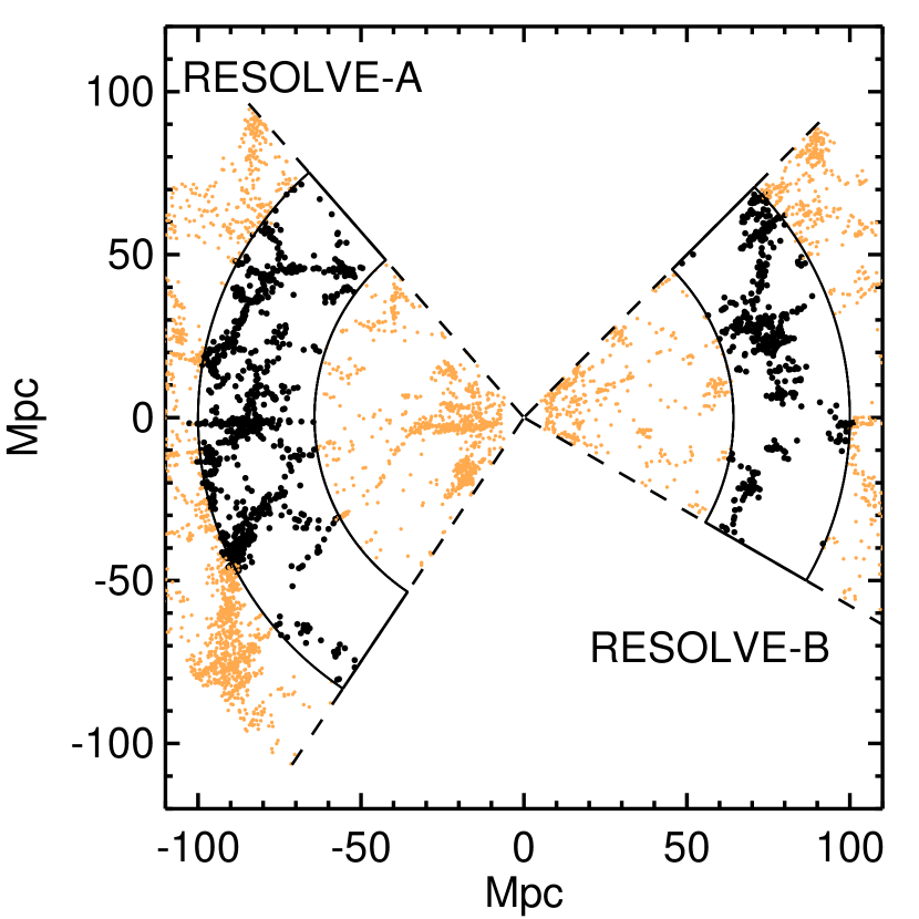
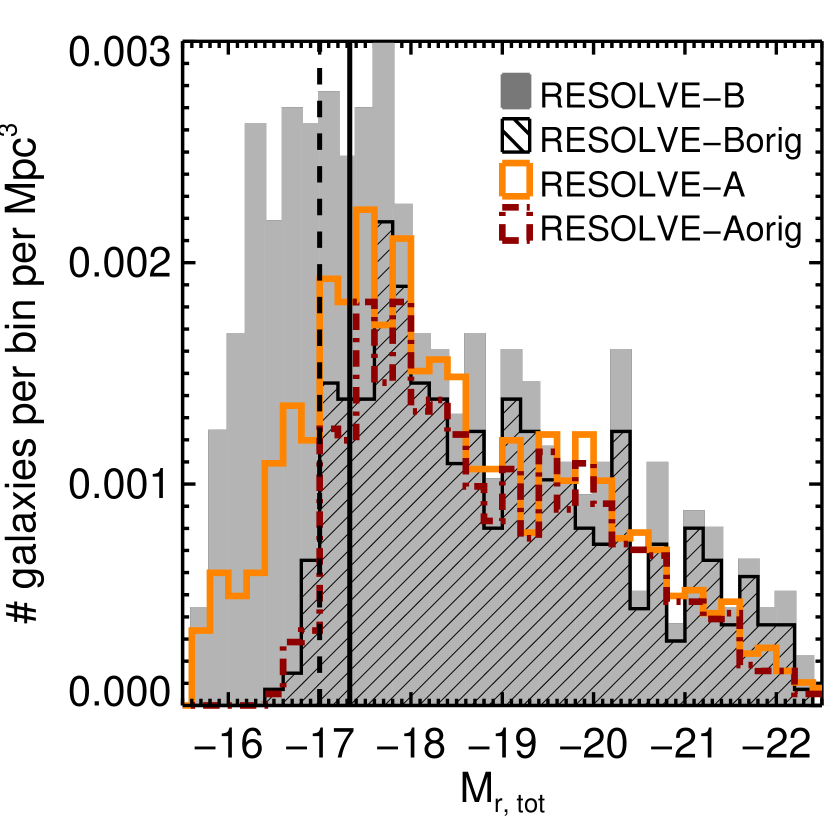
Figure 1.— RA–cz and $r$-band absolute magnitude distributions of RESOLVE-A and -B semesters. a) The regions outlined in black show the RA and cz limits of the two RESOLVE subvolumes; both have been collapsed in Dec, ranging 0–5^∘ for RESOLVE-A and $-1.25$ to +1.25^∘ for RESOLVE-B. The black dots show RESOLVE galaxies, identified as members of RESOLVE because their group redshift falls within the limits of the survey. Orange points show galaxies belonging to groups outside of the RESOLVE cz limits 4500–7000 km s^-1. b) The black hash filled histogram and red dot-dashed outlined histograms show the original absolute $r$-band magnitude distributions for RESOLVE-B and RESOLVE-A respectively. Both distributions fall off rapidly below M_r,tot $<$ $-17.33$. The grey shaded histogram and the orange solid outlined histogram show the full absolute $r$-band magnitude distributions for RESOLVE-B and RESOLVE-A after redshift completion efforts described in §2. The RESOLVE-A region is still complete only to M_r,tot = $-17.33$, however we are able to move the RESOLVE-B completeness limit down to $-17.0$.

2.1. RESOLVE-A

The RESOLVE-A data set shown in Figure 1a occupies a volume of $\sim$38,400 Mpc³ defined by: 131.25^∘ $<$ RA $<$ 236.25^∘, 0^∘ $<$ Dec $<$ 5^∘, and 4500 km s^-1 $<$ cz $<$ 7000 km s^-1. The data set’s $r$-band absolute magnitude distribution is shown in the orange solid line histogram in Figure 1b. RESOLVE-A is complete down to M_r,tot $<$ $-17.33$ using the reprocessed photometry described in §3.1. A magnitude of M_r,tot $\sim$ $-17.33$ roughly corresponds to M_bary $\sim$ 10^9.1 $M_{\odot}$ (K13). To determine the baryonic mass completeness limit, we consider the scatter in baryonic mass-to-light ratio, which can be at least as high as 3 resulting in a baryonic mass limit of 10^9.3 $M_{\odot}$. The RESOLVE-A survey contains 955 galaxies brighter than M_r,tot = $-17.33$. Of these 955 galaxies, $\sim$12% were added from redshift surveys besides the SDSS main redshift survey. The data set resulting from the SDSS main redshift survey alone (RESOLVE-Aorig) is shown as the red dot-dashed line histogram in Figure 1b. The RESOLVE-A region is 78% complete in HI when counting successful, unconfused HI detections and strong upper limits resulting in 1.4M_HI $<$ 0.05M_star. We use the RESOLVE-A data set to determine our PGF calibrations, accounting for missing HI data with an iterative Monte Carlo technique akin to survival analysis (see §4 and §6).

2.2. RESOLVE-B

The RESOLVE-B data set is located in the SDSS Stripe 82 equatorial region, and it occupies a smaller volume of $\sim$13,700 Mpc³ defined by: 22h $<$ RA $<$ 3h, $-1.25^{\circ}$ $<$ Dec $<$ 1.25^∘, and 4500 km s^-1 $<$ cz $<$ 7000 km s^-1. In Figure 1b the absolute $r$-band magnitude distribution is shown for RESOLVE-B galaxies coming from the SDSS main redshift survey as the black hashed histogram (RESOLVE-Borig), as well as for the full RESOLVE-B data set (grey filled histogram), which includes redshifts from the sources mentioned in §2 and extra SDSS redshift observations over the Stripe 82 footprint. The data set is complete in $r$-band absolute magnitude down to M_r,tot $\cong$ $-17.0$, slightly deeper than RESOLVE-A implying completeness to M_bary $\sim$ 10^9.1 $M_{\odot}$. The RESOLVE-B survey contains 487 galaxies to this limit, $\sim$25% of which have been added by redshift surveys besides the SDSS main redshift survey. We have recovered more galaxies in RESOLVE-B than in RESOLVE-A due to the extra spectroscopic passes done by the SDSS that are not part of the main SDSS redshift survey. The RESOLVE-B region is $\sim$75% complete in HI data for good HI detections and strong upper limits. We use the RESOLVE-B data set to test our new PGF calibrations and compare with other calibrations from the literature (see §7).

3. Data

For this work we need consistent and well calibrated photometry, stellar masses, and HI masses down to fixed fractional mass limits. We present our methods for reprocessing UV, optical, and IR photometry for the RESOLVE survey in §3.1. We then describe our stellar mass estimation through SED modeling in §3.2. Lastly we describe the various sources of HI data and the measurement of HI masses §3.3.

3.1. Photometric Data

We have reprocessed photometric data for the RESOLVE survey from the UV to near IR to obtain consistent, well-determined total magnitudes, and we use two to three methods of flux extrapolation per band to characterize systematic errors on the total magnitudes of the galaxies. We have also run the same pipeline on the larger volume-limited ECO (Environmental COntext) catalog (Moffett et al., submitted), which surrounds the RESOLVE-A subvolume. We use optical $ugriz$ data from SDSS (Aihara et al., 2011), NIR $JHK$ from 2MASS (Skrutskie et al., 2006) and/or $YHK$ from UKIDSS (Hambly et al., 2008), and NUV from the GALEX mission (Morrissey et al., 2007). Our NUV data are mostly MIS depth due to prioritization of the RESOLVE-A footprint late in the GALEX mission (after the FUV detector failed), while RESOLVE-B (Stripe 82) already had deep coverage in both the NUV and FUV for other programs. The SDSS optical imaging in the RESOLVE-B footprint is extra deep due to repeated imaging with typically 20 frames per location on the sky (Annis et al., 2014). With our improved photometry and realistic error measurements, we are able to measure reliable colors and perform accurate stellar mass estimation via SED modeling.

Our reprocessed photometry improves over SDSS pipeline photometry in several key ways. First, we use images with improved sky subtraction coming from either Blanton et al. (2011) for SDSS or our own additional sky subtraction for 2MASS and UKIDSS. Second, we use the sum of the high S/N $gri$ images to define the elliptical apertures, allowing us to determine the PA and axial ratio of the outer disk if present. Third, we apply these same elliptical apertures to all bands which allows us to measure magnitudes for galaxies that may not have been detected by the original automated survey pipeline in certain bands, especially low surface brightness galaxies in 2MASS, UKIDSS, and GALEX. Lastly, we use two to three non-parametric methods of total magnitude extrapolation, measuring the light from each band independently (see Figure 2 and §3.1.2). This last point allows for color gradients within galaxies, as opposed to the model magnitudes provided by SDSS (more details in §3.1.3), and allows us to measure systematic errors on magnitudes.

We provide a comparison of the magnitudes, colors, and radii with photometry from the DR7 catalog of SDSS in Figure 3 and §3.1.3. Briefly summarizing, we find that the newly reprocessed photometry yields brighter magnitudes and larger effective radii. The colors tend to be bluer for large objects, which we believe to be a consequence of both the improved sky subtraction from Blanton et al. (2011) and the fact that we allow color gradients in magnitude estimation. The newly reprocessed photometry does not create a tight red sequence on the color-magnitude relation as seen in the DR7 photometry, however we argue that the tight red sequence may be a consequence of these two issues in §3.1.3. We also discuss an independent validation of our methods with the NFGS survey (shown in Figure 2a of K13) in §3.1.3.

In addition to the reprocessed photometry, this paper also presents new UV observations of 19 galaxies using the Swift Ultraviolet/Optical Telescope (UVOT, Roming et al., 2005, see also Gehrels et al., 2004). We use imaging from the uvm2 filter, which has a comparable central wavelength but narrower width than the GALEX NUV filter (see Poole et al., 2008). Compared to GALEX, the pointing restrictions for UVOT are much less stringent, allowing us to obtain observations during Swift team fill-in time for RESOLVE-B galaxies that were not observed by GALEX or had only AIS depth ($\sim$150s) coverage. Nineteen galaxies were observed for more than 1 ks, the minimum exposure for useful photometry. Images were processed following Hoversten et al. (2011). Each galaxy was manually inspected to make sure that the surface brightness in the uvm2 band was low enough that the resulting photometry errors due to coincidence loss were below 1% (see Poole et al., 2008; Breeveld et al., 2010; Hoversten et al., 2011). We apply similar photometric processing to the Swift data as to the archival data including matched elliptical apertures and multiple extrapolation techniques.

3.1.1 Custom Processed Data

We start the photometric reprocessing by downloading the data from each respective website, performing background subtraction and coaddition when necessary, and cropping a region around the galaxy 9 times the Petrosian 90% light radius as reported by SDSS with a minimum crop size of 3x3 arcmin². Because some galaxies are quite large, we rescale images to a fixed image size, causing the pixel scale to vary from galaxy to galaxy. Since the Stripe 82 region has been repeatedly observed in $ugriz$, for RESOLVE-B galaxies we coadd the many frames of data by inversely weighting by the variance of sky fluctuations using the IRAF task imcombine. Within the RESOLVE-A region there is typically one $ugriz$ frame per region of sky, and we use SWARP (Bertin et al., 2002) to stitch together adjacent frames when necessary, averaging together pixels where there is overlap between images. No additional background subtraction is done, as we are using SDSS DR8 images with the optimized sky background subtraction of Blanton et al. (2011). For 2MASS $JHK$ and UKIDSS $YJHK$, we perform additional background subtraction by fitting and subtracting a 3rd order polynomial to a region of the galaxy frame where the galaxy and other objects are masked out. Coaddition is similar to the single frame SDSS process, using SWARP to stitch together 2MASS and UKIDSS frames with a simple average to combine pixels in overlapping areas of the sky. Based on visual inspection of the UKIDSS data, we do not use the $J$ band due to background subtraction and other issues that affect $\sim$75% of the data. We have also examined the $YHK$ images for each galaxy by eye to flag any cases with bad data. The GALEX NUV images do not require additional background subtraction, and these images are simply coadded using SWARP and weighted by exposure time. For the Swift uvm2 images we use Source Extractor to identify and mask objects within the frame, then subtract off the median level of the non-masked areas as the sky-background.

A significant number of galaxies ($\sim$16%) in RESOLVE have half-light diameters smaller than three times the typical $r$-band psf FWHM of $\sim$$1.4$″, warranting psf-matching across the optical bands and UKIDSS IR bands. For each galaxy, we use the SDSS provided psField frame to reconstruct the psf for each band at the galaxy position on the frame. First we identify the band with the worst psf seeing (typically $u$ or $g$). Next we find the Gaussian $\sigma$ value with which to convolve the psf of each given band to eliminate the difference between the psf of the worst band and that given band. This Gaussian $\sigma$ value is then used to create a Gaussian kernel that is convolved with the galaxy cropped image. Since we have changed the pixel scale of the frames of larger galaxies, we make sure to convert the $\sigma$ value into the correct pixel scale for that galaxy. For UKIDSS IR data a similar procedure is run, except that the psf for each frame is constructed from stars identified by Source Extractor. If the value of the converted $\sigma$ value is less than one pixel, we do not perform the convolution. We do not psf-match the NUV, uvm2, or 2MASS $JHK$ bands because their typical psfs are much larger than the SDSS ($\sim$5.5″ for NUV, $\sim$2.5″ for uvm2, and $\sim$2″ for 2MASS). Thus aperture matched magnitude measurements for the UV and 2MASS IR will not be correct, especially for small galaxies.

Masks are made from the $r$-band image using Source Extractor (Bertin & Arnouts, 1996) to detect stars and galaxies other than the target. Masks are checked by eye to ensure there is no under/over masking. In §3.1.3 we discuss the application of this photometric reprocessing pipeline for the ECO (Environmental COntext) catalog (Moffett et al., submitted), for which we do not check each mask by eye. Instead we use a first iteration of the pipeline to check for discrepant total and aperture magnitudes as well as cases with no valid magnitudes at the end. For the most egregious outliers, we check the masks and edit by hand where necessary.

To determine the parameters of the elliptical fit (namely the PA and ellipticity), we use an iterative procedure involving two programs. First, Source Extractor is run on each galaxy’s cropped $r$-band frame to find an initial guess for the center, PA, and ellipticity, and 90% light radius. Second, we run the IRAF task ellipse on the $gri$ coadded image using the Source Extractor quantities as inputs and allowing the PA and ellipticity, but not the center, to vary. The $gri$ images have the highest signal-to-noise data, and by coadding these three bands, we provide the best image to feed to ellipse for determining the PA and ellipticity in the the outer parts of the galaxy. The final PA and ellipticity are chosen using a median of the fits from the outer disk of the galaxy, where “outer disk” is defined between one and two times the 90% $r$-band light radius determined by Source Extractor. Using the final PA, ellipticity and galaxy center, we then perform a fixed ellipse fit on the $gri$ summed image to determine the set of annuli over which to measure the galaxy surface brightness profiles for each band separately.

These same annuli are then automatically applied to the GALEX, SDSS, 2MASS, and UKIDSS data. To match the NUV and $YJHK$ images to the SDSS images, we resample them to the pixel scale of the SDSS image. Imposing the same annuli over all bands allows us to measure the galaxy light out to its furthest extent (based on $gri$). For the IR bands, we are able to measure magnitudes for twice as many galaxies as the 2MASS catalog detects and for $\sim$1.15 times as many galaxies as the UKIDSS catalog (based on public DR8plus).

Some galaxies are in very close pairs or embedded within a larger galaxy. To obtain better photometry for these galaxies, we have attempted to subtract off the galaxy light from the interfering galaxy for each frame, when it seems possible to identify the light belonging to a specific galaxy. To flag such cases we search for whether a nearby galaxy is within 4 times the 50% $r$-band light radius of each RESOLVE galaxy. This selection returns 27 systems. We inspect these 27 systems and remove 11 which appear well separated from their neighbors. We also remove three closely paired systems (rs1158/rs1160, rs0100/rs0101, rs0196/rs0197), two that involve merging star forming spirals and one that contains two similarly sized elliptical galaxies, all three of which are so close as to make it impossible to disentangle the light from each galaxy. We find 13 systems that benefit from attempting to remove the light from a galaxy.

Embedded Galaxies: There are five systems that are heavily embedded inside a much larger galaxy: rs0675, rs0749, rs1233, rs1227, and rs0072 (inside rs0673, rs0750, rs1232, rs1226, and rs0072 respectively). Another three systems are on the outskirts of a larger galaxy: rs0639, rs1089, and rf0090 (just outside of rs0642, rs1090, and rf0094 respectively). To obtain better photometry for these eight embedded galaxies, we first mask the small embedded galaxy and run ellipse on the larger galaxy. We then subtract off the model flux from the larger galaxy that is output from ellipse. We use the resulting image that has the large galaxy subtracted out to run through the procedures described in this section, ensuring that any residuals from the model are masked out.

Close Pairs: There are five close pair systems for which subtracting off the light of one or both of the members improves the magnitude estimates. These systems are rs0267/rs0268, rs0397/rs0398, rs0851/rs0852, rf0015/rf0016, and rf0309/rf0310. To subtract off the light of each member we use the following steps:

• First, we identify the galaxy with the simpler light profile, which we call galaxy-A. For each pair galaxy-A is rs0268, rs0397, rs0851, rf0016, and rf0310.

• Second, we start with the image for the other galaxy, which we call galaxy-B. We mask galaxy-B and run ellipse to fit the light profile of galaxy-A.

• Third, we subtract off the galaxy-A model flux as provided by ellipse from the galaxy-B image. The resulting image is used in the standard pipeline for galaxy-B (rs0267, rs0398, rs0852, rf0015, rf0309).

• In most cases, we do not then subtract off the galaxy-B image for galaxy-A. We choose not to for a variety of reasons. For rs0267/rs0268, galaxy-B (rs0267) does not have a regular light profile making it difficult to subtract off. For rs0397/rs0398 and rf0309/rf0310 galaxy-B (rs0398, rf0310) is edge-on and easy to mask. For rs0851/rs0852, galaxy-B (rs0852) is much smaller and easier to mask out.

• For the last pair rf0015/rf0016, we take the galaxy-B (rf0015) image with galaxy-A’s light subtracted off and mask any residuals from galaxy-A. We run ellipse to fit the light profile of galaxy-B. We then subtract off the model fit to galaxy-B provided by ellipse from the original galaxy-B image. The resulting image of galaxy-A (which is no longer in the center) is run through the pipeline with newly generated masks.

We perform these procedures for all optical bands and UKIDSS images. For 2MASS and GALEX, we check first whether the subtraction is needed because the galaxy light may not extend far enough in these bands.

3.1.2 Magnitude Extrapolation

To extrapolate total magnitudes from the fixed ellipse fits for the optical bands, we use three methods: an exponential (Sersic index $n=1$) fit to the outer disk, a non-parametric Curve of Growth extrapolation, and an Outer Disk Color Correction based on the $r$-band. Figure 2 shows schematics of all three methods in the $g$ band for a RESOLVE-B galaxy.

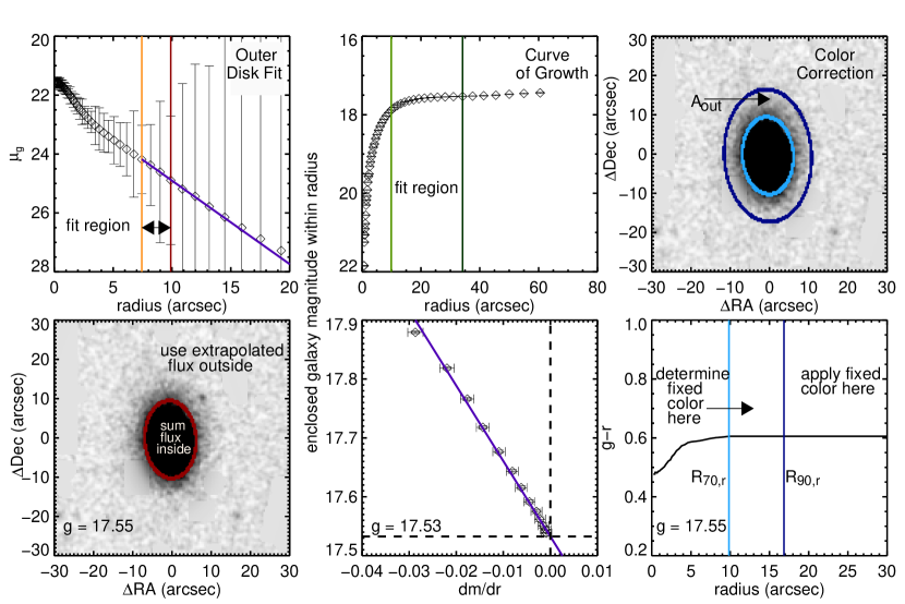
Figure 2.— Illustration of the three methods described in §3.1.2 to extrapolate the total $g$-band magnitude for RESOLVE-B galaxy rf0218. In this case, all three estimates agree closely (17.55, 17.53, 17.55), yielding a small systematic error (0.021). Left column: To demonstrate the Outer Disk Fit method, we show in the top left panel annular $g$-band surface brightness vs. radius with the fitting region marked by the orange (inner) and red (outer) lines. The blue line shows the exponential disk fit to the data points. The bottom left panel illustrates how we compute the total magnitude as the sum of the raw galaxy flux inside the radius marked by the red line (same as radius in top panel marked by red line) and the extrapolated flux outside that radius. Middle column: To demonstrate the Curve of Growth method, we show in the top middle panel enclosed galaxy magnitude vs. radius with the fitting region marked by light green (inner) and dark green (outer) lines. The lower middle panel shows the enclosed galaxy magnitude vs. the derivative of enclosed magnitude with respect to radius for the points within the fitting region defined above. The blue line shows the fit and the y-intercept at dm/dr = 0 is the total galaxy magnitude. Right column: To demonstrate the Outer Disk Color Correction method, we show in the top right panel the annulus A_out defined by the $r$-band 70% and 90% light radii (light and dark blue lines respectively). Using the flux ratio in A_out, we fix the color of the galaxy to determine the $g$-band flux beyond $R_{90,r}$, from the $r$-band flux in that region.

Outer Disk Fit: To compute the outer disk flux, we first define a fitting region where the annular flux is 1 to 5 times the $\sigma$ of the sky noise. If the galaxy frame has been masked heavily (due to nearby stars or galaxies), we use a region 3 to 8 times the $\sigma$ of the sky noise, and in extreme cases where a bright star or galaxy is on top of the galaxy, we use a region defined by 20-50 times the $\sigma$ of the sky noise. Then we fit an exponential disk function to the fitting region of the galaxy surface brightness profile (between orange and red lines in left panel of Figure 2) and sum the extrapolated flux from the inner edge of the last ellipse in the fitting region (red line) to an extremely large radius “$R_{\infty}$” or 1000″ past the inner edge of the last ellipse in the fitting region (red line). To compute the inner disk flux, we sum the raw, unmodeled flux interior to the inner edge of the last ellipse in the fitting region (red ellipse in left panels of Figure 2). If pixels are masked in the raw data, we replace those values with the model output from ellipse. The exponential total magnitude equals the sum of the measured inner flux and the extrapolated outer disk flux. The typical dividing radius is near the 90% light radius in the $r$ band.

Curve of Growth: The Curve of Growth method, following Muñoz-Mateos et al. (2009), computes the total magnitude using the derivative of the enclosed magnitude as a function of the radius. The enclosed magnitudes are calculated from the ellipse profile. A line is then fitted to the derivative of enclosed magnitude with respect to the radius vs. the total enclosed magnitude. The line is fitted over a new fitting region that extends farther out in the galaxy profile, to where changes in the total enclosed magnitude as a function or radius are small (between the light and dark green lines in the central panel of Figure 2). The y-intercept of the fitted line, where dm/dr = 0, is the total Curve of Growth magnitude.

Outer Disk Color Correction: This method scales the outer disk $r$-band flux to determine the outer disk flux of an object in another band. First, we use either the Curve of Growth or the Outer Disk Fit $r$-band magnitude to determine the radii containing 70% and 90% of the $r$-band light in the running total flux profile (light and dark blue ellipses show these respective radii in right most panel of Figure 2). If the galaxy frame is heavily masked (more than 5% of the image pixels), we prefer the $r$-band exponential magnitude, otherwise the $r$-band Curve-of-Growth magnitude is used. We next measure the galaxy flux within the $R_{70,r}$ to $R_{90,r}$ annulus (A_out). If the S/N of the flux in this annulus is not greater than 10, we decrease the inner radius of A_out by increments of 5% down to 50% of the $r$-band light, stopping when we achieve S/N $>$ 10. If the S/N is still less than 10 between $R_{50,r}$ and $R_{90,r}$, we do not compute the galaxy magnitude with this method. Otherwise, we calculate the flux ratio between a given band $x$ and the $r$ band within the annulus A_out, and we assume that this ratio continues out to infinity. From the $r$-band flux from $R_{90,r}$ to $R_{\infty}$, and the flux ratio within A_out, we estimate the flux in band $x$ from $R_{90,r}$ to $R_{\infty}$, then add this flux to the raw enclosed flux inside $R_{90,r}$ to get the final magnitude.

Extrapolation of the NIR and UV magnitudes proceeds similarly to the optical extrapolation, but with a few subtleties. The Curve of Growth method is the preferred method for our NIR data due to the poor signal-noise for low surface brightness galaxies. Exponential fits are used to determine whether or not the Curve of Growth method works well. If the two fits disagree significantly or if the object’s magnitude is very faint, we look at the magnitude calculated based on the $i$ band (using the Outer Disk Color Correction method). If either the Curve of Growth or exponential matches the aperture magnitude, that is chosen. If neither method agrees, the Outer Disk Color Correction is used and given a large systematic error ($>$0.5 mag). For the UV data from both GALEX and Swift, we find that the Curve of Growth method is the most reliable magnitude estimation method as the clumpiness of the UV and the possibility of XUV disks (extended UV emission outside the typical optical extent of the galaxy; Thilker et al., 2007) make exponential disk fitting and fixing the outer disk color impractical. The Outer Disk Color Correction method is also hampered by the mismatch in psf between the UV images ($\sim$5.5″ and $\sim$2.5″ for the NUV and uvm2 respectively) and the psf of the convolved SDSS and UKIDSS images ($\sim$1.8″). If the Curve of Growth method fails, though, we use the magnitude of the Outer Disk Color Correction method, with a systematic error $>$ 0.06 applied.

Errors for all bands are computed using not only the formal statistical error on the magnitude, but also the systematic error based on the difference in flux measured from the three methods. We apply a built in floor for the systematic error based on the overall distribution of systematic errors for the galaxy data set, such that none are lower than the original 25 percentile.

In addition we compute half light and 90% light radii in the $r$ band ($R_{50,r}$ and $R_{90,r}$), as well as the $r$-band surface brightness within these radii ($\mu_{r,50}$ and $\mu_{r,90}$). We also measure aperture magnitudes for all available bands within the $r$-band half light and 90% light radii, although the lack of psf correction for the 2MASS $JHK$ and NUV and uvm2 bands compromises associated aperture matched colors. We also compute the $g-r$ color gradient (hereafter $\Delta_{g-r}$), which is defined as the $g-r$ color within the annulus between the half light and 75% $r$-band light radii minus the $g-r$ color within the $r$-band half light radius. More positive colors indicate galaxies with bluer centers.

Throughout this work we use Milky Way foreground extinction corrections determined from the dust maps of Schlegel et al. (1998) with the extinction curves of O’Donnell (1994) for the optical and IR data, and of Cardelli et al. (1989) for the NUV and uvm2 data. For the NUV and uvm2 data we use the extinction correction calculated at 2271 Å and 2221 Å, the effective wavelengths of the NUV and uvm2 filter respectively. We note that using the more recently computed extinction coefficients from Schlafly & Finkbeiner (2011), which use the extinction curve from Fitzpatrick (1999), yields colors that are $\sim$0.015 mag bluer in $u-r$ ($\sim$0.04 bluer in NUV$-r$) and do not change the stellar mass estimates from §3.2.

Table 1 provides descriptions of the columns that are provided in a machine readable table with the photometry for the RESOLVE survey. All galaxies processed are provided, including those in the buffer and fainter than the nominal RESOLVE limits.

Table 1RESOLVE Custom Photometry Catalog Description

Column	Description
1	RESOLVE ID
2	Right Ascension
3	Declination
4	cz
5	group cz
6	absolute SDSS $r$-band magnitude
7	apparent SDSS $u$-band magnitude
8	apparent SDSS $u$-band magnitude error
9	apparent SDSS $g$-band magnitude
10	apparent SDSS $g$-band magnitude error
11	apparent SDSS $r$-band magnitude
12	apparent SDSS $r$-band magnitude error
13	apparent SDSS $i$-band magnitude
14	apparent SDSS $i$-band magnitude error
15	apparent SDSS $z$-band magnitude
16	apparent SDSS $z$-band magnitude error
17	apparent GALEX NUV-band magnitude
18	apparent GALEX NUV-band magnitude error
19	apparent Swift uvm2-band magnitude
20	apparent Swift uvm2-band magnitude error
21	apparent 2MASS $J$-band magnitude
22	apparent 2MASS $J$-band magnitude error
23	apparent 2MASS $H$-band magnitude
24	apparent 2MASS $H$-band magnitude error
25	apparent 2MASS $K$-band magnitude
26	apparent 2MASS $K$-band magnitude error
27	apparent UKIDSS $Y$-band magnitude
28	apparent UKIDSS $Y$-band magnitude error
29	apparent UKIDSS $H$-band magnitude
30	apparent UKIDSS $H$-band magnitude error
31	apparent UKIDSS $K$-band magnitude
32	apparent UKIDSS $K$-band magnitude error
33	$b/a$ axial ratio of outer disk
34	$R_{50,r}$ half-light radius in $r$ band
35	$R_{90,r}$ 90% light radius in $r$ band
36	$\Delta_{g-r}$ $g-r$ color gradient
37	$(u-r)^{m}$ modeled $u-r$ color
38	$(u-i)^{m}$ modeled $u-i$ color
39	$(u-J)^{m}$ modeled $u-J$ color
40	$(u-K)^{m}$ modeled $u-K$ color
41	$(g-r)^{m}$ modeled $g-r$ color
42	$(g-i)^{m}$ modeled $g-i$ color
43	$(g-J)^{m}$ modeled $g-J$ color
44	$(g-K)^{m}$ modeled $g-K$ color
45	stellar mass
46	foreground extinction in $u$ band
47	foreground extinction in $g$ band
48	foreground extinction in $r$ band
49	foreground extinction in $i$ band
50	foreground extinction in $z$ band
51	foreground extinction in NUV band
52	foreground extinction in uvm2 band
53	foreground extinction in $Y$ band
54	foreground extinction in $J$ band
55	foreground extinction in $H$ band
56	foreground extinction in $K$ band

Note. — All magnitudes are newly measured from the raw images. Apparent magnitudes are provided without foreground extinction corrections. Foreground extinction corrections used in this work are provided. Modeled colors designated by a superscript m are products of the SED fitting routine from K13, described in §3.2 and have foreground extinction corrections and k-corrections implicitly included. The datatable is provided at http://resolve.astro.unc.edu/data/resolve_phot_dr1.txt

3.1.3 Comparison with Catalog Photometry

We compare our newly reprocessed magnitudes, radii, and colors to the Petrosian and model photometry provided in the SDSS DR7 catalog in Figure 3. SDSS catalog Petrosian magnitudes are measured within a circular aperture of twice the Petrosian radius, defined as the radius $R_{p}$ where the ratio of the local surface brightness at $R_{p}$ to the surface brightness within $R_{p}$ is equal to 0.2 (Blanton et al., 2001). The SDSS pipeline uses the Petrosian radius defined by the $r$ band to compute Petrosian magnitudes for all other bands, thus yielding aperture-matched magnitudes and colors. The Petrosian system should pick up nearly total fluxes for disk (Sersic $n=1$) galaxies, but is known to underestimate magnitudes for higher Sersic $n$ galaxies by $\sim$0.2 mag (Graham et al., 2005). The SDSS pipeline also computes model magnitudes by fitting exponential ($n=1$) and de Vaucouleurs ($n=4$) models to the galaxy light profile, choosing the model of greater likelihood in the $r$ band, and extrapolating the profile to infinity. To measure model magnitudes for the $ugiz$ bands, the SDSS pipeline scales the amplitude of the $r$-band profile up or down to best match the profile in that band (Stoughton et al., 2002). Neither magnitude system is ideal as the Petrosian magnitudes do not measure the total galaxy light, while the model magnitudes are most sensitive to the inner profile of the galaxy and do not allow for color gradients within galaxies.

In Figure 3a we compare our newly reprocessed $r$-band magnitudes with DR7 Petrosian catalog magnitudes as a function of galaxy half light radius $R_{50,r}$. The reprocessed $r$-band magnitudes are overall brighter by $\sim$0.13 mag than the DR7 Petrosian $r$-band magnitudes. We find a similar, but slightly smaller, overall offset of $\sim$0.1 mag between our newly reprocessed magnitudes and the DR7 model $r$-band magnitudes. The offset increases for the largest galaxies, as seen in the running median as a function of $R_{50,r}$ (black dashed line, Figure 3a). Much of this trend can be attributed to our use of the improved sky background subtraction from Blanton et al. (2011), which was not available for DR7. The blue solid line shows the expected median offset between galaxy magnitudes using the new sky subtraction vs. the standard SDSS DR7 pipeline, as a function of true galaxy $R_{50,r}$ (based on coefficients from Table 1 of Blanton et al. 2011, only valid for $R_{50,r}$ $>$ 5″). Our running median matches very well with the expected trend. Note also that in this work, we do not use information from the inner profile of the galaxy to compute extrapolated total magnitudes, but rather extrapolate the light based on the outer profile of the galaxy. This difference may also contribute to the generally brighter magnitudes that we measure.

In Figure 3b we compare our newly remeasured $R_{50,r}$ values with DR7 catalog $R_{50,r}$ values as a function of the newly remeasured $R_{50,r}$. Since we measure greater flux per galaxy, we expect the half-light radii to be larger, and indeed we find that the new $R_{50,r}$ values are typically $\sim$49% larger than the SDSS Petrosian $R_{50,r}$ values and $\sim$13% larger than the model $R_{50,r}$ values. The ratio between the new and catalog $R_{50,r}$ values becomes much greater above a remeasured $R_{50,r}$ of $\sim$10″, the value identified by Blanton et al. (2011) as the true galaxy half light radius above which the use of the new sky background should significantly affect the measured galaxy flux and radius measurement. Another consideration affecting only the Petrosian radii is the fact that SDSS Petrosian apertures are circular whereas both our apertures and SDSS model apertures are elliptical. When we restrict the comparison of half light radii to galaxies with $b/a$ $>$ 0.85, our half light radii are only $\sim$20% larger than the Petrosian radii, more in line with the 13% increase over the model radii. Figure 9 of Hall et al. (2012) also shows the trend for Petrosian half light radii to have greater disagreement with remeasured half-light radii for more intrinsically edge-on galaxies.

Figure 3.— Comparison of newly reprocessed photometry and SDSS DR7 photometry. a) Comparison of absolute Petrosian magnitudes M_r,petro and absolute total magnitudes M_r,tot from this work as a function of remeasured $R_{50,r}$. Our reprocessed photometry is brighter than the SDSS DR7 catalog Petrosian photometry; the running median is shown as a dashed black line. (We observe similar but slightly smaller offsets between our reprocessed photometry and the SDSS DR7 catalog model photometry.) The solid blue line shows the expected magnitude difference using the new sky subtraction vs. the SDSS standard pipeline as a function of true galaxy $R_{50,r}$, based on the analysis of Blanton et al. (2011), which is in excellent agreement with our data. b) Comparison showing $R_{50,r}$ from our reprocessed photometry divided by $R_{50,r}$ from the DR7 photometry (Petrosian: black dots; model: pink squares), as a function of the new $R_{50,r}$ in arcsec. The green solid line shows one-to-one correspondence, and the green dashed line marks 10″, above which the new background subtraction should significantly affect the measured flux and radius of the galaxy (Blanton et al., 2011). Our newly reprocessed photometry yields $\sim$13% larger half-light radii than SDSS model half-light radii, with larger increases for galaxies with $R_{50,r}$ $>$ 10″. The increases over Petrosian radii are more extreme due to the assumption of circularity in the Petrosian algorithm.

In Figure 4 we compare the newly reprocessed total $u-r$ colors and the DR7 model $u-r$ colors vs. M_r,tot. We find that the new $u-r$ colors are overall $\sim$0.18 mag bluer than the DR7 model $u-r$ colors. To compute this offset, we measure the running medians of each color distribution as a function of M_r,tot in 0.2 mag bins and subtract the two sets of median colors. We then determine the median of these median color differences, which is 0.18 mag. A large portion of the offset is due to the improved sky subtraction algorithm, but we also note the fact that our newly reprocessed photometry allows for color gradients whereas SDSS model colors do not. Galaxy color gradients have been found in all galaxy types (e.g., de Jong, 1996; Jansen et al., 2000; Cibinel et al., 2013). For example in the Nearby Field Galaxy Survey, Jansen et al. (2000) find that early and late types have typical $B-R$ colors that are bluer by 0.1-0.2 mag in their outer regions, while dwarf types distribute evenly between blue and red color gradients. In this work we have explicitly allowed for color gradients by computing the total magnitudes in each band separately without the assumption of fixed profile shape built into the SDSS model magnitude algorithm. Even the Outer Disk Color Correction method fixes only the color outside the A_out annulus.

A consequence of ignoring color gradients is that the red sequence defined by DR7 model $u-r$ colors appears tighter than the red sequence defined by our newly reprocessed $u-r$ colors. To quantify the scatter, we fit a line to both sets of colors between the red sequence boundaries marked off by the red lines in Figure 4, and measure the rms from the fit. The red sequence definition is shifted for the newly reprocessed $u-r$ colors by 0.18 mag to account for their overall bluer colors. We confirm the visual impression that the DR7 red sequence is tighter, finding that the SDSS model $u-r$ red sequence is tighter by $\sim$16%. This tight red sequence seems to be an artifact of the SDSS model magnitude algorithm and should not be over-interpreted in measuring the star formation histories of red sequence galaxies. We note that Simard et al. (2011) also report that using separate fits to compute $g$- and $r$-band magnitudes produces a more scattered red sequence than obtained when fixing fits in both bands to have the same half light radius, although these authors still choose fixed half light radius fits for convenience.

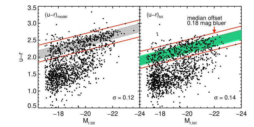
Figure 4.— Comparison of $u-r$ color vs. our M_r,tot for DR7 model colors (left) and our newly reprocessed colors (right). We determine the red sequence boundaries (red lines) for the DR7 data by eye, throwing out outliers that are too red. We then fit a line to the data points between the two red lines and compute the rms which is 0.12 for the DR7 model magnitudes (slope and width of red sequence shown by grey has marked region). To do the same for the newly reprocessed photometry, we first determine the overall color offset by computing the median color of each distribution in bins of 0.2 mag in M_r,tot. We then find the median of the differences of the medians in each bin, obtaining an overall shift of 0.18 mag. We shift down our red sequence boundaries by 0.18 mag for the newly reprocessed photometry. We then fit a line and compute the rms to be 0.14 mag (slope and width shown in green solid region with slope and rms of DR7 model colors shifted down by 0.18 mags and overplotted), which is larger by 0.02 mag or 15% than the rms computed for the DR7 colors. As argued in §3.1.3, we believe the higher scatter in our red sequence to be more correct, as our photometry does not suppress color gradients. Also most of the few extremely red outliers (including one at $u-r$_tot = 3.6 off the plot) are low surface brightness red galaxies whose shallow $u$ band data are the hardest to measure. A few others are those embedded galaxies for which we subtracted off the light of the larger galaxy.

In Figure 5 we compare independent photometric measurements for RESOLVE survey galaxies that overlap with the ECO (Environmental COntext) catalog (Moffett et al., submitted), which is a larger volume-limited data set encompassing the RESOLVE-A subvolume. The ECO catalog has been reprocessed through the same pipeline, with the most significant difference in methodology occurring at the masking step. Since ECO has $\sim$10 times the number of galaxies as RESOLVE, for ECO it was not feasible to check each mask by hand. The most egregious cases of over- or under-masking were determined in a preliminary run of the photometry code on the catalog, by checking for extrapolated magnitudes that significantly disagreed with aperture magnitudes or cases where no magnitude was measured. The masks for these galaxies were then checked by eye to mitigate under-/over-masking. We compare the ECO and RESOLVE M_r,tot measurements for galaxies in the overlapping subvolume in Figure 5a. We find no offset and only small differences of typically $<$0.2 mag between the two sets of magnitudes. Some of these differences may be attributed to the final magnitude chosen by the pipeline (Outer Disk Fit or Curve of Growth for the $r$ band), which is based on the degree to which the frame is masked. Figure 5b shows the color-magnitude plots for both the full RESOLVE-A and RESOLVE-B (blue points) and ECO (orange-red contours) data sets, demonstrating that they are consistent.

Figure 5.— Comparison of photometric measurements for galaxies in both the RESOLVE survey and the ECO catalog. a) Difference in M_r,tot measured for the same galaxies in RESOLVE-A and ECO vs. the RESOLVE-A M_r,tot. The main difference between the two measurements arises in the masking step. Every RESOLVE-A galaxy mask is checked by eye, but for the much larger ECO data set we check only images for which we have identified large discrepancies between extrapolated and aperture magnitudes. The two sets of measurements agree well, with differences mostly $<$0.2 mag. Differences become larger for fainter galaxies, for which we expect larger uncertainties in extrapolation. b) Color-magnitude relations of the full ECO (contours) and RESOLVE (dots) data sets, show that they are consistent. While we do not use ECO in this work, the ECO catalog an extension of the RESOLVE survey, so it is useful to establish that its photometry is consistent with the rest of RESOLVE.

An independent validation of the methods used in this work is shown in Figure 2a of K13 for the Nearby Field Galaxy Survey (Jansen et al., 2000). All NFGS galaxies with available SDSS data were reprocessed through the same pipeline as described here and Figure 2a in K13 shows that the reprocessed $u-r$ colors are consistent with the expected Vega-AB offset for $U-R$ colors measured in Jansen et al. (2000) over all angular sizes. The comparison between the total $u-r$ color and the SDSS DR7 model $u-r$ colors reveals an offset such that the new photometry yields $\sim$0.2 mag bluer $u-r$ colors than the DR7 model colors, similar to the offset that we measure.

3.2. Stellar Masses

Stellar masses and k-corrected colors are calculated using the spectral energy distribution (SED) modeling code described in Kannappan & Gawiser (2007), as modified by K13, which fits a grid of stellar population models to our newly reprocessed total NUV$ugrizYJHK$ magnitudes plus new Swift uvm2 data for 19 galaxies). With photometric data from up to 10 bands, we are able to estimate robust stellar masses. We omit UKIDSS $YHK$ values if the frames have been flagged by eye. We also omit UKIDSS $HK$ and 2MASS $JHK$ if the values are fainter than 18, 17.5 and 16, 15, 14.5 respectively. We also remove any NUV magnitudes fainter than 24, and we remove the $u$ band magnitudes for four galaxies for which the $u$ band data available from SDSS are essentially frames of noise.

In this work use the second model grid from K13, which is a grid of composite stellar population models (CSPs) including an old simple stellar population (SSP) ranging in age from 2-12 Gyr and a young population either described by continuous star formation starting 1015 Myr ago and turning off between 0 to 195 Myr ago or as a quenching burst with SSP age 360, 509, 641, 806, or 1015 Myr. The contribution from the young population ranges from 1-94.1% of the stellar mass. The model grid is built using the stellar population models from Bruzual & Charlot (2003) with a Chabrier IMF (Chabrier, 2003), and four possible metallicities (Z = 0.004, 0.008, 0.02, or 0.05). Eleven reddening values ($\tau$v ranges from 0–1.2) are applied to the young population following the dust extinction law given by Calzetti (2001). There is no physical or spatial model assumed for the dust, only an empirical determination of the amount of reddening and extinction based on the stellar population model grid fits to the galaxy SED.

To determine a galaxy’s stellar mass, the stellar mass is computed for each CSP model in the grid and given a likelihood based on the $\chi^{2}$ value of the model fit to the data. Combining likelihoods over all models yields a stellar mass likelihood distribution for each galaxy. The median value of this stellar mass likelihood distribution is taken to be the nominal stellar mass of the galaxy.

The SED modeling code also outputs the likelihood weighted colors for each galaxy, which are effectively “smoothed” by the model fits and implicitly k-corrected. We denote the use of these modeled colors with a superscript $m$ (following the notation from K13 and Moffett et al., submitted). The stellar population code also outputs de-extincted galaxy magnitudes, taking into account the internal extinction due to dust in the galaxy. These magnitudes cleanly divide the red and blue sequences in the color-stellar mass diagram as shown in K13 and Moffett at al., submitted. Here, however, we choose to use the modeled colors, which represent the actual rest-frame colors of the galaxies, for easier application of the PGF calibrations to other data sets. We show the color-stellar mass diagram for RESOLVE-A and RESOLVE-B using both $u-r$ total colors measured from the raw reprocessed photometry and $(u-r)^{m}$ colors from the model fits in Figure 6. The SED modeled colors agree with the measured colors well within the expected k-correction values at these redshifts of up to 0.03 mag for the $r$ band and 0.1 mag for the $u$ band.

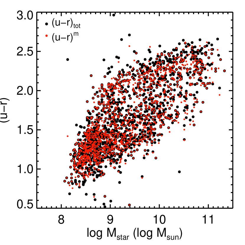
Figure 6.— Color vs. stellar mass for the entire RESOLVE survey. Black dots show total reprocessed magnitudes $u-r$ and smaller red dots show the SED modeled colors $(u-r)^{m}$. While there are outliers in the reprocessed photometry as seen in Figure 4, the SED modeled colors use information over the entire NUV$ugrizYJHK$ SED and provide a cleaner color-mass plot.

Since some stellar mass estimation techniques have been shown to be biased as a function of inclination (Maller et al., 2009), it is important to test whether our stellar masses may be biased as a function of axial ratio. We perform two tests. First, we select only galaxies with gas-to-stellar mass ratio $>$ 0.1, implying significant gas and thus potentially dust, and we divide this subset into quartiles based on their axial ratio. A KS test reveals that the stellar masses of the upper and lower quartiles ($b/a$ $>$ 0.77 and $b/a$ $<$ 0.39) are consistent with being drawn from the same population ($p_{null}=0.99$). Second, we recompute our stellar masses applying the dust law to both the young and old populations (as opposed to just the young population as for our preferred mass estimates). We find a tiny overall offset for late type galaxies of $\sim$0.02 dex but no systematic trend between the two stellar mass calculations as a function of axial ratio. For early type galaxies we find a tiny differential systematic offset of 0.02 dex between the most elongated and roundest galaxies. Both of these tests suggest our stellar mass calculations are not biased by dust extinction.

3.3. HI Masses

The HI masses and upper limits for RESOLVE come from the blind 21cm ALFALFA survey (Haynes et al., 2011) and our own new observations with the GBT and Arecibo telescopes. It is important for creating a gas mass estimator to have complete HI data for the entire data set. Below we describe the observations taken to date, how we determine and handle confused sources, and the HI completeness of the RESOLVE data set.

The ALFALFA survey has covered the entire RESOLVE-A region and the Dec 0^∘ to +1.25^∘ strip of RESOLVE-B, providing HI detections or upper limits (not necessarily strong) for 85% of RESOLVE. Data reduction and source extraction are described in Haynes et al. (2011). At the nominal S/N limit of 6, the ALFALFA flux limit translates to a fixed HI mass sensitivity at RESOLVE distances of $\sim$10⁹ $M_{\odot}$. Since RESOLVE galaxies range from 10⁹–10^11.5 $M_{\odot}$, this fixed sensitivity implies a large number of upper limits that are much weaker than our stated goal of 1.4M_HI $<$ 0.05M_star. To increase the yield from the basic ALFALFA data products, Stark et al. (in prep.) extract 140 lower S/N detections and upper limits for RESOLVE galaxies within the ALFALFA grids.

To further increase the useful HI data set, we have acquired pointed observations with the GBT and Arecibo telescopes obtaining HI data for 290 galaxies in RESOLVE-A and 337 galaxies in RESOLVE-B (Stark et al. in prep.). We target galaxies with either no HI measurements or weak upper limits from ALFALFA, aiming for detections with S/N $\sim$ 10 or strong upper limits. In addition, we have cross-matched the RESOLVE catalog with the HI catalog of Springob et al. (2005) to obtain thirteen more HI measurements.

To check for consistency between our GBT and Arecibo pointed observations, we have remeasured HI fluxes for $\sim$10 galaxies in RESOLVE and find consistency between observations with the two telescopes within $\sim$15–20% (Stark et al. in prep.). Consistency checks between ALFALFA and Arecibo pointed observations from the Springob et al. (2005) catalog are documented in Haynes et al. (2011) and HI flux measurements between the two catalogs are shown to be in agreement within $\sim$20%.

HI masses and upper limits are calculated as described in Stark et al. (in prep.) and K13. Confusion is determined based on the source of the HI measurement, 4′ for the smoothed resolution element of ALFALFA, 9′ for the GBT, and 3.5′ for Arecibo pointed observations. De-confusion is performed following techniques described in Stark et al. (in prep) that improve on methods described in K13. The de-confused HI masses are provided in Stark et al. (in prep.). Neutral gas masses are calculated by multiplying the HI mass by 1.4 to account for helium, M_gas = 1.4M_HI.

For this work, we apply the following set of criteria to determine reliable HI masses. We require detections to have S/N $>$ 5. We use de-confused HI masses if the systematic error on the de-confused HI masses is $<$ 25% of the de-confused HI mass. For limits, we require that the upper limit yields a gas mass $<$ 0.05M_star.

Based on these criteria, we provide the statistics on HI completeness for this work for the two RESOLVE subvolumes. RESOLVE-A has a total of 955 galaxies, of which 637 have reliable HI detections with S/N $>$ 5 (34 of those detections are successfully deconfused observations) and 107 have strong upper limits resulting in M_gas $<$ 0.05M_star. Thus 78% of the sample (744 galaxies) have reliable HI data for defining PGF calibrations. In RESOLVE-B there are 487 galaxies, of which 294 have good detections (34 are successfully deconfused observations) and of which 70 are strong upper limits, yielding 75% of RESOLVE-B or 364 galaxies that have reliable HI data.

In RESOLVE-A, we are still lacking adequate HI measurements for 211 galaxies. Of those 211 galaxies, 92 are weak upper limits yielding gas masses that range from 0.052 - 4.01 $\times$ M_star, 16 are low S/N detections, and 103 have HI profiles where de-confusion is not possible. To examine whether these galaxies with inadequate HI measurements are biased, we plot color vs. log(M_star) for RESOLVE-A in Figure 7. Galaxies for which we have weak upper limits (red dots) tend to be low-mass, red galaxies which are generally gas-poor and require the longest observing times for successful detection or strong enough upper limits. Galaxies for which we have low S/N detections (green dots) are low-mass blue objects or higher mass red objects. Galaxies for which de-confusion is impossible (blue dots) are scattered throughout color and stellar mass.

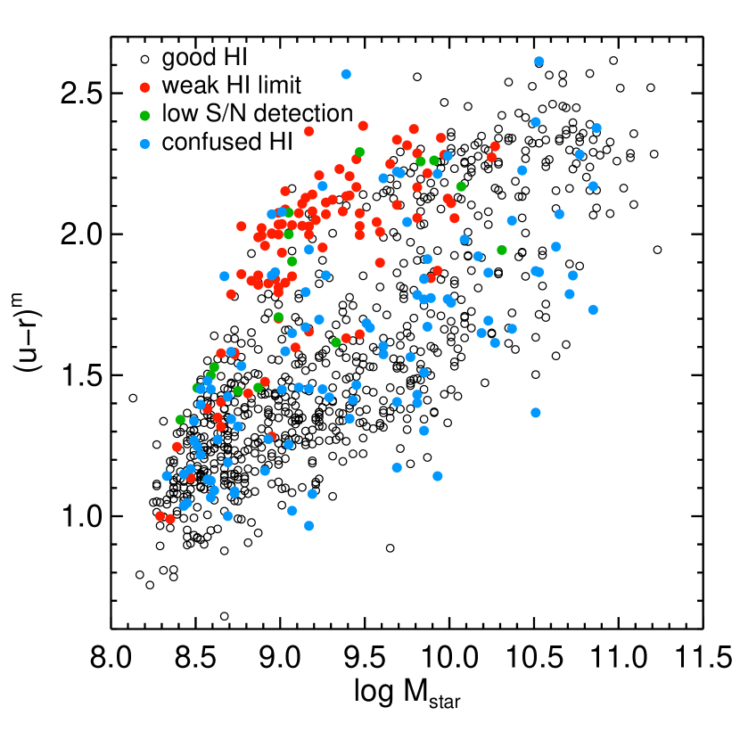
Figure 7.— Color vs. stellar mass relationship for the RESOLVE-A data set. Black open circles show galaxies with reliable HI detections as described in §3.3. Red dots show galaxies with HI upper limits yielding M_gas $>$ 0.05M_star, green dots show galaxies with low S/N detections (S/N $<$ 5), and blue dots show galaxies with HI profiles that are impossible to de-confuse. The weak upper limits tend to be the low-mass red galaxies, which are generally gas poor and have the least absolute HI content of galaxies in RESOLVE. The low S/N galaxies are also low mass, but generally bluer. The confused galaxies are interspersed throughout color and stellar mass.

4. Color-limited PGF Calibrations

In this section we describe our method to provide z=0 PGF calibrations via linear fits between log(G/S) and color. In Figure 8, we show the relationship between log(G/S) and $(u-J)^{m}$ color, which is clearly linear. However, for galaxies redder than $(u-J)^{m}$ = 3.6 mag there is a breakdown in the correlation. While the correlation between log(G/S) and $(u-J)^{m}$ color continues for some galaxies redder than 3.6 mag, we also see that the population of quenched galaxies with very low values of log(G/S) becomes more important for these same red colors. In §6, we describe a new calibration method using a 2D model fit to the probability density field of log(G/S) vs. color that allows us to model all galaxies.

Here we are generating linear fits to predict values of log(G/S) from color, where the latter has much smaller errors and thus functions as a classical independent variable. Thus, especially given the likelihood of the intrinsic scatter over and above the errors, to obtain the best predictor we should minimize residuals in log(G/S) alone (Isobe et al., 1990; Feigelson & Babu, 1992). Due to the population of red galaxies with strong HI upper limits, we must exclude all galaxies redward of a vertical color cutoff, e.g., $(u-J)^{m}$ $>$ 3.6 mag, similar to Catinella et al. (2012) and K13. Making a cut in color is appropriate for measuring the correct calibration to predict log(G/S) from color as we want to preserve the scatter for the predicted quantity (Kannappan et al., 2002) rather than fitting to only the HI detections or making a cut in log(G/S). Excluding red galaxies, however, limits the validity of our PGF calibration to galaxies blueward of the red color cutoff.

A set of such color-limited PGF calibrations for a variety of color combinations is summarized in Table 2. To create these, we use the 744 galaxies from the RESOLVE-A data set that have reliable HI detections or strong upper limits. “Reliable” HI detections are considered to include non-confused detections with S/N $>$ 5 as well as de-confused detections where the systematic error on the deconfused gas mass is $<$ 25% of the measured gas mass (see §3.3). We define strong upper limits to be those for which the gas mass is $<$ 5% of M_star. We exclude galaxies redder than the red color cutoff of each color distribution listed in Table 2 (roughly where the upper limits start to dominate). We also trim points at the blue end where the density of points is low and outliers may affect the fit as indicated in Table 2. For $(u-J)^{m}$ color, the blue color trim is 2.0 mag and the red color cutoff is 3.6 mag. Finally we perform an ordinary least squares forward fit to minimize the scatter in log(G/S), the quantity that we want to predict. We choose not to weight the fit by the measurement uncertainties in log(G/S), because they are correlated with the values of log(G/S) and color, so weighting by them would bias the fits towards galaxies with high gas content. The slope and offset in log(G/S) of these color-limited PGF calibrations are given in Table 2 along with the measured scatter in the relations and the blue color trim and red color cutoff values.

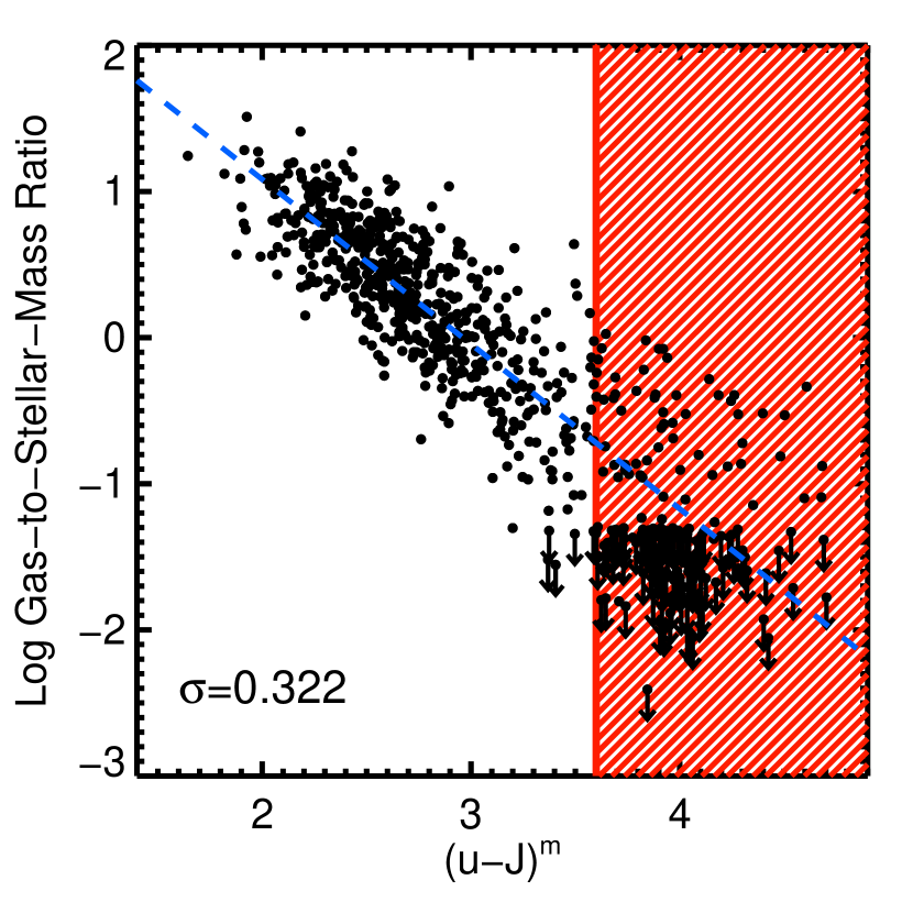
Figure 8.— Photometric gas fractions relation for $u-J$ SED modeled color, hereafter $(u-J)^{m}$. For the photometric gas fractions relation gas refers to the atomic gas content, for which we include a helium correction factor: M${}_{gas}=1.4$M_HI. When fitting, we exclude galaxies redder than $(u-J)^{m}$ = 3.6 mag, where the quenched galaxy population overwhelms the low log(G/S) end of the relationship between log(G/S) and color. We also exclude galaxies bluer than 2.0 mag as there are only a few data points that may skew the overall fit.

Table 2Color-limited Photometric Gas Fraction Calibrations

color	slope	log(G/S) offset	$\sigma$	blue trim	red cutoff	N galaxies
(mag)	(dex/mag)	(dex)	(dex)	(mag)	(mag)
$(u-r)^{m}$	-1.763	2.725	0.319	1.0	2.0	552
$(u-i)^{m}$	-1.421	2.510	0.314	1.0	2.3	571
$(u-J)^{m}$	-1.127	3.337	0.322	2.0	3.6	560
$(u-K)^{m}$	-1.059	3.993	0.331	2.8	4.4	543
$(g-r)^{m}$	-3.488	1.467	0.302	0.1	0.6	568
$(g-i)^{m}$	-2.399	1.546	0.310	0.2	0.9	557
$(g-J)^{m}$	-1.582	2.918	0.332	1.1	2.2	550
$(g-K)^{m}$	-1.401	3.744	0.364	2.0	3.0	501

We expect these fits to be useful for galaxies blueward of the blue color trim (as discussed in §7, but these calibrations do not allow us to predict gas masses for galaxies redder than the red color cutoff. We also note that color-limited linear calibrations, and all calibrations based on simple fits, are subject to bias without survival analysis to model galaxies that are confused, have weak upper limits, or lack reliable HI detections. Routines to incorporate upper limits in a linear fit exist but rely on the assumption that the upper limits are distributed randomly throughout the sample (as discussed in Isobe et al. 1986). Such “random censoring” is not the case for the PGF calibration, as those galaxies with upper limits in the RESOLVE-A data set are primarily red galaxies with low gas-to-stellar mass content. Thus using such routines would not be statistically robust. In §6 we improve on simple fitting by producing a 2D model of the log(G/S) vs. color probability density field. This fully probabilistic approach allows us to implement a version of survival analysis that reinserts the galaxies left out of the linear fits and to predict log(G/S) probability distributions for individual galaxies, even those redder than the color cutoff. Before performing this analysis, however, we analyze whether the residuals from these linear fits correlate with any other photometric parameters that may help produce tighter PGF relations.

5. Correlations with 3rd Parameters

In this section, we seek a combination of color and other photometric parameters that may produce a tighter PGF calibration for more accurate gas mass estimation. To this end we use the RESOLVE-A data set to analyze correlations between various photometric parameters and residuals from the color-limited PGF calibrations in §5.1. We then explore possible physical reasons for these residual correlations by examining their relation to galaxy morphology in §5.2. Lastly we provide plane fits between color, axial ratio, and log(G/S) for tighter color-limited PGF calibrations in §5.3.

5.1. Best 3rd Parameter for Gas Mass Estimation

Figure 9.— Measured minus predicted log(G/S) for RESOLVE-A from the PGF calibration for $(u-J)^{m}$. Residuals are plotted against a) $r$-band 50% surface brightness $\mu_{r,50}$, b) concentration index $C_{r}$ ($R_{90}/R_{e}$), c) axial ratio $b/a$, d) color gradient $\Delta_{g-r}$, e) stellar mass M_star, and f) baryonic mass M_bary. We use the Spearman Rank test to assess whether a correlation exists between the residuals in log(G/S) and these photometric parameters. The probability of no correlation and the strength of each correlation are reported for each panel. The parameters $\mu_{r50}$, $\Delta_{g-r}$, and $b/a$ have significant correlations with the residuals in log(G/S). The correlation with M_star is not physically meaningful but is caused by covariance as well as our selection on M_r,tot, a proxy for baryonic mass, which implies that the data set contains low stellar mass gas-rich objects but not low stellar mass gas-poor objects. We mark in panel e the stellar mass completeness limit for RESOLVE-A (M_bary = 9.0), below which the residuals are clearly biased towards higher log(G/S) measured than predicted. We also mark in panel f the baryonic mass completeness limit for RESOLVE-A (M_bary = 9.3). Below this limit we lack extremely gas-dominated residuals, which is expected due to the absolute magnitude limited sample, where the highest high baryonic mass-to-light ratio will fall below our M_r,tot = $-17.33$ mag limit.

As potential third parameters, we examine the surface brightness within $R_{50,r}$ ($\mu_{r,50}$), concentration index ($C_{r}$), photometric axial ratio ($b/a$), $g-r$ color gradient ($\Delta_{g-r}$), stellar mass M_star, and baryonic mass M_bary. The parameter $\mu_{r,50}$ is found by determining $R_{50,r}$ from the ellipse profiles produced in the photometric reprocessing. The $r$-band light within $R_{50,r}$ is then divided over a circular area defined by $R_{50,r}$, giving a somewhat intrinsic surface brightness for each object, although we have not applied a correction for internal galaxy extinction or optical depth since the goal is to provide a simple empirical recipe for gas estimation. Concentration index is defined as $R_{90,r}$/$R_{50,r}$ following Shimasaku et al. (2001) and Strateva et al. (2001). The $b/a$ measurement comes from the fixed ellipse fits in our photometric pipeline. $\Delta_{g-r}$ is defined as the $g-r$ color within the annulus between the $r$-band 50% and 75% light radii minus the $g-r$ color within the $r$-band half light radius, with more positive numbers meaning the galaxy has a bluer center following Kannappan et al. (2004). The stellar mass M_star is the median stellar mass from the likelihood weighted SED models described in §3.2 and the baryonic mass is M_star + M_gas.

Figure 9 shows log(G/S) residuals from the $(u-J)^{m}$ color-limited PGF calibration plotted against these different parameters. Only the data from galaxies used in the linear fit are shown, i.e., those having a color between the blue trim and red cutoff colors and reliable HI data or a strong HI upper limit. We have performed Spearman Rank tests to assess whether there is a correlation between the residuals in log(G/S) and these third parameters and quantify the strength of that correlation. Third parameters $\mu_{r,50}$, $b/a$, $\Delta_{g-r}$, and M_star all show some correlation with residuals in log(G/S), while $C_{r}$ and M_bary show no significant correlation. Below we examine each significant correlation to determine the best parameter for more accurate gas mass prediction.

The correlation between residuals in log(G/S) and M_star, shown in Figure 9e, is in the sense that low stellar mass objects tend to have higher measured log(G/S) than predicted, which is expected from covariant errors in log(G/S) and M_star. Furthermore, the bias becomes very evident for stellar mass galaxies $<$10^9.0 $M_{\odot}$ (roughly the limiting stellar mass completeness limit) marked in panel e by a dashed line. This correlation between log(G/S) residuals and stellar mass is caused by our survey selection on M_r,tot, which serves as a close proxy for baryonic mass (Kannappan & Wei, 2008, K13) rather than stellar mass. For a volume-limited, baryonic mass limited data set, an abundance of gas-rich low stellar mass objects is built in. The correlation between log(G/S) residuals and stellar mass is thus not surprising and only reflects the $r$-band magnitude selection. In Figure 9f we see that the color-limited PGF calibration does not show evidence for a correlation between residuals in log(G/S) and baryonic mass.

The remaining correlations between log(G/S) residuals and photometric parameters that we investigate are $\mu_{r,50}$, $b/a$, and $\Delta_{g-r}$. These correlations may be related to galaxy morphology and/or evolutionary state, which we explore in Figure 10 and §5.2. To decide which of these third parameters is best for use in our PGF calibrations, we use the following criteria: 1) the third parameter has a strong correlation with residuals in log(G/S), 2) the correlation between the third parameter and log(G/S) residuals is not covariant with the built in correlation between residuals in log(G/S) and stellar mass, and 3) the third parameter is a reliable, well determined quantity for all galaxies in the data set.

First we examine $\mu_{r,50}$ in Figure 9a. The correlation between residuals in log(G/S) and $\mu_{r,50}$ is such that lower surface brightness galaxies have larger log(G/S) values than predicted. The Spearman Rank test shows that the strength of the correlation between residuals in log(G/S) and $\mu_{r,50}$ is high (R = 0.43) with small probability of no correlation (P = 3$\times$10^-27). To test whether stellar mass is impacting the correlation between residuals in log(G/S) and $\mu_{r,50}$, we fit a line to the correlation between residuals in log(G/S) as a function of stellar mass, and remove the stellar mass dependence from the residuals. We then run a Spearman Rank test on the correlation between the stellar mass corrected residuals in log(G/S) and $\mu_{r,50}$, finding that the strength decreases to R = 0.28 and the probability of no correlation is larger by several orders of magnitude (P = 9$\times$10^-12) though still significant. The reliability of $\mu_{r,50}$ values is variable since $\mu_{r,50}$ is evaluated within the half light radius. For the smallest galaxies, the quantity may not truly represent the surface brightness within $R_{50,r}$.

Next we examine the third parameter $b/a$ shown in Figure 9c. The correlation between residuals in log(G/S) and $b/a$ is such that more edge-on or disky galaxies have larger log(G/S) values than predicted. The strength of the correlation between residuals in log(G/S) and $b/a$ is also high (R = $-0.39$) with small probability of no correlation (P = 3$\times$10^-22). Running a Spearman Rank test on the correlation between the stellar mass corrected residuals in log(G/S) and $b/a$, we find that both the correlation strength and the probability of no correlation remain mostly the same (R = $-0.37$ and P = 5$\times$10^-20) showing that the correlation is not affected by M_star. The $b/a$ measurements are reliable, since they are evaluated over the outer disk of the galaxy. For the smallest galaxies there may be a tendency to measure rounder objects, but since $b/a$ is evaluated in the outer disk, this issue should be minimized.

Lastly we consider the third parameter $\Delta_{g-r}$ shown in Figure 9d. The correlation between residuals in log(G/S) and $\Delta_{g-r}$ is such that galaxies with larger values of $\Delta_{g-r}$ (more blue centered) have lower log(G/S) than predicted. The strength of the correlation between residuals in log(G/S) and $\Delta_{g-r}$ is much lower than the other two parameters (R = $-0.15$) with a larger probability of no correlation (P = 5$\times$10^-4). We test whether stellar mass is impacting this correlation between residuals in log(G/S) and $\Delta_{g-r}$, by removing the correlation between residuals in log(G/S) and stellar mass. Running a Spearman Rank test on the correlation between the stellar mass corrected residuals in log(G/S) and $\Delta_{g-r}$, we find that both the correlation strength becomes stronger (R = $-0.25$) and the probability of no correlation becomes several orders of magnitude smaller (P = 8$\times$10^-10). The correlation between $\Delta_{g-r}$ and stellar mass has been shown previously in Stark et al. (2013) and it is apparent that the stellar mass affects how this third parameter relates to residuals in log(G/S). The reliability of the measurement may be suspect for the smallest galaxies, since it requires measuring colors within $R_{50,r}$ and between $R_{50,r}$ and $R_{75,r}$.

The quantity that best meets our three criteria is $b/a$ since it exhibits a strong correlation with the residuals in log(G/S) that is not affected by the correlation with stellar mass. The measurement of $b/a$ is also the least likely to be affected by systematics from the photometry, including the convolution of galaxy SDSS and UKIDSS images to a common psf since it is a measure of the axial ratio in the outer disk.

5.2. Physical Drivers of Residual Correlations

For the purpose of defining PGF calibrations, we do not strictly need to understand the drivers of the correlations, but we explore them briefly here, deferring a more thorough discussion to future work. To aid our interpretation, we analyze log(G/S) residuals as a function of the best third parameter options and galaxy morphology in Figure 10. Morphologies come from visual classification for the RESOLVE data set (Moffett et al., submitted, Kannappan et al. in prep.). Since galaxy morphology is generally not available for large data sets and can be subjective and unreliable especially for small and edge-on galaxies, we have not used morphology for the general analysis of third parameters for improved gas mass estimation. In Figure 10 we plot galaxy morphology vs. $\mu_{r,50}$, $b/a$, and $\Delta_{g-r}$ and color code the residuals in log(G/S) such that green represents galaxies for which the PGF calibration underpredicts values of log(G/S), yellow represents galaxies for which the PGF calibration predicts values of log(G/S) similar to the measured values, and red represents galaxies for which the PGF calibration overpredicts values of log(G/S).

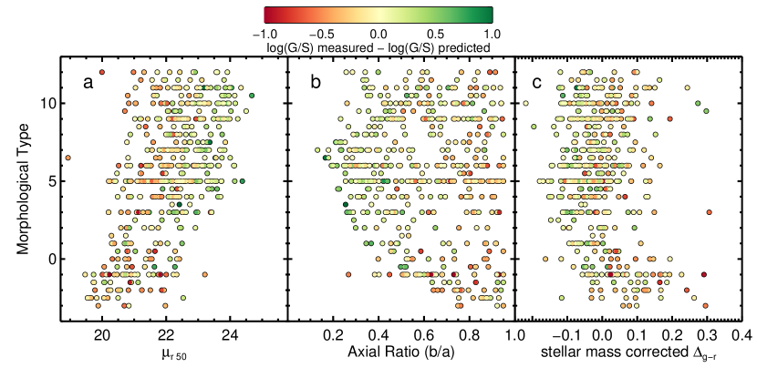
Figure 10.— Residuals in log(G/S) (dot color) shown within plots of galaxy morphological type vs. (a) $\mu_{r,50}$, (b) $b/a$, and (c) stellar mass corrected $\Delta_{g-r}$ (following Stark et al., 2013). The color scale is shown at the top, where green marks galaxies for which the PGF calibration underpredicts values of log(G/S), yellow marks galaxies for which the PGF calibration values of log(G/S) similar to the measured values, and red marks galaxies for which the PGF calibration overpredicts values of log(G/S). Late-type galaxies (T $>$ 0) with underpredicted values of log(G/S) tend to be lower surface brightness, more edge-on, and have redder centers (smaller values of stellar mass corrected $\Delta_{g-r}$). These trends become somewhat less noticeable for dwarf types (T $>$ 8), and in general for early-type galaxies values of log(G/S) tend to be overpredicted (with the caveat that most red-sequence early-types are redder than our red color cut so not shown). We discuss the physical significance of these patterns in §5.2.

First we examine the relationship between morphological type and $\mu_{r,50}$ in Figure 10a. It appears that among late-type galaxies (T$>$0), the PGF calibration overpredicts values of log(G/S) for those galaxies with $\mu_{r,50}$ brighter than 22 and underpredicts log(G/S) for those galaxies with $\mu_{r,50}$ fainter than 22. For early-type galaxies, which mostly have $\mu_{r,50}$ brighter than 22, we generally overpredict log(G/S). The transition around $\mu_{r,50}$ $\sim$ 22 seems to indicate that even for a specific type of galaxy, those galaxies that are lower surface brightness are on average more gas-rich than their higher surface brightness counterparts. Gas richness has long been associated with low surface brightness galaxies (e.g.,de Blok et al., 1996 and O’Neil et al., 2004), and we show this result for a statistical population of galaxies using RESOLVE-A.

Next we examine the relationship between morphological type and $b/a$ in Figure 10b. Within the population of late-type spirals (0 $<$ T $<$ 8), edge-on spirals tend to have underpredicted values of log(G/S). This phenomenon makes sense for larger edge-on spirals, which are observed to be redder than their intrinsic colors due to dust extinction (e.g., Conroy et al., 2010 show that for star forming galaxies over the narrow stellar mass range 9.5 $<$ log M_star $<$ 10, those with $b/a$ $\sim$ 0.35 are redder than those with $b/a$ $\sim$ 0.95). Thus the underprediction may result because these edge-on late type spirals are shifted redward of their true color measurement, where the typical value of log(G/S) is smaller. The trend towards underpredicting edge-on galaxy values is less noticeable for edge-on irregular dwarf-type galaxies (T $>$ 8) that are likely pure disk, low surface brightness galaxies with little internal extinction due to dust (e.g., Dalcanton et al., 2004). For early-type galaxies, we see that in general values of log(G/S) are overpredicted with no obvious trend with $b/a$.

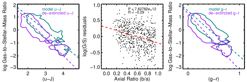
Figure 11.— Test of the effect of dust on the relationships between log(G/S), color, and axial ratio. a) Log(G/S) vs. $u-J$ color comparing the model (green) vs. de-extincted (purple) colors. Contours are shown encompassing 90% of all galaxies excluding confused galaxies and weak upper limits. Dashed lines show the color-limited linear fits to the data. The relationship steepens when using the de-extincted colors. b) Versus $b/a$, the residuals in log(G/S) from the de-extincted $u-J$ PGF calibration have a smaller strength of correlation and significance than the residuals computed from the model $u-J$ PGF calibration, but the correlation is still highly significant (the red-dashed line shows the linear fit). c) Same as panel a except using $g-r$ color (as in Jaskot et al., 2015). Unlike Jaskot et al. (2015) we do not find that the relationship between log(G/S) and $g-r$ disappears completely when using de-extincted colors, although we do see that the relationship steepens, meaning dust is a contributing factor to the relationship.

We show the PGF calibrations using both model (green) and de-extincted (purple) $u-J$ colors in Figure 11a (we also show the PGF calibrations using $g-r$ color in Figure 11c). The relationship between log(G/S) and color becomes steeper (less predictive) when using the de-extincted rather than model colors (Figure 11a/c), similar to the result shown in Jaskot et al. (2015). We do not find, however, that that the PGF correlation completely disappears when using de-extincted colors, suggesting that while dust plays a role in the PGF calibration, long-term star formation is also important (K13). We suspect that star formation history is in fact related to dust extinction, which we plan to follow up in future work. In Figure 11b we show the residuals in log(G/S) from the de-extincted PGF correlation as a function of axial ratio, and we find that the strength and significance of the third parameter correlation are smaller but still highly significant. Additional effects, perhaps related to the morphology-surface brightness correlation, may also be important.

Nevertheless, as the goal of this work is to provide empirical PGF calibrations for predicting gas masses, we prefer not to correct for extinction, since uncorrected colors provide the best (most linear and most predictive) calibrations. Moreover, uncorrected colors are not as dependent on modeling.

Lastly we examine the relationship between morphological type and stellar mass corrected $\Delta_{g-r}$ in Figure 10c. We correct $\Delta_{g-r}$ values for the correlation between $\Delta_{g-r}$ and stellar mass as in Stark et al. (2013) to show the effects more strongly. Late-type galaxies are generally more red-centered with a slight trend towards bluer centers for later types (larger values of T), while early-type galaxies tend to be more blue centered as most of these are blue-sequence E/S0s (Kannappan et al., 2009) because normal red-sequence E/S0s are excluded by our color cut.

Within the late-type population, for a given morphological type more blue centered galaxies have overpredicted values of log(G/S). This result is intriguing because among late-type galaxies, blue centered galaxies are associated with recent star formation events due to interactions (Kannappan et al., 2004), and have higher M${}_{H_{2}}$/M_HI ratios and lower M_HI/M_star ratios (Stark et al., 2013). Including the molecular gas for such blue-centered late-type galaxies that are offset low in the color-limited PGF calibration may bring their total gas-to-stellar mass ratio (where total gas mass = 1.4M_HI + M${}_{H_{2}}$) in line with the general relationship between log(G/S) and color as shown in Figure 8 of K13.

The analysis of log(G/S) residuals as a function of galaxy morphology and the aforementioned three photometric parameters reveals physical trends for all three that may have implications for galaxy evolution. The two parameters $\mu_{r,50}$ and $\Delta_{g-r}$, however, are both covariant with stellar mass, so their ability to reduce scatter is partially artificial. Using $b/a$ allows us to minimize scatter in a physically meaningful way without introducing covariance into the PGF calibration.

5.3. Modified Color-Limited PGF Calibration

To use $b/a$ in PGF calibrations, we compute a linear combination of color and $b/a$ to be the new predictor. We call this combination of color and $b/a$ “modified color.” First, we fit a plane in color, $b/a$, and log(G/S), minimizing scatter in log(G/S) and only using those data points that fall within the blue color trim and red color cutoff for a particular color choice. The planar fit determines coefficients such that modified color = $m_{0}$$\times$color + $m_{1}$$\times$($b/a$).

We then use the relationship between modified color and log(G/S) to create tighter modified color-limited PGF calibrations. We use the same procedure as in §4. First we limit our data set to the 744 galaxies with reliable HI data. Then we define a red modified color cutoff and a blue modified color trim just as in §4. Lastly we perform an ordinary least squares forward fit. Again we choose not to weight the fit by the errors on log(G/S) due to correlations between the uncertainties and both galaxy color and log(G/S) itself. Table 3 gives the modified color coefficients $m_{0}$ and $m_{1}$, the slope of the linear fit, the offset in log(G/S), and the $\sigma$ of the modified color PGF calibrations. The blue modified color trim and red modified color cutoff are also given as well as the number of galaxies used in each modified color fit. We note that the scatter for the PGF calibrations using modified colors based on $u$ and $g$ are typically reduced by $\sim$0.03 dex as compared to the PGF calibrations using color only. Another advantage of using the modified color calibrations is the generally increased baseline (or range) of the predictor value.

We note that many other works have used planes defined by color and other galaxy structural parameters to define tighter PGF calibrations (Zhang et al., 2009; Catinella et al., 2010; Li et al., 2012; Catinella et al., 2013), often choosing stellar mass surface density or surface brightness, which reduce scatter partially due to covariance with log(G/S). In Catinella et al. (2013), the authors use the term “gas fraction planes” to refer to these PGF calibrations. We choose to use the terminology “modified color” to refer specifically to the predicting quantity, which is a linear combination of color and a structural parameter, in this work chosen to be $b/a$.

Table 3Modified Color-limited Photometric Gas Fraction Calibrations

modified color	slope	log(G/S) offset	$\sigma$	blue trim	red cutoff	N galaxies
(mag)	(dex/mag)	(dex)	(dex)	(mag)	(mag)
1.822$(u-r)^{m}$ + 0.609($b/a$)	-0.958	3.038	0.296	2.0	4.1	580
1.454$(u-i)^{m}$ + 0.595($b/a$)	-0.989	2.887	0.291	1.8	3.8	579
1.140$(u-J)^{m}$ + 0.594($b/a$)	-0.981	3.659	0.304	2.5	4.5	581
1.075$(u-K)^{m}$ + 0.605($b/a$)	-0.952	4.228	0.302	3.3	5.0	525
3.563$(g-r)^{m}$ + 0.534($b/a$)	-1.002	1.813	0.281	0.7	2.6	582
2.444$(g-i)^{m}$ + 0.550($b/a$)	-0.984	1.881	0.287	0.8	2.6	568
1.592$(g-J)^{m}$ + 0.550($b/a$)	-0.980	3.218	0.313	2.1	3.8	540
1.435$(g-K)^{m}$ + 0.618($b/a$)	-0.864	3.678	0.306	2.8	4.5	488

6. Probability Density Field PGF Calibrations

Due to the limitations of the color-limited linear fits, we present in this section a new PGF calibration method that improves over the color-limited fits in three ways. First, the new method provides a full probability distribution in log(G/S) for each galaxy given its color or modified color rather than a single number for log(G/S). Second, we are able to model the galaxy distribution past the red color cutoff region where quenched galaxies coexist with star-forming galaxies. Third, in the spirit of survival analysis, we develop a Monte Carlo method to reinsert the 22% of RESOLVE-A galaxies with unreliable HI data in the calibration, thus determining the calibration for the entire volume-limited data set. We describe the full probability distribution method in §6.1, and we outline the Monte Carlo method to reinsert unreliable galaxies in §6.2. Instructions on how to use the calibration are provided in §6.3. Lastly in §6.4, we examine whether the model changes significantly if we add in the small subset of galaxies that have M_r,tot fainter than $-17.33$, but still have M_bary $>$ 10^9.3 $M_{\odot}$. For simplicity, throughout these sections we use the variable “$mc$” to refer to either color alone or modified color that includes a $b/a$ term.

6.1. Calibration Description

To start we use the same RESOLVE-A galaxies as in §4, those with reliable detections or strong upper limits. Detections are considered reliable if they are not confused or are deconfused with systematic errors $<$ 25% of the HI mass measurement and have S/N $>$ 5. Limits are considered strong if they provide a gas mass measurement of M_gas $<$ 0.05M_star. We show log(G/S) vs. modified $(u-J)^{m}$ color for the RESOLVE-A data set limited to reliable gas data in Figure 12a. This definition excludes 211 galaxies (of 955 total) in RESOLVE-A, however we describe how a technique based on survival analysis principles to include these galaxies in the PGF calibration in §6.2.

For galaxies with upper limits, we cannot know the value of the HI mass, only that it is less than a certain value. We choose to set all galaxies, both detections and limits, with log(G/S) $<$ $-1.3$ to log(G/S) = $-1.3$, which is 5% of the stellar mass in linear units. This choice is fine for measuring a galaxy’s baryonic mass (as in the companion paper Eckert et al. in prep.), because a galaxy’s baryonic mass will not be significantly affected if it is at most 1.05M_star. In Figure 12a, we demonstrate the data replacement with red arrows.

Next we determine the density field of galaxies in log(G/S) vs. $mc$ by binning in both dimensions and measuring the number of galaxies in each 2D bin or cell of log(G/S) and $mc$. The density field is shown in Figure 12b. We use bin sizes of 0.2 dex in log(G/S) and 0.2 mag in $(u-J)^{m}$. When determining the bin size for each $mc$, we start with bin sizes of 0.2 mag and require a minimum of 10 bins in color to ensure adequate sampling of the calibration. If there are less than 10 bins (as is the case for colors with small ranges such as $g-r$) we switch to bin sizes of 0.1 mag.

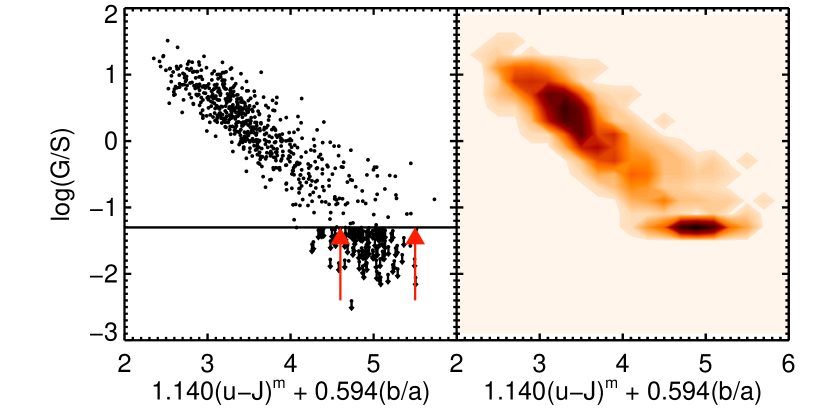
Figure 12.— Log(G/S) vs. modified $(u-J)^{m}$ color for RESOLVE-A. The modified color is the linear combination of $(u-J)^{m}$ and $b/a$ that produces the best plane fit with log(G/S) as described in §5.3. a) Scatter plot showing reliable HI detections with small black dots, and strong upper limits with downward black arrows. Galaxies with log(G/S) values $<$ $-1.3$ (marked by the black line), whether they are detections or limits, are replaced with $-1.3$ (as indicated by the red arrows). b) Contour plot showing the PGF density field of log(G/S) vs. modified $(u-J)^{m}$ color, where each cell’s value is the number of galaxies in that cell. The contours are spaced finely over 100 intervals between 0 and 34 (the maximum number of galaxies found in a cell). We fit the model described in §6.1 to this PGF density field.

To model the PGF probability density field we assume two distinct populations: detections and upper limits. The detections lie on a line with Gaussian scatter that widens towards redder colors. The limits appear only at red $mc$ and are confined to a value of log(G/S) = $-1.3$ although they may in fact have much lower values. The model consists of nine parameters given by $A_{0}$ to $A_{8}$.

To model the population of detections we first model the peak value of the Gaussian at each $mc$, designated as $\rho_{0}$, as a log-normal function of $mc$ as given in equation 1. $A_{0}$ provides the normalization, $A_{1}$ is the location parameter in $mc$, and $A_{2}$ is the shape parameter.

$$\rho_{0}=\frac{A_{0}}{(mcA_{2}\sqrt{2\pi})}\times\exp(\frac{-(\ln(mc)-A_{1})^{2}}{2A_{2}^{2}})$$ (1)

The number density of detections ($D$) is then described by a Gaussian with peak value $\rho_{0}$ that changes with $mc$, with mean log(G/S) value ($A_{3}mc+A_{4}$) that decreases linearly for larger values of $mc$, and with standard deviation $A_{5}mc$ that widens towards larger values of $mc$. The model for the detections is given in equation 2.

$$D=\rho_{0}\times\exp(\frac{-(log(G/S)-(A_{3}mc+A_{4}))^{2}}{2(A_{5}mc)^{2}})$$ (2)

At red $mc$, there are galaxies with values of log(G/S) $<$ $-1.3$ that belong to the detection rather than limit population. Because we have chosen to set all galaxies with values of log(G/S) $<$ $-1.3$ to be equal to $-1.3$, we must divide up equation 2 to account for the tail of the detection population with log(G/S) $<$ $-1.3$. For values of log(G/S) $>$ $-1.3$, the model is as given by equation 2, but for values of log(G/S) = $-1.3$, we model the detection population by integrating the tail of the Gaussian at a given $mc$ over all log(G/S) $<$ $-1.3$. Thus the detection population for log(G/S) $<$ $-1.3$ is given in equation 3.

$$D=\rho_{0}\frac{1}{2}A_{5}mc\sqrt{2\pi}\times[1-erf(\frac{\left|-1.3-(A_{3}mc+A_{4})\right|}{\sqrt{2(A_{5}mc)^{2}}})]$$ (3)

The upper limit population is evaluated only at log(G/S) $=$ $-1.3$ and is modeled as a Gaussian function of $mc$ with a peak value $A_{6}$, color shift $A_{7}$, and standard deviation $A_{8}$ as given in equation 4. The Gaussian shape captures the fact that blue galaxies rarely have low gas fractions and on the other side that there is a natural decline in galaxies towards redder colors.

$$L=A_{6}\times\exp(\frac{-(mc-A_{7})^{2}}{2A_{8}^{2}})$$ (4)

The full-probability PGF model is the combination of equations 2, 3, and 4, and we fit this model to the PGF density field using the MPFIT2DFUN package (Markwardt, 2009), which performs a Levenberg-Marquardt least squares fit (Moré, 1978). We weight each cell value in the density field, which is the number of galaxies in the cell N, by 1/N. From the fit we obtain the parameters $A_{0}$ through $A_{8}$ that best describe the PGF calibration. We recognize that the probability density field model is more complex than a simple linear fit. However, the advantages of being able to fit both the detection and limit populations and of being able to reinsert the data from galaxies without adequate HI data (see §6.2) make it a more powerful technique for estimating gas masses (see §7).

6.2. Reinserting the Missing Galaxies

To measure probability density field PGF calibrations with the complete RESOLVE-A data set, we implement a custom version of survival analysis following its basic algorithm: create a model of the missing/censored data points based closely on the available data and sample it with Monte Carlo methods. The model for each censored/missing data point is determined from the uncensored data in an initial fitting round as in traditional survival analysis, with the restriction that limits must be drawn from a model distribution truncated at the limit values. We then iterate this procedure a second time using the updated model resulting from the first round. The steps are as follows.

1) After performing the initial PGF model fit from §6.1 using only the reliable HI data in RESOLVE-A, we obtain a PGF model with initial best fit parameters $A_{i,0}$ through $A_{i,8}$. Using these initial best fit parameters, we obtain a probability distribution in log(G/S) for each galaxy with unreliable HI data given its $mc$. For galaxies with weak upper limits, we restrict the probability distributions in log(G/S) to only those values below the upper limit, then we renormalize the probability distribution. For low S/N detections and confused galaxies we do not place any restrictions on the probability distribution in log(G/S).

2) We then randomly assign a value of log(G/S) for each of these 211 galaxies from each respective probability distribution using the inverse transform sampling method.

3) Next, we create a new PGF density field that includes both the 744 data points with reliable HI and the 211 data points with randomly assigned values of log(G/S) from their respective probability distributions. We fit the PGF calibration model as described in §6.1 and save the best fit parameters $A_{n,0}$ through $A_{n,8}$. We also compute residuals for each best fit model as well as the reduced $\chi^{2}$ goodness of fit, assuming the variance on the data value for each cell is $\sigma^{2}$ = N (the number of galaxies in the cell).

4) We perform steps 2 & 3 100 times and save the best fit parameters and reduced $\chi^{2}$ values for each round. We then calculate the median values of the parameters based on those 100 rounds $A_{med,0}$ through $A_{med,8}$, which describe the new model for the PGF density field. We save the median reduced $\chi^{2}$ as well.

5) We iterate once more through steps 1-4 using the model parameters $A_{med,0}$ through $A_{med,8}$ to produce the initial probability distributions in log(G/S) for the 211 galaxies with unreliable HI data. This iteration allows us to determine log(G/S) probability distributions based on the PGF density field calibrated with all RESOLVE-A galaxies, not just those with reliable HI data. After this second iteration, we take the values of $A_{med,0}$ through $A_{med,8}$ to be the final best fit parameters $A_{f,0}$ through $A_{f,8}$ for the full-probability PGF model. We have tested whether more iterations are necessary, however after the second iteration the values of $A_{med,0}$ through $A_{med,8}$ change very little ($<$ 3% of the final value). The final values do change significantly from the initial fit (which includes only the reliable HI galaxies), with final values up to $\sim$20% different from the initial values.

Figure 13 shows a contour plot of the best fit model and residuals using modified $(u-J)^{m}$ color, where the residuals have been normalized by the number of galaxies in each cell. The 211 galaxies with unreliable HI data have been assigned values of log(G/S) pulled at random from their respective distributions in log(G/S), as in step 2, using the final best fit parameters. The residuals are most significant for the highest log(G/S) cells at red modified color where there are few galaxies (often just one per cell).

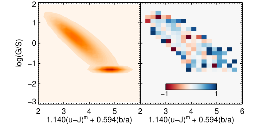
Figure 13.— Best fit model to the PGF density field using modified $(u-J)^{m}$ color. a) The best fit model is shown as a contour plot (as for Figure 12b divided into 100 levels between 0 and 44, the maximum number of galaxies found in a cell after reinsertion of galaxies with inadequate HI data). b) Residuals for each cell normalized by the number of galaxies in each cell so the range is from $-1$ to 1. Overall the model performs well, although there are large residuals especially around the edges of the calibration where the number density of galaxies is low.

6.3. How to Use the PGF Calibration

The parameters in Tables 4 and 5 provide the best fit models to the PGF density field probability distribution, which is not normalized at a given value of $mc$. To create conditional probability distributions in log(G/S) at each $mc$, the PGF distribution for a given $mc$ from equations 2, 3, and 4 should be divided by the integral of the PGF at that $mc$. Examples of such distributions are shown in Figure 14 for modified $(u-J)^{m}$ color $mc$ = 3.1 (blue), 4.4 (green), and 5.3 (red). We note that the sharp spike in the log(G/S) probability distribution is entirely due to the way in which upper limits and low gas-fraction galaxies are treated in the model and should not be interpreted literally as probability distributions for this population.

Table 4Full-Probability Photometric Gas Fractions Calibrations for Color Only

color	$A_{f,0}$	$A_{f,1}$	$A_{f,2}$	$A_{f,3}$	$A_{f,4}$	$A_{f,5}$	$A_{f,6}$	$A_{f,7}$	$A_{f,8}$	reduced $\chi^{2}$
(mag)
$(u-r)^{m}$	17.22	0.33	0.22	-1.67	2.56	0.21	47.65	2.21	0.14	1.353
$(u-i)^{m}$	35.05	0.46	0.24	-1.37	2.40	0.19	68.44	2.55	0.20	1.518
$(u-J)^{m}$	32.55	1.00	0.17	-1.04	3.07	0.11	53.39	3.88	0.26	1.257
$(u-K)^{m}$	30.18	1.26	0.13	-0.99	3.75	0.09	42.35	4.79	0.33	1.422
$(g-r)^{m}$	19.70	-1.15	0.48	-3.65	1.51	0.87	115.1	0.72	0.05	1.831
$(g-i)^{m}$	19.99	-0.70	0.45	-2.47	1.58	0.55	72.29	1.05	0.09	1.344
$(g-J)^{m}$	16.99	0.51	0.19	-1.52	2.80	0.18	42.87	2.37	0.16	1.036
$(g-K)^{m}$	31.08	0.91	0.15	-1.22	3.27	0.14	61.95	3.29	0.22	1.246

Table 5Full-Probability Photometric Gas Fractions Calibrations for Modified Color

modified color	$A_{f,0}$	$A_{f,1}$	$A_{f,2}$	$A_{f,3}$	$A_{f,4}$	$A_{f,5}$	$A_{f,6}$	$A_{f,7}$	$A_{f,8}$	reduced $\chi^{2}$
(mag)
1.822$(u-r)^{m}$ + 0.609(b/a)	38.78	1.05	0.20	-0.89	2.80	0.09	47.95	4.44	0.29	1.125
1.454$(u-i)^{m}$ + 0.595(b/a)	37.78	0.97	0.21	-0.93	2.70	0.10	51.88	4.10	0.27	1.104
1.140$(u-J)^{m}$ + 0.594(b/a)	38.13	1.25	0.16	-0.93	3.49	0.08	44.57	4.82	0.31	1.066
1.075$(u-K)^{m}$ + 0.605(b/a)	34.54	1.43	0.14	-0.88	3.92	0.07	40.53	5.53	0.34	1.157
3.563$(g-r)^{m}$ + 0.534(b/a)	42.65	0.37	0.37	-0.97	1.74	0.18	62.12	2.92	0.21	1.166
2.444$(g-i)^{m}$ + 0.550(b/a)	40.95	0.45	0.36	-0.99	1.87	0.17	60.79	2.95	0.21	1.228
1.592$(g-J)^{m}$ + 0.550(b/a)	36.40	1.10	0.18	-0.94	3.08	0.10	51.50	4.16	0.26	1.028
1.435$(g-K)^{m}$ + 0.618(b/a)	33.79	1.37	0.14	-0.91	3.83	0.08	45.48	5.10	0.31	1.182

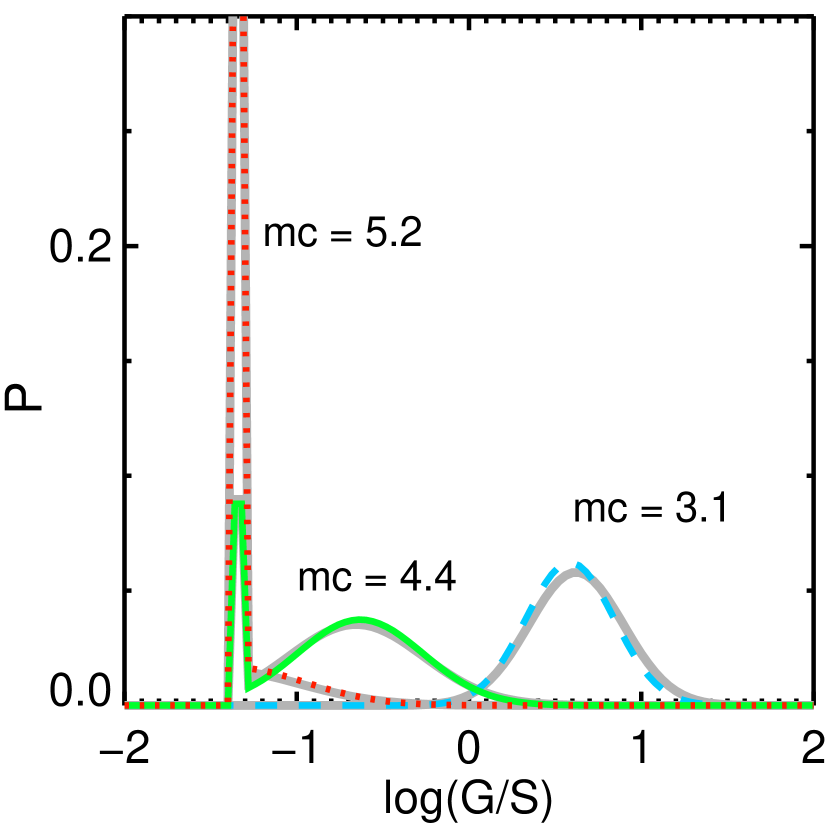
Figure 14.— Probability distributions for three galaxies with modified $u-J$^m “$mc$” = 3.1, 4.4, and 5.2, which are labeled on the plot. For blue modified colors the distribution in log(G/S) is Gaussian ($mc$ = 3.1). The $\sigma$ value of the Gaussian widens for redder modified colors ($mc$ = 4.4), where the population of galaxies with log(G/S) $<$ $-1.3$ also increases. The sharp spike at log(G/S) = $-1.3$ is due to the way in which galaxies with upper limits or low gas-fractions are treated in the model. For the reddest colors ($mc$ = 5.2)the contribution from the upper limit population with log(G/S) $<$ $-1.3$ becomes dominant. In solid grey we show the probability distributions for the same modified colors when using the fits that include high baryonic mass-to-light galaxies as explained in 6.4. The largest difference occurs for the bluest galaxy, although the difference is quite small.

6.4. Adding in High M_bary/L Galaxies

As a check, we have also performed the full-probability PGF calibration using a slightly altered RESOLVE-A data set. This data set aligns with the spectroscopic observing data set for the RESOLVE survey. We consider all galaxies with M_r,tot brighter than $-17.33$ as well as any galaxies with M_bary $>$ 10^9.3 $M_{\odot}$ no matter their M_r,tot, thus including the highest baryonic mass-to-light ratios that fall out of the absolute magnitude limited sample.

For this test we use the PGF calibrations from Tables 4 and 5 to estimate gas masses for the galaxies with M_r,tot fainter than $-17.33$ that do not have adequate gas data. Using the median value of log(G/S) from each probability distribution we estimate the gas mass for these galaxies. We then compute M_bary for each galaxy in the RESOLVE-A region, adding the stellar mass to either the measured M_gas for those galaxies with reliable detections and strong upper limits, or the predicted M_gas for those galaxies with low S/N detections, confused profiles, or weak upper limits. Adding galaxies with M_r,tot fainter than $-17.33$ and M_bary $>$ 10^9.3 $M_{\odot}$ yields a RESOLVE-A data set with 39-40 additional galaxies depending on the choice of PGF calibration. Thirty-nine of those galaxies have reliable HI data.

With these galaxies added, we can now run through the same procedure as detailed in §6.1 and §6.2. The parameters for the best fit models are given in Tables 6 and 7. The PGF calibrations yield similar log(G/S) distributions with or without the high baryonic mass-to-light ratio galaxies. In Figure 14 grey solid lines show the log(G/S) probability distributions for $mc$ = 3.1, 4.4, and 5.2 when including the high baryonic mass-to-light ratio galaxies. The largest difference is seen for the bluest galaxies, where the high baryonic-mass-to-light galaxies very slightly shift the probability distribution towards higher values of log(G/S).

Table 6Full-Probability Photometric Gas Fractions Calibrations for Color Only Including High M_bary/L Galaxies

color	$A_{f,0}$	$A_{f,1}$	$A_{f,2}$	$A_{f,3}$	$A_{f,4}$	$A_{f,5}$	$A_{f,6}$	$A_{f,7}$	$A_{f,8}$	reduced $\chi^{2}$
(mag)
$(u-r)^{m}$	34.56	0.31	0.23	-1.66	2.57	0.24	90.35	2.21	0.15	1.514
$(u-i)^{m}$	35.01	0.44	0.24	-1.44	2.54	0.20	68.48	2.55	0.20	1.474
$(u-J)^{m}$	32.37	1.00	0.17	-1.10	3.28	0.12	53.83	3.88	0.26	1.308
$(u-K)^{m}$	29.47	1.26	0.13	-1.03	3.93	0.10	42.53	4.78	0.33	1.446
$(g-r)^{m}$	19.24	-1.17	0.49	-3.74	1.56	0.93	115.8	0.72	0.05	2.033
$(g-i)^{m}$	19.75	-0.71	0.45	-2.54	1.63	0.58	72.31	1.05	0.09	1.514
$(g-J)^{m}$	32.44	0.50	0.20	-1.54	2.87	0.22	82.06	2.39	0.17	1.098
$(g-K)^{m}$	29.46	0.91	0.15	-1.29	3.46	0.15	62.12	3.29	0.23	1.323

Table 7Full-Probability Photometric Gas Fractions Calibrations for Modified Color Including High M_bary/L Galaxies

modified color	$A_{f,0}$	$A_{f,1}$	$A_{f,2}$	$A_{f,3}$	$A_{f,4}$	$A_{f,5}$	$A_{f,6}$	$A_{f,7}$	$A_{f,8}$	reduced $\chi^{2}$
(mag)
1.822$(u-r)^{m}$ + 0.609(b/a)	38.82	1.05	0.21	-0.90	2.84	0.10	48.06	4.44	0.29	1.194
1.454$(u-i)^{m}$ + 0.595(b/a)	37.44	0.96	0.21	-0.96	2.79	0.11	51.32	4.10	0.27	1.188
1.140$(u-J)^{m}$ + 0.594(b/a)	36.98	1.24	0.16	-0.98	3.66	0.08	44.90	4.82	0.31	1.154
1.075$(u-K)^{m}$ + 0.605(b/a)	33.11	1.43	0.14	-0.91	4.05	0.07	40.99	5.53	0.34	1.219
3.563$(g-r)^{m}$ + 0.534(b/a)	41.40	0.36	0.37	-1.01	1.82	0.19	61.93	2.91	0.21	1.299
2.444$(g-i)^{m}$ + 0.550(b/a)	39.53	0.44	0.35	-1.03	1.97	0.18	60.35	2.95	0.21	1.309
1.592$(g-J)^{m}$ + 0.550(b/a)	35.19	1.10	0.18	-0.97	3.20	0.10	51.74	4.16	0.26	1.171
1.435$(g-K)^{m}$ + 0.618(b/a)	32.02	1.37	0.14	-0.94	3.96	0.08	45.97	5.10	0.31	1.216

7. Discussion

In this section we perform two comparisons of PGF calibrations from this work and other work using the RESOLVE-B data set. First, we compare predicted gas masses from PGF calibrations with measured gas masses from the RESOLVE-B data set as a function of stellar mass. To test the different PGF calibrations, we select only galaxies in RESOLVE-B that have reliable HI detections (294 out of 487), as upper limits are not ideal candidates for this test. Second, we compare the actual RESOLVE-B distribution of log(G/S) in bins of $(u-J)^{m}$ color with the predicted distributions of log(G/S) based on these different calibrations.

To test the probability density field model we use the modified $(u-J)^{m}$ color calibration (top row of Figure 15). Since the calibration provides a probability distribution of log(G/S) for each galaxy, we use the median value from the probability distribution in log(G/S) for the purposes of the first test. In the top panel of Figure 15 we find that using the probability density field model PGF calibration yields a negligible offset and small scatter = 0.343 dex. For the lowest stellar masses, we see asymmetric scatter towards larger measured than predicted gas masses. As indicated by the arrow in the bottom panel of Figure 15, this asymmetric scatter is consistent with covariance between stellar mass, plotted on the x-axis, and the predicted gas mass in the denominator of the y-axis (note that estimated G/S is multiplied by stellar mass to obtain gas masses). We also show the distribution of log(G/S) predicted for RESOLVE-B galaxies in four bins of $(u-J)^{m}$ color, drawing a random value from the log(G/S) distribution of each RESOLVE-B galaxy. The probability density field model works well across all colors.

To test our color-limited linear fits, we use the calibration based on $(u-J)^{m}$ color. While the $(u-J)^{m}$ calibration has higher scatter than calibrations based on optical colors, the $(u-J)^{m}$ calibration has a larger predictive range as compared to typical errors on color (considering the slopes that would multiply the error; see Tables 2 and 3. In the second row of Figure 15, we show the log of the measured gas mass divided by the predicted gas mass as a function of stellar mass. We find a negligible offset between the measured and predicted gas mass measurements and a scatter of $\sigma$ = 0.361 dex, slightly higher than found in the color-limited PGF calibration itself and slightly higher than the probability density field model. We next show the log(G/S) distributions predicted for RESOLVE-B with the color-limited linear fit, where we add random scatter with $\sigma$ = 0.31 dex to log(G/S) estimates. The second test reveals the weakness of the color-limited approach as it cannot reproduce the distribution of log(G/S) for red galaxies in RESOLVE-B.

In the third row, we test the calibration based on the NFGS given in K13, log(G/S) = $-0.98$$(u-J)^{m}$ + 2.70. The NFGS has been run through the same photometric pipeline and stellar population modeling code as for this work, so we are able to use the same SED modeled colors and stellar mass estimates to predict gas masses. There is a significant offset (0.172 dex) towards underpredicting gas mass measurements, with that offset increasing for low stellar mass galaxies. The same issue can be seen in the second test, where the K13 calibration systematically underestimates the distribution of log(G/S) for blue galaxies and overestimates the distribution of log(G/S) for red galaxies in RESOLVE-B.

A similar problem is seen for the color-limited (NUV$-r$ $<$ 4.5) PGF calibration based on GASS from Catinella et al. (2013), log(G/S) =$-0.234$log($\mu_{*}$)$-0.342$(NUV$-r$) + 2.329. This color-limited calibration attempts to reduce residuals for gas-rich galaxies. We note that the GASS survey calibration does not take into account a helium correction factor so we multiply the gas mass value obtained from this calibration by 1.4 to compare with the gas mass measurements in RESOLVE-B. To match their parameters we use NUV$-r$ total colors measured for the RESOLVE survey, which are similar to the Kron NUV$-r$ colors measured for the GASS survey, although subject to differences in the optical sky background subtraction and magnitude extrapolation. GASS defines $\mu_{*}$ = $M_{*}$/(2$\pi$$R^{2}_{50,z}$), where $R^{2}_{50,z}$ is the $z$-band Petrosian half-light radius in kpc. We use the stellar mass measurements from this work to nonetheless compute M_star and convert predicted G/S to predicted gas mass. Due to the constraint of requiring NUV total magnitudes we can use only 281 galaxies for testing the GASS calibration. The bottom row of Figure 15 shows that as for the NFGS, there is a large offset (0.235 dex) between the predicted and measured gas masses that increases for lower stellar mass galaxies, in the sense that the calibration underpredicts gas masses. Also apparent is the underestimate of the distribution of log(G/S) for blue galaxies in RESOLVE-B.

Both the NFGS and GASS are representative galaxy samples. The NFGS is a representative sample of galaxies designed to cover all morphological types over a range of galaxy magnitudes in rough proportion to the $B$-band luminosity function (Jansen et al., 2000). The GASS sample is designed to examine the full range of massive galaxies with a flat distribution in stellar mass $>$ 10¹⁰ $M_{\odot}$ (Catinella et al., 2010). Both samples have complete HI data to fractional mass limits $<$ 1-5% of the stellar mass, making them seem like ideal calibration samples. They do not, however, statistically represent the galaxy population of the local universe, in particular the dominance of low-mass gas-rich dwarfs. We note that in Li et al. (2012), the authors create a calibration using GASS that includes NUV$-r$ color, stellar mass, stellar mass surface density, and $g-i$ color gradient and more successfully replicates gas masses for gas-rich galaxies than does the Catinella et al. (2012) calibration. We do not show the Li et al. (2012) calibration due to the large quantity of covariant variables required, which are also difficult to calculate from the data that we have available.

We have also tested (but do not show) the PGF calibration from Huang et al. (2012) which uses the ALFALFA survey to define a PGF calibration. This calibration relies on SDSS Petrosian $g-r$ color and stellar mass surface density. The latter is defined in the same way as for GASS with $z$-band Petrosian radii. We find that the ALFALFA calibration overpredicts gas masses with an offset of $-0.19$ dex. This over prediction of gas masses is not surprising since the ALFALFA survey is HI flux limited and weighted towards gas-rich objects.

Lastly, we have tested (but do not show) the PGF calibrations from Kannappan (2004) and Zhang et al. (2009), both based on heterogeneous samples of HI detections from the HyperLeda database (Paturel et al., 2003) crossmatched to catalogs from SDSS and 2MASS. The Kannappan (2004) calibrations rely on catalog $u-r$ or $u-K$ color, while the Zhang et al. (2009) calibration relies on a combination of catalog $g-r$ color and $i$-band surface brightness. Both use stellar masses computed following the prescription from Bell et al. (2003). We mimic these quantities, removing galaxies without quality 2MASS $K$-band data (limiting the analysis to 182 galaxies). The PGF calibrations from Kannappan (2004) and Zhang et al. (2009) show very large scatter of $\sim$0.7 and $\sim$0.63 respectively, but produce surprisingly small offsets ($-0.06$ and $-0.02$ dex respectively), likely due to fortuitously cancelling systematics (underrepresentation of the dwarf galaxy population but overrepresentation of galaxies with high 21cm flux).

Based on these comparisons, we stress the importance of matching the selection criteria and completeness of the calibration data set to the properties of the data set for which predictions are desired. Using PGF calibrations for a small representative galaxy sample cannot reproduce the gas masses for a volume-limited survey, which is dominated by low-mass, gas-rich galaxies.

Figure 15.— Comparison of PGF calibrations from this work and the literature using 21cm data for RESOLVE-B. Each row shows a different calibration. First Column: Log of measured over predicted gas mass for RESOLVE-B galaxies with HI detections as a function of stellar mass. For the probability density field model (top row), we use the median value of each galaxy’s log(G/S) distribution as the single value gas mass prediction, and we find a negligible offset and and small scatter in the residuals. The color-limited linear fit from this work (2nd row) also produces a negligible offset, but slightly larger scatter in the residuals. The color-limited linear fits from K13 and Catinella et al. (2013) (3rd and 4th rows) both yield large offsets towards underpredicting gas masses. The asymmetric scatter for low stellar mass galaxies is caused by the covariance between stellar mass and the estimated gas mass in the denominator of the y-axis (arrow in bottom panel). Comparisons to other calibrations (Kannappan, 2004, Zhang et al., 2009, and Huang et al., 2012) are discussed in the text (§7). 2nd-5th Columns: Actual (green) and estimated (purple) distributions of log(G/S) for RESOLVE-B, where all values of log(G/S) $<$ $-1.3$ are set equal to $-1.3$. For the probability density field (top row), we draw random values from each galaxy’s log(G/S) distribution. The estimated log(G/S) distributions are consistent with the data for all colors. For the color-limited linear fits, we add random scatter with $\sigma$ $\sim$ 0.3 to the log(G/S) estimates for each galaxy. The color-limited linear fit from this work (2nd row) performs well for blue galaxies, while the color-limited linear fits from K13 and Catinella et al. (2013) (3rd and 4th rows) underestimate the distributions of log(G/S) for blue galaxies. None of the color-limited linear fits performs well for red galaxies, necessitating the probability density field model. We attribute the underprediction of gas masses for low mass and blue galaxies by the K13 and Catinella et al. (2013) calibrations to their samples (NFGS and GASS respectively) not being volume-limited samples of the galaxy population in the nearby universe.

The purpose of these z=0 PGF calibrations is to enable measurement of galaxy cold gas masses for large surveys of the nearby universe. Previous uses of PGF calibrations include identifying galaxy mass scales connected to transitions in gas-content (Kannappan, 2004, K13), estimation of the HI mass function (Zhang et al., 2009), exploration of the dependence of the stellar mass-metallicity relationship on gas content (Zhang et al., 2009), and galaxy clustering statistics within galaxy populations of varying gas content (Li et al., 2012).

These new calibrations are suited for similar studies in volume-limited nearby galaxy surveys, for which obtaining complete HI data is not feasible. In a companion paper (Eckert et al. in prep.), we use the probability density field model to create distributions of log(G/S) for RESOLVE and ECO galaxies, which we then combine with the stellar mass likelihood distributions produced by the SED fitting described in §3.2 to produce baryonic mass likelihood distributions for each galaxy. We use Monte Carlo sampling from these baryonic mass likelihood distributions to construct baryonic mass functions for the RESOLVE and ECO data sets. In Florez et al. (in prep.) the probability density field model is used to examine the gas content of galaxies in the lowest-density environments in ECO. Finally, we caution against the use of these calibrations at much higher redshift as galaxy properties (including gas-content and color) may exhibit different relationships at higher redshifts.

8. Conclusions

We have presented the newly reprocessed NUV$ugrizYJHK$ photometry for the RESOLVE survey, all provided in a machine readable table (Table 1). We have also provided new z=0 volume-limited calibrations of the PGF technique using both linear fits (limited to exclude the reddest colors) and, more powerfully, a 2D model of the full probability density field distribution of log(G/S) vs. color (or “modified color,” including axial ratio). We highlight the main conclusions of this work below:

• The new photometry uses improved background subtraction and multiple flux extrapolation methods to yield brighter magnitudes, bluer colors, and larger sizes than catalog photometry (see §3.1 and Figures 3 and 4). Multiple flux extrapolation techniques allow us to measure systematic errors, key for estimating reliable stellar masses (see §3.2) and computing SED-modeled colors.

• This new photometry reveals a real increase in scatter around the red sequence, which we attribute to the fact that our flux extrapolation routines do not suppress color gradients, unlike the SDSS model magnitude algorithm (see Figure 4).

• We provide linear PGF calibrations between log(G/S) and color, however due to the breakdown in the relationship between log(G/S) and color for red galaxies, these linear fits must be color-limited and do not permit estimation of gas masses for galaxies beyond the red color cutoff (see §4 and Table 2). The color-limited PGF calibrations also do not account for the 24% of galaxies that are confused, have weak upper limits, or lack reliable detections, biasing the fits towards higher gas-to-stellar mass ratios at the red end.

• We find that axial ratio correlates significantly with residuals in log(G/S), independent of stellar mass, which has a covariant correlation that is also artificially enhanced for an approximately baryonic mass limited sample such as ours (see §5.1 and Figures 9 and 10). The correlation between log(G/S) residuals and axial ratio may be at least partially related to dust and internal extinction, which also may partially drive the PGF calibration along with long term star formation rate. Planar fits between color, axial ratio, and log(G/S) provide linear combinations of color and axial ratio (“modified color”) that yield tighter PGF calibrations than using color alone (see §5.3 and Table 3).

• We provide a new type of PGF calibration using a 2D model to fit the entire probability density field of log(G/S) vs. modified color (see §6 and Figures 12 and 13). Within this calibration we are able to statistically model galaxies missing from the color-limited linear fits.

• The probability density field model PGF calibration yields log(G/S) probability distributions for individual galaxies (see Figure 14). For red galaxies, for which linear fits cannot accurately predict log(G/S), the full-probability PGF yields two-component distributions, representing both quenched and star forming galaxies (see Figure 15).

• We test our color-limited and full-probability PGF calibrations as well as literature calibrations using the RESOLVE-B data set and find that our calibrations are well suited to predicting gas masses for a volume-limited sample (see Figure 15). Previously published calibrations generally systematically over- or underpredict gas masses, partly due to the different selection criteria of the calibration samples.

We emphasize the importance of defining a calibration sample with the same selection criteria and completeness as the sample for which predictions are desired. Here we have presented new PGF calibrations using the RESOLVE survey that are ideal for application to volume-limited data sets complete to a baryonic mass (or optical luminosity) limit. These PGF calibrations will be used to determine baryonic masses in a companion paper (Eckert et al. in prep.) that examines the baryonic mass function as a function of environment in RESOLVE-B and ECO .

References

- Aihara et al. (2011) Aihara, H., Allende Prieto, C., An, D., et al. 2011, ApJS, 193, 29
- Annis et al. (2014) Annis, J., Soares-Santos, M., Strauss, M. A., et al. 2014, ApJ, 794, 120
- Bell et al. (2003) Bell, E. F., McIntosh, D. H., Katz, N., & Weinberg, M. D. 2003, ApJS, 149, 289
- Berlind et al. (2006) Berlind, A. A., Frieman, J., Weinberg, D. H., et al. 2006, ApJS, 167, 1
- Bertin & Arnouts (1996) Bertin, E., & Arnouts, S. 1996, A&AS, 117, 393
- Bertin et al. (2002) Bertin, E., Mellier, Y., Radovich, M., et al. 2002, in Astronomical Society of the Pacific Conference Series, Vol. 281, Astronomical Data Analysis Software and Systems XI, ed. D. A. Bohlender, D. Durand, & T. H. Handley, 228
- Blanton et al. (2011) Blanton, M. R., Kazin, E., Muna, D., Weaver, B. A., & Price-Whelan, A. 2011, AJ, 142, 31
- Blanton et al. (2001) Blanton, M. R., Dalcanton, J., Eisenstein, D., et al. 2001, AJ, 121, 2358
- Breeveld et al. (2010) Breeveld, A. A., Curran, P. A., Hoversten, E. A., et al. 2010, MNRAS, 406, 1687
- Bruzual & Charlot (2003) Bruzual, G., & Charlot, S. 2003, MNRAS, 344, 1000
- Calzetti (2001) Calzetti, D. 2001, PASP, 113, 1449
- Cardelli et al. (1989) Cardelli, J. A., Clayton, G. C., & Mathis, J. S. 1989, ApJ, 345, 245
- Catinella et al. (2010) Catinella, B., Schiminovich, D., Kauffmann, G., et al. 2010, MNRAS, 403, 683
- Catinella et al. (2012) —. 2012, A&A, 544, A65
- Catinella et al. (2013) Catinella, B., Schiminovich, D., Cortese, L., et al. 2013, MNRAS, 436, 34
- Chabrier (2003) Chabrier, G. 2003, PASP, 115, 763
- Cibinel et al. (2013) Cibinel, A., Carollo, C. M., Lilly, S. J., et al. 2013, ApJ, 777, 116
- Colless et al. (2001) Colless, M., Dalton, G., Maddox, S., et al. 2001, MNRAS, 328, 1039
- Conroy et al. (2010) Conroy, C., Schiminovich, D., & Blanton, M. R. 2010, ApJ, 718, 184
- Dalcanton et al. (2004) Dalcanton, J. J., Yoachim, P., & Bernstein, R. A. 2004, ApJ, 608, 189
- de Blok et al. (1996) de Blok, W. J. G., McGaugh, S. S., & van der Hulst, J. M. 1996, MNRAS, 283, 18
- de Jong (1996) de Jong, R. S. 1996, A&A, 313, 377
- Driver et al. (2011) Driver, S. P., Hill, D. T., Kelvin, L. S., et al. 2011, MNRAS, 413, 971
- Duarte & Mamon (2014) Duarte, M., & Mamon, G. A. 2014, MNRAS, 440, 1763
- Falco et al. (1999) Falco, E. E., Kurtz, M. J., Geller, M. J., et al. 1999, PASP, 111, 438
- Feigelson & Babu (1992) Feigelson, E. D., & Babu, G. J. 1992, ApJ, 397, 55
- Fitzpatrick (1999) Fitzpatrick, E. L. 1999, PASP, 111, 63
- Gehrels et al. (2004) Gehrels, N., Chincarini, G., Giommi, P., et al. 2004, ApJ, 611, 1005
- Graham et al. (2005) Graham, A. W., Driver, S. P., Petrosian, V., et al. 2005, AJ, 130, 1535
- Hall et al. (2012) Hall, M., Courteau, S., Dutton, A. A., McDonald, M., & Zhu, Y. 2012, MNRAS, 425, 2741
- Hambly et al. (2008) Hambly, N. C., Collins, R. S., Cross, N. J. G., et al. 2008, MNRAS, 384, 637
- Haynes et al. (2011) Haynes, M. P., Giovanelli, R., Martin, A. M., et al. 2011, AJ, 142, 170
- Hoversten et al. (2011) Hoversten, E. A., Gronwall, C., Vanden Berk, D. E., et al. 2011, AJ, 141, 205
- Huang et al. (2012) Huang, S., Haynes, M. P., Giovanelli, R., & Brinchmann, J. 2012, ApJ, 756, 113
- Isobe et al. (1990) Isobe, T., Feigelson, E. D., Akritas, M. G., & Babu, G. J. 1990, ApJ, 364, 104
- Isobe et al. (1986) Isobe, T., Feigelson, E. D., & Nelson, P. I. 1986, ApJ, 306, 490
- Jansen et al. (2000) Jansen, R. A., Franx, M., Fabricant, D., & Caldwell, N. 2000, ApJS, 126, 271
- Jaskot et al. (2015) Jaskot, A. E., Oey, M. S., Salzer, J. J., et al. 2015, ArXiv e-prints
- Jones et al. (2009) Jones, D. H., Read, M. A., Saunders, W., et al. 2009, MNRAS, 399, 683
- Kannappan (2004) Kannappan, S. J. 2004, ApJ, 611, L89
- Kannappan et al. (2002) Kannappan, S. J., Fabricant, D. G., & Franx, M. 2002, AJ, 123, 2358
- Kannappan & Gawiser (2007) Kannappan, S. J., & Gawiser, E. 2007, ApJ, 657, L5
- Kannappan et al. (2009) Kannappan, S. J., Guie, J. M., & Baker, A. J. 2009, AJ, 138, 579
- Kannappan et al. (2004) Kannappan, S. J., Jansen, R. A., & Barton, E. J. 2004, AJ, 127, 1371
- Kannappan & Wei (2008) Kannappan, S. J., & Wei, L. H. 2008, in American Institute of Physics Conference Series, Vol. 1035, The Evolution of Galaxies Through the Neutral Hydrogen Window, ed. R. Minchin & E. Momjian, 163–168
- Kannappan et al. (2013) Kannappan, S. J., Stark, D. V., Eckert, K. D., et al. 2013, ApJ, 777, 42
- Kauffmann et al. (2003) Kauffmann, G., Heckman, T. M., White, S. D. M., et al. 2003, MNRAS, 341, 54
- Kennicutt (1998) Kennicutt, Jr., R. C. 1998, ApJ, 498, 541
- Li et al. (2012) Li, C., Kauffmann, G., Fu, J., et al. 2012, MNRAS, 424, 1471
- Maller et al. (2009) Maller, A. H., Berlind, A. A., Blanton, M. R., & Hogg, D. W. 2009, ApJ, 691, 394
- Markwardt (2009) Markwardt, C. B. 2009, in Astronomical Society of the Pacific Conference Series, Vol. 411, Astronomical Data Analysis Software and Systems XVIII, ed. D. A. Bohlender, D. Durand, & P. Dowler, 251
- McGaugh et al. (2000) McGaugh, S. S., Schombert, J. M., Bothun, G. D., & de Blok, W. J. G. 2000, ApJ, 533, L99
- Moré (1978) Moré, J. 1978, in Lecture Notes in Mathematics, Vol. 630, Numerical Analysis, ed. G. Watson (Springer Berlin Heidelberg), 105–116
- Morrissey et al. (2007) Morrissey, P., Conrow, T., Barlow, T. A., et al. 2007, ApJS, 173, 682
- Muñoz-Mateos et al. (2009) Muñoz-Mateos, J. C., Gil de Paz, A., Zamorano, J., et al. 2009, ApJ, 703, 1569
- Obreschkow & Rawlings (2009) Obreschkow, D., & Rawlings, S. 2009, MNRAS, 394, 1857
- O’Donnell (1994) O’Donnell, J. E. 1994, ApJ, 422, 158
- O’Neil et al. (2004) O’Neil, K., Bothun, G., van Driel, W., & Monnier Ragaigne, D. 2004, A&A, 428, 823
- Paturel et al. (2003) Paturel, G., Petit, C., Prugniel, P., et al. 2003, A&A, 412, 45
- Poole et al. (2008) Poole, T. S., Breeveld, A. A., Page, M. J., et al. 2008, MNRAS, 383, 627
- Roming et al. (2005) Roming, P. W. A., Kennedy, T. E., Mason, K. O., et al. 2005, Space Sci. Rev., 120, 95
- Salim et al. (2005) Salim, S., Charlot, S., Rich, R. M., et al. 2005, ApJ, 619, L39
- Salim et al. (2007) Salim, S., Rich, R. M., Charlot, S., et al. 2007, ApJS, 173, 267
- Schlafly & Finkbeiner (2011) Schlafly, E. F., & Finkbeiner, D. P. 2011, ApJ, 737, 103
- Schlegel et al. (1998) Schlegel, D. J., Finkbeiner, D. P., & Davis, M. 1998, ApJ, 500, 525
- Schmidt (1963) Schmidt, M. 1963, ApJ, 137, 758
- Shimasaku et al. (2001) Shimasaku, K., Fukugita, M., Doi, M., et al. 2001, AJ, 122, 1238
- Simard et al. (2011) Simard, L., Mendel, J. T., Patton, D. R., Ellison, S. L., & McConnachie, A. W. 2011, ApJS, 196, 11
- Skrutskie et al. (2006) Skrutskie, M. F., Cutri, R. M., Stiening, R., et al. 2006, AJ, 131, 1163
- Springob et al. (2005) Springob, C. M., Haynes, M. P., Giovanelli, R., & Kent, B. R. 2005, ApJS, 160, 149
- Stark et al. (2013) Stark, D. V., Kannappan, S. J., Wei, L. H., et al. 2013, ApJ, 769, 82
- Stoughton et al. (2002) Stoughton, C., Lupton, R. H., Bernardi, M., et al. 2002, AJ, 123, 485
- Strateva et al. (2001) Strateva, I., Ivezić, Ž., Knapp, G. R., et al. 2001, AJ, 122, 1861
- Thilker et al. (2007) Thilker, D. A., Bianchi, L., Meurer, G., et al. 2007, ApJS, 173, 538
- Wei et al. (2010) Wei, L. H., Kannappan, S. J., Vogel, S. N., & Baker, A. J. 2010, ApJ, 708, 841
- Zhang et al. (2009) Zhang, W., Li, C., Kauffmann, G., et al. 2009, MNRAS, 397, 1243