Confirmation of the Planetary Microlensing Signal and Star and Planet Mass Determinations for Event OGLE-2005-BLG-169

Abstract

We present Hubble Space Telescope (HST) Wide Field Camera 3 (WFC3) observations of the source and lens stars for planetary microlensing event OGLE-2005-BLG-169, which confirm the relative proper motion prediction due to the planetary light curve signal observed for this event. This (and the companion Keck result) provide the first confirmation of a planetary microlensing signal, for which the deviation was only 2%. The follow-up observations determine the flux of the planetary host star in multiple passbands and remove light curve model ambiguity caused by sparse sampling of part of the light curve. This leads to a precise determination of the properties of the OGLE-2005-BLG-169Lb planetary system. Combining the constraints from the microlensing light curve with the photometry and astrometry of the HST/WFC3 data, we find star and planet masses of $M_{*}=0.69\pm 0.02M_{\odot}$ and $m_{p}=14.1\pm 0.9{M_{\oplus}}$. The planetary microlens system is located toward the Galactic bulge at a distance of $D_{L}=4.1\pm 0.4\,$kpc and the projected star-planet separation is $a_{\perp}=3.5\pm 0.3\,$AU, corresponding to a semi-major axis of $a=4.0{+2.2\atop-0.6}\,$AU.

1 Introduction

Gravitational microlensing is unique among planet detection methods (Bennett, 2008; Gaudi, 2012) in its sensitivity to planets with masses smaller than Earth (Bennett & Rhie, 1996) orbiting beyond the snow line (Mao & Paczyński, 1991; Gould & Loeb, 1992), where planet formation is thought to be the most efficient (Ida & Lin, 2005; Lecar, 2006; Kennedy et al., 2006; Kennedy & Kenyon, 2008; Thommes et al., 2008), according to the core accretion theory of planet formation (Lissauer, 1993; Pollack et al., 1996). Microlensing is also able to detect planets orbiting stars at distances ranging from a few hundred parsecs up to $D_{L}\simeq 8\,$kpc. Since the microlensing method doesn’t depend on light from the planetary host star, it can be used to find planets orbiting very faint star or even stellar remnants or brown dwarfs (Bennett, 2008; Gaudi, 2012). However, one drawback of the microlensing method is that the microlensing light curves usually do not indicate the planet or host star mass. Instead, they generally yield the planet-star mass ratio, $q$, and the separation in units of the Einstein radius ($R_{E}$), except for events that exhibit the microlensing parallax effect (Gaudi et al., 2008; Bennett et al., 2008; Muraki et al., 2011; Furusawa et al., 2013). A measurement of the microlensing parallax effect for a planetary microlensing event usually provides enough information about the lensing geometry to determine the lens mass. The mass measurement does require that the angular Einstein radius, $\theta_{E}=R_{E}/D_{L}$, be known, but this can be determined for most planetary events from finite source effects in the light curve that allow the source radius crossing time, $t_{*}$, to be measured. However, most events do not have a measurable microlensing parallax effect, particularly those due to lens systems in the Galactic bulge.

A more generally applicable method to determine the lens system mass is to detect the host star, for an event in which $\theta_{E}$ has been determined. This requires high angular resolution imaging because the lens and source stars are not resolved from unrelated stars in ground-based, seeing-limited images. When $\theta_{E}$ is known, it provides a mass-distance relation for the lens system, and this can be combined with a mass-luminosity relation to determine the mass of the lens system. This has been done for a number of events (Bennett et al., 2006; Dong et al., 2009; Kubas et al., 2012; Batista et al., 2014), but sometimes it isn’t clear if the excess flux is really due to the lens star (Sumi et al., 2010; Janczak et al., 2010; Gould, 2014), as unrelated stars or companions to the source or lens star cannot always be excluded. The keys to establishing that the excess flux is due to the planetary host (and lens) star are to measure lens brightness in multiple pass bands and to measure the relative lens-source proper, $\mu_{\rm rel}$, which is usually known from the light curve.

In this paper, we present the first direct measurements of the relative proper motion, $\mu_{\rm rel}$, for a planetary microlensing event, OGLE-2005-BLG-169, using HST observations in three Wide Field Camera 3 (WFC3) passbands: F814W, F555W, and F438W. The light curve prediction of $\mu_{\rm rel}$ comes from the planetary signal itself, so our confirmation of this prediction is a confirmation of the planetary signal. Thus, the planetary signal for OGLE-2005-BLG-169Lb is the first to be confirmed by follow-up observations. The HST follow-up observations also provide a tighter constraint on $\mu_{\rm rel}$ than the light curve does, so we are able to obtain tighter constraints on the light curve parameters than the discovery paper (Gould et al., 2006). The HST lens brightness measurements, when combined with the $\theta_{E}$ mass-distance relation, yield the masses and distance of the planet and its host star, as well as their projected separation. A companion paper (Batista et al., 2015) presents independent measurements of $\mu_{\rm rel}$ and the lens brightness in the $H$-band using adaptive optics observations from the Keck-II Telescope. These Keck measurements are consistent with the HST results presented here.

This paper is organized as follows. We discuss the light curve data and photometry in Section 2, and in Section 3 we present the light curve models that are consistent with the data. In Section 4, we show how the angular radius of the source star relates to its color and brightness. Then in Section 5, we describe the HST data and its reduction, and in Section 5.1 we compare the lens-source relative proper motion prediction from the light curve with the HST measurement. In Section 5.2 we compare our results to the Keck adaptive optics observations made 1.74 years later and show that the combined HST and Keck observations confirm that our identification of the lens star is correct. The constraints on the lens system from the HST data are explored in Section 5.3. Finally in Section 6, we present our conclusions and explain how this analysis demonstrates the primary exoplanet host mass measurement method for the WFIRST and EUCLID missions (Bennett & Rhie, 2002; Bennett et al., 2007; Green et al., 2012; Spergel et al., 2013; Penny et al., 2013).

2 Light Curve Data and Photometry

OGLE-2005-BLG-169 is unique among planetary microlensing events in a number of respects (Gould et al., 2006). It has the smallest impact parameter, $u_{0}$, of any planetary microlensing event, and it has the smallest amplitude photometric signal of any planetary microlensing event. The planetary signal entirely in the extremely high cadence data taken from the $2.4\,$m MDM telescope. (More than 1000 observations were taken in a 3-hour period at high magnification.) Because of the low amplitude signal, there was concern that the data could be contaminated by systematic photometry errors. Due to this concern, the MDM data were reduced with two independent photometry pipelines, the OGLE pipeline (Udalski, 2003) and the Hartman et al. (2004) implementation of the Alard & Lupton (1998) photometry code. This later reduction was performed by K.Z. Stanek, and we will refer to it as the Stanek reduction.

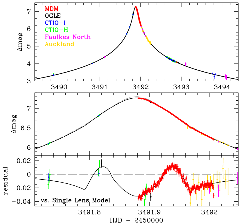
Figure 1: The light curve peak of event OGLE-2005-BLG-169 with photometric measurements from the MDM 2.4m $I$-band (red, Stanek reduction), OGLE $I$-band (black), CTIO $I$ and $H$-bands (blue and green), Faulkes Telescope North (magenta), and the Auckland unfiltered telescope (gold). The best fit model is indicated by the black curve, and the grey dashed curve indicates the same model without the planetary signal. The bottom panel shows the residual with respect to this no-planet model. The MDM data clearly trace out the caustic exit feature, but the data on the rising side provide a very weak constraint on the caustic entry properties. So, a variety of angles between the lens axis and the source trajectory are permitted by the photometry. The best fit model to the data set including the Stanek MDM photometry presented here is consistent with our proper motion measurement, while the light curve presented in Gould et al. (2006) is not.

In addition to the MDM data set, which contains the planetary signal, the photometry for this event include data from the $1.3\,$m OGLE survey telescope (responsible for the identification of the microlensing event), the $1.3\,$m SMARTS telescope at CTIO in Chile, the $2.0\,$m Faulkes Telescope North in Hawaii, and the $0.35\,$m Nustrini Telescope in Auckland, New Zealand. We use the same photometric reduction for each data set that was used by Gould et al. (2006) except for the CTIO data. A minor problem was discovered in the CTIO $I$-band photometry used in the original paper. The CTIO $I$-band photometry yielded a source magnitude that was $0.13\,$mag fainter than the source magnitude from the OGLE $I$-band photometry when the photometry from both data sets was calibrated to the OGLE-III photometry database (Szymański et al., 2011). This inconsistency was largely resolved (reduced to $0.03\,$mag) by switching from DoPHOT (Schechter, Mateo, & Saha, 1993) to SoDoPHOT photometry (Bennett et al., 1993). In this analysis, we have also included the CTIO $H$-band data, taken simultaneously with the $V$ and $I$-band data on the Andicam instrument on the SMARTS telescope. The $H$-band data is especially useful because they allow a more precise determination of the angular source radius (Kervella et al., 2004; Boyajian et al., 2014). The $H$-band light curve used in this paper is a SoDoPHOT reduction, but a reduction using the MOA Collaboration difference imaging pipeline (Bond et al., 2001) gives indistinguishable results.

3 Light Curve Models

The light curve models used for this paper are different from the models presented in Gould et al. (2006) because a different data set is used. We use the Bennett (2010) modeling code instead of the Gould et al. (2006) code, but this has no effect on the results, as these codes have been shown to give identical results to better than 1 part in $10^{4}$. Our conclusions based on the light curve modeling alone are essentially the same as the conclusions of Gould et al. (2006) . As discussed in Gould et al. (2006) and Section 2, the planetary signal for this event is particularly sensitive to potential systematic photometry errors because of the larger than usual S/N of the MDM observations and the small amplitude of the planetary signal. For this reason, Gould et al. (2006) did the complete analysis using both the Stanek and OGLE-pipeline photometry. We continue this philosophy in this paper and assume that the OGLE-pipeline and Stanek reductions are equally likely to be correct, and so we perform Markov Chain Monte Carlo (MCMC) calculations for both data sets starting at the parameters of each of the local $\chi^{2}$ minima presented in Gould et al. (2006).

The results of these MCMC calculations differ in detail from the results presented in Gould et al. (2006), in the sense that the models with the source trajectory nearly perpendicular to the lens axis are now somewhat favored with respect to the previous analysis. With the Stanek version of the MDM photometry, these models are now favored by $\Delta\chi^{2}=8.8$ over the best fit model with a source trajectory $>25^{\circ}$ from perpendicular to the lens axis. The best fit model using the Stanek version of the MDM photometry is presented in Figure 1, and the parameters of this model and the best fit $s<1$ model are given in Table 1. The best fit model, which has $s>1$, is labeled as “Stanek $s>1$,” and the parameters of the best fit $s<1$ are also given. This $s<1$ model is very slightly disfavored with $\Delta\chi^{2}=0.12$. Table 1 also gives the MCMC averages of the parameters both without the constraints from the HST measurements (in the next-to-last column) and with the constraints from the HST measurements in the last column. Because of the wide variation in the $\theta$ values (source trajectory angles) allowed by the light curve, there is a large scatter in some of the other fit parameters, such as the source radius crossing time, $t_{*}$, and the planet:star mass ratio, $q$.

Table 1: Model Parameters

				MCMC averages
parameter	units	Stanek $s>1$	Stanek $s<1$	no const.	${\mbox{\boldmath$\bf\mu$}}_{\rm rel,H}$ const.
$t_{E}$	days	43.09	43.16	41.8(2.9)	42.5(1.4)
$t_{0}$	${\rm HJD}-2453490$	1.8784	1.8784	1.8776(10)	1.8784(1)
$u_{\rm min}$		0.001229	0.001228	0.001267(9)	0.001250(4)
$s$		1.0190	0.9828	1.004(18)	1.001(18)
$\theta$	radians	1.6025	1.6069	1.43(20)	1.60(3)
$q$	$10^{-5}$	5.913	5.844	7.07(1.22)	6.15(30)
$t_{\ast}$	days	0.02174	0.02168	0.0202(17)	0.0228(5)
$\theta_{E}$	mas	0.905	0.911	0.965(94)	0.848(27)
$\mu_{\rm rel,G}$	mas/yr	7.67	7.69	8.47(87)	7.29(15)
$H_{s}$		18.852	18.854	18.81(8)	18.84(4)
$I_{s}$		20.592	20.594	20.55(8)	20.58(4)
$V_{s}$		22.254	22.257	22.21(8)	22.24(4)
fit $\chi^{2}$		1146.66	1146.78

Figure 2: The caustic configuration for the OGLE-2005-BLG-169 model shown in Figure 1. The black line, with arrow, shows the source trajectory for this model, while the grey dashed line shows the source trajectory for the other local $\chi^{2}$ minimum for the light curve modeling. This and similar models are consistent with the light curve, but they are contradicted by the relative proper motion measurement that we present here.

Figure 2 shows a close-up of the caustic configuration for the best-fit model with the source trajectory given by the solid black line. The red circle indicates the size of the source star, and the gray dashed line shows the source trajectory for the model presented in Gould et al. (2006).

4 Calibration and Source Radius

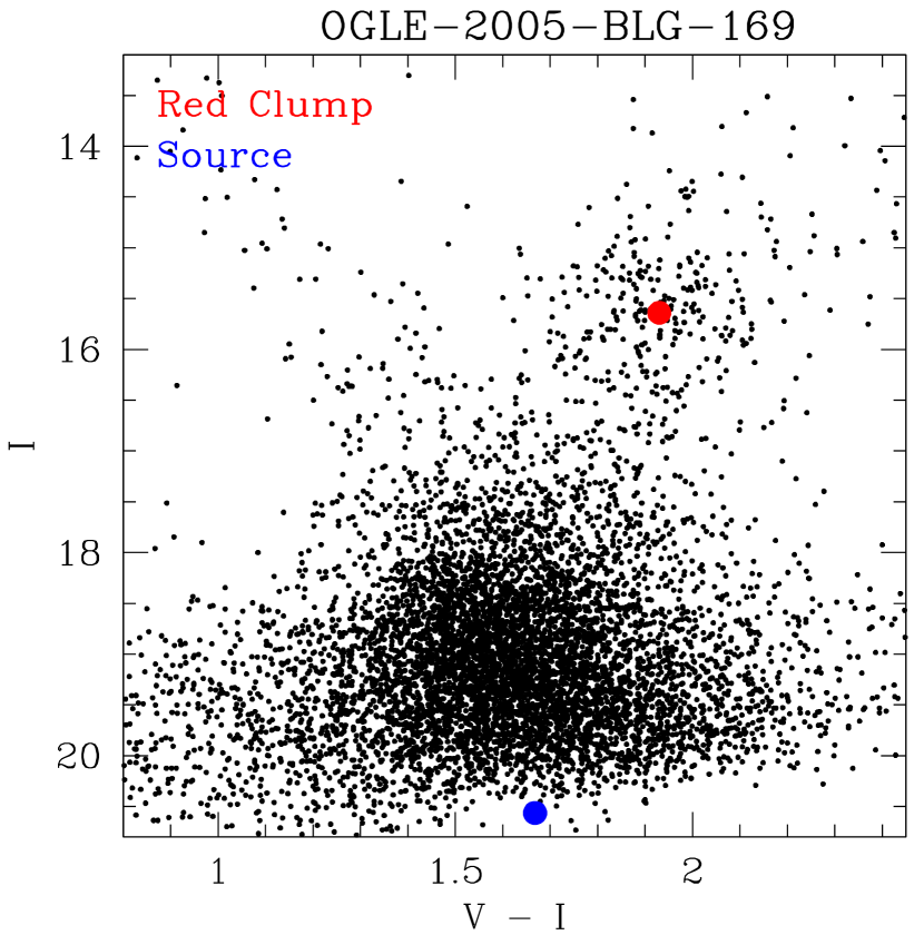
Figure 3: The $(V-I,I)$ color magnitude diagram (CMD) of the stars in the OGLE-III catalog (Szymański et al., 2011) within $120^{\prime\prime}$ of OGLE-2005-BLG-169. The red spot indicates red clump giant centroid, and the blue spot indicates the source magnitude and color.

In order to measure the angular Einstein radius, $\theta_{E}=\theta_{\ast}t_{E}/t_{\ast}$, we must determine the angular radius of the source star, $\theta_{\ast}$, from the dereddened brightness and color of the source star (Kervella et al., 2004; Boyajian et al., 2014). We determine the source star brightness in the $V$ and $I$-bands by calibrating the CTIO $V$-band and OGLE $I$-band magnitudes to the OGLE-III catalog (Szymański et al., 2011) yielding the following relations:

$$V_{\rm O3cal} =23.08516+0.97257\,V_{\rm Sod}+0.02743\,I_{\rm O3lc}\pm 0.004$$ (1)

$$I_{\rm O3cal} =1.406255+0.93933\,I_{\rm O3lc}+0.060674\,V_{\rm Sod}\pm 0.004\ .$$ (2)

$I_{\rm O3lc}$ is the OGLE $I$-band light curve magnitude, which differs from the standard Cousins $I$-band used in the OGLE-III catalog, while $V_{\rm O3cal}$ and $I_{\rm O3cal}$ refer to the Johnson $V$-band and Cousins $I$-band magnitudes, as presented in the OGLE-III catalog (Szymański et al., 2011). $V_{\rm Sod}$ is the raw CTIO $V$-band photometry from our SoDoPHOT reduction. The $V$-band calibration is based on 54 stars with $1.0\leq(V-I)_{\rm O3cal}<2.2$ and $I_{\rm O3cal}\leq 16.0$ within 2 arc minutes of the target star, and the $I$-band calibration employs the formulae presented in Szymański et al. (2011).

Our CTIO $H$-band SoDoPHOT magnitudes are calibrated to 2MASS (Carpenter, 2001) with the following relation,

$$H_{\rm 2mass}=H_{\rm Sod}+19.849\pm 0.010\ ,$$ (3)

based on 36 stars within $105^{\prime\prime}$ of the target.

In order to estimate the source radius, we need extinction-corrected magnitudes, and we determine these from the magnitudes and colors of the centroid of the red clump giant feature in the color magnitude diagram (CMD), as indicated in Figure 3. The extinction can be determined most accurately if three colors are used (Bennett et al., 2010), and we find that the red clump centroid in this field is at $I_{\rm cl}=15.61$, $(V-I)_{\rm cl}=1.93$, $(I-H)_{\rm cl}=2.07$, which implies $H_{\rm cl}=13.54$ and $V_{\rm cl}=17.54$.

We follow the method of Bennett et al. (2010) to determine the extinction, but we use the updated dereddened red clump magnitudes of Nataf et al. (2013). We assume absolute red clump giant centroid magnitudes of $M_{H\rm cl}=-1.30$, $M_{I\rm cl}=-0.13$, and $M_{V\rm cl}=0.93$. The Galactic coordinates of OGLE-2005-BLG-169 are $(l,b)=(0.6769^{\circ},-4.7402^{\circ})$, and this implies a distance modulus of $DM=14.541$. Using the Bennett et al. (2010) method, we estimate the extinction toward the center of the Galaxy in this direction to be $A_{H}=0.374\pm 0.020$, $A_{I}=1.256\pm 0.050$, and $A_{V}=2.132\pm 0.090$. These extinction values allow us to determine the dereddened magnitude for each passband, $C_{s0}=C_{s}-A_{C}$ where $C$ refers to the passband (either $V$, $I$, or $H$).

These dereddened magnitudes can be used to determine the angular source radius, $\theta_{*}$. Of the measured source magnitudes, the most precise determination of $\theta_{*}$ comes from the $(V-H),H$ relation. We use

$$\log_{10}\left[2\theta_{*}/(1{\rm mas})\right]=0.536654+0.072703\,(V-H)_{s0}-0.2\,H_{s0}\ ,$$ (4)

which comes from the Boyajian et al. (2014) analysis. These numbers are not included in the Boyajian et al. (2014) paper, but they were provided in a private communication from T.S. Boyajian (2014). She reports that this formula determines $\theta_{*}$ better than 2% accuracy. This is somewhat better than the 2.6% accuracy of the $(V-H),H$ relation of Kervella et al. (2004). (They report an accuracy of 1.12% for $\log_{10}(\theta_{*})$, which corresponds to 2.6% accuracy for $\theta_{*}$.)

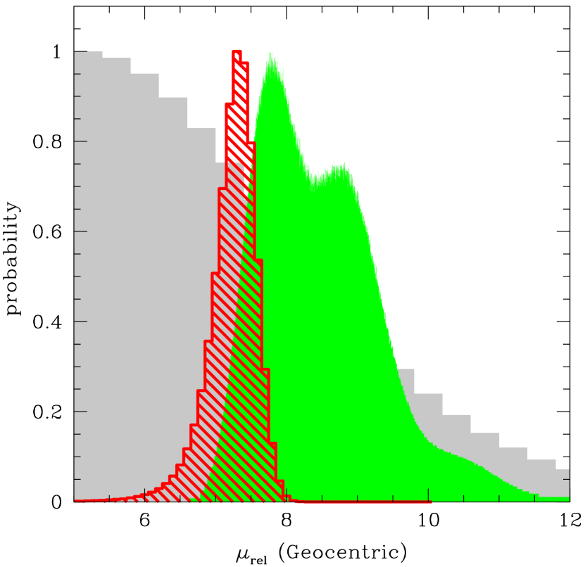
Figure 4: Comparison of geocentric proper motion predictions from all Galactic bulge microlensing events (grey histogram), microlensing models consistent with the light curve data (green histogram) and with the HST measurement (red cross-hatched histogram). The light curve $\mu_{\rm rel,G}$ distribution is drawn from MCMC calculations using both the Stanek and OGLE MDM reductions. The HST $\mu_{\rm rel,G}$ distribution has been converted from the two-dimensional ${\mbox{\boldmath$\bf\mu$}}_{\rm rel,H}$ measurement using a probability distribution for relative lens distance ($D_{L}/D_{S}$) from a Galactic model.

The implied source radii for the best fit $s>1$ and $s<1$ models are given in Table 1, along with the angular Einstein radius, $\theta_{E}$, and the lens-source relative proper motion, $\mu_{\rm rel,G}=\theta_{*}/t_{*}$, in a geocentric reference frame. The light curve parameter that the relative proper motion depends on is the source radius crossing time, $t_{*}$, which is measured in the reference frame of the Earth-bound observatories that observe the light curve. So, $t_{*}$ is measured the Geocentric reference frame moving at the instantaneous velocity of the Earth at the time of the event, and this is the reference frame that $\mu_{\rm rel,G}$ is determined in. The green histogram in Figure 4 shows the distribution of $\mu_{\rm rel,G}$ from our MCMC light curve modeling calculations using both the Stanek and OGLE-pipeline reductions of the MDM data. The spread in $\mu_{\rm rel,G}$ values is primarily due to the uncertainty in the source trajectory angle, $\theta$, as discussed in Section 3.

In Section 5, we will present the relative lens-source proper motion measurement from the HST observations. This measurement is made with respect to the average motion of the Earth during the 6.4678 years between the event and the HST observations. If we assume that the HST observations are made in a Heliocentric frame, the maximum error in the lens-source displacement is twice the relative lens-source relative parallax or $2\pi_{\rm rel}=2{\rm AU}(1/D_{L}-1/D_{S})\simeq 0.26$ (assuming our final result), which compares to our lens-source displacement measurement error of $1.3\,$mas, so the assumption of a Heliocentric reference frame is a reasonable approximation. (The lens-source relative parallax is given by $\pi_{\rm rel}={\rm AU}\left(D_{L}^{-1}-D_{S}^{-1}\right)$. ) The HST measurements also determine the direction of the lens-source relative proper motion, so they determine the 2-dimensional relative proper motion, ${\mbox{\boldmath$\bf\mu$}}_{\rm rel,H}$.

5 HST Astrometry and Photometry

We observed the OGLE-2005-BLG-169 source and lens stars for two HST orbits as a part of HST Program GO-12541. On 2011 October 19, we obtained images in three passbands, F814W, F555W, and F438W, using the Wide Field Camera 3-Ultraviolet-Visible (WFC3-UV) instrument. We obtained $7\times 85\,$sec dithered F814W exposures, $8\times 175\,$sec dithered F555W exposures, and $6\times 349\,$sec dithered F438W exposures. Due to the relatively short exposure times, we have been forced to limit the amount of data read out for the F555W and F814W exposures. Only 1k$\times$1k region of the CCDs were read out for these passbands.

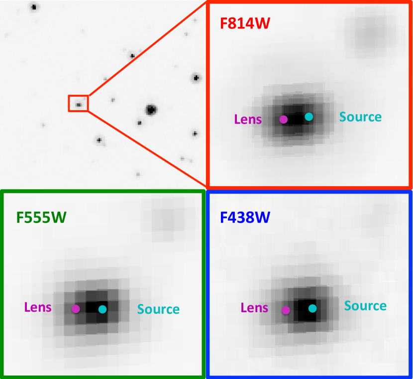
Figure 5: The top-left panel shows a $4.9^{\prime\prime}\times 4.6^{\prime\prime}$ section of the stacked F814W images containing the target, and the top-right panel shows a close-up of a $0.42^{\prime\prime}\times 0.37^{\prime\prime}$ region containing the lens and source stars. The lower-left and lower-right panels show the same region using the stacked images in the F555W and F438W passbands. The magenta spots on the left are the best fit lens locations and the cyan spots on the right are the best fit source positions. These close-up images are sums of all the dithered images with $100\times$ oversampling. The distortion of the WFC3 images has been removed, and this results in pixels shaped like parallelograms rather than squares.

The data were reduced following the method of Anderson & King (2000, 2004). The dithered exposures are used to construct an effective PSF from stars of a similar color to the target (i.e. the blended image of the source plus lens stars). Then, this effective PSF is used to fit two stellar profiles to the blended target image. The top-right and bottom two panels of Figure 5 show close-ups of the blended source plus lens stars in the three passbands, F814W, F555W, and F438W, which are the HST versions of the $I$, $V$, and $B$-bands. The best fit locations of the lens and source stars are also indicated. In the F814W images, both the stars have a brightness consistent with $I$-band source brightness determined from light curve modeling, so there would be ambiguity in the lens and source star identifications if we had data in this passband alone. Fortunately, the lens is considerably fainter than the source in the F555W and F438W passbands, and this allows us to uniquely identify the lens and source stars. (The lens is closer than the main sequence source, so it must be redder than the source if it has the same magnitude in the $I$-band.)

The separation between the lens and source stars is due to the $\Delta t=6.4678\,$yr interval between the event and the HST observations, so we can determine the relative proper motion in the Heliocentric frame by ${\mbox{\boldmath$\bf\mu$}}_{\rm rel,H}=\mbox{\boldmath$\bf\Delta x$}/\Delta t$, where $\bf\Delta x$ is the two-dimensional separation between the lens and source stars as measured in the HST images. In the Galactic coordinate system, we find

$${\mbox{\boldmath$\bf\mu$}}_{\rm rel,H}(l,b) =(7.52\pm 0.27,1.07\pm 0.28)\,{\rm mas/yr}\ \ ({\rm F814W})\ ,$$ (5)

$${\mbox{\boldmath$\bf\mu$}}_{\rm rel,H}(l,b) =(7.17\pm 0.33,1.88\pm 0.41)\,{\rm mas/yr}\ \ ({\rm F555W})\ ,$$ (6)

$${\mbox{\boldmath$\bf\mu$}}_{\rm rel,H}(l,b) =(7.32\pm 0.67,1.40\pm 0.82)\,{\rm mas/yr}\ \ ({\rm F438W})\ .$$ (7)

The error bars for these ${\mbox{\boldmath$\bf\mu$}}_{\rm rel,H}$ values are determined from the dual star fits. First the fit $\chi^{2}$ values are renormalized to give $\chi^{2}/{\rm d.o.f.}=1$. The original $\chi^{2}/{\rm d.o.f.}$ values were 1.25, 1.64, and 1.39 for the F814W, F555W, and F438W passbands, respectively. Then, we add $0.1\,$mas/yr in quadrature and multiply the error bars by 1.5. These adjustments are meant to account for systematic uncertainties in the PSF models, and they ensure that values from the different passbands are consistent. (The systematic errors could probably be reduced by constructing different PSF models for the lens and source stars rather than one PSF based on their average color.) Note that the F438W and the Keck $H$-band (Batista et al., 2015) proper motion values both fall in between the F814W and F555W values, so there is no trend with color. We combine the best two measurements from equations 5-7 (F814W and F555W), to obtain the measurement we will use as our final measurement of the lens-source relative proper motion

$${\mbox{\boldmath$\bf\mu$}}_{\rm rel,H}(l,b)=(7.39\pm 0.20,1.33\pm 0.23)\,{\rm mas/yr}\ .$$ (8)

The direction of proper motion is about $\sim 10^{\circ}$ from the Galactic longitude, $l$, direction. This is expected for a Galactic disk lens about half way to the center of the Galaxy. Due to the Galaxy’s flat rotation curve, we and the lens system move at about the same velocity, but the source star in the Galactic bulge doesn’t share this rotation, so the relative lens-source proper motion is typically $\mu_{\rm rel}\approx 220\,{\rm km/s}/8.3\,{\rm kpc}=5.6\,$mas in the direction of Galactic rotation. The velocity dispersion is dominated by the Galactic bulge one-dimensional velocity dispersion of $\sim 100\,$km/s, which implies a one-dimensional proper motion dispersion of $2.5\,$mas/yr. So typically, the relative proper motion of lens half way to the bulge should be within $\sim 30^{\circ}$ of the Galactic rotation direction, while an event like OGLE-2005-BLG-169, with a higher than average $\mu_{\rm rel}$, would typically have a relative proper motion within $\sim 30^{\circ}$ of the Galactic rotation direction.

These fits also return the magnitudes of the source and lens stars. To put these on a standard scale, we calibrate the $V$ (F555W) and $I$ (F814W) to the OGLE-III catalog (Szymański et al., 2011). We find 12 uncrowded stars with $0.86<V-I<2.24$ and $I<19$ that we use for this calibration. The scatter in these calibrations are about $1\,$%, so the formal uncertainty in the calibration is 0.3-$0.4\,$%.

With this calibration, the best fit $V$ and $I$ source magnitudes are

$$V_{S}= 22.212\pm 0.041\ \ \ \ I_{S}=20.555\pm 0.054$$ (9)

$$V_{L}= 22.783\pm 0.067\ \ \ \ I_{L}=20.493\pm 0.051$$ (10)

$$V_{\rm tot}= 21.704\pm 0.020\ \ \ \ \ I_{\rm tot}=19.771\pm 0.020,$$ (11)

where $V_{\rm tot}$ and $I_{\rm tot}$ refer to the magnitudes corresponding to the combined brightness of the lens plus source stars. The formal errors on $V_{\rm tot}$ and $I_{\rm tot}$ are actually only about $0.003\,$mag, but we use 0.020 mag to account for calibration uncertainties. The uncertainties on the source and lens magnitudes are significantly larger than the uncertainty on the combined lens+source magnitude. This is due to the fact that the lens and source are not fully resolved, which allows correlated uncertainties where the lens and source can trade flux with slight modifications in their best fit positions.

The F438W data were calibrated to the Vega-magnitude scale by comparison to a reduction of the same data using DolPHOT, which is an updated version of HSTphot (Dolphin, 2000) by the same author. This gives $B_{S}=23.82\pm 0.06$ and $B_{L}=24.74\pm 0.15$.

5.1 Confirmation of Planetary Signal Prediction

Our HST measurements of the lens-source relative proper motion, ${\mbox{\boldmath$\bf\mu$}}_{\rm rel,H}$, are made in a reference frame that is indistinguishable from the Heliocentric reference frame, but the light curve measurements are made in the Geocentric reference frame that moves with the Earth at the time of the event. These reference frames differ by the velocity of the Earth at the time of the event projected onto the plane of the sky at the time of the event. This projected velocity is

$$(v_{\oplus N},v_{\oplus E})=(3.15,18.51)\,{\rm km/sec}=(0.665,3.905)\,{\rm AU/yr}\ ,$$ (12)

and the relationship between the geocentric and heliocentric relative proper motions is

$${\mbox{\boldmath$\bf\mu$}}_{\rm rel,H}={\mbox{\boldmath$\bf\mu$}}_{\rm rel,G}+{\pi_{\rm rel}\over{\rm AU}}{\mbox{\boldmath$\bf v$}}_{\oplus}\ .$$ (13)

Converting to Galactic coordinates, we have $(v_{\oplus l},v_{\oplus b})=(3.74,-1.30)\,$AU/yr, so equation 13 becomes

$${\mbox{\boldmath$\bf\mu$}}_{\rm rel,G}(l,b)={\mbox{\boldmath$\bf\mu$}}_{\rm rel,H}(l,b)+{\pi_{\rm rel}\over{\rm yr}}(-3.74,1,30)\\$$ (14)

in Galactic coordinates or

$${\mbox{\boldmath$\bf\mu$}}_{\rm rel,G}(l,b)=(7.39,1.33)+{\pi_{\rm rel}\over 0.13\,{\rm mas}}(-0.49,0.17)\ ,$$ (15)

after substituting our measured value from equation 8. We choose $\pi_{\rm rel}=0.13\,$mas as our reference value in equation 15 because this is a round number close to our best fit final value. It corresponds to a lens system at a distance of about $4\,$kpc, about half-way to the Galactic center.

However, we’d like to compare our measurement of ${\mbox{\boldmath$\bf\mu$}}_{\rm rel,H}$ to the light curve prediction of $\mu_{\rm rel,G}$ with no reference to our best fit lens distance, in order to have a relatively pure test of the relative proper motion prediction from the light curve. We therefore convert the measured Heliocentric relative proper motion measurement to a probability distribution for $\mu_{\rm rel,G}$ using a Bayesian analysis with the Galactic model of Bennett et al. (2014). This analysis implicitly assumes that potential primary lens mass for the OGLE-2005-BLG-169 event is equally likely to host a planet with the measured mass ratio, but it makes no assumptions about the location of the lens system or source star.

The red cross-hatched histogram in Figure 4 indicates the distribution of $\mu_{\rm rel,G}$ values consistent with the HST ${\mbox{\boldmath$\bf\mu$}}_{\rm rel,H}$ measurement. The HST values for $\mu_{\rm rel,G}$ are near the extreme low-$\mu_{\rm rel,G}$ edge of the light curve distribution, shown in green. However, the histograms cross at a probability of about 80% of the maximum of each curve. Thus, the HST measurement is clearly consistent with the $\mu_{\rm rel,G}$ predictions from the light curve.

The light curve prediction of $\mu_{\rm rel,G}$ comes directly from the planetary light curve feature, because this is the only light curve feature that resolves the finite source size and determines the source radius crossing time, $t_{*}$. Thus, our HST confirmation of the $\mu_{\rm rel,G}$ is also a confirmation of the planetary interpretation of the OGLE-2005-BLG-169 light curve. This is the first such confirmation for a planetary microlensing event.

5.2 Comparison to Keck Adaptive Optics Measurements

In July, 2013, a subset of us obtained 15 Keck NIRC2 Adaptive optics $H$-band images with seeing of $\sim 55\,$mas. These high resolution images resolved the lens and source stars, so that their separation could be measured, some $8.2121\,$years after the microlensing event peak. This allowed an independent measurement of the lens-source relative proper motion (Batista et al., 2015),

$${\mbox{\boldmath$\bf\mu$}}_{\rm rel,H}(l,b)[{\rm Keck}]=(7.28\pm 0.12,1.54\pm 0.12)\,{\rm mas/yr}\ .$$ (16)

This measurement is obviously quite consistent with our HST measurement given above (equation 8) as both the $l$ and $b$ components are within 1-$\sigma$ of our values.

Both of these ${\mbox{\boldmath$\bf\mu$}}_{\rm rel,H}$ measurements make the assumption that the lens and source are coincident during the microlensing event, but we can also use the $1.7443\,$yr interval between the HST and Keck observations to work out the separation at the time of the event between the stars we identify as the lens and source. This gives a separation of

$$(\Delta l,\Delta b)=(3.5\pm 7.2,-6.4\pm 7.8)\,{\rm mas}\ ,$$ (17)

between these lens and source stars at the time of the event. These are consistent at $<1\,\sigma$ with our identification of the lens and source stars, whose separation was $\theta_{E}u_{\rm min}=0.0011\,$mas at the time of the event.

This measurement is also sufficient to rule out the possibility that the detected flux is due to a binary companion to the lens. A possible binary companion to the lens that orbits within $30\,$mas of the primary lens star would strongly perturb the light curve, so such a close companion is excluded by the light curve observations, which see no evidence of such a companion (Bennett et al., 2007; Gould, 2014). Thus, this light curve constraint combined with the combined Keck+HST measurements, excludes the possibility that a binary companion to the lens is responsible for the flux that we attribute to the lens stars.

5.3 Lens System Properties from HST Measurements

As discussed in Section 4, the angular Einstein radius, $\theta_{E}=\theta_{*}t_{E}/t_{*}$, can be determined from light curve parameters, as long as the angular source size, $\theta_{*}$, can be determined from the source brightness and color. The determination of $\theta_{E}$ allows us to use the following relation (Bennett, 2008; Gaudi, 2012)

$$M_{L}={c^{2}\over 4G}\theta_{E}^{2}{D_{S}D_{L}\over D_{S}-D_{L}}={c^{2}\over 4G}\theta_{E}^{2}{{\rm AU}\over\pi_{\rm rel}}=0.9823\,M_{\odot}\left({\theta_{E}\over 1\,{\rm mas}}\right)^{2}\left({x\over 1-x}\right)\left({D_{S}\over 8\,{\rm kpc}}\right)\ ,$$ (18)

where $x=D_{L}/D_{S}$. This expression can be considered to be a mass-distance relation, since $D_{S}$ is approximately known. As can be seen from Table 1, the light curve does not determine $\theta_{E}$ very precisely, due to the correlated uncertainty in $\theta$ and $t_{*}$. However, as Figure 4 indicates, the HST observations rule out a large fraction of the $\mu_{\rm rel,G}$ values that are compatible with the light curve. Since $\theta_{E}=\mu_{\rm rel,G}t_{E}$, this implies that much of the $\theta_{E}$ range allowed by the light curve is now excluded by the HST data. This, in turn, has an effect on other parameters, such as the planet:star mass ratio, which is $q\approx 6\times 10^{-5}$ for the $\theta\approx 1.6$ solutions, compared to $q\approx 8\times 10^{-5}$ for the $\theta\approx 1.0$ solutions. So, the HST data drive the planetary mass fraction to a somewhat lower value.

Table 2: Physical Parameters

Parameter	units	value	2-$\sigma$ range
$D_{L}$	kpc	$4.1\pm 0.4$	3.3-4.8
$M_{\star}$	$M_{\odot}$	$0.69\pm 0.02$	0.64-0.73
$m_{p}$	${M_{\oplus}}$	$14.1\pm 0.9$	12.4-15.9
$a_{\perp}$	AU	$3.5\pm 0.3$	2.9-4.0
$a_{3d}$	AU	$4.0{+2.2\atop-0.6}$	3.0-14.0

Note. — Uncertainties are 1-$\sigma$ parameter ranges.

To solve for the planetary system parameters, we sum over our MCMC results as in Subsection 5.1 with the weighting by the Galactic model parameters consistent with the HST ${\mbox{\boldmath$\bf\mu$}}_{\rm rel,H}$ measurement, but now we add the HST lens brightness constraints, as well. In this sum, we randomly select source and lens distances that are consistent with the mass-distance relation (equation 18). In order to check this consistency, we must invoke a mass-luminosity relation. We use the mass-luminsity relations of Henry & McCarthy (1993), Henry et al. (1999) and Delfosse et al. (2000). For $M_{L}>0.66\,M_{\odot}$, we use the Henry & McCarthy (1993) relation; for $0.12\,M_{\odot}<M_{L}<0.54\,M_{\odot}$, we use the Delfosse et al. (2000) relation; and for $0.07\,M_{\odot}<M_{L}<0.10\,M_{\odot}$, we use the Henry et al. (1999) relation. In between these mass ranges, we linearly interpolate between the two relations used on the boundaries. That is we interpolate between the Henry & McCarthy (1993) and the Delfosse et al. (2000) relations for $0.54\,M_{\odot}<M_{L}<0.66\,M_{\odot}$, and we interpolate between the Delfosse et al. (2000) and Henry et al. (1999) relations for $0.10\,M_{\odot}<M_{L}<0.12\,M_{\odot}$.

At a Galactic latitude of $b=-4.7402^{\circ}$, and a lens distance of $\sim 4\,$kpc, the lens system is likely to be behind most, but not all, of the dust that is in the foreground of the source. We assume a dust scale height of $h_{\rm dust}=0.10\pm 0.02$kpc, so that the extinction in the foreground of the lens is given by

$$A_{i,L}={1-e^{-|D_{L}/(h_{\rm dust}\sin b)|}\over 1-e^{-|D_{S}/(h_{\rm dust}\sin b)|}}A_{i,S}\ ,$$ (19)

where the index $i$ refers to the passband: $V$, $I$, or $H$. For each model in the Markov Chain, the $h_{\rm dust}$ value is selected randomly from a Gaussian distribution. We assume error bars of $\sigma_{V}=0.10$ and $\sigma_{I}=0.07$ magnitudes for the combined uncertainty in the mass-luminosity relations and the lens star extinction estimate. The results of this final sum over the Markov Chain are given in Table 2. The host star is a $M_{\star}=0.69\pm 0.02\,M_{\odot}$ K-dwarf, orbited by a planet of about Uranus’ mass at $m_{p}=14.1\pm 0.9\,{M_{\oplus}}$, at a projected separation of $a_{\perp}=3.5\pm 0.3\,$AU. Assuming a random orientation, this implies 3-dimensional separation of $a_{3d}=4.0{+2.2\atop-0.6}\,$AU. This planet then has the mass of an ice-giant in a Jupiter-like orbit at about twice the nominal snow-line distance of $2.7(M/M_{\odot})\,{\rm AU}\simeq 1.9\,$AU. This is similar to a number of other planets found by microlensing (Beaulieu et al., 2006; Sumi et al., 2010; Muraki et al., 2011; Furusawa et al., 2013), which can be interpreted as examples of “failed Jupiter cores.” These would be planets that grew by accumulation of solids, as Jupiter’s core is thought to have done (Lissauer, 1993), if the core accretion model is correct. These “failed Jupiter core” planets are thought to be common around the low-mass stars probed by the microlensing exoplanet search method.

6 Discussion and Conclusions

We report the first detection of an exoplanet microlens host star found at the separation predicted by the exoplanet feature in the microlensing light curve. Together with a companion paper based on Keck data (Batista et al., 2015), this provides the first confirmation of a microlensing planetary signal, in the sense that the planetary interpretation of a light curve feature predicted the lens-source relative proper motion, which we, and Batista et al. (2015) have confirmed.

The resulting system is a Uranus-mass planet orbiting a K-dwarf at about twice the snow-line, which fits the properties of a “failed Jupiter core” planet, predicted by core accretion (Laughlin et al., 2004).

This is also the first demonstration of the primary exoplanet host star mass measurement method (Bennett et al., 2007) planned for WFIRST (Spergel et al., 2013) and EUCLID (Penny et al., 2013). While, the host star mass might plausibly be inferred from just the brightness of the lens star (Bennett et al., 2006; Dong et al., 2009; Batista et al., 2014), but to be highly confident that the measured star is actually the lens star (Janczak et al., 2010), it is necessary to measure the lens-source relative proper motion and show that it is consistent with the prediction from the light curve. This will be even more important for the WFIRST exoplanet microlensing survey, because it will work in more crowded fields, where the microlensing rate is highest.

The HST data presented her provide an extremely high S/N measurement of the lens-source relative proper motion. The lens-source separation is measured at 28-$\sigma$ in the F814W band, 22-$\sigma$ in the F555W band, and 11-$\sigma$ in the F438W band. This is partly because this event is a favorable one for such measurement (Henderson et al., 2014), but also because it took a while for the HST TAC to recognize the importance of such measurements. As discussed in Bennett et al. (2007), this measurement could easily have been made 4 years earlier.

It was not necessary to achieve the photon noise limit in our HST astrometry measurements because of the high S/N in the HST data. As the discussion in Section 5 indicates, our error bars are probably about a factor of two above the photon noise limit. There are several things that can be done to improve the analysis. One improvement would be to add a second iteration of PSF fitting to determine the source and lens properties. The first iteration determines the approximate source and lens colors, but the stars selected to make the PSF models are matched to the average lens+source color. In a second iteration, new PSF models could be make to match the lens and source star, and second round of fitting could be done with custom PSF models for the lens and source stars.

An additional improvement in the method would be to fit more than two sources in the HST images in the vicinity of the target star. In the close-ups in the top-right and bottom two panels of Figure 5, there is a faint star in the upper right corner. If this star were brighter or if the lens or source were much fainter, the PSF wings of this star could interfere with the lens and/or source star fits. The solution is then to also fit for that star. We expect to use this method for other targets that have been observed in Program GO-12541.

References

- Alard & Lupton (1998) Alard, C. & Lupton, R.H. 1998, ApJ, 503, 325
- Anderson & King (2000) Anderson, J. & King, I. R. 2000, PASP, 112, 1360
- Anderson & King (2004) Anderson, J. & King, I. R. 2004, Hubble Space Telescope Advanced Camera for Surveys Instrument Science Report 04-15
- Batista et al. (2014) Batista, V., Beaulieu, J.-P., Gould, A., et al. 2014, ApJ, 780, 54
- Batista et al. (2015) Batista, V., Beaulieu, J.-P., Bennett, D.P., et al. 2015, submitted.
- Beaulieu et al. (2006) Beaulieu, J.-P., Bennett, D. P., Fouqué, P., et al. 2006, Nature, 439, 437
- Bennett (2008) Bennett, D.P, 2008, in Exoplanets, Edited by John Mason. Berlin: Springer. ISBN: 978-3-540-74007-0, (arXiv:0902.1761)
- Bennett (2010) Bennett, D.P. 2010, ApJ, 716, 1408
- Bennett et al. (1993) Bennett, D. P., Alcock, C., Allsman, R., et al. 1993, Bulletin of the American Astronomical Society, 25, 1402
- Bennett et al. (2006) Bennett, D. P., Anderson, J., Bond, I. A., Udalski, A., & Gould, A. 2006, ApJ, 647, L171
- Bennett et al. (2007) Bennett, D.P., Anderson, J., & Gaudi, B.S. 2007, ApJ, 660, 781
- Bennett et al. (2014) Bennett, D. P., Batista, V., Bond, I. A., et al. 2014, ApJ, 785, 155
- Bennett et al. (2008) Bennett, D. P., Bond, I. A., Udalski, A., et al. 2008, ApJ, 684, 663
- Bennett et al. (2010) Bennett, D. P., Rhie, S. H., Nikolaev, S., et al. 2010, ApJ, 713, 837
- Bennett & Rhie (1996) Bennett, D.P. & Rhie, S.H. 1996, ApJ, 472, 660
- Bennett & Rhie (2002) Bennett, D.P. & Rhie, S.H. 2002, ApJ, 574, 985
- Bond et al. (2001) Bond, I. A., Abe, F., Dodd, R. J., et al. 2001, MNRAS, 327, 868
- Boyajian et al. (2014) Boyajian, T.S., van Belle, G., & von Braun, K., 2014, AJ, 147, 47
- Cardelli et al. (1989) Cardelli, J.A., Clayton, G.C., & Mathis, J.S. 1989, ApJ, 345, 245
- Carpenter (2001) Carpenter, J.M. 2001, AJ121, 2851
- Delfosse et al. (2000) Delfosse, X., Forveille, T., Ségransan, D., et al. 2000, A&A, 364, 217
- Dolphin (2000) Dolphin, A. E. 2000, PASP, 112, 1383
- Dong et al. (2009) Dong, S., Bond, I. A., Gould, A., et al. 2009, ApJ, 698, 1826
- Furusawa et al. (2013) Furusawa, K., Udalski, A., Sumi, T., et al. 2013, ApJ, 779, 91
- Gaudi (2012) Gaudi, B. S. 2012, ARA&A, 50, 411
- Gaudi et al. (2008) Gaudi, B. S., Bennett, D. P., Udalski, A., et al. 2008, Science, 319, 927
- Gould (2014) Gould, A. 2014, J. Kor. Ast. Soc., 47, 215
- Gould & Loeb (1992) Gould, A. & Loeb, A. 1992, ApJ, 396, 104
- Gould et al. (2006) Gould, A., Udalski, A., An, D., et al. 2006, ApJ, 644, L37
- Green et al. (2012) Green, J., Schechter, P., Baltay, C., et al. 2012, arXiv:1208.4012
- Hartman et al. (2004) Hartman, J. D., Bakos, G., Stanek, K. Z., & Noyes, R. W. 2004, AJ, 128, 1761
- Henderson et al. (2014) Henderson, C. B., Park, H., Sumi, T., et al. 2014, ApJ, 794, 71
- Henry et al. (1999) Henry, T. J., Franz, O. G., Wasserman, L. H., et al. 1999, ApJ, 512, 864
- Henry & McCarthy (1993) Henry, T. J., & McCarthy, D. W., Jr. 1993, AJ, 106, 773
- Ida & Lin (2005) Ida, S., & Lin, D.N.C. 2005, ApJ, 626, 1045
- Janczak et al. (2010) Janczak, J., Fukui, A., Dong, S., et al. 2010, ApJ, 711, 731
- Kaib et al. (2013) Kaib, N. A., Raymond, S. N., & Duncan, M. 2013, Nature, 493, 381
- Kennedy & Kenyon (2008) Kennedy, G. M., & Kenyon, S. J. 2008, ApJ, 673, 502
- Kennedy et al. (2006) Kennedy, G.M., Kenyon, S.J., & Bromley, B.C. 2006, ApJ650, L139
- Kervella et al. (2004) Kervella, P., Thévenin, F., Di Folco, E., & Ségransan, D. 2004, A&A, 426, 297
- Kubas et al. (2012) Kubas, D., Beaulieu, J. P., Bennett, D. P., et al. 2012, A&A, 540, A78
- Laughlin et al. (2004) Laughlin, G. Bodenheimer, P. & Adams, F.C. 2004, ApJ, 612, L73
- Lecar (2006) Lecar, M., Podolak, M., Sasselov, D., & Chiang, E. 2006, ApJ, 640, 1115
- Lissauer (1993) Lissauer, J.J. 1993, Ann. Rev. Astron. Ast., 31, 129
- Mao & Paczyński (1991) Mao, S., & Paczyński, B. 1991, ApJ, 374, L37
- Muraki et al. (2011) Muraki, Y., Han, C., Bennett, D. P., et al. 2011, ApJ, 741, 22
- Nataf et al. (2013) Nataf, D. M., Gould, A., Fouqué, P., et al. 2013, ApJ, 769, 88
- Nishiyama et al. (2009) Nishiyama, S., Tamura, M., Hatano, H., et al. 2009, ApJ, 696, 1407
- Penny et al. (2013) Penny, M. T., Kerins, E., Rattenbury, N., et al. 2013, MNRAS, 434, 2
- Pollack et al. (1996) Pollack, J. B., Hubickyj, O., Bodenheimer, P., et al. 1996, Icarus, 124, 62
- Schechter, Mateo, & Saha (1993) Schechter, P. L., Mateo, M., & Saha, A. 1993, PASP, 105, 1342
- Spergel et al. (2013) Spergel, D., Gehrels, N., Breckinridge, J., et al. 2013, arXiv:1305.5422
- Sumi et al. (2010) Sumi, T., Bennett, D. P., Bond, I. A. et al. 2010, ApJ, 710, 1641
- Szymański et al. (2011) Szymański, M. K., Udalski, A., Soszyński, I., et al. 2011, Acta Astron., 61, 83
- Thommes et al. (2008) Thommes, E.W., Matsumura, S., & Rasio F.A. 2008, Science, 321, 814
- Udalski (2003) Udalski, A. 2003, Acta Astron., 53, 291