Boosting the annihilation boost:
Tidal effects on dark matter subhalos and consistent luminosity modeling

Abstract

In the cold dark matter paradigm, structures form hierarchically, implying that large structures contain smaller substructures. These subhalos will enhance signatures of dark matter annihilation such as gamma rays. In the literature, typical estimates of this boost factor assume a concentration-mass relation for field halos, to calculate the luminosity of subhalos. However, since subhalos accreted in the gravitational potential of their host loose mass through tidal stripping and dynamical friction, they have a quite characteristic density profile, different from that of the field halos of the same mass. In this work, we quantify the effect of tidal stripping on the boost factor, by developing a semi-analytic model that combines mass-accretion history of both the host and subhalos as well as subhalo accretion rates. We find that when subhalo luminosities are treated consistently, the boost factor increases by a factor 2–5, compared to the typical calculation assuming a field-halo concentration. This holds for host halos ranging from sub-galaxy to cluster masses and is independent of the subhalo mass function or specific concentration-mass relation. The results are particularly relevant for indirect dark matter searches in the extragalactic gamma-ray sky.

I Introduction

If dark matter is made of weakly interacting massive particles, their self-annihilation may produce high-energy gamma rays Bringmann and Weniger (2012). Indirect searches for dark matter annihilation with gamma-ray telescopes are one of the promising probes of non-gravitational interactions of dark matter. In hierarchical structure formation, small structures form first and they merge into larger dark matter halos. Numerical simulations show that the distribution of dark matter particles in the halo is clumpy, with a substantial fraction being locked into substructures Klypin et al. (1999); Moore et al. (1999). Since the self-annihilation rate depends on dark matter density squared, presence of these subhalos will boost the gamma-ray signal.

There are two well-adopted methods to estimate the boost factor Kuhlen et al. (2012). The first is to phenomenologically extrapolate subhalo properties, i.e., power-law scaling relations between subhalos with a mass above a given threshold and their total luminosity, down to scales of the smallest subhalos (typically assumed to be on the order of Earth mass, although very sensitive to the exact particle physics model Profumo et al. (2006); *Bringmann:2009vf; *vandenAarssen:2012ag; *Diamanti:2015kma), e.g., Springel et al. (2008a). This approach yields very large boosts, on the order of $10^{2}$ ($10^{3}$) for galaxy (cluster) halos. but there is no guarantee that this phenomenological extrapolation over many orders of magnitude is still valid. In fact, this method is similar to a power-law extrapolation of the so-called concentration-mass relation. The second one relies on a concentration-mass relation that flattens toward lower masses. This behavior is favored analytically as well as from dedicated simulations (Bullock et al., 2001; *Diemand:2006ey; *Maccio':2008xb; *Prada:2011jf; *Ludlow:2013vxa; Anderhalden and Diemand, 2013; *Ishiyama:2014uoa; Correa et al., 2015). Studies following this approach (e.g., Pieri et al. (2008); *Kuhlen:2008aw; *Charbonnier:2011ft; *Nezri:2012tu; Sanchez-Conde and Prada (2014); Anderhalden and Diemand (2013)) typically conclude that the boost factors are much more modest, about an order-of-magnitude below the phenomenological extrapolations.

The latter method is believed to yield more realistic values for the boost factor due to subhalos ($B_{\rm sh}$). The boost is typically calculated as an integral of $({\mathrm{d}N}/{\mathrm{d}m})L_{\rm sh}(m)$ over the subhalo mass $m$, with ${\mathrm{d}N}/{\mathrm{d}m}$ the subhalo mass function as found in simulations and extrapolated down to the the minimal subhalo mass, and $L_{\rm sh}(m)$ the subhalo luminosity, which is a function of the concentration. However, as mentioned by Ref. Sanchez-Conde and Prada (2014), so far this method has not been used fully consistently, since the concentration-mass relation that goes into the calculation of $L_{\rm sh}(m)$ is that of field halos, which is not directly applicable to the subhalos. In the gravitational potential of its host halo, a subhalo is subject to mass loss by a tidal force, which tends to strip particles from outer regions of the subhalo Kazantzidis et al. (2004); Diemand et al. (2007a); Springel et al. (2008b). This effect will reduce the subhalo mass substantially, but keeps the annihilation rate almost unchanged, because the latter happens in the dense central regions dominantly. Consequently, subhalos are expected to be denser and more luminous than halos of equal mass in the field, and thus, the boost should be larger.

In this paper, by developing semi-analytic models, we investigate the effect of tidal stripping of subhalos and show that using the field halo concentration indeed results in a significant underestimation of the subhalo luminosity, and hence the annihilation boost factor. Therefore, we argue that this effect is extremely important in this context, and a consistent treatment of subhalo concentrations should always be adopted.

We note that there are alternative estimates of the boost factor that do not depend on the concentration-mass relation directly. Reference Kamionkowski et al. (2010) applies an analytic model for the probability distribution function of the halo density field including substructure. Reference Zavala and Afshordi (2014) uses a technique based on the stable clustering hypothesis and includes the effects of tidal disruption. Both of these are then matched to numerical simulations above the resolution scale. Finally, reference Serpico et al. (2012) uses the nonlinear power spectrum directly to calculate the so-called flux multiplier, which encapsulates the boost, and thereby the extragalactic dark matter annihilation flux.

We adopt cosmological parameters from 5-year WMAP results (Komatsu et al., 2009). Capital $M$ refers to the host halo mass and lower-case $m$ to subhalo mass. Quantities at redshift $z=0$ are denoted by subscript 0. Virial radius, $r_{\mathrm{vir}}$, is defined as the radius within which the average density of a halo is $\Delta_{\mathrm{c}}(z)\rho_{\mathrm{c}}(z)$, where $\Delta_{\mathrm{c}}$ is given by Ref. Bryan and Norman (1998) and $\rho_{\mathrm{c}}(z)$ is the critical density at redshift $z$. The virial mass is defined correspondingly.

II Density profile and gamma-ray luminosity

The total gamma-ray luminosity of a dark matter halo of mass $M$ is (e.g., (Strigari et al., 2007))

$$L(M) =[1+B_{\rm sh}(M)]L_{\rm host}(M),$$ (1)

$$B_{\rm sh}(M) =\frac{1}{L_{\rm host}(M)}\int\mathrm{d}m\frac{\mathrm{d}N}{\mathrm{d}m}L_{\rm sh}(m)[1+B_{\rm ssh}(m)],$$ (2)

with $m$ the subhalo mass, $B_{\rm sh}(M)$ the boost factor due to subhalos, $L_{\rm host}(M)$ and $L_{\rm sh}(m)$ the luminosities of the smooth component of the host halo and subhalos, respectively (both often parameterized by the Navarro-Frenk-White (NFW) or Einasto profile (Navarro et al., 1996; Graham et al., 2006a)). According to the state-of-the-art numerical simulations, the subhalo mass function (i.e., number of subhalos per unit mass interval) behaves as a power-law $\mathrm{d}N/\mathrm{d}m\propto m^{-\alpha}$, where $\alpha=1.9$–2, down to resolution scales (Diemand et al., 2007b; Springel et al., 2008b; Hellwing et al., 2015). The boost factor due to “sub-substructure” $B_{\rm ssh}(m)$ is either parametrized the same way as $B_{\rm sh}$ or often neglected.

Assuming that the density profile of the subhalos is characterized by the NFW function up to tidal radius $r_{\mathrm{t}}$ (beyond which all dark matter particles are completely stripped), the subhalo luminosity is given by $L_{\rm sh}(m)\propto\rho_{\mathrm{s}}^{2}r_{\mathrm{s}}^{3}[1-1/(1+c_{\mathrm{t}})^{3}]$, where $\rho_{\mathrm{s}}$ and $r_{\mathrm{s}}$ are the characteristic density and scale radius of the NFW profile, and $c_{\mathrm{t}}\equiv r_{\mathrm{t}}/r_{\mathrm{s}}$. In the literature where the effect of tidal stripping is ignored, one adopts the virial radius $r_{\rm vir}$ and virial concentration parameter $c_{\rm vir}=r_{\rm vir}/r_{\mathrm{s}}$ instead of $r_{\mathrm{t}}$ and $c_{\mathrm{t}}$, respectively.

III Order-of-magnitude estimate

We start with an order-of-magnitude estimate. Rather than using physics-driven models, we rely on phenomenological relations found in numerical simulations, where the effect of tidal stripping is automatically taken into account. Let us define $V_{\rm max}$ and $r_{\rm max}$ as the maximum circular velocity and radius where the velocity reaches $V_{\rm max}$. For the NFW profile, these quantities are related to $\rho_{\rm s}$ and $r_{\mathrm{s}}$ through $r_{\mathrm{s}}=r_{\rm max}/2.163$ and $\rho_{\rm s}=(4.625/4\pi G)(V_{\rm max}/r_{\mathrm{s}})^{2}$.

For field halos, we assume the concentration-mass relation from Ref. (Neto et al., 2007) that matches well the simulation results of Ref. Springel et al. (2008b) down to the resolution limit. For a field halo of mass $m_{\rm fh}=10^{5}\mathrm{\,M_{\odot}}$, we find $c_{\mathrm{vir}}\approx 63$. All other relevant quantities ($r_{\mathrm{vir}}$, $r_{\mathrm{s}}$, and $\rho_{\mathrm{s}}$) then follow from $m_{\rm fh}=4\pi\Delta_{c,0}\rho_{\rm c,0}r_{\mathrm{vir}}^{3}/3$, $r_{\mathrm{s}}=r_{\mathrm{vir}}/c_{\mathrm{vir}}$, and $\rho_{\mathrm{s}}=m_{\rm fh}/[4\pi r_{\mathrm{s}}^{3}f(c_{\mathrm{vir}})]$, where $f(c)\equiv\ln(1+c)-c/(1+c)$. From these, we find $r_{\rm max,fh}\approx 40$ pc and $V_{\rm max,fh}\approx 1.2$ km s^-1.

For subhalos, numerical simulations Springel et al. (2008b) found the following relation down to $10^{5}M_{\odot}$: $m_{\mathrm{sh}}\approx 3.37\times 10^{7}(V_{\rm max,sh}/10\mathrm{\,km\,s^{-1}})^{3.49}\mathrm{\,M_{\odot}}$, from which we obtain $V_{\rm max,sh}\approx 1.9$ km s^-1 for $m_{\rm sh}=10^{5}\,{\rm M}_{\odot}$. The same simulations found the relation between $V_{\rm max}$ and $r_{\rm max}$ for subhalos and those for field halos: $(r_{\rm max,sh}/r_{\rm max,fh})\approx 0.62(V_{\rm max,sh}/V_{\rm max,fh})^{1.49}$ Springel et al. (2008b). Combining this with the results above for field halos and subhalos of equal mass ($m_{\rm fh}=m_{\rm sh}=10^{5}\,{\rm M}_{\odot}$), we have $r_{\rm max,sh}\approx 50$ pc.

The ratio of the gamma-ray luminosity of the subhalo and field halo of mass $10^{5}\,{\rm M}_{\odot}$ is then $L_{\rm sh}/L_{\rm fh}\approx(\rho_{\rm s,sh}/\rho_{\rm s,fh})^{2}(r_{\rm s,sh}/r_{\rm s,fh})^{3}=(V_{\rm max,sh}/V_{\rm max,fh})^{4}(r_{\rm max,fh}/r_{\rm max,sh})\approx 5$. We find that the luminosity ratio is weakly dependent on the mass. For example, $L_{\rm sh}/L_{\rm fh}\approx 4$ for $m=10^{9}\,{\rm M}_{\odot}$. This result also holds for an Einasto profile, although there are some subtleties involved. For a more detailed discussion see Appendix B.

IV Semi-Analytic Model

Stripped subhalos tend to be denser than field halos of equal mass, and consequently more luminous. Below we quantify this difference in luminosity, which essentially depends on three parameters: $r_{\mathrm{s}}$, $\rho_{\mathrm{s}}$ and $c_{\mathrm{t}}$, all of which depend on the halo formation time, the infall mass and subhalo’s history in the host.

We assume a truncated NFW function for tidally-stripped subhalos: $\rho(r)=\rho_{\mathrm{s}}r_{\mathrm{s}}^{3}/[r(r+r_{\mathrm{s}})^{2}]$ for $r\leq r_{\mathrm{t}}$ and 0 otherwise, in agreement with what is found in simulations (Springel et al., 2008b). Concerning the scale density and radius, Refs. Penarrubia et al. (2008); *Penarrubia:2010jk find from N-body simulations that the change in $V_{\mathrm{max}}$ and $r_{\mathrm{max}}$, and consequently in $\rho_{\mathrm{s}}$ and $r_{\mathrm{s}}$, only depend on the total mass lost by the subhalo, following $V_{\mathrm{max,\,0}}/V_{\mathrm{max,\,a}}=2^{0.4}x^{0.3}/(1+x)^{0.4}$ and $r_{\mathrm{max,\,0}}/r_{\mathrm{max,\,a}}=2^{-0.3}x^{0.4}/(1+x)^{-0.3}$, where $x\equiv m_{\mathrm{a}}/m_{0}$ and the subscript a represents epoch of accretion.

Based on the extended Press-Schechter (EPS) formalism (Press and Schechter, 1974), Ref. Yang et al. (2011) provides an analytic model for the distribution of infall times of subhalo progenitors into their host: $\mathrm{d}^{2}N/\mathrm{d}\ln m_{\mathrm{a}}/\mathrm{d}\ln\left(1+z_{\mathrm{a}}\right)$ as a function of redshift $z$ and host mass $M(z)$. For the mass-accretion history of the host, we adopt the analytic EPS model from Ref. Correa et al. (2014). This model provides the mean evolution of a halo that ends up with mass $M_{0}$ at $z=0$. Therefore, we can parameterize its mass at earlier times through $M(z|M_{0})$. Last, to take into account the effect of tidal stripping in the host we apply the semi-analytic model of Ref. Jiang and Bosch (2014). It provides an orbit-averaged mass-loss rate for subhalos, $\dot{m}\left(z|z_{\mathrm{a}},m_{\mathrm{a}},M_{0}\right)$. In this study, we assume their model, in which the mass-loss rate $\dot{m}/m$ is based only on the mass ratio $m/M$ and the dynamical time scale, is valid for all mass-scales down to the smallest halos. This is an assumption that needs further testing and is the subject of future work.

We start from a given set of two parameters that characterize subhalos, $m_{0}$ and $c_{\mathrm{t}}$. We solve the differential equation for $\dot{m}(z)$ backward in time in the gravitational potential of a host of mass $M(z)$. Using the above-mentioned relations for $\rho_{\mathrm{s}}$ and $r_{\mathrm{s}}$ in terms of $m_{0}$ and $m(z)$, we can compute the change in the tidal radius and thus $c_{\mathrm{t}}(z)$. For each step, we also compute the concentration-mass relation for the virialized field halo $c_{\rm vir}(m,z)$ Correa et al. (2015), and once the subhalo $c_{\mathrm{t}}(z)$-$m(z)$ relation is found consistent with $c_{\mathrm{vir}}$, we assume that the subhalo accreted at that particular redshift $z_{\mathrm{a}}$ just after its virialization, and $m(z_{\mathrm{a}})=m_{\mathrm{vir}}(z_{\mathrm{a}})=m_{\mathrm{a}}$. At this accretion redshift $z_{\mathrm{a}}$, the virial radius $r_{\mathrm{vir}}$ of the subhalo is obtained by solving $m_{\mathrm{vir}}(z_{\mathrm{a}})=4\pi\Delta_{\rm c}(z)\rho_{\rm c}(z)r_{\mathrm{vir}}^{3}/3$. The characteristic density and scale radius at accretion then follow from $r_{\mathrm{s,\,a}}=r_{\mathrm{vir}}/c_{\mathrm{vir}}$ and $\rho_{\mathrm{s,\,a}}=m_{\mathrm{vir}}/[4\pi r_{\rm s,\,a}^{3}f(c_{\mathrm{vir}})]$. If the virialization happened earlier than $z_{\mathrm{a}}$, we would obtain a higher characteristic density $\rho_{\mathrm{s}}$; therefore, our assumption is conservative.

Finally, using these relations for $m_{\mathrm{a}}$ and $z_{\mathrm{a}}$ as functions of $m_{0}$ and $c_{\mathrm{t}}$, and using the infall distribution, we compute a joint distribution function of $m_{0}$ and $c_{\mathrm{t}}$:

$$\mathcal{P}\left(m_{0},c_{\mathrm{t}}|M_{0}\right) \propto \frac{\mathrm{d}^{2}N}{\mathrm{d}m_{0}\mathrm{d}c_{\mathrm{t}}}$$ (3)

$$= \frac{\mathrm{d}^{2}N}{\mathrm{d}\ln m_{a}\mathrm{d}\ln\left(1+z_{\mathrm{a}}\right)}$$

$$\times\left|\frac{\partial\left(\ln m_{\mathrm{a}},\ln\left(1+z_{\mathrm{a}}\right)\right)}{\partial\left(m_{0},c_{\mathrm{t}}\right)}\right|.s$$

V Results

We obtain our evolved subhalo mass function by integrating Eq. (3) over $c_{\mathrm{t}}$,

$$\frac{\mathrm{d}N}{\mathrm{d}m_{0}}=\int_{c_{\mathrm{min}}}^{\infty}\frac{\mathrm{d}^{2}N}{\mathrm{d}m_{0}\mathrm{d}c_{\mathrm{t}}}\mathrm{d}c_{\mathrm{t}}.$$ (4)

We take $c_{\mathrm{min}}=1$ as the absolute minimum (Hayashi et al., 2003). We checked that our results are insensitive to the exact choice as most halos have higher $c_{\mathrm{t}}$. The maximum possible value corresponds to the concentration of halos that formed and are accreted today.

Table 1 shows the characteristics of the subhalo mass function for host halos of different mass. The second column contains the total mass fraction in subhalos $f_{\rm sub}$:

$$\int_{m_{\mathrm{min}}}^{m_{\mathrm{max}}}m_{0}\frac{\mathrm{d}N}{\mathrm{d}m_{0}}\mathrm{d}m_{0}=f_{\mathrm{sub}}M_{\mathrm{host}},$$ (5)

for which we adopted $m_{\mathrm{min}}=10^{-6}\,{\rm M}_{\odot}$ and $m_{\mathrm{max}}=0.1M_{\mathrm{host}}$. The third column shows the slope of the mass function, $\alpha=-\mathrm{d}\ln(\mathrm{d}N/\mathrm{d}m_{0})/\mathrm{d}\ln m_{0}$. We find good agreement with numerical simulations, only $f_{\mathrm{sub}}$ being slightly lower (e.g., (Springel et al., 2008b)),

Table 1: Properties of the evolved subhalo mass functions, $\mathrm{d}N/\mathrm{d}m_{0}\propto m_{0}^{-\alpha}$ resulting from our analysis. Columns show the host halo mass, the mass fraction in subhalos assuming $m_{\mathrm{min}}=10^{-6}\mathrm{\,M_{\odot}}$, and the slope of the mass function.

$M_{\mathrm{host}}/\mathrm{M}_{\odot}$	$f_{\mathrm{sub}}$	$\alpha$
$10^{6}$	0.06	1.93
$10^{9}$	0.08	1.94
$10^{12}$	0.13	1.94
$10^{15}$	0.23	1.92

We then compute the mean luminosity of a subhalo with mass $m_{0}=m$,

$$L_{\mathrm{sh}}(m)=\int_{1}^{c_{\rm max}}L_{\rm sh}(m,c_{\mathrm{t}})\mathcal{P}\left(m,c_{\mathrm{t}}\right)\mathrm{d}c_{\mathrm{t}},$$ (6)

where $L_{\rm sh}(m,c_{\mathrm{t}})\propto\rho_{\mathrm{s}}^{2}r_{\mathrm{s}}^{3}[1-1/(1+c_{\mathrm{t}})^{3}]$. Figure 1 shows the luminosity-weighted mass function for subhalos in a Milky-Way-sized halo. Although the dependence is weak, smaller subhalos contribute more to the total subhalo luminosity. The upturn at the high-mass end is a result of the fact that the most massive subhalos can only be accreted at late times. Consequently, the evolved subhalo mass function looks more like the unevolved one, which has a harder slope.

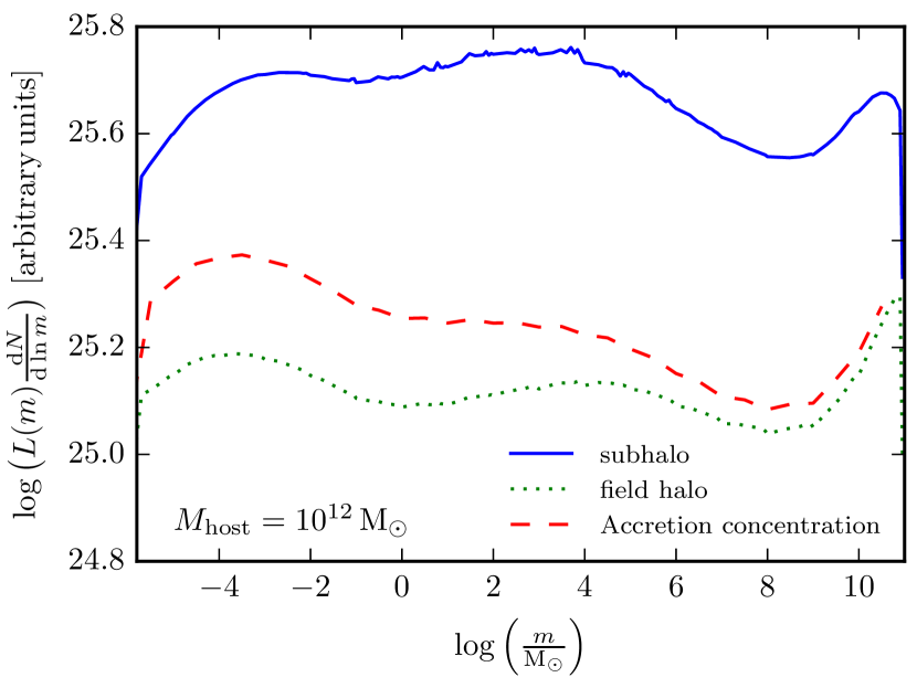
Figure 1: Luminosity-weighted mass function for subhalos (solid), field halos whose concentration is set at $z=0$ (dotted) and field halos which have the same infall times as the solid line (dashed) in a $10^{12}\mathrm{\,M_{\odot}}$ host. It shows the contribution of different mass subhalos to the overall subhalo luminosity. We always use the subhalo mass function from Table 1.

V.1 Boost ratio

It is interesting to compare luminosities of subhalos obtained above with those of field halos of equal mass. We assume field halos to be virialized at $z=0$ with $r_{\mathrm{vir}}$ given by $m=4\pi\Delta_{\rm c,0}\rho_{\rm c,0}r_{\mathrm{vir}}^{3}/3$. The characteristic density and scale radius are again obtained with $r_{\rm s,fh}=r_{\mathrm{vir}}/c_{\mathrm{vir}}(m,0)$ and $\rho_{\rm s,fh}=m_{\mathrm{vir}}/[4\pi r_{\mathrm{s}}^{3}f(c_{\mathrm{vir}}(m,0))]$, where the concentration mass relation of Ref. Correa et al. (2015) is assumed. Then the field halo luminosity is, $L_{\rm fh}(m)\propto\rho_{\mathrm{s}}^{2}r_{\mathrm{s}}^{3}[1-1/(1+c_{\mathrm{vir}})^{3}]$. The dotted curve in Fig. 1 shows the luminosities $L_{\rm fh}(m)$ weighted by the same mass function as in the case of $L_{\rm sh}(m)$. As anticipated above, the field halos are less bright than the subhalos of the same mass by a factor of a few, almost independent of mass $m$.

It should be noted that subhalo concentrations depend on formation time. Halos that formed earlier are more concentrated since they formed in a denser background, an effect that has been taken into account in past studies (e.g., Refs. Pieri et al. (2008); Kamionkowski et al. (2010); Ng et al. (2014)). Since we set the concentration of the stripped halos at $z_{\mathrm{a}}$ we also include the dashed line for a fully fair comparison. It shows the luminosity of halos that follow the same infall distribution as the solid line, and thus have the same natal concentration as this is set at the time of accretion, but are not tidally stripped. As can be seen, the tidal stripping still yields an increase by a factor of $\sim$2 at any subhalo mass. The decrease in the difference in luminosity at lower masses is due to the smallest halos being accreted earlier, thus their concentrations at accretion differ most compared to that at $z=0$.

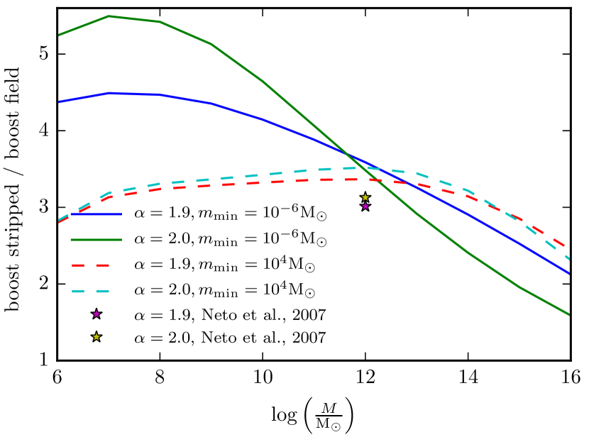
Figure 2: Boost using stripped-subhalo luminosities over that from field-halo luminosities. Four fiducial models of the subhalo mass function are adopted, with minimum subhalo masses of $m_{\mathrm{min}}=10^{-6}\mathrm{\,M_{\odot}}$ and $10^{4}\mathrm{\,M_{\odot}}$ and slopes $\alpha=1.9$ and 2. Starred symbols show results using the concentration-mass relation from Ref. Neto et al. (2007), assuming $m_{\mathrm{min}}=10^{4}\mathrm{\,M_{\odot}}$ and $c_{\mathrm{vir}}(z|m)\propto z^{-0.5}$.

Since the boost depends critically on the subhalo mass function, in addition to our fully self-consistent model with the mass-function from Table 1, we also investigate dependence on several models for the mass function. We adopt four models, taking spectral indices of $\alpha=1.9$ and 2, and smallest subhalo masses of $m_{\mathrm{min}}=10^{-6}\,{\rm M}_{\odot}$ and $10^{4}\,{\rm M}_{\odot}$. We compare the subhalo boost $B_{\rm sh}(M)$, calculated with Eq. (1), using subhalo luminosities of stripped halos, to the boost calculated without accounting for tidal effects (using the virialized field halo models). Figure 2 shows the ratio of boosts as a function of host halo mass for these models. Taking tidal effects into account will enhance the boost by up to a factor of 5 compared to the simple field halo approach, consistently for host halo masses between $10^{6}$–$10^{15}\,{\rm M}_{\odot}$. This is largely independent of models of the subhalo mass function.

Next to the results obtained using the concentration-mass relation of Ref. Correa et al. (2015) (shown as solid and dashed curves in Fig. 2), we also show results for Milky-Way-sized halos when using the concentration-mass relation from Ref. Neto et al. (2007) assuming $m_{\mathrm{min}}=10^{4}\,\mathrm{M_{\odot}}$ and $c_{\mathrm{vir}}(z|m)\propto z^{-0.5}$ as starr1ed symbols. Both concentration models agree well for large mass halos, but differ significantly for smaller masses, closer to the resolution of the current-generation simulations, $10^{5}\,{\rm M}_{\odot}$. However, our results show that the boost ratio is insensitive to the initial choice of the concentration-mass relation. We also see that our semi-analytic model provides relatively smaller boost ratios compared with what is inferred from simulations directly Springel et al. (2008b), as estimated above. It might be an indication that our approach provides a more conservative boost relative to the dark-matter-only simulations, even though an increase in boost by upto a factor of $\sim$4 for the Milky-Way-sized halo is substantial.

V.2 Boost

Figure 3 shows the overall boost factor using the subhalo mass functions that came out of our analysis (Table 1), as well as a few other phenomenological models of mass functions. For all cases we adopt the luminosities for stripped subhalos (solid lines), and compare to the luminosity using the ordinary field-halo approach (dotted). We caution that this boost can only be compared to other boost factors presented in the literature when taking the differences in the subhalo mass functions and concentration-mass relations properly into account. For example our boosts (solid lines in Fig. 3) are comparable to those of Ref. Sanchez-Conde and Prada (2014) where the tidal effect was not included. This is because our model is based on the concentration-mass relation from Ref. Correa et al. (2015), which yields an even more modest boost and cancels the enhancement due to inclusion of the tidal effect. To be explicit, if we instead ran our analysis with the concentration-mass relation from Ref. Sanchez-Conde and Prada (2014), we would have found a boost that is 2–5 times larger than theirs. Similar arguments hold for different concentrations (including a simple power law).

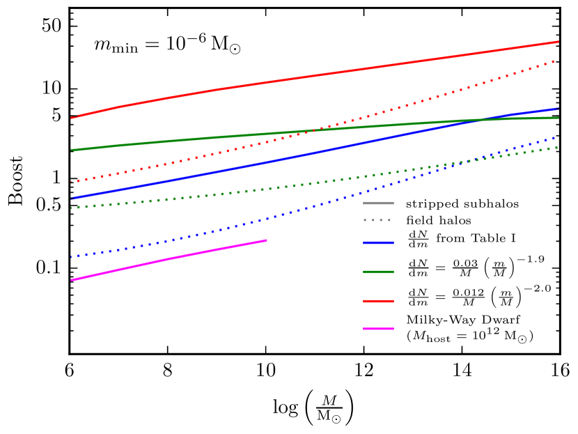
Figure 3: Boost factors for halos of different mass using the concentration-mass relation from Ref. Correa et al. (2015). Solid curves include the effect of tidal stripping, dotted curves assume field halo concentrations. The boost for three different subhalo mass functions are shown, using those from Table 1 (blue) and Ref. Sanchez-Conde and Prada (2014) (green and red). The expected boost for dwarf satellites of the Milky Way, adopting the mass functions from Table 1 is also shown (magenta).

Estimate for dwarf spheroidal galaxies

We estimate the expected boost for Milky-Way satellite galaxies. The density profile of the dwarf galaxies is taken to be that of a subhalo of given mass in a $10^{12}\mathrm{\,M_{\odot}}$ host. Therefore, the smooth component of the dwarf has a higher luminosity than that of similar-mass halos in the field. By de-projecting the surface brightness from substructures Gao et al. (2012); Han et al. (2012); Ando and Komatsu (2013), we estimate that about two thirds of the sub-subhalos lies outside of the tidal radius and is stripped away. This simple rescaling of the substructure mass function agrees with what is done by Refs. (Diemand et al., 2008; Kuhlen et al., 2008). However, this method likely yields an upper limit to the amount of sub-substructure, since, whereas sub-subhalos lose mass due to tidal effects, no additional sub-subhalos fall into the subhalo anymore (Springel et al., 2008b). The combined effect of the satellite being brighter than similar-mass field halos and the loss of sub-substructure makes the boost of satellite galaxies one order of magnitude smaller compared to their companions in the field. This supports the usual assumption that the boost due to sub-substructure is negligible. Nevertheless, we show an estimate of how sub-substructure impacts our results in Fig. 3. For this estimate we assumed that two-thirds of the sub-substructure gets stripped away and that $L_{\mathrm{ssh}}(m)=L_{\mathrm{sh}}(m)$. We explicitly checked this at all host halo masses considered and the sub-substructure contribution is never more than $\sim$10%.

VI Discussion

We find that consistently modeling the subhalo luminosity by taking into account tidal effects significantly enhances the global boost factor, compared to orthodox use of the concentration-mass relation. This result is independent of uncertainties in the subhalo mass function or concentration-mass relation.

Thus far, we applied a dark-matter only analysis, but state-of-the-art numerical simulations study the effects of baryons. Although they can change subhalo abundance and density profile, we do not expect them to have major impact on our results. First, the concentration-mass relations remain similar Sawala et al. (2015); Schaller et al. (2014). Second, low-mass ($\lesssim 10^{8}$–$10^{9}\mathrm{\,M_{\odot}}$) halos, which give major contribution to the boost (Fig. 1), are not expected to have a large baryonic component in them. Nevertheless, we took a conservative approach by estimating the boost ratio assuming that baryons would undo the effect of stripping completely in subhalos $\leq 10^{8}\mathrm{\,M_{\odot}}$, and in the scenario where this has most impact ($m_{\mathrm{min}}=10^{4}\mathrm{\,M_{\odot}}$, and $\alpha=1.9$), the decrease is at most $\sim$30%.

Encounters of subhalos with stars in the disk of the host will disrupt subhalos (e.g., Refs. Green and Goodwin (2007); Goerdt et al. (2007)). However, this happens only in a small volume close the halo center, and thus, will not affect the conclusions either.

This study will have a broad impact on indirect dark matter searches in the extragalactic gamma-ray sky. Recent developments include the updated analysis of constraints on annihilation cross section from the diffuse gamma-ray background Ackermann et al. (2015), its anisotropies Ando and Komatsu (2013); Gomez-Vargas et al. (2014), and cross correlations with dark matter tracers Ando et al. (2014); Fornengo and Regis (2014); Ando (2014); Regis et al. (2015). All these probes are subject to uncertainties in the halo substructure boost. Our conclusions are promising because having the boost factor larger by a factor of 2–5 enhances the detectability (or improves the present upper limits) by the same factor.

appendix

First, we provide some details on the $V_{\mathrm{max}}$–$r_{\mathrm{max}}$ relation we find in our analysis and show that it is consistent with the one obtained with numerical simulations. Next, we have an extended discussion on the use of an Einasto profile rather than NFW. We repeat the order-of-magnitude estimate for the luminosity ratio in this context. Finally, we show how the boost depends on the minimum subhalo mass.

A $V_{\mathrm{max}}$–$r_{\mathrm{max}}$ relation

In addition to the above analysis in terms of the evolution of the concentration parameters, we discuss our results in terms of the $V_{\mathrm{max}}$–$r_{\mathrm{max}}$ relation, whose evolution we modelled following Refs. Penarrubia et al. (2008); *Penarrubia:2010jk as described above.

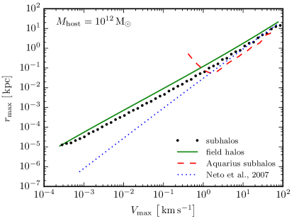
Figure A-4: $V_{\mathrm{max}}$-$r_{\mathrm{max}}$ resulting from our analysis (dots) compared to that of field halos with the concentration of Ref. Correa et al. (2015) (green solid). The relation for field halos with the concentration of Ref. Neto et al. (2007) (blue dotted) and the results from the Aquarius simulation(Springel et al., 2008b) (red dashed) are also shown for comparison.

For subhalos in the Milky-Way-sized host, we compare the $V_{\mathrm{max}}$–$r_{\mathrm{max}}$ resulting from our analysis to that of field halos with the concentration of Ref. Correa et al. (2015). Like the simulation results (Springel et al., 2008b; Hellwing et al., 2015), we find that for the same $V_{\mathrm{max}}$, subhalos have a smaller $r_{\mathrm{max}}$ compared to field halos by a factor $\sim$0.6. However, we find a softer slope ($\sim$1.13–1.15), which is a consequence of our choice for the concentration mass relation. Across seventeen orders of magnitude, we find $(r_{\rm max,sh}/r_{\rm max,fh})\approx 0.6(V_{\rm max,sh}/V_{\rm max,fh})^{1.1}$ and $m_{\mathrm{sh}}\approx 6.2\times 10^{7}(V_{\rm max,sh}/10\mathrm{\,km\,s^{-1}})^{3.2}\mathrm{\,M_{\odot}}$ to hold, leading to $L_{\rm sh}/L_{\rm fh}\approx 4$. The $V_{\mathrm{max}}$–$r_{\mathrm{max}}$ relation for our subhalos is plotted in Fig. A-4. We also plot the relation for subhalos that is found in the Aquarius simulation Springel et al. (2008b). In addition, we show what is deduced for field halos when using the mass-concentration relation from Ref. Neto et al. (2007). By running the analysis with this concentration-mass relation instead, we find a relation with a steeper slope that is consistent with the findings of the simulations Springel et al. (2008b). Concretely, we then find $(r_{\rm max,sh}/r_{\rm max,fh})\approx 0.5(V_{\rm max,sh}/V_{\rm max,fh})^{1.5}$ and $m_{\mathrm{sh}}\approx 4.9\times 10^{7}(V_{\rm max,sh}/10\mathrm{\,km\,s^{-1}})^{3.4}\mathrm{\,M_{\odot}}$

B Einasto Profile

$V_{\mathrm{max}}$ and $r_{\mathrm{max}}$ are measurable quantities in the numerical simulations, and unlike the NFW scale radius and density, they are not profile dependent. However, in the above analysis we explicitly calculated $V_{\mathrm{max}}$ and $r_{\mathrm{max}}$ starting from the assumption of an NFW profile for field and subhalos, and thereby we introduced a bias. Unfortunately, in our semi-analytic framework we are forced to resort to halo density profiles, only in simulations one is able to compare the $V_{\mathrm{max}}$–$r_{\mathrm{max}}$ relation independently of the profile (Springel et al., 2008b).

The fact that our results resemble what is observed in simulations (Fig. A-4) is encouraging. Nevertheless, we here also discuss what happens when applying an Einasto profile (Graham et al., 2006a, b):

$$\rho_{\mathrm{Ein}}(r)=\rho_{\mathrm{s,Ein}}\exp\left(-\frac{2}{\alpha}\left[\left(\frac{r}{r_{\mathrm{s,Ein}}}\right)^{\alpha}-1\right]\right).$$ (7)

Reference Klypin et al. (2014) points out that, especially at large halo masses ($\gtrsim 10^{14}\mathrm{\,M_{\odot}}$), the Einasto profile performs better than the NFW in fitting simulated halos.

Below we will perform an order of magnitude estimate similar to that in main text, but now for an Einasto profile. In what remains we will closely follow the approach for calculating halo concentrations for Einasto profiles as laid out in Ref. (Klypin et al., 2014). First, we define the concentration for the field halos with the Einasto profile as $c_{\mathrm{Ein}}\equiv{r_{\mathrm{vir}}}/{r_{\mathrm{s,Ein}}}$. Starting from a concentration-mass relations for NFW halos, $c_{\rm Ein}$ can be obtained by requiring either that $r_{\mathrm{max,\,NFW}}=r_{\mathrm{max,\,Ein}}$ or $V_{\mathrm{max,\,NFW}}=V_{\mathrm{max,\,Ein}}$. We will use the former. Since these are physical quantities, they should in principle be the same. However, we systematically deviate from the real $V_{\mathrm{max}}$ and $r_{\mathrm{max}}$ because we assume some density profile. As a result, by fixing $r_{\mathrm{max,\,NFW}}=r_{\mathrm{max,\,Ein}}$ we in general will obtain $V_{\mathrm{max,\,NFW}}\neq V_{\mathrm{max,\,Ein}}$. In this case we obtain

$$c_{\rm Ein}\approx c_{\rm NFW}\frac{3.15\exp\left(-0.64\alpha^{1/3}\right)}{2.163},$$ (8)

where we used $r_{\mathrm{max,\,Ein}}\approx 3.15\exp\left(-0.64\alpha^{1/3}\right)r_{\mathrm{s,Ein}}$ (Klypin et al., 2014). We obtain $\alpha$ from Eq. (23) in Ref. Klypin et al. (2014), which expresses $\alpha$ in terms of $\nu$, the peak height in the linear density fluctuation field.

With this in place, we can now calculate the luminosity ratio as in the order-of-magnitude estimate in the main text. We again apply the concentration-mass relations from Ref. (Neto et al., 2007) and use the phenomenological relations from Ref.  Springel et al. (2008b), which we repeat here: $(r_{\rm max,sh}/r_{\rm max,fh})\approx 0.62(V_{\rm max,sh}/V_{\rm max,fh})^{1.49}$ and $m_{\mathrm{sh}}\approx 3.37\times 10^{7}(V_{\rm max,sh}/10\mathrm{\,km\,s^{-1}})^{3.49}\mathrm{\,M_{\odot}}$. We find $c_{\rm Ein}\approx 107$ and $V_{\rm max,Ein}\approx 1.3\mathrm{\,km\,s^{-1}}$ for $m_{\rm fh}=10^{5}$. Finally, for the subhalos and field halos of equal mass with the Einasto profile, the relation, $L_{\rm sh}/L_{\rm fh}\approx(\rho_{\rm s,sh}/\rho_{\rm s,fh})^{2}(r_{\rm s,sh}/r_{\rm s,fh})^{3}=(V_{\rm max,sh}/V_{\rm max,fh})^{4}(r_{\rm max,fh}/r_{\rm max,sh})$, still holds. Note that the last equality is only exact if the field and subhalo have identical $\alpha$’s. This yields $L_{\rm sh}/L_{\rm fh}\approx 4$ for $m_{\rm sh}=10^{5}\,{\rm M}_{\odot}$ and $L_{\rm sh}/L_{\rm fh}\approx 3$ for $m_{\rm sh}=10^{9}\,{\rm M}_{\odot}$.

The above results are slightly lower than what we obtained when assuming an NFW profile. It can be understood by the fact that at higher masses $V_{\mathrm{max,\,NFW}}<V_{\mathrm{max,\,Ein}}$, when assuming $r_{\mathrm{max,\,NFW}}=r_{\mathrm{max,\,Ein}}$. This makes field halos with an Einasto profile brighter than those with an NFW profile. However, most importantly, a change in profile does not alter our qualitative conclusions about the effect of tidal stripping on the subhalo luminosity.

C Boost dependence on mass of the smallest subhalos

Finally, in Fig. A-5 we show how the boost depends on the minimal subhalo mass in a MW-sized host. We show the boost for stripped subhalos (solid) and compare it to the field-halo approach (dotted) and again the concentration-mass relation is from Ref. Correa et al. (2015). This relation flattens at lower masses. We also show the power-law extrapolation from the Aquarius simulation (Springel et al., 2008a). This is equivalent to a power-law concentration-mass relation.

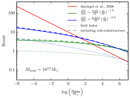
Figure A-5: The boost as a function of the minimum subhalo mass in a Milky-Way-sized host halo, for stripped subhalos (solid and dashed) and field-halo concentrations (dotted). The concentration-mass relation is from Ref. Correa et al. (2015), and flattens towards lower masses. We also show the power-law extrapolation of the Aquarius results Springel et al. (2008a) (red).