1 Introduction

In this paper we consider robust models for emergency staff deployment in the event of a flu pandemic. We focus on managing critical staff levels at organizations that must remain operational during such an event, and develop methodologies for managing emergency resources with the goal of minimizing the impact of the pandemic. We present numerical experiments using realistic data to study the effectiveness of our approach.

A serious flu epidemic or pandemic, particularly one characterized by high contagion rate, would have extremely damaging impact on a large, dense population center. The 1918 influenza pandemic is often seen as a worst-case scenario as it arguably represents the most devastating pandemic in recent history, having killed more than 20 million people worldwide [10, 38, 48]. However, even a much milder epidemic would have vast social impact as services such as health care, police and utilities became severely hampered by staff shortages. Workplace absenteeism might also become a serious concern [49]; for example, the New Zealand government has predicted overall absenteeism levels as high as 40% ([34] and references therein)

In this study we focus on managing the inevitable staff shortfall that will take place in the case of a severe epidemic. We take the viewpoint of an organization that seeks to diminish decreased performance in its operations as the epidemic unfolds, by appropriately deploying available resources, but which is not directly attempting to control the number of people that become infected. In contrast to our focus, much valuable research has been directed at addressing the epidemic itself; such work studies public health measures that would reduce the epidemic’s severity and its direct impact, for example by managing the supply of vaccines and antivirals (see [35, 28, 36]). While we do not address this topic, it seems plausible that our methodology for handling robustness will apply in this setting, as well.

We are interested in infrastructure of critical social value, such as hospitals, police departments, power plants and supply chains, among many examples of entities that must remain operative even as staff levels become low. In cases such as police departments, staff would likely be more exposed to the epidemic than the general public and (particularly if vaccines are in short supply, or apply to the wrong virus mutation) shortfalls may take place just when there is greatest demand for services. Power plants and waste water treatment plants are examples of facilities whose operation will be degraded as staff falls short and which probably require minimum staff levels to operate at all [29]. Supply chains would very likely be significantly slowed down as their staff is depleted, resulting, for example, in food shortages [43]. In all these cases, organizations cannot implement “work from home” strategies as urged for private businesses by the Centers of Disease Control and Prevention (CDC) and the United States Department of Labor .

A pandemic contingency plan for a large organization (such as a city government) would include resorting to emergency (or “surge”) sources for additional staff: for example by temporarily relying on personnel from outlying, less dense, communities. Such additional resources are likely to be significantly constrained in quantity, duration and rate, among other factors. Such emergency staff deployment plans would entail some complexity in design, calibration and implementation, but as a result of other disasters such, as Hurricane Katrina in 2005 and the anthrax attacks in 2001, it is now agreed that there is a compelling need for emergency planning [20].

From a planner’s perspective, the task of managing future resource levels during an epidemic is complex, partly because of uncertainties regarding the behavior of the epidemic, in particular, uncertainty in the contagion rate. The evolution of the contagion rate is a function of poorly understood dynamics in the mutations of the different strains of the flu virus and environmental agents such as weather [10, 37]. In addition to uncertainty, a decision-maker will also likely be constrained by logistics. In particular, it may prove impossible to carry out large changes to staff deployment plans on short notice, particularly if such staff is also in demand by other organizations (as might be the case during a severe epidemic). We will return to these issues in Sections 6.2 and 8. As a consequence of the two factors (uncertainty, and logistical constraints) a decision-maker may commit too few or too many resources - in this case emergency staff- or perhaps at the wrong time, if there turns out to be a mismatch between the anticipated level of staff shortage and what actually transpires (after the resources have been committed).

We present models and methodology for developing emergency staff deployment levels which optimally hedge against the uncertainty in the evolution an the epidemic while accounting for operational constraints. Our approach overlays adversarial models to describe the contagion rate on the classical SEIR model for describing epidemics. The resulting robust optimization models are nonconvex and large-scale; we present convex approximations and algorithms that prove numerically accurate and efficient, and we study their behavior and the policies they produce under a range of scenarios.

This paper is organized as follows. Section 2 addresses issues related to surge capacity planning; Section 3 describes the classical (non-robust) SEIR model; Sections 5, 4 and 6 contain the description of our initial robust model, Section 7 describes our experiments, and our algorithms are detailed in Appendix A.

2 Planning for workforce shortfall

An influenza pandemic would severely stress the operational continuity of social and business structures through staff shortages. Staff shortfall directly resulting from individuals becoming sick could be intensified by policy or absenteeism. For example, during the last H1N1 influenza outbreak, CDC recommended that people with influenza-like symptoms remain at home until at least 24 hours after they are or appear to be free of fever. In the particular case of health care workers it is advised that they refrain from work for at least 7 days after symptoms first appear (see [17] for additional details). Moreover, staff shortages may occur not only due to actual illness, but also from illness among family members, quarantines, school closures (combined with lack of child care), public transportation disruptions, low morale, or because workers could be summoned to comply with public service obligations [49, 21]. Indeed, employees who have been exposed to the disease (especially those coming into contact with an ill person at home) may also be asked to stay at home and monitor their own symptoms.

Altogether, the direct and indirect staff shortfall caused by an epidemic, in a worst-case scenario, could give rise to an extended time period during which 20 to 40% of the workforce will be absent, public health and utility professionals predict [29]. Even though the outlook would be dire, organizations that provide critical infrastructure services such as health care, utilities, transportation, and telecommunications, should clearly continue operations and are exhorted to plan accordingly [42]. (See [39] for additional background on emergency staff planning.)

The Department of Health and Human Services (HHS) and the CDC have provided guidelines to help businesses and their employees in planning for an influenza outbreak. In addition to recommendations addressing the spread of disease and antiviral drug stockpiling, there is a focus on staff planning, which is the subject of our study [42, 17]. Additionally, there are federal and state programs such as the New York Medical Reserve Corps whose mission is to organize volunteer networks prepare for and respond to public health emergencies, among other duties [11].

HHS and CDC urge organizations to identify critical staff requirements needed to maintain operations during a pandemic. In particular, organizations should develop detailed criteria to determine when to trigger the implementation of an emergency staffing plan. Most significantly, organizations should identify the minimum number of staff needed to perform vital operations. For example, in the case of water treatment plants, approximately 90% of the personnel is critical for keeping the utility running; for refineries, losing 30% of their staff would force a shutdown [29].

In the particular case of hospitals, an effective contingency staffing plan should incorporate information from health departments and emergency management authorities at all levels, and would build a data base for alternative staffing sources (e.g., medical students). For additional details, see [42, 27]. In New York City, for example, after the events of 9/11, Columbia University created a database of volunteers to be recruited and trained both in basic emergency preparedness and their disaster functional roles [39]. At the city level the NYC Medical Reserve Corps ensures that a group of health professionals ranging from physicians to social workers is ready to respond to health emergencies. The group is pre-identified, pre-credentialed, and pre-trained to be better prepared in the wake of a crisis. Similar emergency staff backup plans could be implemented in all other cases of utilities and social infrastructure [11].

In spite of all these efforts, it seems clear that much remains to be done and that a severe epidemic would place extreme strain on infrastructure. A good example is provided by the 2009 Swine Flu epidemic. Even though the virus mutation caused few fatalities, and a successful vaccine became available, New York hospitals were severely stressed [50]: “The outbreak highlighted many national weaknesses: old, slow vaccine technology; too much reliance on foreign vaccine factories; some major hospitals pushed to their limits by a relatively mild epidemic” (our emphasis).

From our perspective, the uncertainty concerning the timeline and severity of the pandemic brings substantial complexity to the problem of deploying replacement staff. This problem, which will be the core issue that we address, is relevant because significant preplanning must take place and it is unlikely that major quantities of additional workforce can be summoned on a day-by-day basis.

2.1 Declaring an epidemic

A technical point that we will return to below concerns when, precisely, an epidemic is “declared”. In the case of an infectious disease such as influenza, an initially slow accumulation of cases followed by a more rapid increase in incidence [24] is viewed by epidemiologists as an epidemic. However, this definition is too general for planning purposes. This is a significant issue since emergency action plans would be activated when the epidemic is declared.

In the United States, the CDC declares an influenza epidemic when death rates from pneumonia and influenza exceed a certain threshold [16]. Each week, vital statistics of 122 cities report the total number of death certificates received and the proportion of which are listed to be due to pneumonia or influenza. This percentage is compared against a seasonal baseline, which in turn was computed using a regression model based on historic data. There is a different baseline for each week of the year to capture the different seasonal patterns of influenza-like illnesses (ILI) (the epidemic threshold sits 1.645 standard deviations above the seasonal baseline). This type of measure is not specific for the United States. In [34], the authors’ base case assumed that the duration of an influenza pandemic in Singapore was defined as the period during which incident symptomatic cases exceeded 10% of baseline ILI cases.

Motivated by this discussion, we will use the convention that an epidemic is known to be present as soon as the number of (new) infected individuals on a given time period exceeds a small percentage of the overall population, e.g. $0.93\%$, which corresponds to the national epidemic threshold of $6.5\%$ for week $40$[16].

From the point of view of an organization, of course, action need not wait until an “official” epidemic declaration and would instead rely on its own guidelines to possibly implement a preparedness plan at an earlier point. However, we expect that the mechanism underlying declaration will be the similar.

3 Modeling influenza

Influenza is an acute, highly contagious respiratory disease caused by a number of different virus strains. While most people recover within one or two weeks without requiring medical treatment, influenza may cause lethal complications such as pneumonia. For certain virus strains this is especially pronounced in the case of susceptible groups such as young children, the elderly or people with certain medical preconditions.

Yearly influenza outbreaks occur because the different virus strains acquire adaptive immunity to old vaccines by frequent mutations of their genetic content [14]. According to the CDC, seasonal influenza causes an average of 23,600 deaths and more than 200,000 hospitalizations in the U.S. [42]. When a larger genomic mutation occurs the virus derives into a new one for which humans have little or no immunity resulting in a pandemic: the disease may rapidly spread worldwide, possibly with high mortality rates.

There were three flu pandemics in the twentieth century, the worst of which occurred in 1918; known as the “Spanish flu”, it killed 20-40 million people worldwide. Milder pandemics occurred in 1957 and 1968. The most recent pandemic occurred in 2009 - 2010 with the surge of the H1N1 virus. Current fears that the avian strain could develop into another pandemic have caused interest in modeling the spread of influenza and evaluating possible emergency management strategies.

The critical difficulty in modeling the impact of a future influenza pandemic is our inability to accurately predict the spread of disease on a given population. In this section we provide a description of the (nonrobust) model which we will modify in order to follow the evolution of the disease and its spread among members of a given population. We focus on the progress of the epidemic within a workforce group of interest. We then discuss weaknesses of the model and the use of robust methods to remedy these shortcomings.

3.1 SEIR – a basic influenza model

A classic simple model for influenza is the so called $SEIR$ compartmental model. These kind of models describe, in a deterministic fashion, the evolution of the disease by partitioning the population into groups according to the progression of the disease. The terminology $SEIR$ describes the transition of individuals between compartments: from susceptible ($S$) to being in an incubation period ($E$) to becoming infectious ($I$) and finally to the removed class ($R$). The latter could include death due to infection as well as recovered people, depending on the model.

We make the following standard assumptions [7]:

1. There is a small number $I_{0}$ of initial infectives relative to the size of the total population, which we denote by $N$.

2. The rate at which individuals become infected is given by the product of the probability that at time $t$ a contact is made with an infectious person, $\beta_{t}$, the average constant social contact rate $\lambda$, and the likelihood of infection, $p$, given that a social contact with an infectious person has taken place. The probability $\beta_{t}$ changes with time because we assume it depends on the number of infectious agents in the population.

3. The latent period coincides with the incubation period; that is, exposed individuals are not infectious. We assume they proceed to the $I$ compartment with rate $\mu_{E}$.

4. Infectives leave the infectious compartment at rate $\mu_{RR}$.

5. We assume there is only one epidemic wave. Thus, people who recover are conferred immunity.

6. The fraction of members that do not die from the disease, when removed from the infectious class, is given by $0\leq f<1$.

7. We do not include births and natural deaths because influenza epidemics usually last few months. We also omit any migration. In other words, excluding deaths by disease, the total population remains constant.

SEIR models are usually described as a system of nonlinear ordinary differential equations (see for example [7, 41]). For our purposes, we use a discrete-time Markov chain type approximation along the lines of [33] and similar to those found in [2, 3, 4]:

$$S_{t+1} = S_{t}(e^{-\lambda\beta_{t}p})$$

$$E_{t+1} = E_{t}(e^{-\mu_{E}})+S_{t}(1-e^{-\lambda\beta_{t}p})$$ (1)

$$I_{t+1} = I_{t}f(e^{-\mu_{RR}})+E_{t}(1-e^{-\mu_{E}})$$

$$R_{t+1} = R_{t}+I_{t}(1-e^{-\mu_{RR}}).$$

Compartmental models incorporate a number of assumptions to describe social contact dynamics. First, the number of social contacts with infectious people for an arbitrary person is thought of as a Poisson random variable with rate $\lambda\beta_{t}$; we use one day as time unit. Second, the models assume homogeneous mixing, that is, all individuals have a fixed average number of contact rates per unit of time and are all equally likely to meet each other. Thus, the probability that a contact is made with an infectious person, $\beta_{t}$ is given by $I_{t}/N$. The daily infectious contact rate $\lambda p$ is usually written as $\lambda$ [7, 3] and taken as a constant throughout the epidemic. We will remove this assumption later when we make the transmissibility parameter $p$ explicit.

If the number of initial infectives is relatively very small compared to the whole population ($S_{0}\sim N$), then a newly introduced contagious individual is expected to infect people at the rate $\lambda p$ during the expected infectious period $1/\mu_{RR}$. Thus, each initial infective individual is expected to transmit the disease to an average of

$$R_{0}=\frac{\lambda\,p}{\mu_{RR}}$$ (2)

individuals. $R_{0}$ is called the basic reproduction number (also known as basic reproduction ratio or basic reproductive rate.) It is without doubt the most important quantity epidemiologists consider when analyzing the behavior of infectious diseases [7]. Its relevance derives mainly from its threshold property: when $R_{0}<1,$ the disease does not spread fast enough and there is no epidemic; when an epidemic does take place, it is of interest to see how much bigger than 1 $R_{0}$ is. Because we assume that an epidemic will take place a priori, $R_{0}$ is not of particular interest to us; however, it is presented here for completeness.

3.1.1 Keeping track of staff availability

We are interested in tracking workforce availability at a particular organization during the epidemic; following previous work [5, 19] we divide the population into two groups: (1) the general population and (2) the workforce under consideration. Individuals from the latter group could have a very different exposure to the epidemic. For example, people working at a water plant could have lower contact rates than average (by virtue of having contact with few individuals during the workday) while the staff at a health clinic may not only have higher contact rates, but may also have easier access to antiviral medicines that reduce their infectiousness and the length of the infectious period.

For ease of notation, we use superscript $1$ to refer to the general population and $2$ to refer to the group of workers of interest. For $j=1,2$, define compartments $S^{j},E^{j},I^{j},R^{j}$ corresponding to group $j$. Following the discussion above, we allow the groups to have different contact, incubation, and recovery rates. The probability that a random contact is one with an infected person at time $t$, $\beta_{t}$, is now defined as

$$\beta_{t}=\frac{\lambda^{T}I_{t}}{\lambda^{T}N_{t}},$$ (3)

where $I_{t}=[I^{1}_{t},I^{2}_{t}]$ is the vector of infectious individuals at time $t$, $\lambda^{T}=[\lambda^{1},\lambda^{2}]$ is the vector of contact rates, and $N_{t}=[N_{t}^{1},N_{t}^{2}]$ denotes the size of each group at time $t$. We note that $\beta_{t}$ is constant across groups. We now have two parallel thinned Poisson process approximations, each with rate $(\lambda_{j}\beta_{t}p)$. The set of equations that correspond to group $j$ ($=1,2$) is

$$S^{j}_{t+1} = S^{j}_{t}e^{-\lambda_{j}\beta_{t}p}$$

$$E^{j}_{t+1} = E^{j}_{t}e^{-\mu_{E}}+S^{j}_{t}(1-e^{-\lambda_{j}\beta_{t}p})$$ (4)

$$I^{j}_{t+1} = I^{j}_{t}fe^{-\mu_{RR}}+E^{j}_{t}(1-e^{-\mu_{E}})$$

$$R^{j}_{t+1} = R^{j}_{t}+I^{j}_{t}(1-e^{-\mu_{RR}}).$$

We now give an expression for $R_{0}$ [7, 13]. First we note that the average contact rate for subgroup $j$ at time $0$ is given by

$$\frac{\lambda_{j}N^{j}}{\lambda_{1}N^{1}+\lambda_{2}N^{2}}.$$

Thus, the average number of new infections caused by a newly infective person introduced into an otherwise susceptible population is given by

$$R_{0} =\left[\lambda_{1}\frac{\lambda_{1}N^{1}}{\lambda_{1}N^{1}+\lambda_{2}N^{2}}+\lambda_{2}\frac{\lambda_{2}N^{2}}{\lambda_{1}N^{1}+\lambda_{2}N^{2}}\right]\frac{p}{\mu_{RR}}$$

$$=\frac{\lambda_{1}^{2}N^{1}+\lambda_{2}^{2}N^{2}}{\lambda_{1}N^{1}+\lambda_{2}N^{2}}\cdot\frac{p}{\mu_{RR}}.$$ (5)

We note that when $\lambda_{1}=\lambda_{2}$ (5) reduces to (2).

3.1.2 Nonhomogeneous mixing and social distancing

We initially assumed that the population mixed homogeneously, that is the contact rates $\lambda_{1}$ and $\lambda_{2}$ remained constant throughout. However, the homogeneous mixing and mass action incidence assumptions have clear pitfalls; individuals from each compartment are hardly indistinguishable in terms of their social patterns and likeliness of infection. As more people acquires the disease, members in the population may become more careful of their social contacts and infectious people may stay at home. Thus, following [3] we make the assumption that

$$\lambda^{j}_{t}=\Lambda_{j}\frac{S^{j}_{t}+E^{j}_{t}+R^{j}_{t}}{N^{j}_{t}},\quad j=1,2,$$ (6)

where $\Lambda_{j}$ are fixed constants, $j=1,2.$ Using this definition, $\lambda^{j}_{t}$ decreases whenever there is a high number of infectious agents in the population. As mentioned in [3], other functional forms are possible; we rely on (6) because it provides a simple way to capture changes in contact rates as a function of severity of the epidemic.

Additionally, we also consider a scenario in which authorities impose social distancing measures as soon as the epidemic is declared. A similar situation took place in Mexico during the last 2009 H1N1 epidemic, where venues such as schools, movie theaters, and restaurants were forced to close temporarily. It is estimated that the transmission of the disease was diminished by $29$% to $37$% [9]. We incorporate this element by multiplying the contact rates by an additional dampening factor when the epidemic is considered declared and until the rate of growth of daily infectives is below some threshold (we refer the reader to section 2.1). Effectively, the contact rate for group $j$ at time $t$ becomes $\lambda^{j}_{t}=\theta\Lambda_{j}\left(\frac{S^{j}_{t}+E^{j}_{t}+R^{j}_{t}}{N^{j}_{t}}\right)$ ($0<\theta<1$) when the epidemic is officially ongoing; otherwise, it remains as per equation (6).

4 Robustness in planning

In planning the response to a future or impending epidemic, one would need to rely at least partly on an epidemiological model, and such a model would have to undergo careful calibration in order to be put to practical use. This is especially the case for the SEIR model presented above, which is rich in parameters that need to be estimated to fully define the trajectory of the epidemic. In the case of a flu pandemic caused by an unknown virus strain, new parameter values would need to be promptly estimated as the epidemic emerges. Ideally, robust statistical inference would provide information on all parameters, though data paucity would present a challenge.

On the positive side, the infectious and incubation periods can usually be independently estimated via clinical monitoring of infected agents, either by observation of transmission events or by the use of more detailed techniques [31].

On the other hand, it is not clear how to accurately estimate the transmission rate $\lambda_{j}p$. One approach is to approximate the basic reproductive ratio $R_{0}$ and the mean infectious period, and then use equation (2). There are multiple ways of estimating $R_{0}$; see, for example, [10]. Given that the definition of $R_{0}$ is based on the early stages of the epidemic, one should examine its early behavior. However, the progression of the epidemic in its initial stages could fluctuate widely because of the very small number of initial cases, making the fitting process more difficult [31].

Direct estimation of the transmission rate gives rise to a number of challenges [51, 53]. First, pandemic influenza (along with smallpox and pneumonic plague) has not been present in modern times frequently enough so as to gather sufficient data for accurate estimation. Second, for existing age-specific transmission models, there are more parameters than observations on risk of infection for each age class. The infectivity of the disease can be approximated using serologic data and contact rates are usually estimated from census and transportation data after making assumptions about the contact processes that reduce the number of unknowns to the number of age classes. However, both contact or infection rates estimates can serve only as a baseline; a population could change its behavior significantly during a severe epidemic (due to school closures, for example); further, environmental changes (e.g. weather changes) could also have a significant impact on the virus transmissibility [37].

The infectivity parameter $p$ is particularly problematic because (at least partly) it reflects the characteristics of the virus; it is usually estimated after the epidemic has taken place. It seems very difficult to predict the evolution of new virus strains. In fact, as far as we know [44, 40]) research that relates mutations of influenza virus to infectivity is inconclusive. Previous work has proposed different upper and lower bound values for $p,$ depending, among other factors, on the geographical location of the study and the pandemic wave of interest. For example, [51] uses the interval $[0.025,0.5]$ while $[0.02,0.16]$ is used in [52]. Both studies use these intervals to conduct sensitivity analysis. In another study, Larson [33] classifies the population into three groups according to social activity levels; the three groups have $p$ value $0.07,\,0.09$ and $0.12$ and corresponding $\lambda$ values $50,\,10$ and $2$, respectively. In summary, the precise estimation of $p$ values appears quite challenging, especially prior to or even during an epidemic.

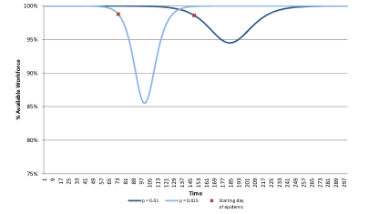
(a) An absolute perspective in time: Curves start from the moment infectives are introduced into the susceptible population.

(b) A planner’s perspective: Curves for both epidemics start from the moment an epidemic is declared.

Figure 1: Availability of workforce as epidemic progresses for different values of $p$.

Given this uncertainty, it is likely that basing the response to an epidemic on a fixed estimate for $p$ is incorrect. To illustrate the impact of such a decision we refer the reader to Figure 1. It shows the availability of staff as a function of time, for different two values of $p$, from two different perspectives. Figure 1a shows how the workforce becomes ill at the actual time it happens. In contrast, 1b presents these curves all starting from the time the epidemic is declared. Indeed, a planner deploying a contingency plan at the moment an epidemic is declared would be interested in the preparing for different scenarios according to what is shown in 1b, rather than 1a. This point will be touched upon again in Section 6.2.

Consider a baseline of $90\%$, i.e. the system is considered to be performing poorly if fewer than $90\%$ of the staff is available. For $p=0.015$ this period spans days $18$ through $37$ (from the declaration of the epidemic), whereas for $p=0.01$ the baseline is not reached. As expected, the epidemic is more severe for higher values of $p$; however, somewhat lower values of $p$ result in longer-lasting epidemics. In particular, $p=0.01$ results in an extended period of time (days $13$ through $69$) where even though staff availability is above the baseline, it is still significantly below $100\%$. If, in the above example, $p$ were unknown, a planner would have to carefully ration scarce resources over a nearly month-long period. If the planner were to assume a fixed value for $p$ throughout the epidemic, then the example suggests allocating comparatively higher levels of surge staff to earlier periods of time, to overcome the higher shortfalls to be expected in the case of higher values for $p$. Of course, this higher level of initial allocation needs to be carefully chosen to obtain maximum reward.

Consider now Figure 2, which shows the impact of a change in $p$ in the midst of an epidemic. Here, $p$ changes from $0.012$ to $0.03$ on day $130,$ $28$ days after the epidemic has been declared. Thus, for more than half of the epidemic, the disease spreads slowly and even though the $90\%$ baseline is approached, it is not reached. However, after the change in $p$ the epidemic becomes severe and a significant shortfall arises. This type of variability would be especially problematic when resources are limited. The epidemic, on the basis of observations of its initial progression, would likely be classified as relatively mild, and, perhaps, action might be taken to at least partially abandon the surge staff buildup. However, if the a change in $p$ as shown in Figure 2 were plausible, then a careful planner would have to hedge by hold backing staff so as to handle the potentially critical situation in later periods. Should the change in $p$ not take place, the chart indicates that any held back staff would essentially be wasted. And should the change take place somewhat earlier, then the opportunity cost is significantly higher. The critical question, of course, is whether this type of virus behavior is possible. As far as we can tell, current knowledge of the influenza virus cannot categorically reject a change in $p$ as shown, although planning for such a change might be construed as an overly conservative action. Thus, it remains to be seen if a robust strategy that can protect against a change in $p$ entails higher cost or other compromises.

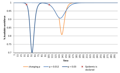
(a) An absolute perspective in time: Curves start from the moment infectives are introduced into the susceptible population.

(b) A planner’s perspective: Curves for all three epidemics start from the moment an epidemic is declared.

Figure 2: Availability of workforce as epidemic progresses for different values of $p$.

In this paper we model the variability of the product $\lambda_{j}p$ using techniques derived from robust optimization. For ease of exposition, we assume that the infectivity probability $p$ is uncertain, and that the values for the contact rates $\lambda_{j}$ are fixed (and known); thus the contact probabilities $\beta_{t}$ are also fixed. Our goal is to produce surge staff deployment strategies that are robust with respect to variability of $p$ in a number of models of uncertainty. Robust optimization provides an agnostic methodology for assessing competing allocation plans and for computing good plans according to various criteria. Above, we described two such criteria. Our optimization procedures are fast and flexible, making it possible to evaluate multiple plans and different levels of conservatism in a practicable time frame.

5 Performance Measures

Personnel shortage during an epidemic may jeopardize the continuity of operations of critical infrastructure organizations. To gauge the impact of this shortfall, we consider cost functions that model two scenarios. In the first one the organization requires at least certain percentage of personnel present to operate. This could be the case of water and energy plants, as mentioned in [29]. The second scenario uses classic queueing theory to measure the simultaneous impact of the decrease in number of available workers and the change in demand for the service that the organization provides. Health care institutions would be clear examples in this context.

5.1 Threshold functions

Here we model an organization that requires a minimum number of staff in order to operate under normal conditions. We further assume that this “minimum” is a soft constraint in the sense that if the available staff should fall below the threshold, the organization will still manage to operate, but at very large cost. This could be the case, for example, if the organization is able to purchase output or hire staff from another source (such as a competitor) or if it is able to reduce its level of service or output, at cost.

To model this behavior, we assume that operating costs at each point in time are given by a convex piecewise linear function. This function is represented as the maximum of $L$ linear functions, with slopes $\sigma_{L}<\sigma_{L-1}<\ldots<\ldots\sigma_{1}=0$ and intercepts $k_{L}>K_{L-1}>\ldots>K_{1}=0$. Thus, denoting by $\omega_{t}$ the work force level at time $t$ and $z_{t}$ the cost associated with time period $t$, we have

$$z_{t}=\max_{1\leq i\leq L}\left\{\sigma_{i}\,\omega_{t}+k_{i}\right\}.$$ (7)

5.2 Queueing models

We are interested in modeling basic queueing systems where both the service rate and the incoming demand rate are affected by the evolution of the epidemic. For each time period $t$, denote the average incoming demand rate by $\zeta_{t}$ and let $s_{t}$ denote the number of available servers (staff). The system utilization at time $t$, using an M/M/$s_{t}$ queueing model, is given by

$$\rho_{t}=\frac{\zeta_{t}}{s_{t}\mu}.$$ (8)

As it is well known, $\rho_{t}$ and related quantities are good indicators of system performance. In our simulations of severe epidemics, $\rho_{t}$ can grow larger than $1$, a situation that depicts a system that is catastrophically saturated (a situation observed during 2010’s H1N1 pandemic[50, 18]) and consequently system performance will drastically suffer. Accordingly, we choose as a reasonable representative of “cost” incurred at time $t$ an exponentially increasing function of $\rho_{t}$. In particular we consider $e^{\rho_{t}-\delta}$ (for small $\delta>0$) which we approximate with a piecewise-linear function, much as in Section 5.1. Other alternatives are possible. For example, one could use a traditional measure of system performance, such as average queue length for an M/M/$s_{t}$ system, computed using a shifted $\rho_{t}$, i.e. a quantity $\hat{\rho}_{t}=\rho_{t}-\delta$ for appropriate $\delta$.

In a regime where $\rho_{t}$ is close to (but smaller than) $1$, one could use one of the popular measures of queueing system performance as “cost” – or use $\rho_{t}$ itself as the cost.

5.3 Other cost functions

Other situations of practical relevance besides the two considered above are likely to arise. Our robust planning methodology, described below, is flexible and rapid enough that many alternate models could be accommodated. Moreover, we would argue that in the context of the cost associated with staff shortfall, any reasonable cost function would be, broadly speaking, increasing as a function of the shortfall. The approach described above approximates cost, in the two cases we listed, using piecewise-linear convex functions, and we postulate that many cost functions of practical relevance can be successfully approximated this way.

6 Robust Models

We now describe our methodology for the robust surge staffing problem. We will first describe our uncertainty model, then the deployment policies we consider, and finally the robust optimization model itself. In what follows, we make the assumption that the total quantity of surge staff is small enough that their deployment does not affect the evolution of the epidemic in the SEIR model, in particular the values $\beta_{t}$.

6.1 Uncertainty models

Let $p_{t}$ denote the probability of contagion at time $t$ (time measured relative to the declaration of the epidemic). The model for uncertainty in $p$ that we consider embodies the notion of increasing uncertainty in later stages of the epidemic. We will fist describe the model and then justify its structure. We assume that there are four given parameters $p^{L},p^{U},\hat{p}^{L},$ and $\hat{p}^{U}$. The model behaves as follows:

There is a time period $\breve{t}$, unknown to the planner, such that for $1\leq t\leq\breve{t}$, $p_{t}$ assumes a constant (but unknown to the planner) value in $[p^{L},p^{U}]$, and for $\breve{t}<t$, $p_{t}$ assumes a constant (and also unknown to the planner) value in $[\hat{p}^{L},\hat{p}^{U}]$.

We stress that $\breve{t}$ is not known to the planner. We are interested in cases where $\hat{p}^{L}\leq p^{L}$ and $p^{U}\leq\hat{p}^{U}$, that is to say, the period following day $\hat{t}$ exhibits more uncertainty than the initial period. We can justify our model as follows. In the event of an epidemic, a planner would be able to obtain some information on the spread of the epidemic in the period leading to the actual declaration of the epidemic, resulting in a (perhaps tight) range of values $[p^{L},p^{U}]$. As we will discuss below (Section 6.2) we are interested in surge staff deployment strategies with limited flexibility, i.e. requiring staff commitment levels that are prearranged.

In this setting, at the point when the epidemic is declared, the planner would deploy a staff deployment strategy. A prudent planner, however, would not simply accept the range $[p^{L},p^{U}]$ as fixed. In particular, if at first the epidemic is mild (small $p^{U}$) the planner might worry that a change, such as sudden drop in temperature, could effectively increase $p$ beyond $p^{U}$. Note that a change in weather would not simply change the contact rates, $\lambda;$ it might produce other environmental changes (such as decreased ventilation); further, it is known that the influenza virus has higher transmissibility in colder and drier conditions [44, 37]. we model such changes, collectively, through changes in $p$. Should the change take place, a staff surge strategy that consumed most available staff in the earlier part of the epidemic would be ineffective.

As a means to avoid this overcommitment of resources to early phases of the epidemic, we can assume that a second and more virulent regime of the epidemic could be manifested at an unknown later time. We can parameterize this later regime by assuming a range $[\hat{p}^{L},\hat{p}^{U}]$ with, for example, $\hat{p}^{L}=p^{L}$ and $\hat{p}^{U}>p^{U}$. The exact relationship between the two values $\hat{p}^{U}$ and $p^{U}$ is a measure of the conservativeness or risk-aversion of the decision-maker. We will touch upon this issue later.

Of course, exactly the reverse could happen: the epidemic could become milder in the second stage. This could take place as a function of changes in public behavior due to non-pharmaceutical interventions (see [8, 22]) resulting in a (difficult to accurately predict) decrease in infectivity. In that case, a surge strategy that defers most staff deployment to the second stage of the epidemic could also be ineffective. The challenge is how to properly hedge in view of these extreme situations, and other intermediate situations that could also arise.

6.2 Deployment strategies

We make several assumptions that constrain the feasible deployment patterns. First, we assume that a surge staff member, when deployed, will be available for up to $\tau$ time periods, provided that he or she does not get infected first - if that happens, this person will be removed from the system and will not available for deployment in the future. We also assume that the pool of available surge staff over the planning horizon is finite. Finally, there is a maximum quantity of surge staff that can be summoned on any given time period. More detailed models are possible and easy to incorporate in our optimization framework.

In this paper we will focus on offline, or fixed strategies. More precisely, we assume that a deployment vector is computed immediately after an epidemic is declared, on the basis of the available information. From a formal perspective, the deployment vector is obtained as follows:

• First, the epidemic must be declared. As indicated in Section 2.1, this takes place as soon as the percentage of infected individuals exceeds some (small) threshold.

• Based on data available at that point, estimates are constructed for the various SEIR parameters. In particular, the ranges $[p^{L},p^{U}]$ and $[\hat{p}^{L},\hat{p}^{U}]$ for $p$ (see Section 6.1) are constructed.

• Using as inputs the population statistics, the cost function, the nominal SEIR model parameters, and the uncertainty model for $p$, we compute the deployment vector $h=[h_{1},h_{2},\ldots,h_{T}]$, where $h_{t}$ indicates the number of staff procured $t$ time periods after the declaration of the epidemic. The parameter $T$ is chosen large enough to encompass one epidemic wave and will be discussed later.

We next address some points implicit in (1)-(3). First, recall that in the SEIR framework the formal epidemic will have a starting point which precedes the time period when an epidemic is actually declared. The exact magnitude of this run-up period is not known to a decision maker. In all our notation below (as in (2) above), “time period 1” refers to the time period where the epidemic was declared, that is to say, we always label time periods by the amount elapsed since the declaration of the epidemic. When using the SEIR machinery to simulate an epidemic, of course, we always proceed as in the formal model, and we merely relabel as “time = 1” that period where the declaration condition is first reached (since that would be the start of the epidemic as far as a planner is concerned).

Also, we assume that the epidemic is correctly declared, that is to say, the first day in which the criterion in Section 2.1 applies is correctly observed. In practice, this observation would include noise (for example, due to individuals infected by a different strain) but we make the assumption that the resulting decrease in strategy robustness is small.

Item (2), the estimation of the SEIR model and in particular the construction of the initial range $[p^{L},p^{U}]$, gives rise to a host of other issues that are outside the scope of this paper (but are nonetheless important). We assume that at the time the epidemic is declared there is enough data (however incomplete, and noisy) to enable the application of $robust$ least squares methods (see e.g. [15]) to fit an SEIR model, and that the model is sufficiently accurate to permit point estimates for all parameters other than $p$. Having constructed the initial range $[p^{L},p^{U}]$, the later range $[\hat{p}^{L},\hat{p}^{U}]$ is constructed on the basis of (a) risk aversion, and (b) environmental considerations. The role of (a) is clear -for example, we could obtain $\hat{p}^{U}$ by adding to $p^{U}$ a multiple (or fraction) of the standard deviation of $p$ in the observed data. As an example for (b), an epidemic that starts in late-Autumn might possibly become more infectious as colder weather develops.

Another point concerns the time horizon, $T$, for the SEIR model (see Section 3) which to remind the reader is measured from the point that the epidemic is declared. It is assumed that $T$ is large enough to handle an epidemic of interest. If we assume a fixed (but unknown) $p$, then the milder (i.e., less infective) epidemics will tend to run longer, but, significantly, will also be less disruptive. Higher values of $p$ give rise to sharper epidemics in the near term. From a technical standpoint, the parameters $p_{L}$ and $\hat{p}_{L}$ can be used to construct estimates for $T$. In order to be sure that we capture as much of an epidemic as possible, in this study we will use values for $T$ up to 150, which according to our experiments seems more than adequate.

One could consider models of epidemics spanning, for example, a one-year period, with multiple epidemic “waves”. If some of these waves are very prolonged then they will necessarily be mild waves for long periods of time. As a result, during such long, mild epidemic periods (1) the social cost will be low, and (2) a significant pool of the population will become sick and as a result become immune to the virus. Consequently, future epidemic waves will necessarily be milder and cause decreased social cost (so surge staff will be less critical). On the other hand, over a long period we could have well-separated strong epidemic waves. However, we would argue that from the perspective of surge staff deployment, each such wave should be handled as a separate event, with its own surge staff deployment strategy.

A significant element in our approach is that it produces a fixed deployment vector $h_{1},\ldots,h_{T}$ which, from a formal standpoint, will be applied regardless of observed conditions. Of course, the strategy should be interpreted as a template and a planner would apply small deviations from the planned surge levels, as needed. In any case, we have focused on this assumption for practical reasons. Having a pre-arranged schedule greatly simplifies the logistics of deploying possibly large numbers of staff, especially if many of the staff originate from geographically distant sources.

A broader class of models would allow for on-the-fly revision of a strategy in the midst of an epidemic, which would allow a planner to dynamically react to changes in the epidemic.

However, a significant underlying issue concerns the actual flexibility that would be possible under a virulent epidemic. We expect that large, sudden changes in deployment plans may be difficult to implement. In particular, if a significant and unplanned increase in surge staff is needed, it may prove impossible to rapidly attain this increase; and by the time the surge staff is available a severe peak of the epidemic may already have taken place. See Section 7.1.5 for some experimental validation of these views.

A different type of dynamic strategy would implement many, but small corrections as conditions change. We will discuss examples of such strategies (and appropriate modifications to our methodology) in Section 8; an issue in this context is the callibration of our statement “as conditions change” in an environment that will be characterized by noisy, partial and late data.

6.3 Robust problem

We can now formally state the problem of computing an optimal robust pre-planned staff deployment strategy. Let $h$ denote a deployment vector and ${\cal H}$, the set of allowable deployment vectors. Let $\vec{p}=(p_{1},p_{2},\ldots,p_{T})$ be a vector indicating a value of $p$ for each time period. Define

$$V(h\,|\,\vec{p}) := h p_{t} t$$ cost incurred by deployment vector , if the infection probability equals at time . (9)

[Here we remind the reader that time is measured relative to the declaration of the epidemic.] Let ${\cal P}$ indicate a set of vectors $\vec{p}$ of interest; our uncertainty set. Our robust problem can now be formally stated, as follows:

Robust Optimization Problem $\displaystyle V^{*}$ $\displaystyle:=$ $\displaystyle\min_{h\in{\cal H}}\max_{\vec{p}\in{\cal P}}~{}V(h\,|\,\vec{p}).$ (10)

Problem (10) explicitly embodies the adversarial nature of our model. Given a choice of vector $h$, a fictitious adversary chooses that realization of the problem data (the contagion probabilities) that maximizes the ensuing cost; the task for a planner is to minimize this worst-case cost. The set ${\cal H}$ describes how staff deployment plans are constrained. In our implementations and testing, we assume that any deployed staff person works for a given number $\tau$ of time periods, or until he or she gets sick; following this period of service this person will not be available for re-deployment. We also assume that whenever surge-staff is called up, there is a one-period lag before actual deployment (this assumption is easily modified to handle other time lags).

Finally, we model the impact of the epidemic on surge staff using the SEIR model with parameters as for the workforce group ($\lambda^{2}_{t}$ and $\mu_{E_{2}}$), and we assume that the total quantity of available surge staff is small enough so as to not modify the outcome of the epidemic.

In Appendix A we will present an efficient procedure, based on linear programming, for solving problem (10) to very tight numerical tolerance.

7 Numerical Experiments

In this section we investigate the structure of the optimal robust policies by numerical experiments. First, it is worth raising a point concerning “approximate” vs “exact” solutions. Our algorithms construct numerically optimal solutions to the formal problems they solve; nevertheless, as argued above, our models approximate real problems. Again, we postulate that given the context (i.e. the behavior of social entities) an approximation is the best we can hope for; moreover we expect that robust strategies computed for the approximate models will translate into actual robustness in practice. This last feature can at least be experimentally tested through simulation, as we present via examples in this section.

In order to assign numerical values to the various parameters in our models, we followed the existing literature and consulted with various experts [44, 40]). The numbers in the literature may vary significantly depending on various factors such as the location where the study took place, the underlying model for which the parameters were calibrated, and the epidemic wave of study. For example, published values for the influenza $R_{0}$, the number of secondary transmissions caused by an infected individual in a susceptible population, range from $1.68$ to $20$ [38]. Our main sources are listed in Table 1.

Table 1: List of references for different parameter values.

Parameter	Description	Value(s)	Reference
Epidemic related parameters
$p$	Probability of contagion	$[0.02,0.16]$a	[52]
		$\{0.07,0.09,0.12\}^{b}$	[33]
$\lambda$	Contact rate	$47.48$ (per day)	[51]
		$35$ (per day)c	[33]
$\mu_{E}^{-1}$	Latent period	$1$ day	[26]
		$1.9$ daysd	[35]
		$1.25$ days	[19]
		$1.48\pm 0.48$ days	[19] and within
$\mu_{R}^{-1}$	Infectious period	$2$ days	[26]
		$4.1$ days	[35, 34]
		$4.1$ dayse	[34]
$1-f$	Mortality rate	$0.02$	[35]
		$0.002$ per dayf	[19]
		$1.2$%g	[9]
		$0.05$g	[34]
$R_{0}$	$R_{0}$	$1.68$ to $20$h	[38] and within
		$1.73$i	[51]
		$2.5$j	[34]
	Length of pandemic wave	$8-12$ weeks	[19]
Hospital related measures
$\zeta$	Patient arrival rate	2,800 ILI cases/dayk	[34]
$\mu$	Service rate	$24-30$min/patientl	[23]
$\rho$	Occupancy rate	Average of $85\%$m	[12]
$\delta$	Increase in demand for health care	up to $50$%	[1]
Miscellaneous
	Seasonal threshold	$[0.06,0.076]$ weeklyn	[16]
	Epidemic threshold	$[0.064,0.08]$ weeklyn	[16]
	ILI National Baseline	$2.4\%$ weeklyo	[16]
$\theta$	Transmission reduction factor	$29$% to $37$%p	[9]
a 1957 wave in the Netherlands
b Values of $p$ for different socially active groups
c Weighted average of different age groups presented in the paper
d 1957 pandemic wave
e Untreated symptomatic
f Treated symptomatic
g Overall ILI case-fatality ratio during 2009 H1N1 pandemic in Mexico
g Spanish Flu fatality rate
h From multiple studies
i 1957 wave
j Min 1.5, Max 6
k Data for Singapore, 2005. Population then was about 4.35 million people
l Emergency Department, New York Presbyterian Hospital
m Maintained beds capacity for New Jersey Hospitals, 2005
n The threshold is for percentage of deaths caused by pneumonia and influenza.
It is different for each week throughout the year.
o Percentage of influenza-like illness (ILI) patient visits reported through the U.S. Outpatient ILI Surveillance Network.
p Estimated effect of social distancing measures during H1N1 epidemic in Mexico, 2009

7.1 Health care setting

We now present examples modeling a hospital of the size of New York-Presbyterian Hospital in New York City under slightly different scenarios. Staff at this hospital amounted to $19,376$ in 2010 (we have rounded this up to $20,000$) and served a population of approximately 900,000 people [30]. We used these numbers as a baseline to obtain different scenarios with different initial conditions.

In the event of an epidemic, hospitals will be likely to experiment surge demand trailing the incidence curve. We use the queueing-based cost function to capture both shifts in demand and workforce availability while the epidemic ensues. This increase in demand for service is modeled by adding a proportional factor of $I^{1}_{t}$ to the average arrival rate of patients when we compute the system’s occupation rate, $\rho_{t}$:

$$\rho_{t}=\frac{\bar{\zeta}+\delta\,I^{1}_{t}}{s_{t}\mu}.$$ (11)

7.1.1 Example 1

For this example we assume 3,000 surge staff members are available, each of which will be called up for at most one period of service lasting one week. If the member becomes infectious while on call, then service is terminated with no further future availability.

We used the uncertainty model in Section 6.1 which allows $p_{t}$ to change once. The change is further constrained to take place within a fixed range of time periods.

The social contact model assumed the nonhomogeneous-mixing rule described in section 3.1.2. Additionally, we assumed that social contact rates were dampened by a factor of $30$% while the epidemic is declared; that is, during the days in which the growth of infectives is higher than a given threshold. Additionally, we assumed an epidemic is declared only once. In other words, once the rate of infectives slow down below the epidemic threshold, the epidemic is considered to be terminated.

The parameter values for this example are summarized in Table 2; the range of days where $p$ is allowed to change are measured from the start of the epidemic (rather than the day the epidemic is declared).

Table 2: Parameter values for example 1

Parameter	Description	Value(s)
Epidemic related parameters
$P$	Uncertainty set	$[0.01,0.012]\times[0.0125,0.0135]$
	Possible days of change	$\{140,\dots,160\}$
$(\Lambda_{1},\Lambda_{2})$	Contact rates	$(30,35)$ per day
$\mu_{E}^{-1}$	Latent period	$1.9$ days
$\mu_{R}^{-1}$	Infectious period	$4.1$ days
$1-f$	Mortality rate	$0$
$R_{0}$	$R_{0}$	$[1.24,1.48]$
	Deployment threshold	$2.4\%$ weekly
Population parameters
$N_{1}$	General population size	900,000
$N_{2}$	High risk population size	20,000
$[I_{1},I_{2}]$	Initial infectives	[5,0]
System Utilization (Queueing setting)
$\bar{\zeta}$	Patient arrival rate	500 per day
$\mu$	Service rate per person	$30$ patients per day
$\rho_{0}$	Initial occupation rate	0.875
$\delta$	Daily increase in demand for health care	$0.07$%
Deployment parameters
	Total number of available volunteers	$3,000$
$\tau$	Length of stay (w/o sickness)	7
	Deployment lag	1

In what follows, the staff deployment plan computed by our algorithm will be called the Robust Policy. To gauge its usefulness, we study its performance under different scenarios, each of which is defined by a tuple $(p_{1},p_{2},d)$ representing the initial probability of contagion ($p_{1}$), the time period where it changes ($d$) and the value to which it changes ($p_{2}$).

A natural alternative to the Robust Policy is that which best responds to what could be construed as a worst-case scenario - the scenario which yields the highest cost when no contingency plan is implemented. Such a strategy can be obtained by solving a linear program as described in (18) once the tuple that implies the evolution of $p_{t}$ in this scenario is identified. In this example such tuple is given by $(0.01092,0.0135,140);$ we will term it the No-Action-Max-Cost tuple, and the deployment strategy which achieves minimum cost under this tuple the Naïve-worst-case Policy. We compare the Naïve-worst-case and Robust Policies under the following scenarios:

1. No-Action-Max-Cost tuple $(0.01092,0.0135,140)$;

2. The tuple that achieves highest cost if the Naïve-worst-case Policy is implemented; and

3. The tuple that achieves highest cost if the Robust Policy is implemented.

Table 3: Results. Example 1.

Scenario / Strategy / tuple		No Intervention	Robust Policy	Naïve-worst-case Policy
1	Cost	4.5812	0.0495	0.0000
No intervention	Maximum $\rho$	1.0481	1.0018	0.9999
(0.01092,0.0135,140)	# days $\rho\geq$ 1	28	8	0
2	Cost	1.4300	0.0500	0.7100
Naïve-worst-case Policy	Maximum $\rho$	1.0210	1.0020	1.0185
(0.01172, 0.0135, 140)	# days $\rho\geq$ 1	20	8	13
3	Cost	1.6938	0.0521	0.6862
Robust Policy	Maximum $\rho$	1.0236	1.0027	1.0170
(0.01168, 0.0135, 140)	# days $\rho\geq$ 1	21	7	12

Results are summarized in Table 3. In Scenario 1 the Robust Policy presents a cost improvement of almost $99\%$ over the no-intervention policy. While it is not completely able to prevent $\rho$ from exceeding $1$, it reduces the number of critical days from 28 to 8, and the maximum $\rho$ from $1.05$ to below $1.002$. Indeed, the undesirable instability in which a system is put through when $\rho>1$ is heavily penalized with the use of the exponential function in our objective function (see 5.2). On the other hand, under Scenario 1 the Naïve-worst-case Policy reduces the cost to $0$; that is, there is no day in which $\rho$ is greater than $1$. Without doubt, it represents a better solution than the Robust Policy for this particular case. This result is expected; the solution derived from that single linear program is specialized in this scenario, while the Robust Policy, having to hedge against other possible bad cases, does not perform as well in this instance.

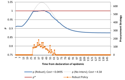
(a) Scenario 1:Effectiveness of Robust Policy

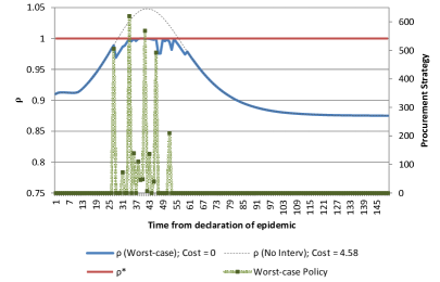
(b) Scenario 1:Effectiveness of the Naïve-worst-case Policy

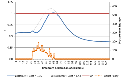
(c) Scenario 2:Effectiveness of Robust Policy

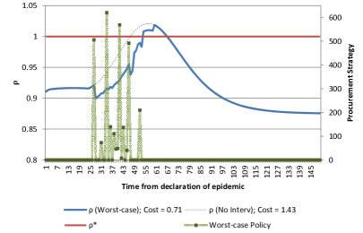
(d) Scenario 2:Effectiveness of Naïve-worst-case Policy

Figure 3: Reduction in $\rho$ obtained by the Robust and Naïve-worst-case deployment strategies under two scenarios: 1) Worst-case scenario given that no policy is implemented, and 2) Worst-case scenario given that Naïve-worst-case Policy is implemented.

The situation is considerably different, however, when we look at Scenario 2, which achieves the highest cost when the Naïve-worst-case Policy is being implemented. In this case, the Robust Policy performs much better than the Naïve-worst-case Policy: the former reduces the cost of this scenario by $96.5\%$, while the latter does so by only $50\%$; the Robust Policy reduces the number of critical days from $20$ to $8$ days, while this number jumps to $13$ for the Naïve-worst-case Policy. The maximum value of $\rho$ is $1.002$ for Robust Policy and $1.018$ for Worst-Scenario, compared to $1.021$ with no intervention.

This fact is further illustrated in Figure 3, where we compare the behavior of $\rho_{t}$ with and without interventions for Scenarios 1 and 2 together with the deployment patterns. We note that the Naïve-worst-case Policy deploys staff around in large, sharp bursts between days $27$ and $52$. The Robust Policy deployment, on the other hand, trails $\rho$ in Scenario 1 in a smoother way by calling in personnel in smaller batches, and also over a longer period of time: $36$ days. This shows the importance of Scenario 1 as the costliest case and, at the same time, how the strategy hedges against scenarios where the epidemic has its peak later (than under the No-Action-Max-Cost tuple), even if not so aggressively. In particular, the last wave of staff deployed by the Robust Policy (on days $54,58,$ and $63$) could seem somehow wasteful under Scenario 1; however their utility is displayed under Scenario 2, where the Robust Policy tackles a delayed, weaker $\rho$ peak much more effectively than the Naïve-worst-case Policy. Because an unstable system builds up a queue exponentially fast, even this small changes in $\rho$ could translate in significant difference in the load experienced by the system.

A similar situation is presented in Scenario 3, as illustrated in Table 3. The Naïve-worst-case Policy is not as effective as handling what would have been a milder epidemic, while the Robust Policy performs consistently well. In fact, this is the worst scenario for the Robust Policy; nevertheless it manages to significantly outperform the Naïve-worst-case Policy here as well. Indeed, a feature of the Robust Policy is its near-uniform behavior under all scenarios; this epitomizes the use of the term ’robust’.

7.1.2 Example 2

To further illustrate the structure of the Robust Policy under different scenarios, we now consider the previous example with some modifications. Here, the uncertainty set is $p$ lies in the interval $[0.01,0.0125]$ throughout, but can change values once on any day in the range $\{100,\dots,115\}.$ $R_{0}$ is now between 1.24 and 1.54. The total number of available volunteers is $2,000$ and the contact rates are not dampened while the epidemic is being declared. All other data remains as in the first example.

Following the same logic as in the previous example, we present the Robust Policy and compare it to the Naïve-worst-case Policy (obtained as before by solving the linear program associated with the worst-case tuple of our uncertainty set). We present results for the same three scenarios: the No-Action-Max-Cost tuple, the costliest tuple for the Naïve-worst-case Policy, and the costliest tuple for the Robust Policy, respectively. This fact hints on the nonconvexity of the problem, a topic we will touch upon later in this section.

Table 4: Results. Example 2.

Scenario / Intervention / Tuple		No Intervention	Robust Policy	Naïve-worst-case Policy
1	Cost	3.8332	0.0280	0.0066
No intervention	Maximum $\rho$	1.0410	1.0012	1.0003
(0.0125, 0.0125, 100)	# days $\rho\geq$ 1	27	10	6
2	Cost	3.5906	0.0280	0.0542
Naïve-worst-case Policy	Maximum $\rho$	1.0393	1.0019	1.0025
(0.01235, 0.0125, 112)	# days $\rho\geq$ 1	26	7	8
3	Cost	3.7320	0.0295	0.0379
Robust Policy	Maximum $\rho$	1.0403	1.0010	1.0017
(0.01015, 0.0125, 101)	# days $\rho\geq$ 1	26	10	10

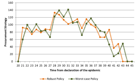
Figure 4: Example 2. Deployment Strategies

Table 4 displays the results. The Robust Policy is worse than the Naïve-worst-case Policy in the first instance, while keeping a fairly consistent and low cost for the other scenarios; where the Naïve-worst-case Policy does not perform as well. What is worth noting is that, unlike in the previous example, the structure of the deployment strategies is much more similar (see Figure 4); nevertheless, the small differences make the Robust Policy more resilient to other scenarios. A second observation regards the structure of the worst-case tuples evinced by the policies. In this example the No-Action-Max-Cost tuple corresponds to having an epidemic with a fixed probability of contagion $p=0.0125,$ the highest in the interval of the uncertainty set. However, the costliest tuples for the Robust and Naïve-worst-case policies are quite different.

7.1.3 Cost-benefit analysis

We now present a cost-benefit analysis on the number of surge staff available. We took this example as a base case and recomputed the optimal Robust and the Naïve-worst-case policies assuming $1,000$, $1,500$, $2,500$, and $3,000$ available surge staff. Table 5 displays the change in the worst-case cost given that the corresponding policy is being implemented and its corresponding cost if no contingency plan had been put in place. Similarly, the change in the maximum value of $\rho$ and the number of days that $\rho$ is at or above $1$ are also presented. The last row of the table shows the ratio between the change in the worst-case cost and the change in the number of available surge staff. For example, when there are $1,500$ volunteers available, there is a change in the cost of $0.156\%$ for each of the $500$ that are now not at hand. At the same time, the benefit obtained per additional worker available decreases for both the Robust and the Naïve-worst-Case Policy, but more so for the latter. This is again because the Robust Policy allocates the additional staff to cover up for different bad cases, while the Naïve-worst-case Policy has only one scenario to focus on. This is depicted in Figure 5: for the cases in which the Robust Policy has more surge staff available, more people are hired towards the end of the planning horizon, while the Naïve-worst-case Policies look to tackle the system congestion early after the epidemic has been declared.

Table 5: Cost-Benefit Analysis for different quantities of available surge staff.

	Robust Policy					Naïve-worst-case Policy
Total staff deployed	1,000	1,500	2,000	2,500	3,000	1,000	1,500	2,000	2,500	2,579
Worst-case cost	1.756	0.8183	0.0295	0	0	1.7535	0.8114	0.0542	0.0190	0.0156
Worst-case cost (No Int)	3.8332	3.8332	3.732	3.8332	3.8332	3.8332	3.8332	3.6077	3.6997	3.5906
Maximum $\rho$	1.02	1.02	1.001	0.999	0.998	1.02	1.01	1.002	1.002	1.002
Maximum $\rho$ (No Int)	1.04	1.04	1.04	1.04	1.04	1.04	1.04	1.04	1.04	1.04
# days $\rho\geq$ 1	27	27	10	0	0	27	27	8	3	2
# days $\rho\geq$ 1 (No Int)	27	27	26	27	27	27	27	26	26	26
$\frac{\Delta\mbox{Cost}}{\Delta\mbox{Surge Staff}}$	0.345%	0.158%	-	-0.006%	-0.003%	0.345%	0.156%	-	-0.002%	-0.002%

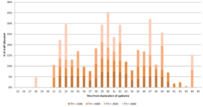
(a) Robust Policies.

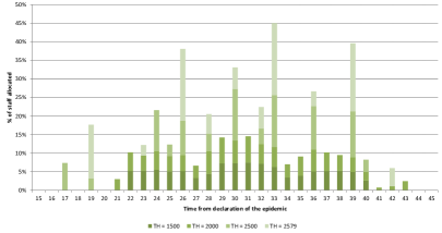
(b) Naïve-worst-case Policies.

Figure 5: Distribution of the deployment strategies for different quantities of available surge staff.

7.1.4 Nonconvexity

As the examples above make clear, the systems we study can be strongly dependent on the choice of $p$, with clear nonlinearities and nonconvexities. This justifies the use of robustness in the design of response strategies.

To further study the dependence on $p$, we considered the cost of a set of strategies when $p$ is constant throughout the epidemic. Figure 6a plots the objective function as a function of $p$ in the interval $[0.0115,0.0125]$ when there is no intervention; clearly cost is monotone increasing in $p$. However, Figure 6b shows similar plots for three strategies computed by our algorithms. These curves are certainly not monotonic and, not surprisingly, particular values of $p$ are able to exploit relative “gaps” in deployment.

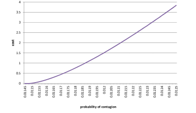
(a) Total cost as a function of $p$ under no intervention.

(b) Total cost as a function of $p$ under 3 different strategies.

Figure 6: Total cost of an epidemic as a function of $p$ under a)No intervention, and b) Three different deployment policies.

7.1.5 Out-of-sample tests

The set of experiments we present below amount to out-of-sample testing. We build on Example 1 (Section 7.1.1), in which the initial uncertainty interval for $p$ was $[0.01,0.012]$, and the second interval was $[0.0125,0.0135]$; $p$ was allowed to change between days $140$ and $160$. In the tests reported in Tables 6 and 7, $p$ is allowed to change to a value $larger$ than $0.0135$ $and$ allowed to change later than in day $160$. Thus, the experiments go out-of-sample in two ways.

Table 6: Effects of a late change in $p$ on Scenario 3

Worst-case scenario given that the Robust Policy is implemented
Scenarios	Original	Hypothetical 1				Hypothetical 2
$p_{1}$	0.01168	0.01168				0.01168
$p_{2}$	0.0135	0.014				0.015
day epidemic declared	113	113				113
day deployment starts	140	140				140
day change $p$	140	150	155	160	165 -	150	155	160	165
cost Robust Policy	0.0508	0.3268	0.0729	0	0	2.1737	1.4068	0.6282	0.0294
cost No Intervention	4.58	1.6087	0.7619	0.087	0	4.1327	2.6688	1.2427	0.1462

The tests were constructed as follows. First, the epidemic is declared on day $113$ with deployment under the Robust Policy beginning on day $140$, i.e. $28$ days after the declaration. As we saw in Example 1, the costliest tuple should the Robust Policy be implemented is $(0.01168,0.0135,140)$ (thus, $p$ changes on the day of deployment). Table 6 evaluates the Robust Policy (and the No-Intervention policy) against this tuple, and also against tuples of the form $(0.01168,\tilde{p},\tilde{d})$, with $\tilde{p}=0.014,\,\mbox{or}\,0.015$ and $\tilde{d}=150,155,160,$ and $165$ and greater. Table 7 displays the same evaluations, but against the No-Action-Max-Cost tuple $(0.01092,0.0135,140)$, and against tuples of the form $(0.01092,\tilde{p},\tilde{d})$, with $\tilde{p}=0.014,\,\mbox{or}\,\,0.015$ and $\tilde{d}=170,175,180$ and greater.

Table 7: Effects of a late change in $p$ on Scenario 1

Worst-case scenario given that no policy is implemented
Scenarios	Original	Hypothetical 1			Hypothetical 2
$p_{1}$	0.01092	0.01092			0.01092
$p_{2}$	0.0135	0.014			0.015
day epidemic declared	133	133			133
day deployment starts	140	140			140
day change $p$	140	170	175	180	170	175	180
cost Robust Policy	0.0487	0	0	0	0.9827	0.2766	0
cost No Intervention	4.58	0.7684	0.0093	0	2.7795	1.1467	0.0399

In the case of Table 6 we see that for $\tilde{d}=150$ and $\tilde{d}=155$ the cost of the Robust Policy does increase over its worst-case cost under the original robust model ($0.0508$) – however the increase is modest relative to the cost of not intervening. Most importantly, the cost of the Robust Policy decreases rapidly as $\tilde{d}$ moves out of scope of the original model. In fact, the same is true even under the No-Intervention Policy.

This is the salient fact that we want to point out. Its explanation is simple: even though $p$ is increasing to a larger value than originally envisioned, if $\tilde{d}$ is large, the impact of the increase is negligible – the increase is taking place so late, that by then the epidemic (under the initial $p$ value) has largely run its course. In other words, we have a long-running epidemic which, under the Robust Policy, ends up having no impact.

Along the same lines, it is also worthwhile to note that in all cases where the out-of-sample increase in $p$ actually does have a cost impact, the change takes place shortly after the epidemic declaration and very shortly after deployment of the robust strategy begins. These facts indicate that there is a critical period (in this example of duration less than forty days or even shorter) starting from the declaration of the epidemic during which correct action is important. To some degree this supports our model of rolling-out a fixed strategy that deals with the immediate future; should the epidemic “slow down” only to restart much later, a completely new plan would then be deployed.

8 Extensions - policies with recourse

Here we outline two extensions to our approach where the decision-maker can apply recourse when conditions significantly deviate from predictions. From a broad optimization perspective such strategies clearly make sense – why stick with a rigid strategy?. However, we stress that in view of the experiments at the end of the last section, the likely benefit from a dynamic policy would be primarily realized during a period immediately following the epidemic declaration and of relatively short duration. As as a result, a decision maker would likely face severe logistical constraints if attempting to rapidly redeploy large numbers of staff. Thus, a dynamic policy might only be able to perform small changes on a day-to-day basis. From an operational perspective such small changes would of course make sense and would be applied; however the recourse might only amount to a set of small adjustments to a pre-computed strategy.

In both cases that we consider we assume that a decision-maker can only approximately observe the behavior of $p_{t}$ (the value of $p$ at time $t$). The Benders-decomposition solution methodology that we describe in the Appendix can be adapted to handle both models.

8.0.1 Robust optimization with recourse

Assume that uncertainty of $p_{t}$ is modeled using $m$ intervals, or $tranches$, denoted $I_{1},I_{2},\ldots I_{m}$, for some integer $m>0$. In addition, two time periods are given, $J^{min}$ and $J^{max}$. A realization of the uncertain values $p_{t}$ plays out as follows:

• A period $J^{min}\leq J\leq J^{max}$ is chosen, as well as a value $p^{(1)}\in I_{1}$, a tranche $H$, and a value $p^{(2)}\in H$.

• For each $t<J$ we have $p_{t}=p^{(1)}$ whereas for each $t\geq J$, $p_{t}=p^{(2)}$.

In other words, $p_{t}$ is allowed to change values, once. The decision-maker operates as follows. First, a fixed time period, $S$, in which the deployment strategy will be revised is chosen in advance. Then

• At time $t=1$, the decision-maker knows that $p_{1}\in I_{1}$, but does not know its precise value. The decision-maker then produces an initial, or “first-stage” deployment plan indicating the amount of staff to call-up at time $t$, for each $t<S$. Further, $m$ alternative “second-stage” deployment plans (labeled $1,2,\ldots,m$) are announced, each of which specifies the level of staff to deploy at each period $t\geq S$. Each second-stage plan is compatible with the first-stage plan in terms of deployment constraints (such as total staff availability).

• At time $t=S$ the decision-maker observes the tranche that $p_{S}$ belongs to, but not the actual value of $p_{S}$. If tranche $h$ is observed, then second-stage plan $h$ is rolled out on periods $t\geq S$.

Example. Consider a case with three tranches: $I_{2}=[.1,.15],\ I_{1}=[.15,.18],\ \mbox{and}\ I_{3}=[.18,.19]$. Further, $J^{min}=18$ and $J^{max}=60$. A realization of the data is the following: $J=20$, $p^{(1)}=.155$, $H=I_{3}$ and $p^{(2)}=.19$. Thus, for $t<20$ we have $p_{t}=.155$ while for $t\geq 20$, $p_{t}=.19$. Suppose $S=30$. The decision-maker knows that $.15\leq p_{1}\leq.18$; at time $S=30$ the decision-maker observes the tranche $I_{3}$ and thus knows that for $t\geq 30$, $.18\leq p_{t}\leq.19$, leading to an appropriate set of deployments for future periods.

The model we just described is inherently adversarial: it assumes that, subject to the stated rules, data will take on worst-case attributes. This feature can, of course, lead to overly conservative plans. However, the proper statement to make is that the plans will be conservative only if the data (the tranches, in particular) allow it to be so. A different drawback in this model is that an adversary could simply “wait” to change $p$ until just after the review period $S$. As the experiments in Section 7.1.5 indicate, if $S$ is not too small the impact of such a late change in $p$ is much decreased. If $S$ is chosen too large, then the adversary can change $p$ much earlier, and then the impact will be felt before the review can take place. Thus, care must be chosen in selecting $S$. A review strategy that proceeds dynamically is given next.

8.0.2 Stochastic optimization

In contrast to the above, we also outline a model where the contagion probabilities $p_{t}$ behave stochastically. Assume:

• $p_{1}$ takes a random value drawn from a uniform distribution over a $known$ interval $Z$.

• For any $t$, $p_{t+1}=p_{t}\ +\ \epsilon_{t}$, where $\epsilon_{t}$ is normally distributed, with zero mean and small standard deviation (small compared to the width of $Z$).

Thus, $p_{t}$ executes a random walk, starting from $Z$. Let $\bar{p}$ indicate the center (mean value) of $Z$. The decision-maker’s actions, in this model, are as follows.

• At time $t=1$, the decision-maker produces a policy consisting of a triple $(\tilde{h},\,\alpha,\,R)$ where $\alpha\geq 0$, and $\tilde{h}$ is an initial staff surge deployment plan indicating for each $t$ the quantity $\tilde{h}_{t}$, the amount of staff to call-up at time $t$. Finally, the decision-maker also places an additional quantity $R\geq 0$ of surge-staff on $reserve$ (i.e., not yet part of the deployment plan). For notational purposes, write $h_{t}=\tilde{h}_{t}$, for each $t$.

• The decision-maker can revise the plan at any of several checkpoints $t_{1}<t_{2}<\ldots<t_{r}$.

• Consider checkpoint $t_{i}$ ($1\leq i\leq m$). Let

  $$\Theta(t_{i},\bar{p}) = t_{i} p_{t}=\bar{p}$$ the total number individuals infected by time , in the SEIR model where ,

  for $$1\leq t_{i}$$

  $$\Gamma(t_{i}) = actual t$$ the total number of individuals who are infected by time .

  Thus, $\Theta(t_{i},\bar{p})$ is an estimate of the random variable $\Gamma(t_{i})$. We assume that the decision-maker observes, as an estimate for $\Gamma(t_{i})$, a quantity

  $$\nu(i) = \Gamma(t_{i})\ +\ \delta(t_{i}),$$ (12)

  where $\delta(t_{i})$ is normally distributed with zero mean and known variance. Then, the deployment plan is revised as follows. Write

  $$\Delta=\,\frac{\nu(i)\ -\ \Theta(t_{i},\bar{p})}{t_{i}}.$$

  Then, the decision-maker resets

  $$h_{t} \leftarrow h_{t}\ +\ \alpha\,\Delta,\ \ \ \mbox{for each $t_{i}\leq t<t_{i+1}$, and}$$ (13)

  $$R \leftarrow R\ -\ (t_{i+1}-t_{i})\,\alpha\,\Delta.$$ (14)

Comment. The proposed scheme constitutes an example of affine control. The decision-maker computes an initial estimate of the deployment plan (the initial $h_{t}$) which are corrected on the basis of real-time observations, using the parameter $\alpha$ to modulate the corrections. The quantity $\Delta$ indicates the (per-period) deviation between the observed behavior of the epidemic (including “noise”, given by $\delta$) and the predicted behavior as given by $\Theta(t_{h},\bar{p})$.

When $\Delta>0$, the behavior of the epidemic is worse than initially estimated and Rule (13) will increase the near-future surge staff deployment. This increase is drawn from the surge staff held in reserve, as per equation (14). When $\Delta<0$, (14) moves staff back into the reserve ranks.

Note that in order for Rule (14) to be feasibly applied, the resulting $R$ must be $nonnegative$. For this to be the case when $\Delta>0$ we should have $\alpha$ small enough, and, especially, that the initial estimate for $R$ be “high enough.” These are constraints to be maintained in our solution algorithms.

In order to consider algorithmic implications of this model, consider a fixed sample path specifying a value for each $p_{t}$ and for each $\delta(t_{i})$ (see equation (12)). Denote by $T$ the length of the planning horizon. Recall that in the stochastic model the decision-maker announces, at $t=1$, a triple $(\tilde{h},\alpha,R)$. We have:

Lemma 8.1

Under the given sample path the cost incurred by the policy $(\tilde{h},\alpha,R)$ (as per rules (b)-(c) ) is given by a linear program whose right-hand side is an affine function of the $\tilde{h}_{t}$ and $\alpha$.

As a consequence, we expect that several well-known methodologies for stochastic optimization, such as sample average approximation [46], [47] and stochastic gradient schemes [45], [32], will be well-suited for our problem.

9 Discussion

The potential impact of a severe influenza epidemic on essential services is a matter of critical importance from a Public Health perspective. There are current concerns that an influenza virus might mutate into a highly contagious strain for which humans have little or no immunity, resulting in a rapid widespread of the disease. In the event of such an epidemic, or pandemic, organizations that provide critical social infrastructure, such as health care clinics, police departments, public utilities, food markets and supply chains are likely to face severe workforce shortage that would jeopardize their continuity of operations. In particular, at the most critical stage of the epidemic, health care clinics would be required to provide care for an extraordinary number of patients, and thus could ill-afford staff shortfalls. To address these issues, the CDC and the HHS Department have urged organizations to design contingency plans. As part these plans, organizations would deploy emergency ’surge’ staff to compensate for a potential deficit in workers’ availability.

The intelligent design of such contingency plans would necessarily model the spread of the epidemic. In the case of a new strain of the influenza virus, such modeling entails incorporating significant uncertainty: as far as we know, there are no clear ways of accurately predicting the transmissibility of a new virus strain. Moreover, it has been suggested that the effective contagion rate may change under different environmental conditions, such as weather, which are likewise unpredictable. Additionally, social patterns may change during the epidemic, for example due to the implementation of public health measures such as quarantine or social distancing.

In this paper we study how to design robust pre-planned surge staff deployment strategies that would help an organization cope with workforce shortfalls while optimally hedging against uncertainty. We propose fast and accurate algorithms that prove sufficiently flexible to incorporate intricate uncertainty sets that reflect the changeability of the environment. Our goal is to bring insights on the structure of optimal robust strategies and on practical rules-of-thumb that can be deployed during the epidemic.

There are many extensions to this work. In the case of health care workers, rates of transmission may be minimized during a severe pandemic by means of protective equipment or the use of antiviral medication. Another extension could be to incorporate the use of cross-staffing, either within a hospital or a network of clinics and institutions. In this study we are considering the entire workforce of a particular organization as a whole; however, as part of the contingency plans proposed by the CDC, organizations are encouraged to identify critical staff positions and cross-train personnel accordingly. The model could also be furthered refine by modeling varying levels of exposure according to different subgroups of employees. Finally, from an operational perspective, organizations may be able to react to evolutions of the epidemic that significantly differ from initial estimations; how to incorporate optimal recourse decisions is a topic we plan to address in the sequel.

Appendix A Appendix - Solving the Robust Problem

Here we will describe an algorithm for solving the robust optimization problem (10). The algorithm can be considered a variant of Benders’ decomposition [6]. We begin by characterizing the representation of the cost incurred by a given deployment vector under a given vector of contagion probabilities $\vec{p}$ as a linear program, a critical ingredient of our procedure.

A.1 The robust problem as an infinite linear program

Let $h$ be a given surge staff deployment vector, and let $\vec{p}$ describe an evolution of the contagion probability. We will next obtain a representation of the quantity $V(h\,|\,\vec{p})$ as the value of a linear program; this will be a key step in the solution of problem (10). To this effect, let $h$ and $\vec{p}$ be given, let ($S^{j}_{0},E^{j}_{0},I^{j}_{0},R^{j}_{0},\;j=1,2$) denote the initial $SEIR$ distribution; and let all the other $SEIR$ parameters be fixed. As noted before, this fully describes the predicted epidemic trajectory. In particular, we obtain the values $\beta_{t}$ for all $t$, which in turn fully define the disease dynamics of the procured staff through equation (15) given below.

The next step is to obtain a linear inequality representation of the quantity of available surge staff at any given time $t$. Define:

• $S^{3}_{t,j},$ the number of surge staff deployed at time $t-j$ that remain susceptible on day $t$, and

• $E^{3}_{t,j}$, the number off exposed surge staff deployed at time $t-j$.

As before, $T$ is the time horizon for the epidemic. Using this notation, we have that:

$$\begin{aligned} S^{3}_{t+1,1}&=h_{t},&t&=1,...,T-\tau\\ S^{3}_{t+1,j+1}&=e^{-\lambda^{2}_{t}\beta_{t}p_{t}}\,S^{3}_{t,j},&t&=2,...,T-1,\ \ \ \ j=1,\ldots,\min\{t-1,\tau-1\}\\ E^{3}_{t+1,2}&=(1-e^{-\lambda^{2}_{t}\beta_{t}p_{t}})\,S^{3}_{t,1},&t&=2,...,T-1\\ E^{3}_{t+1,j+1}&=(1-e^{-\lambda^{2}_{t}\beta_{t}p_{t}})\,S^{3}_{t,j}+e^{-\mu_{E_{2}}}E^{3}_{t,j},&t&=3,...,T-1,\ \ \ \ j=2,\ldots,\min\{t-1,\tau-1\}\\ \end{aligned}$$ (15)

We note that the parameters $\lambda^{2}_{t},\mu_{E_{2}}$ correspond to those of the workforce subgroup (and not the general population). This follows the assumption that the surge staff will be in the same circumstances as the workforce of interest.

Given 15 and assuming that as soon as a staff member (regular or surge) becomes infectious he/she does not show up for work, the available surge staff at each point in time $t$ is given by

$$\sum_{j=1}^{\min\{t,\tau\}}S^{3}_{t,j}+\sum_{j=1}^{\min\{t,\tau\}}E^{3}_{t,j},\ \ \mbox{for }t=2,\ldots,T-\tau,$$ (16)

where we have set $E^{3}_{2,j}=0$.

Similarly, the total available regular staff at time $t$ is given by the sum

$$S^{2}_{t}+E^{2}_{t}+R^{2}_{t}.$$ (17)

Thus, the sum of (17) and (16) yields the total available workforce at time $t$.

Now we return to the robust optimization problem (10). For each period $t$, let $\omega_{t}$ denote the total number of available workers at time $t$. Based on discussions above, we assume that the cost function to be optimized is given by a convex piecewise-linear function of the form $\max_{1\leq i\leq L}\left\{\sigma_{i}\,x_{t}+k_{i}\right\}$, for appropriate $L$, $\sigma$ and $k$. This holds for the threshold function case (section 5.1) and for the queueing case (section 5.2) Using notation as in eq. (9), we therefore have

$$\begin{aligned} V(h\,|\,\vec{p})&:=\min\,\,\sum_{t=1}^{T}z_{t}\\ \mbox{s.t.}&&\\ &S^{3}_{t+1,1}=h_{t},&t&=1,...,T-\tau\\ &S^{3}_{t+1,j+1}=e^{-\lambda^{2}_{t}\beta_{t}p_{t}}\,S^{3}_{t,j},&t&=2,...,T-1,\,j=1,\ldots,\min\{t-1,\tau-1\}\\ &E^{3}_{t+1,2}=(1-e^{-\lambda^{2}_{t}\beta_{t}p_{t}})\,S^{3}_{t,1},&t&=2,...,T-1\\ &E^{3}_{t+1,j+1}=(1-e^{-\lambda^{2}_{t}\beta_{t}p_{t}})\,S^{3}_{t,j}+e^{-\mu_{E_{2}}}E^{3}_{t,j},&t&=3,...,T-1,\,j=2,\ldots,\min\{t-1,\tau-1\}\\ &\omega_{t}=S^{2}_{t}+E^{2}_{t}+R^{2}_{t}+\sum_{j=1}^{\min\{t-1,\tau\}}S^{3}_{t,j}+\sum_{j=1}^{\min\{t-1,\tau\}}E^{3}_{t,j},&t&=1,...,T\\ &z_{t}\,\geq\sigma_{i}\omega_{t}+k_{i},&1&\leq i\leq L,\,\,\,t\,=1,...,T\end{aligned}$$ (18)

In this formulation $S$, $E$, $\omega$ and $z$ are the variables (they should be indexed by $\vec{p}$, but we omit this for simplicity of notation). Notice that the quantity $h_{t}$ appears explicitly in only the first set of constraints. Also, by construction all variables are nonnegative. We can summarize this formulation in a more compact form. Using appropriate matrices $A_{\vec{p}}$ and $C_{\vec{p}}$ and vectors $\kappa_{\vec{p}}$ and $d_{\vec{p}}$,

$$V(h|\vec{p})\ :=\ \,\underset{x}{\min}\,\kappa_{\vec{p}}^{T}x$$ (19)

s.t. $$A_{\vec{p}}\,x\,=\,h$$ (21)

$$C_{\vec{p}}\,x\,\geq d_{\vec{p}}$$

Here, $x$ denotes a vector of auxiliary variables comprising all $S$, $E$, $w$ and $z$. We can now write:

$$\begin{aligned} V^{*}\ :=\ \ &\underset{h,x}{\inf}&\nu\\ &\mbox{s.t.}&\nu&\geq\kappa_{\vec{p}}^{T}x,&\forall\vec{p}\in{\cal P}\\ &&A_{\vec{p}}\,x&=h,&\forall\vec{p}\in{\cal P}\\ &&C_{\vec{p}}\,x&\geq d_{\vec{p}},&\forall\vec{p}\in{\cal P}\\ &&h&\in{\cal H}.\end{aligned}$$ (22)

Problem (22) is an infinite linear program. It can be shown that the “inf” is a “min”.

A.2 Algorithm

We can now describe our procedure for solving optimization problem problem (22).

Let $\pi$, $\alpha$ be feasible dual vectors for the LP (19)-(21), corresponding to (21) and (21), respectively. Then by weak duality,

$$V(h\,|\,\vec{p})\geq\pi^{T}h+\alpha^{T}d_{\vec{p}}.$$ (23)

Furthermore, $\pi$ and $\alpha$ are optimal for the dual if and only if

$$V(h\,|\,\vec{p})=\pi^{T}h+\alpha^{T}d_{\vec{p}}.$$ (24)

Denoting by $D(\vec{p})$ the set of feasible duals to LP (19)-(21), it follows that

$$V(h\,|\,\vec{p})=\underset{(\pi,\alpha)\in D(\vec{p})}{\max}\pi^{T}h+\alpha^{T}d_{\vec{p}}.$$ (25)

and so we can rewrite (10) as

$$V^{*}=\underset{h\in H}{\min}\;\underset{\vec{p}\in P}{\max}\;\underset{(\alpha,\pi)\in D(\vec{p})}{\max}\alpha^{T}h+\pi^{T}d_{\vec{p}}.$$ (26)

Now consider a finite family of vectors $(\pi_{k},\alpha_{k})$ ($k=1,\ldots,K$) such that for each $k$ there is a vector $\vec{p}(k)\in{\cal P}$ with $(\pi_{k},\alpha_{k})\in D(p^{k})$. Then, by (26), we have

$$V^{*}\geq\underset{h\in H}{\min}\;\underset{1\leq k\leq K}{\max}\;\alpha^{T}_{k}h+\pi^{T}_{k}d_{\vec{p}(k)}.$$ (27)

This observation gives rise to the following algorithm.

Algorithm B
0. Set $K=0$ and $r=1$. 1. Let $h^{r}$ be an optimal solution for the LP $\displaystyle\begin{aligned} W^{r}:=\,&\underset{z,h}{\min}&&z\\ &\mbox{s.t.}&&z\geq\alpha_{k}^{T}h+\pi_{k}^{T}d_{\vec{p}(k)},\;\;1\leq k\leq r-1\\ &&&h\in{\cal H}.\end{aligned}$ 2. Let $\vec{p}(r)\in{\cal P}$ be such that $$V(h^{r}\,|\,\vec{p}(r))=\underset{\vec{p}\in{\cal P}}{\max}\,V(h^{r}\,|\,\vec{p}),$$ (28) Note: $\vec{p}(r)$ is the contagion probability vector that attains the worst case should deployment vector $h$ be used. 3. Using notation as in formulation (19)-(21), let $(\pi_{r},\alpha_{r})$ be optimal duals for the LP $\displaystyle\,\underset{x}{\min}\,\kappa_{\vec{p}(r)}^{T}x$ (29) s.t. $\displaystyle A_{\vec{p}(r)}\,x\,=\,h^{r}$ (31) $\displaystyle C_{\vec{p}(r)}\,x\,\geq d_{\vec{p}(r)}$ Note: The value of this LP is $V(h^{r}|\vec{p}(r))$. 4. If $W^{r}\geq V(h^{r}\,|\,\vec{p}(r))$,     STOP – algorithm has terminated. Else, reset $r\leftarrow r+1$ and go to 1.

Remark: the above algorithm can be viewed as a special case of Benders’ decomposition [6]. The linear program solved in Step 1 is called the master problem.

Lemma A.1

For any $r\geq 0$ we have (a) $W^{r}\leq W^{r+1}$ and (b) $W^{r}\leq V^{*}\leq V(h^{r}\,|\,\vec{p}(r))$.

Proof. (a) This follows because in each iteration we add a new constraint to the problem solved in Step 1. (b) This follows as per equation (27).  

Corollary A.2

If the algorithm terminates in Step 4, it has correctly solved problem (10).

In practice we would not stop the algorithm in Step 4, but rather use part (b) of Lemma A.1 to stop when a desired optimality guarantee is reached. An issue of theoretical interest is the rate of convergence of Algorithm B. The following result indirectly addresses this question.

Lemma A.3

There is an algorithm that computes $V^{*}$ by solving problem (28) a polynomial number of times.

We stress that the algorithm in Lemma A.3 is not Algorithm B; rather, it relies on the well-known equivalence between separation and optimization [25] and it is similar to Algorithm B except that (essentially) the computation of $h^{r}$ in Step 1 is performed differently. The resulting algorithm, while theoretically efficient, may not be practical. Instead, in practice researchers in the nonconvex optimization community would rely on a classical cutting-plane algorithm such as Algorithm B.

This discussion highlights the importance, both theoretical and practical, of Step 2 of the algorithm, namely the computation of $\mathop{\rm argmax}_{\vec{p}\in{\cal P}}~{}V(h\,|\,\vec{p})$ for a given deployment vector $h$. This is a one-dimensional maximization problem, but possibly non-concave (recall Figure 6b). In this context, an important experimental observation is that the computation of $V(h\,|\,\vec{p})$ for given $h$ and $\vec{p}$ is extremely fast, even for large $T$ – typically, $V(h\,|\,\vec{p})$ can be computed in approximately one hundred thousandth of a second on a modern computer. In our implementation we make use of this observation by discretizing the set ${\cal P}$.

Recall that in our uncertainty model (Section 6.1), that for $t\leq\breve{t}$, $p_{t}$ takes a fixed value in $[p^{L},p^{U}]$ whereas for $t>\breve{t}$, $p_{t}$ takes a fixed value in $[\hat{p}^{L},\hat{p}^{U}]$. Let $N$ be a large integer, and write

$${\cal Q}_{N}\ =\ \left\{\,p^{L}+\frac{p^{U}-p^{L}}{N}\,j,\ 0\leq j\leq N\right\}\ \ \mbox{and}\ \ \hat{\cal Q}_{N}\ =\ \left\{\,\hat{p}^{L}+\frac{\hat{p}^{U}-\hat{p}^{L}}{N}\,j,\ 0\leq j\leq N\right\}$$ (32)

${\cal Q}_{N}$ is a finite approximation to the interval $[p^{L},p^{U}]$ and likewise with $\hat{\cal Q}_{N}$ and $[\hat{p}^{L},\hat{p}^{U}]$. Define

$$\Pi_{N}\ \ =\ \ \{\,(q,\hat{q},\breve{t})\ :\ q\in{\cal Q}_{N},\ 1\leq\breve{t}\leq T,\ \hat{q}\in\hat{\cal Q}_{N}\},$$

and for any $\pi=(q,\hat{q},\breve{t})\in\Pi_{N}$, let $\vec{p}(\pi)$ be the vector of probabilities defined by

$$p_{t}(\pi)\,=\,q\ \ \mbox{for $1\leq t\leq\breve{t}$},\ \ \mbox{and}\ \ p_{t}(\pi)\,=\,\hat{q}\ \ \mbox{for $\breve{t}<t\leq T$}.$$

Finally, define

$${\cal P}_{N}\ \ =\ \ \{\ \vec{p}(\pi)\ \ :\ \ \pi\ \in\ \Pi_{N}\ \}.$$

Thus, ${\cal P}_{N}$ is a discrete approximation to ${\cal P}$, and, furthermore $V^{*}_{N}:=\min_{h\in{\cal H}}\max_{\vec{p}\in{\cal P}_{N}}~{}V(h\,|\,\vec{p})$ can be computed using a (finite) linear program analogous to (22) which we include for completeness:

$$\begin{aligned} V^{*}_{N}:=&\underset{h,x}{\min}&\nu\\ &\mbox{s.t.}&\nu&\geq\kappa_{\vec{p}}^{T}x^{\vec{p}},&\forall\vec{p}\in{\cal P}_{N}\\ &&A_{\vec{p}}x^{\vec{p}}&=h,&\forall\vec{p}\in{\cal P}_{N}\\ &&C_{\vec{p}}x^{\vec{p}}&\geq d_{\vec{p}},&\forall\vec{p}\in{\cal P}_{N}\\ &&h&\in{\cal H}.\end{aligned}$$ (33)

Clearly, $V^{*}_{N}\leq V^{*}$ since ${\cal P}_{N}\subset{\cal P}$, and one can show that $V^{*}_{N}\rightarrow V^{*}$ as $N\rightarrow+\infty$. From a practical perspective, a large enough value for $N$, such as $N=1000$, should provide an excellent approximation to our robust staffing problem. Note that, for any $N$ we have ${\cal P}_{N}\subset{\cal P}_{2N}$. Hence, we can proceed by computing $V^{*}_{1}$, followed by $V^{*}_{2}$, followed by $V^{*}_{4}$, and so on until the desired accuracy (in terms of $p$) is attained in a logarithmic number of iterations. Notice that in this framework the cutting planes (A.2) discovered in each iteration of Step 1 performed when computing each value $V^{*}_{N}$ remain valid for the computation of $V^{*}_{2N}$ (precisely because ${\cal P}_{N}\subset{\cal P}_{2N}$) and thus each iteration is warm-started by the preceding iteration. Additional speed-up strategies are possible.

A.3 Improved algorithm

While the above algorithm described is efficient, it may sometimes require many iterations to achieve a desirable tolerance. We improve on our algorithm by first (carefully) enumerating a small subset of tuples $\hat{\Pi}$ from our uncertainty set, and introducing into the master the constraints used to describe SEIR model and the corresponding objective function inequalities 33 for each $\vec{p}\in\hat{\Pi}$.

Inspired by the algorithm itself, we choose these tuples iteratively by finding the worst-case behavior for a given feasible deployment strategy, adding the corresponding constraints to the master, and resolving. Formally, this approach is described as follows.

Procedure A
0. Set $Q_{0}=\emptyset$ and $r=1$. 1. Let $\vec{p}(r)\in{\cal P}$ be the tuple such that $$V(h^{r}\,|\,\vec{p}(r))=\underset{\vec{p}\in{\cal P}}{\max}\,V(h^{r}\,|\,\vec{p}).$$ (34) Let $\tilde{V}^{r}=\min\{V(h^{k}\,|\,\vec{p}(k))\}_{k=1}^{r}$ and update $Q_{0}\leftarrow Q_{0}\cup\{\vec{p}(r)\}.$ 2. Let $h^{r}$ be an optimal solution for the LP $\displaystyle\begin{aligned} \tilde{W}^{r}:=&\underset{h,x}{\min}&\nu\\ &\mbox{s.t.}&\nu&\geq\kappa_{\vec{p}}^{T}x^{\vec{p}},&\forall\vec{p}\in Q_{0}\\ &&A_{\vec{p}}x^{\vec{p}}&=h,&\forall\vec{p}\in Q_{0}\\ &&C_{\vec{p}}x^{\vec{p}}&\geq d_{\vec{p}},&\forall\vec{p}\in Q_{0}\\ &&h&\in{\cal H}\\ &&x\geq 0.\end{aligned}$ 3. If $|\tilde{V}^{r}-\tilde{W}^{r}|<\epsilon\tilde{W}^{r}$ or $r>K$,     STOP – algorithm has terminated. Else, reset $r\leftarrow r+1$ and go to 1.

Parameters $\epsilon$ and $K$ are fixed a priori; they represent a duality gap tolerance and a maximum number of iterations for Procedure A, respectively. It is worth mentioning that with each iteration the program acquires a significant number of constraints: for a single tuple, under the queueing scenario, there are close to 2,800 constraints and more than 2,500 variables (after pre-solving). Thus, we expect $K$ to be small (not larger than $10$).

Once Procedure A terminates, we start Algorithm B, with the proviso that the Master Problem is initialized as:

$$\begin{aligned} W^{r}:=\,&\underset{z,h,x}{\min}&&z\\ &\mbox{s.t.}&z&\geq\alpha_{k}^{T}h+\pi_{k}^{T}d_{\vec{p}(k)},&&1\leq k\leq r-1\\ &&z&\geq\kappa_{\vec{p}}^{T}x^{\vec{p}},&&\forall\vec{p}\in Q_{0}\\ &&A_{\vec{p}}x^{\vec{p}}&=h,&&\forall\vec{p}\in Q_{0}\\ &&C_{\vec{p}}x^{\vec{p}}&\geq d_{\vec{p}},&&\forall\vec{p}\in Q_{0}\\ &&&h\in{\cal H}\\ &&&x\geq 0.\end{aligned}$$

Algorithm B is then run as before. At each iteration $r$, Step 2 discovers a scenario $\vec{p}(r)$, and Step 3 produces a dual vector $(\pi_{r},\alpha_{r})$ which gives rise to the cut $z\geq\alpha_{r}^{T}h+\pi_{r}^{T}d_{\vec{p}(r)}$ that is added to the master. The effect of the enhancement provided by Procedure A is, typically, to drastically shortcut the number of iterations required by Algorithm B; essentially, the algorithm has been hot-started with a very good initial representation of the critical constraints needed to define problem (10).

To illustrate the performance of the enhanced Algorithm B, Table 8 presents a number of statistics in the case of Example 1 (Section 7.1.1). The table shows the worst tuple $(p_{1},p_{2},d)$, the lower and upper bounds on the robust optimization problem, and the CPU time per iteration (in seconds) used to compute the worst tuple $(p_{1},p_{2},d)$ and to solve the corresponding linear programs with AMPL. The computation of the worst tuple is the most time-consuming task at each iteration. At present we have implemented this step as a search process which could be improved in a number of ways. However, the algorithm appears effective; note that in this case the total CPU time does not exceed $35$ seconds.

Table 8 also shows how fast the algorithm converged for this example. In terms of the enhancement, we chose the maximum number of iterations to be $K=10$ and $\epsilon=0.05.$ The enhancement was used for the first 8 iterations, after which only one more cut was added to the Master Problem. The resulting duality gap is slightly larger than $0.005\%.$

Table 8: Bounds and CPU times per iteration for Example 1 (Section 7.1.1). The algorithm used the enhancement for the first 8 iterations and switched to our algorithm for one more iteration.

	Worst tuple			Convergence Bounds		CPU time (seconds)
Iter	p_1	p_2	day ch	Lower	Upper	worst tuple	AMPL
Enh_1	0.01092	0.0135	140	0	4.581151	3.406	0.328
Enh_2	0.01172	0.0135	140	0	0.710181	3.453	0.344
Enh_3	0.01132	0.0135	140	0.007060	0.217431	3.453	0.343
Enh_4	0.01081	0.0135	142	0.031251	0.132066	3.468	0.391
Enh_5	0.01185	0.0135	140	0.048387	0.132367	3.453	0.391
Enh_6	0.01168	0.0135	140	0.050479	0.073479	3.469	0.453
Enh_7	0.01177	0.0135	140	0.050686	0.056242	3.562	0.422
Enh_8	0.01111	0.0135	140	0.050686	0.052368	3.453	0.453
Bend_1	0.01172	0.0135	140	0.050765	0.050768	3.437	0.453

Thu.Jul.30.090524.2015@littleboy

References

- [1] Pandemic preparedness planning template for federally qualified health centers. New Jersey Department of Health and Senior Services, New Jersey Primary Care Association, New Jersey State Office of Rural Health, July 2007.
- [2] L.J.S. Allen and A.M. Burgin. Comparison of deterministic and stochastic sis and sir models in discrete time. Mathematical biosciences, 163(1):1–33, 2000.
- [3] LJS Allen, MA Jones, and CF Martin. A discrete-time model with vaccination for a measles epidemic. Mathematical biosciences, 105(1):111–131, 1991.
- [4] L.J.S. Allen and P. van den Driessche. The basic reproduction number in some discrete-time epidemic models. Journal of Difference Equations and Applications, 14(10):1127–1147, 2008.
- [5] J. Arino, F. Brauer, P. Van Den Driessche, J. Watmough, and J. Wu. Simple models for containment of a pandemic. Journal of the Royal Society Interface, 3(8):453, 2006.
- [6] J.F. Benders. Partitioning procedures for solving mixed-variables programming problems. Numerische Mathematik, 4(1):238–252, 1962.
- [7] F. Brauer, P. Van den Driessche, J. Wu, and L.J.S. Allen. Mathematical epidemiology. Number 1945. Springer Verlag, 2008.
- [8] C.B. Bridges, M.J. Kuehnert, and C.B. Hall. Transmission of influenza: implications for control in health care settings. Clinical Infectious Diseases, pages 1094–1101, 2003.
- [9] G. Chowell, S. Echevarría-Zuno, C. Viboud, L. Simonsen, J. Tamerius, M.A. Miller, and V.H. Borja-Aburto. Characterizing the epidemiology of the 2009 influenza a/h1n1 pandemic in mexico. PLoS Med, 8[5]:e1000436, 2011. Available at doi:10.1371/journal.pmed.1000436.
- [10] G. Chowell, H. Nishiura, and L. Bettencourt. Comparative estimation of the reproduction number for pandemic influenza from daily case notification data. Journal of the Royal Society Interface, 4(12):155, 2007.
- [11] NYC Medical Reserve Corps. Emergency management. Reviewed on July 2011.
- [12] D. DeLia and Rutgers University. Center for State Health Policy. Hospital Capacity, Patient Flow, and Emergency Department Use in New Jersey. Rutgers Center for State Health Policy, 2007.
- [13] O. Dieckmann and JP Heesterbeek. Mathematical epidemiology of infectious diseases. Wiley, New York, 2000.
- [14] D.J.D. Earn, J. Dushoff, and S.A. Levin. Ecology and evolution of the flu. Trends in ecology & evolution, 17(7):334–340, 2002.
- [15] L. ElGhaoui and H. Lebret. Robust solutions to least-squares problems with uncertain data. SIAM J. Matrix Anal. App., 18(4):1035–1064, 1997.
- [16] Centers for Disease Control and Prevention. Flu view. a weekly influneza surveillance report prepared by the influenza division. Reviewed on October 2011.
- [17] Centers for Disease Prevention and Control. Seasonal influenza (flu). http://www.cdc.gov/flu/. Reviewed on October, 2011.
- [18] E. Yoko Furuya. Personal communication.
- [19] M. Gardam, D. Liang, S.M. Moghadas, J. Wu, Q. Zeng, and H. Zhu. The impact of prophylaxis of healthcare workers on influenza pandemic burden. Journal of the Royal Society Interface, 4(15):727, 2007.
- [20] R.R.M. Gershon, K.A. Qureshi, P.W. Stone, M. Pogorzelska, A. Silver, M.R. Damsky, C. Burdette, K.M. Gebbie, and V.H. Raveis. Home health care challenges and avian influenza. Home Health Care Management & Practice, 20(1):58, 2007.
- [21] C.D. Gomersall, S. Loo, G.M. Joynt, and B.L. Taylor. Pandemic preparedness. Current opinion in critical care, 13(6):742, 2007.
- [22] M.L. Grayson, S. Melvani, J. Druce, I.G. Barr, S.A. Ballard, P.D.R. Johnson, T. Mastorakos, and C. Birch. Efficacy of soap and water and alcohol-based hand-rub preparations against live h1n1 influenza virus on the hands of human volunteers. Clinical Infectious Diseases, 48(3):285, 2009.
- [23] L.V. Green and P.J. Kolesar. Improving emergency responsiveness with management science. Management Science, pages 1001–1014, 2004.
- [24] M.S. Green, T. Swartz, E. Mayshar, B. Lev, A. Leventhal, P.E. Slater, and J. Shemer. When is an epidemic an epidemic? Israel Medical Association Journal, 4(1):3–6, 2002.
- [25] M. Grötschel, L. Lovász, and A. Schrijver. The ellipsoid method and its consequences in combinatorial optimization. Combinatorica, 1(2):169–197, 1981.
- [26] M.E. Halloran, N.M. Ferguson, S. Eubank, I.M. Longini, D.A.T. Cummings, B. Lewis, S. Xu, C. Fraser, A. Vullikanti, T.C. Germann, et al. Modeling targeted layered containment of an influenza pandemic in the United States. Proceedings of the National Academy of Sciences, 105(12):4639, 2008.
- [27] J.L. Hick, M.D. Christian, and C.L. Sprung. Chapter 2. surge capacity and infrastructure considerations for mass critical care. Intensive care medicine, 36:11–20, 2010.
- [28] A.N. Hill, I.M. Longini, et al. The critical vaccination fraction for heterogeneous epidemic models. Mathematical biosciences, 181(1):85–106, 2003.
- [29] J. Hoffbuhr. Utilities prepare for potential pandemic. American Water Works Association Journal, 98(6):48–60, 2006.
-
[30]
New York-Presbyterian Hospital.
Facts and statistics 2010.
http://nyp.org/about/facts-
statistics.html. Reviewed on October, 2011. - [31] M.J. Keeling and P. Rohani. Modeling infectious diseases in humans and animals. Princeton University Press, 2008.
- [32] H.J. Kushner and D.S. Clark. Stochastic approximation methods for constrained and unconstrained systems. Springer, 1978.
- [33] R.C. Larson. Simple models of influenza progression within a heterogeneous population. Operations research, 55(3):399–412, 2007.
- [34] V.J. Lee and M.I. Chen. Effectiveness of neuraminidase inhibitors for preventing staff absenteeism during pandemic influenza. Emerging Infectious Diseases, 13(3):449, 2007.
- [35] I.M. Longini Jr, M.E. Halloran, A. Nizam, and Y. Yang. Containing pandemic influenza with antiviral agents. American Journal of Epidemiology, 159(7):623, 2004.
- [36] I.M. Longini Jr, A. Nizam, S. Xu, K. Ungchusak, W. Hanshaoworakul, D.A.T. Cummings, and M.E. Halloran. Containing pandemic influenza at the source. Science, 309(5737):1083, 2005.
- [37] A.C. Lowen, S. Mubareka, J. Steel, and P. Palese. Influenza virus transmission is dependent on relative humidity and temperature. PLoS pathogens, 3(10):e151, 2007.
- [38] C.E. Mills, J.M. Robins, and M. Lipsitch. Transmissibility of 1918 pandemic influenza. Nature, 432(7019):904–906, 2004.
- [39] S.S. Morse. Building academic-practice partnerships: the Center for Public Health Preparedness at the Columbia University Mailman School of Public Health, before and after 9/11. Journal of Public Health Management and Practice, 9(5):427, 2003.
- [40] Stephen Morse. Personal communication.
- [41] A.T. Newall, J.G. Wood, N. Oudin, and C.R. MacIntyre. Cost-effectiveness of Pharmaceutical-based Pandemic Influenza Mitigation Strategies. Strategies, 2:3.
- [42] U.S. Department of Health and Human Services. Business planning. Last accessed July 2011.
- [43] M.T. Osterholm. Preparing for the next pandemic. New England Journal of Medicine, 352(18):1839, 2005.
- [44] Raúl Rabadán. Personal communication.
- [45] H. Robbins and S. Monro. On a stochastic approximation method. Annals of Mathematical Statistics, 22:400–407, 1951.
- [46] A. Shapiro and H. Homem de Mello. On rate of convergence of monte carlo approximations of stochastic programs. SIAM J. on Optimization, 11:70–86, 2001.
- [47] D. Shmoys and C. Swamy. Sampling-based approximation algorithms for multi-stage stochastic optimization. Proc. FOCS 2005, pages 357–366, 2005.
- [48] J. Taubenberger and D. Morens. 1918 Influenza: the mother of all pandemics. Rev Biomed, 17:69–79, 2006.
- [49] B.L. Taylor, H.E. Montgomery, A. Rhodes, and C.L. Sprung. Chapter 6. protection of patients and staff during a pandemic. Intensive care medicine, 36:45–54, 2010.
-
[50]
The New York Times.
Swine flu (h1n1 virus).
http://topics.nytimes.com/top/reference/
timestopics/subjects/i/influenza/swine_influenza/index.html. Reviewed on May, 2011. - [51] J. Wallinga, P. Teunis, and M. Kretzschmar. Using data on social contacts to estimate age-specific transmission parameters for respiratory-spread infectious agents. American Journal of Epidemiology, 164(10):936, 2006.
- [52] J. Wallinga, M. Van Boven, and M. Lipsitch. Optimizing infectious disease interventions during an emerging epidemic. Proceedings of the National Academy of Sciences, 107(2):923, 2010.
- [53] J.T. Wu, S. Riley, C. Fraser, and G.M. Leung. Reducing the impact of the next influenza pandemic using household-based public health interventions. PLoS Med, 3(9):e361, 2006.