Moment conditions and Bayesian nonparametrics

Abstract

Models phrased though moment conditions are central to much of modern inference. Here these moment conditions are embedded within a nonparametric Bayesian setup. Handling such a model is not probabilistically straightforward as the posterior has support on a manifold. We solve the relevant issues, building new probability and computational tools using Hausdorff measures to analyze them on real and simulated data. These new methods which involve simulating on a manifold can be applied widely, including providing Bayesian analysis of quasi-likelihoods, linear and nonlinear regression, missing data and hierarchical models.

Keywords: Decision theory; Empirical likelihood; Hausdorff measure; Markov chain Monte Carlo; Method of moments; Nonparametric Bayes; Simulation on manifolds.

1 Introduction

1.1 Overview

Much of modern inference is phrased in terms of moment conditions and analyzed using asymptotic approximations. Here we build a new methodology which dovetails with decision theory. Moment conditions are embedded within a nonparametric Bayesian setup, allowing an individual to mix moment conditions with data and scientifically informative priors to make rational decisions without the recourse to the veil of parametric assumptions or asymptotics.

Embedding moments within nonparametrics is not probabilistically straightforward. This paper spells out the issues, develops the corresponding probability theory to solve them and devises novel strategies for simulating on a manifold to implement them in practice on simulated and real data.  It covers the case where it is hard, or indeed impossible, to solve the moment equations. This allows the rational analysis of moment condition models with many solutions.

The scope of the new methods is vast. It deals with, for example, linear, nonlinear and instrumental variable regression. By thinking of the moment condition as the score of a parametric statistical model, our analysis also provides a Bayesian treatment of quasi-likelihood methods which are widely applied in statistics (e.g. Cox (1961), White (1994)). Finally, this framework provides a solid basis to deal systematically with missing data (e.g. Little and Rubin (2002)), shrink parameters (e.g. Efron (2012)) and build hierarchical models (e.g. Gelman et al. (2003)).

1.2 The conceptual challenge 

It will be helpful in our discussion of the paper’s contribution and to place it in the context of the literature to establish some notation; a formal statement will appear in Section 2.

Assume one has independent and identically distributed (i.i.d.) $d$-dimensional data $Z_{i}$, $i=1,2,...,n$, taking on the known support $s_{1},s_{2},...,s_{J}$ and having distribution function $F$. We then write $\mathbb{P}(Z_{i}=s_{j}|\theta,\beta)=\theta_{j}$ where the $p$-dimensional $\beta$ satisfies the $r$-dimensional moment condition

$$\mathbb{E}_{Z}\left\{g(Z,\beta)\right\}=\int g(z,\beta)F(\mathrm{d}z)=\sum_{j=1}^{J}\theta_{j}g(s_{j},\beta)=0.$$ (1)

Here $\beta$ is the parameter of scientific interest. We then view $\theta=(\theta_{1},\theta_{2},...,\theta_{J-1})^{\prime}$ (with $\theta_{J}=1-\iota^{\prime}\theta$, where $\iota$ is a vector of ones of appropriate size) as nuisance parameters to be treated nonparametrically. The task is to learn $p(\beta,\theta|Z)$ or $p(\beta|Z)$, where $Z=(Z_{1},Z_{2},...,Z_{n})^{\prime}$. A simple example of this is $g(s_{j},\beta)=s_{j}-\beta$ which delivers the mean.

Although this problem is easy to state, it is not easily carried through, as traditional nonparametric models clash with the moment conditions, in effect overspecifying the model. Expressing this in a different way: the prior and posterior for $\beta,\theta$ are typically supported on a zero Lebesgue measure $(J+p-1-r)$-dimensional set, $\Theta_{\beta,\theta}$, in $\mathbb{R}^{J+p-1}$. As a result, traditional Markov chain Monte Carlo (MCMC) methods (or alternatives like importance sampling) for sampling from $p(\beta,\theta|Z)$ entirely collapse. This paper solves this problem in two different ways: the comparative advantages of each will depend upon the form of the moment conditions. Taken overall this paper provides a unified solution to this central problem.

1.3 Literature on classical analysis of moments

Before we detail our new approach, we will discuss how this work relates to the literature.

Moment based estimation was introduced by Pearson (1894). A relatively modern version of this procedure first estimates $\widehat{\theta}$ nonparametrically, that is $F$ by the empirical distribution function $F_{n}$, and then plugs it into (1), yielding the function

$$\int g(z,\beta)F_{n}(\mathrm{d}z)=\sum_{j=1}^{J}\widehat{\theta}_{j}g(s_{j},\beta).$$

In the $p=r$ case we move $\beta$ around until this function equals a vector of zeros, delivering the method of moments estimator $\widehat{\beta}$. Extensions include, for example, Sargan (1958, 1959), Durbin (1960), Godambe (1960), Wedderburn (1974), McCullagh and Nelder (1989), Hansen (1982), Chamberlain (1987), Hansen et al. (1996), Gallant and Tauchen (1996) and Gourieroux et al. (1993). Hall (2005) gives a recent review.

An elegant implementation of moment based inference is through empirical likelihood. Motivated by Owen (1988, 1990), Qin and Lawless (1994) and Imbens et al. (1998) discussed empirical likelihood based inference in overidentified moment condition models. See also the reviews by Owen (2001), Kitamura (2007) and Lancaster and Jun (2010).

1.4 Literature on Bayesian analysis of moments

Our work is fully Bayesian. Much of our work has been inspired by Chamberlain (1987) and in particular Chamberlain and Imbens (2003). Chamberlain and Imbens (2003) place a Dirichlet prior on $\theta$, which implies the posterior on $\theta$ is Dirichlet. These priors and posteriors are straightforward to sample from as noticed by Rubin (1981) in his Bayesian bootstrap. Chamberlain and Imbens (2003) suggest that for each posterior draw of $\theta$ they would solve the moment conditions to imply a value (or in principle a set of values) of $\beta$. Collecting a sample of such solved values provides a sample from a posterior on $\beta$. Unfortunately these authors have no control over the prior for $\beta$, the parameter of scientific interest.

Also important is Kitamura and Otsu (2011), who have two methods, both expressed in terms of Dirichlet process priors. Here we convert them into our finite framework. In their exponentially tilted case they first specify a prior $p(\beta)p(\theta)$ before finding $\theta^{\ast}=\left(\theta_{1}^{\ast},\theta_{2}^{\ast},...,\theta_{J}^{\ast}\right)$ which minimizes $\sum_{j=1}^{J}\theta_{j}^{\ast}\log\left(\frac{\theta_{j}^{\ast}}{\theta_{j}}\right)$ subject to the moment constraints $\sum_{j=1}^{J}\theta_{j}^{\ast}g(s_{j},\beta)=0$ and the probability axioms. They then set $\mathbb{P}(Z_{i}=s_{j}|\theta,\beta)=\theta_{j}^{\ast}$, using this model to learn $\beta$ and $\theta$ from the data. Shin (2014) carefully investigates various computational aspects of this approach. This approach has many advantages but it leaves pairs of $\beta$ and $\theta$ with positive posterior probability which are not logically compatible. Kitamura and Otsu (2011) also propose a synthetic Dirichlet process (with connections to Doss (1985) and Newton et al. (1996)).

There are also many papers which provide alternative methods, including a substantial literature on the Bayesian use of moments through approximate methods. Chernozhukov and Hong (2003) specify a quadratic form in the moment conditions and use this as the basis of a log quasi-likelihood function. They then use this approximate likelihood to carry out Bayesian inference using MCMC alongside a sandwich estimator. Related work includes Yin (2009). Muller (2013) provides a Bayesian version of the asymptotic sandwich matrix commonly seen in quasi-likelihood inference and links it to decision theory.

Lazar (2003), Schennach (2005) and Yang and He (2012) provide Bayesian interpretations to empirical likelihood and study the resulting properties. Mengersen et al. (2013) look at moment conditions and empirical likelihood using approximate Bayesian computation. See also Zellner (1997) and Zellner et al. (1997), who suggested a Bayesian moment method by building a likelihood defined through the maximum entropy density consistent with the moment conditions.  Related is the Bayesian work on factor and cointegration models, e.g. Strachan and van Dijk (2004).

In a series of papers Gallant and Hong (2007), Gallant et al. (2014) and Gallant (2015) develop methods which devise a prior using fiducial arguments from moment conditions. Related work includes Jaynes (2003) and Kwan (1998). Florens and Simoni (2015) have used Gaussian processes in combination with moment constraints to carry out Bayesian inference.

1.5 Computational issues

Here the prior and posterior for $\beta,\theta$ are supported on a zero Lebesgue measure $(J+p-1-r)$-dimensional set, $\Theta_{\beta,\theta}$, in $\mathbb{R}^{J+p-1}$. Hence Bayesian inference will need us to sample from a distribution defined on a zero measure set, rendering standard Monte Carlo methods useless.

In an influential paper Gelfand et al. (1992) use MCMC methods to deal with constrained parameter spaces, but in their paper the constraints do not change the dimension of the support. Hurn et al. (1999) carry out MCMC in constrained parameter spaces (sampling from a distribution $\pi(x)$ subject to a constraint $C(x)=0$) using block updating.  Golchi and Campbell (2014) carry out sampling subject to constraints using sequential Monte Carlo methods by slowly introducing the constraints. However, they do not explore the change of measure issue we discuss here. Chiu (2008) use a singular normal distribution in posterior updating for an under-identified hierarchical model. Related work includes Sun et al. (1999). Overspecified factor models also have some of these features, as discussed by West (2003). Fiorentini et al. (2004) face related but highly specialized challenges when sampling missing data in a GARCH model.

There are few recent papers on MCMC simulation from distributions defined on manifolds. Brubaker et al. (2012) propose a Hamiltonian Monte Carlo on implicitly defined manifolds. Numeric integration of the Hamiltonian dynamics requires solving a system of $3d$ nonlinear equations for each update, where $d$ is the dimension of the space in which the manifold is embedded (in our setting $d=J+p-1$). Byrne and Girolami (2013) introduce a Hamiltonian Monte Carlo simulation algorithm for sampling from manifolds with known geodesic structure. They demonstrate how this algorithm can be used in order to sample from the distributions defined on hyperspheres and Stiefel manifolds of orthonormal matrices. Diaconis et al. (2013) provide a short review of concepts in geometric measure theory. They discuss algorithms for sampling from distributions defined on Riemannian manifolds that are similar to the “marginal method” that will be introduced shortly. It is this paper which has been the most helpful to us in terms of Monte Carlo methods.

1.6 Outline of the paper

In the next section of the paper we will introduce the formal model under study, and discuss how one specifies meaningful prior distributions on the parameters of interest. In Section 3 several methods for inference and their relative merits and pitfalls are discussed. Section 4 discusses mechanisms for generating priors for these models. We also draw out how to make inference when the support of the data is unknown, regarding the unseen support as missing. This is followed by Section 5 in which some illustrative examples are demonstrated. Section 6 explores several empirical studies before Section 7 concludes. An Appendix collects the proofs of the propositions stated in the paper and a collection of additional results.

2 Bayesian moment conditions models

2.1 The model

Assume the data we have available to make inference is $Z=\left(Z_{1},...,Z_{n}\right)$, where the $Z_{i}$ are $d$-dimensional i.i.d. draws from an unknown distribution which has $J$ points of known support $\{s_{1},s_{2},...,s_{J}\}=S$ (we relax this known support condition in Section 3.6). Throughout we write

$$\mathbb{P}(Z_{i}=s_{j}|\theta,\beta)=\theta_{j},\quad j=1,2,...,J,$$ (2)

with $\theta=(\theta_{1},\theta_{2},...,\theta_{J-1})^{\prime}\in\Theta_{\theta}\subseteq\Delta^{J-1}$, where $\Delta^{J-1}=${$\theta=(\theta_{1},\theta_{2},...,\theta_{J-1})^{\prime}$;$\ \iota^{\prime}\theta<1\$and$\ \theta_{j}>0$}  for all $j$ and $\theta_{J}=1-\iota^{\prime}\theta$, in which $\iota$ is a vector of ones. Further, the science of the problem is characterized by the values of $\beta$ which solve the $r$ unconditional moment conditions,

$$\sum_{j=1}^{J}\theta_{j}g(s_{j},\beta)=0,$$ (3)

where $\beta\in\Theta_{\beta}\subseteq\mathbb{R}^{p}$ and $g:\mathbb{R}^{d}\times\mathbb{R}^{p}\rightarrow\mathbb{R}^{r}$. Typically the scientific conclusions will center around inferences on $\beta$, although predictive type inference may also additionally feature $\theta$. This paper concentrates on the case of exactly identified models ($r=p$). Appendix A.7 extends to the more general case of over and under identification at the cost of more clutter but without having to generate any new ideas.

2.2 Parameter space and prior

Throughout this paper we will think of $\beta$ and $\theta$ as parameters to be learned from the data, $Z$.  We write the $J+p-1$ parameters

$$(\beta^{\prime},\theta^{\prime})^{\prime}\in\Theta_{\beta,\theta},$$

where $\Theta_{\beta,\theta}\subseteq\mathbb{R}^{p}\times\Delta^{J-1}\subset\mathbb{R}^{J+p-1}$, as the joint support for $\beta$ and $\theta$. Each point within $\Theta_{\beta,\theta}$ is a pair $(\beta,\theta)$ which satisfies both the moment conditions and probability axioms. The moment conditions are:

$$H_{\beta}\theta+g_{J}=0\quad\text{where\quad}H_{\beta}=\left(g_{1},...,g_{J-1}\right)-g_{J}\iota^{\prime},$$

in which $g_{j}=g(s_{j},\beta)$ (for $1\leq j\leq J$). Moreover $H_{\beta}$ is assumed to be of full row rank (we will often suppress the dependence on $\beta$ and just write $H$). These constraints, together with the inequalities $\theta_{j}\geq 0$ (for $j=1,2,...,J$), implicitly define the $(J-1)$-dimensional set of parameters within $\mathbb{R}^{J+p-1}$, which will be denoted by $\Theta_{\beta,\theta}$. Hence the parameter space, $\Theta_{\beta,\theta}$, depends upon the support of the data, $S=\{s_{1},...,s_{J}\}$, but is not data dependent. Throughout the paper, the notation $\Theta_{\lambda}$ will generically represent the parameter space of $\lambda$ in which $\lambda$ is a set of parameters.

The set of admissible pairs $(\beta,\theta)$, denoted by $\Theta_{\beta,\theta}$, is a zero measure set (with respect to Lebesgue measure) in $\mathbb{R}^{J+p-1}$. We will assume that researchers can place a prior density, $p(\beta,\theta)$, with respect to the $(J-1)-$dimensional Hausdorff measure on $\Theta_{\beta,\theta}$. Using the Hausdorff measure as the base measure, we are able to assign measures to the lower dimensional subsets of $\mathbb{R}^{{}^{J+p-1}}$, and therefore we can define probability density functions with respect to Hausdorff measure on manifolds (and more complex zero Lebesgue measure sets) in an Euclidean space.

2.3 Some examples

To cement this we have built a starkly simple example which captures most of the challenges in this problem. It faces off a nonparametric model against a scientific parameter of interest.

Example 1

(Logistic) Assume $Z_{1}|\theta\sim\mathrm{Bernoulli}(\theta)$, and let $\beta=\log\left(\frac{\theta}{1-\theta}\right)=\mathrm{logit}(\theta)$ be the scientific parameter of interest. Jointly $\beta,\theta$ captures the inherent singularity implicit in all moment based inference. The moment condition is

$$g(s,\beta)=s-\frac{e^{\beta}}{1+e^{\beta}}.$$

Therefore the parameter space, $\Theta_{\beta,\theta}$, is

$$\Theta_{\beta,\theta}=\left\{(\beta,\theta)\in\mathbb{R}\times[0,1];\beta=\log\left(\frac{\theta}{1-\theta}\right)\right\}.$$

This is shown as the blue curve sitting at ground level in the left panel of Figure 1.

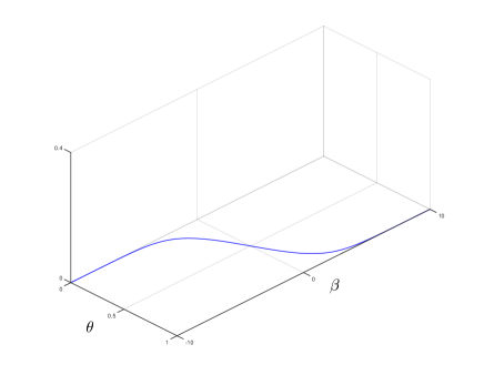
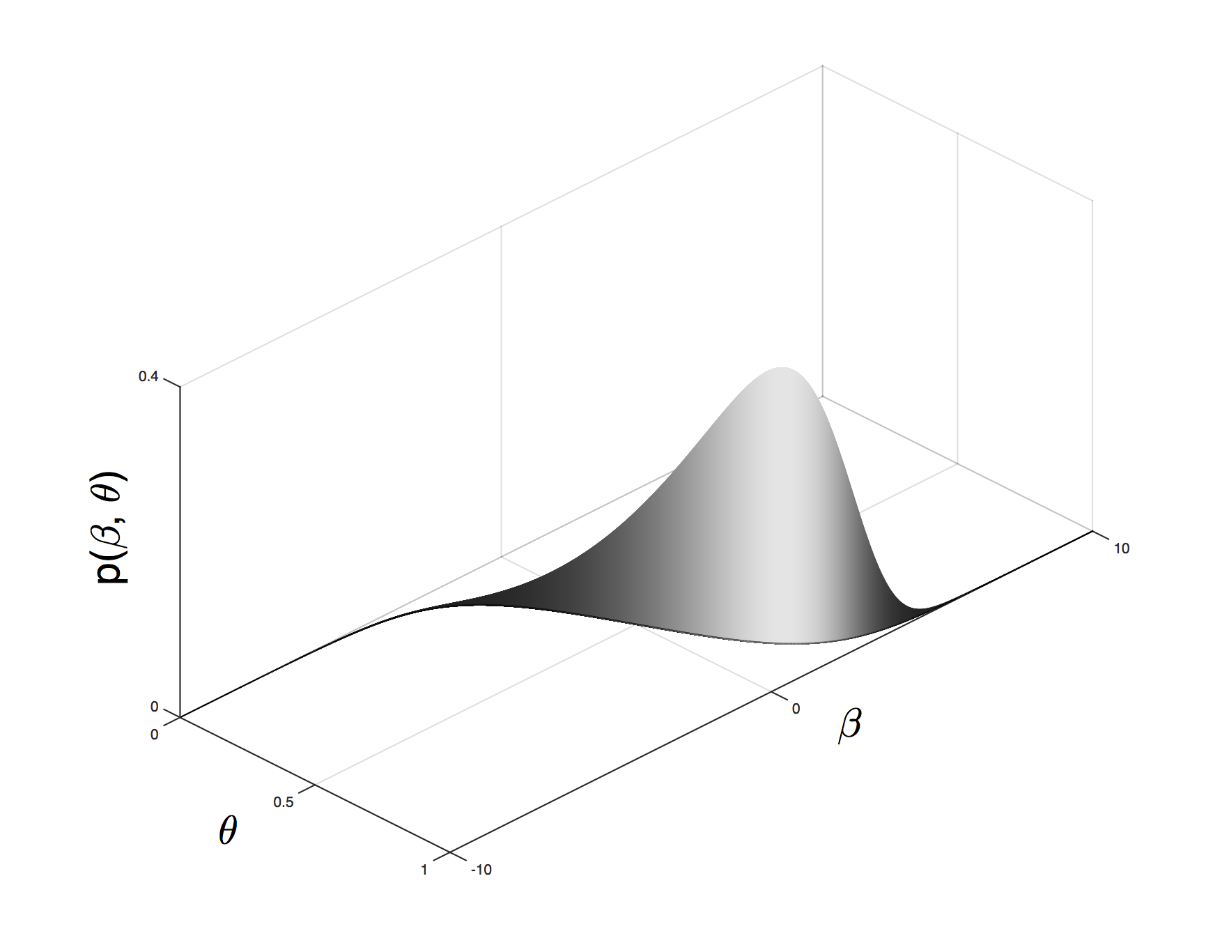
Figure 1: In the plot on the left the blue curve, $\beta=\log\left(\frac{\theta}{1-\theta}\right)$, is the parameter space of the logit model, $\Theta_{\beta,\theta}$. In the plot on the right the density of the prior $p(\beta,\theta)$ (with respect to Hausdorff measure) is depicted. This density lives on the blue curve which supports $\Theta_{\beta,\theta}$.

Of fundamental importance is that if $\theta$ moves by $\mathrm{d}\theta$ then the length of the journey along this curve will be (by Pythagoras’s theorem)

$$\mathrm{d}\theta\sqrt{1+J_{\theta}^{2}},\quad J_{\theta}=\frac{\partial\beta}{\partial\theta}=\frac{\partial\log\left(\frac{\theta}{1-\theta}\right)}{\partial\theta}.$$

The right panel of Figure 1 repeats the support but now above it is a (the form of the density is not expositionally important at this point) density $p(\beta,\theta)$ with respect to this curve, or more formally the one dimension Hausdorff measure on $\Theta_{\beta,\theta}$.  Then for any set $C\subset\Theta_{\beta,\theta}$,

$$\Pr\left\{\left(\beta,\theta\right)\in C\right\}=\int_{C_{\theta}}p(\beta,\theta)\sqrt{1+\left(\frac{\partial\beta}{\partial\theta}\right)^{2}}\mathrm{d}\theta,$$

where $C_{\theta}$ is the projection of $C$ on $\theta$’s axis (i.e. we integrate over all values of $\theta$ which imply a $\beta$ such that the pair $\left(\beta,\theta\right)\in C$). This means as we integrate over $\theta$, we must multiply the density on the curve by the length of the curve.

We will study how to transform this prior $p(\beta,\theta)$ into a posterior and simulate from it. This will allow us to learn $\beta$ from the data. As with all Bayesian calculations, it is not trivial to establish a widely acceptable prior $p(\beta,\theta)$. We will return to that very practical issue in Section 4.

Before we leave this section we give a less artful example.

Example 2

(Mean) Let $Z$ be a scalar random variable and $g(s,\beta)=s-\beta$, so $\beta$ is a mean. Then

$$\Theta_{\beta,\theta}=\left\{(\beta,\theta)\ ;\ \sum_{j=1}^{J}\theta_{j}s_{j}=\beta,\ \theta_{j}>0\ \text{ for all }j,\text{ and }\iota^{\prime}\theta<1\ \right\}.$$

Thus $\Theta_{\beta,\theta}$ is a region within a $(J-1)$-dimensional hyperplane in $\mathbb{R}^{J}$. However all elements of this set are not admissible, since $\theta$ should satisfy the probability axioms (elements of $\theta$ should be positive and $1-\iota^{\prime}\theta>0$). Therefore the parameter space $\Theta_{\beta,\theta}$ is a convex subset on the hyperplane. Then if $\theta$ moves by $\mathrm{d}\theta_{1},...,\mathrm{d}\theta_{J-1}$ the area of the corresponding parallelogram on the hyperplane is

$$\mathrm{d}\theta_{1}...\mathrm{d}\theta_{J-1}\sqrt{1+J_{\theta}J_{\theta}^{\prime}},\quad J_{\theta}=\left\{\left(\frac{\partial\beta}{\partial\theta_{1}}\right),...,\left(\frac{\partial\beta}{\partial\theta_{J-1}}\right)\right\},$$

where $\partial\beta/\partial\theta_{j}=s_{j}-s_{J}$, $j=1,2,...,J-1$. So for any measurable set $C\subset\Theta_{\beta,\theta}$,

$$\Pr\left\{\left(\beta,\theta\right)\in C\right\} = \int_{C_{\theta}}p(\beta,\theta)\sqrt{1+\sum_{j=1}^{J-1}\left(\frac{\partial\beta}{\partial\theta_{j}}\right)^{2}}\mathrm{d}\theta=\int_{C_{\theta}}p(\beta,\theta)\sqrt{1+\sum_{j=1}^{J-1}\left(s_{j}-s_{J}\right)^{2}}\mathrm{d}\theta$$

$$\propto \int_{C_{\theta}}p(\beta,\theta)\mathrm{d}\theta.$$

where $C_{\theta}$ is the projection of $C$ on $\theta$ (The last proportionality is due to the fact that the Jacobian only depends on the support of the data). Thus the linearity of the moment condition (that results in a flat parameter space $\Theta_{\beta,\theta}$) translates into a somewhat trivial multiplicative correction factor and so yields a simple relationship between $\Pr\left\{\left(\beta,\theta\right)\in C\right\}$ and $p(\beta,\theta)$.

Example 3

(Regression) The previous example can be generalized to the family of regression models. For instance consider a linear regression model, $\mathbb{E}\left(s^{(1)}|s^{(2)}\right)=\beta^{\prime}s^{(2)}$, where $s=(s^{(1)},s^{(2)})$, in which $s^{(1)}$ is a scalar and $s^{(2)}$ is a $d$-dimensional vector, and $\beta$ is a $p$-dimensional vector of parameters. The linear regression parameters solve the following moment condition equation,

$$\mathbb{E}\left[g(s,\beta)\right]=\mathbb{E}\left[s^{(2)}(s^{(1)}-\beta^{\prime}s^{(2)})\right]=0.$$

We can also discuss the estimation of linear regression model with instrumental variables. Assume $s=(s^{(1)},s^{(2)},s^{(3)})$, where $s^{(1)}$ is a scalar, and $s^{(2)}$ and $s^{(3)}$ are $p$-dimensional vectors (independent and instrumental variables, respectively). If we define $g(s,\beta)=s^{(3)}(s^{(1)}-\beta^{\prime}s^{(2)})$, then $\beta$ is the solution to $\mathbb{E}\left[g(s,\beta)\right]=0$. Moreover generalizing to the nonlinear regression model is easy. Assume $\mathbb{E}\left(s^{(1)}|s^{(2)}\right)=\mu(s^{(2)},\beta)$. Then the corresponding moment condition equation is $g(s,\beta)=s^{(2)}\left\{s^{(1)}-\mu(s^{(2)},\beta)\right\}$. For instance for a Poisson regression $g(s,\beta)=s^{(2)}\left\{s^{(1)}-\exp(\beta^{\prime}s^{(2)})\right\}$.

Example 4

(Average treatment effect) Consider a casual inference problem with the observational data $Z_{j}=(X_{j},Y_{j},W_{j})$ (for $1\leq j\leq N$), where $X_{j}$ is the $K$-dimensional vector of the $j$-th unit’s background variables, $Y_{j}$ is its scalar outcome variable, and $W_{j}$ is the binary treatment indicator. Assuming the super-population unconfoundedness, it can be shown that (Imbens and Rubin (2015)) $\mathbb{E}_{SP}\left[Y_{j}(1)\right]=\mathbb{E}\left[\frac{W_{j}Y_{j}}{e(X_{j})}\right]$ and $\mathbb{E}_{SP}\left[Y_{j}(0)\right]=\mathbb{E}\left[\frac{(1-W_{j})Y_{j}}{1-e(X_{j})}\right]$, where $e(X_{j})$ is the propensity score, $e(X_{j})=\eta_{j}=\Pr(W_{j}=1|X_{j})$. Therefore the average treatment effect (ATE) is

$$\tau=\mathbb{E}_{SP}\left[Y_{j}(1)\right]-\mathbb{E}_{SP}\left[Y_{j}(0)\right]=\mathbb{E}\left(\frac{W_{j}Y_{j}}{e(X_{j})}-\frac{(1-W_{j})Y_{j}}{1-e(X_{j})}\right),$$

One might use a logistic regression model for the propensity score, $\eta_{j}=\exp(\gamma^{\prime}X_{j})/\left\{1+\exp(\gamma^{\prime}X_{j})\right\}$, where $\gamma$ is $K$-dimensional. Under these assumptions the model’s parameters, $\beta=(\gamma,\tau)$, solve the following set of moment conditions,

$$\mathbb{E}\left[g(Z_{j},\beta)\right]=\mathbb{E}\left[\begin{array}[]{c}X_{j}(Y_{j}-\eta_{j})\\ \frac{(W_{j}-\eta_{j})Y_{j}}{\eta_{j}\left(1-\eta_{j}\right)}-\tau\\ \end{array}\right]=0,$$

If we assume the data points are i.i.d. realizations from a discrete distribution with finite and known support $S=\{s_{1},...,s_{j}\}$, $\Pr(Z_{i}=s_{j})=\theta_{j}$, the moment conditions are,

$$\mathbb{E}\left[g(Z_{j},\beta)\right]=\left[\begin{array}[]{c}\sum_{j=1}^{J}\theta_{j}X_{j}(Y_{j}-\eta_{j})\\ \sum_{j=1}^{J}\theta_{j}\frac{(W_{j}-\eta_{j})Y_{j}}{\eta_{j}\left(1-\eta_{j}\right)}-\tau\end{array}\right]=0.$$

Thus the propensity scores and the ATE can be estimated jointly (e.g. McCandless et al. (2009), Zigler et al. (2013) and Zigler and Dominici (2014)).

3 Inference 

3.1 Likelihood and posterior

Under the assumptions formulated above, the model’s likelihood is

$$L(Z|\beta,\theta)\propto\prod_{j=1}^{J}\theta_{j}^{n_{j}},$$

where $n_{j}=\sum_{i=1}^{N}1(Z_{i}=s_{j})$. Note that although $\beta$ does not appear in the likelihood explicitly, due to the constraints on $\beta$ and $\theta$, the data is informative about $\beta$.

The posterior is supported on the same set as the prior, $\Theta_{\beta,\theta}$, and may be written as

$$p(\beta,\theta|Z)\propto p(\beta,\theta)\left(\prod_{j=1}^{J}\theta_{j}^{n_{j}}\right).$$ (4)

The terms in (4) are easy to compute for any $\left(\beta,\theta\right)$ in $\Theta_{\beta,\theta}$, but the support is defined implicitly.

3.2 Accessing the posterior

Inference can be carried out by sampling from the posterior distribution of the parameters. However, in this problem, traditional simulation algorithms will fail because the prior and the posterior of the model are supported on a zero Lebesgue measure set (e.g. all the proposed moves of a Metropolis-Hastings (MH) algorithm with a traditional proposal will be rejected almost surely).

Here two solutions to this problem are given. In the first approach, called the “marginal method”, we will derive the density function of the marginal of $\theta$, which has a density with respect to the Lebesgue measure $p(\theta)$ and therefore can be processed by conventional Monte Carlo methods. Examples include standard MCMC algorithm and importance sampling. This is simple but comes at the cost of having to solve for $\beta$ for each proposal. If finding $\beta$ (or indeed all the values of $\beta$ which solve given $\theta$) is cheap then this provides a very solid solution to the problem.

In the second approach, called the “joint method”, we define a proposal in the space of $(\beta,\theta)$ that assigns positive probability to $\Theta_{\beta,\theta}$ (so, with positive probability, the proposed moves remain on the manifold $\Theta_{\beta,\theta}$ and will be accepted). An MH algorithm with this proposal is able to efficiently move in the space. This does not require us to solve the moment conditions at all, which is extremely attractive for difficult to solve moment condition models.

3.3 Marginal method

Let $p(\beta,\theta)$ be the density function of the model’s prior or posterior with respect to Hausdorff measure on $\Theta_{\beta,\theta}$. Proposition 1 gives the marginal density of $\theta$ with respect to Lebesgue measure.  This implies that standard Monte Carlo methods (e.g. MCMC, importance sampling, sequential importance sampling and Hamiltonian Monte Carlo) can be used.

Proposition 1

Let $p(\beta,\theta)$ be the density function of the prior or posterior with respect to Hausdorff measure supported on $\Theta_{\beta,\theta}$. Moreover, assume $p=r$ (the “just identified” case) and $\beta$ is uniquely determined by $\theta$, i.e. $\beta=\beta(\theta)$. Then the density function of $\theta$ with respect to Lebesgue measure is

$$p(\theta)=\sqrt{\left|J_{\theta}J_{\theta}^{\prime}+I_{p}\right|}\ p(\beta,\theta),$$ (5)

where

$$J_{\theta}=\frac{\partial\beta}{\partial\theta^{\prime}}=-\left\{\mathbb{E}_{\theta}\left(\frac{\partial g}{\partial\beta^{\prime}}\right)\right\}^{-1}H_{\beta},\quad\text{where\quad}H_{\beta}=\left(g_{1},...,g_{J-1}\right)-g_{J}\iota^{\prime},$$ (6)

with $\iota$ being a $(J-1)$-vector of ones and

$$\mathbb{E}_{\theta}\left(\frac{\partial g}{\partial\beta^{\prime}}\right)=\sum_{j=1}^{J}\theta_{j}\frac{\partial g(s_{j},\beta)}{\partial\beta^{\prime}}.$$

This proposition is a direct result of the “area formula” of Federer (1969) (see also Diaconis et al. (2013)) and it can be generalized straightforwardly to the cases where for some values of $\theta$ there exist more than one $\beta$ by summing over the right hand side for each solution in $\beta$.

The Jacobian term $\sqrt{\left|J_{\theta}J_{\theta}^{\prime}+I_{p}\right|}$ depends on the geometry of the parameter space $\Theta_{\beta,\theta}$ (in other words, it only depends on the moment conditions) and is independent of $p(\beta,\theta)$. To compute this term we need to invert a $p\times p$ matrix and evaluate the determinant of a $p\times p$ matrix. However, $p$ is usually small, in which case the computational cost of these operations is negligible.

Importantly knowledge of the functional form of $\beta$ as a function of $\theta$ is not needed, since the partial derivatives can be obtained by the implicit function theorem. However, in order to evaluate this density function for a given $\theta$, we need its corresponding $\beta$. Although in some problems $\beta$ has a known analytic form as a function of $\theta$, in many other situations it can be obtained through a numeric optimization. We now return to the examples introduced in Section 2.

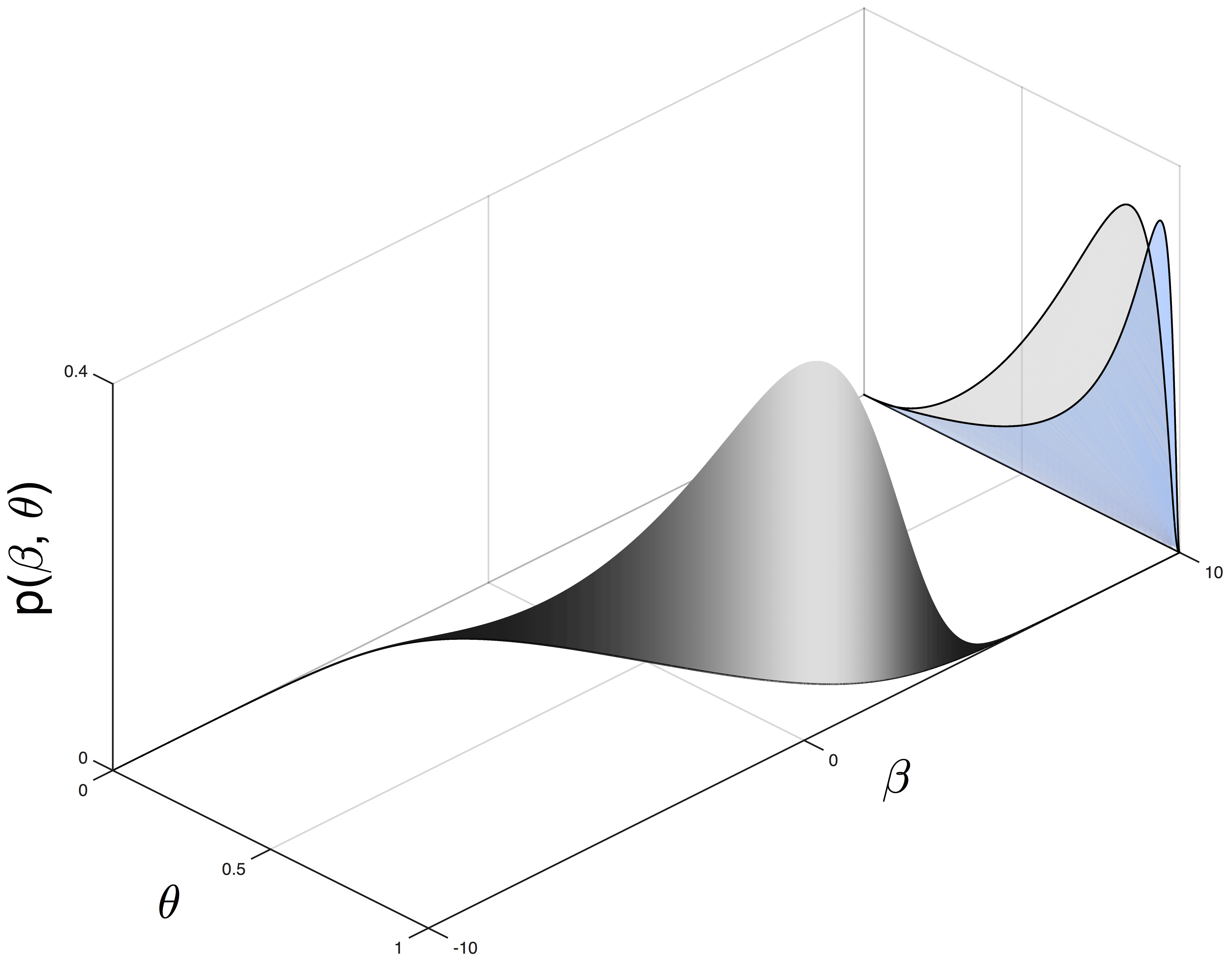
Figure 2: Projection to the marginal density for $\theta$. Blue density is the correct marginal density $p(\theta)$, given in (7), with respect to Lebesgue measure. The grey density is the naive density $p\left[\beta=\log\left\{\theta/\left(1-\theta\right)\right\},\theta\right]$ which ignores the corresponding length of the support.

Example 5 (continues=exa:ExampleLogit1)

The density of $\theta$ in the logistic model is

$$p(\theta)=p(\beta,\theta)\sqrt{1+\left(\frac{\partial\log\left(\frac{\theta}{1-\theta}\right)}{\partial\theta}\right)^{2}}.$$ (7)

Thus moment condition impacts the marginal prior on $\theta$. Figure 2 shows the function $p(\theta)$, which has blue shade below the curve, together with the naive $p\left(\beta=\log\left\{\theta/\left(1-\theta\right)\right\},\theta\right)$, which has grey shade. We can see the correct density is higher for high values of $\theta$ as there are more dense values of $\beta$ compatible with high values of $\theta$ than when $\theta$ is close to 0.5.

Example 6 (continues=exa:ExampleMeanJ3)

The density of $\theta$ in the mean model is

$$p(\theta)=p(\beta,\theta)\sqrt{1+\sum_{j=1}^{J-1}\left(s_{j}-s_{J}\right)^{2}}\ \propto p(\beta,\theta).$$

Hence in this case the geometry of moment condition does not impact the prior on $\theta$. This will be the case generally when the parameter space, $\Theta_{\beta,\theta}$, is flat.

Example 7 (continues=exa:Regression)

For the regression model write $g_{j}=g(s_{j},\beta)$ for $1\leq j\leq J$. Therefore

$$\frac{\partial g_{j}}{\partial\beta^{\prime}}=-s_{j}^{(2)}s_{j}^{(2)\prime},\quad\text{and\quad}\frac{\partial\beta}{\partial\theta_{i}}=\left(\sum_{j=1}^{J}\theta_{j}s_{j}^{(2)}s_{j}^{(2)\prime}\right)^{-1}\left(g_{i}-g_{J}\right).$$

Moreover

$$J_{\theta}J_{\theta}^{\prime}=\left(\sum_{j=1}^{J}\theta_{j}s_{j}^{(2)}s_{j}^{(2)\prime}\right)^{-1}\left\{\sum_{i=1}^{J}\left(g_{i}-g_{J}\right)\left(g_{i}-g_{J}\right)^{\prime}\right\}\left(\sum_{j=1}^{J}\theta_{j}s_{j}^{(2)}s_{j}^{(2)\prime}\right)^{-1}.$$

Similarly for the linear regression model with instrumental variables we have,

$$\frac{\partial g_{j}}{\partial\beta^{\prime}}=-s_{j}^{(3)}s_{j}^{(2)\prime},\quad\text{and\quad}\frac{\partial\beta}{\partial\theta_{i}}=\left(\sum_{j=1}^{J}\theta_{j}s_{j}^{(3)}s_{j}^{(2)\prime}\right)^{-1}\left(g_{i}-g_{J}\right),$$

and therefore

$$J_{\theta}J_{\theta}^{\prime}=\left(\sum_{j=1}^{J}\theta_{j}s_{j}^{(3)}s_{j}^{(2)\prime}\right)^{-1}\left\{\sum_{i=1}^{J}\left(g_{i}-g_{J}\right)\left(g_{i}-g_{J}\right)^{\prime}\right\}\left(\sum_{j=1}^{J}\theta_{j}s_{j}^{(3)}s_{j}^{(2)\prime}\right)^{-1}.$$

Again generalizing to nonlinear regression models is straightforward. If we define $\mu_{j}=\mu(\beta,s_{j}^{(2)})$, then

$$\frac{\partial g_{j}}{\partial\beta^{\prime}}=-s_{j}^{(2)}\frac{\partial\mu_{j}}{\partial\beta^{\prime}},\quad\text{and\quad}\frac{\partial\beta}{\partial\theta_{i}}=\left(\sum_{j=1}^{J}\theta_{j}s_{j}^{(2)}\frac{\partial\mu_{j}}{\partial\beta^{\prime}}\right)^{-1}\left(g_{i}-g_{J}\right),$$

which implies

$$J_{\theta}J_{\theta}^{\prime}=\left(\sum_{j=1}^{J}\theta_{j}s_{j}^{(2)}\frac{\partial\mu_{j}}{\partial\beta^{\prime}}\right)^{-1}\left\{\sum_{i=1}^{J}\left(g_{i}-g_{J}\right)\left(g_{i}-g_{J}\right)^{\prime}\right\}\left(\sum_{j=1}^{J}\theta_{j}s_{j}^{(2)}\frac{\partial\mu_{j}}{\partial\beta^{\prime}}\right)^{-1}.$$

For instance for $\mu(\beta,s^{(2)})=\exp(\beta^{\prime(2)})$ we have,

$$\frac{\partial g_{j}}{\partial\beta^{\prime}}=-s_{j}^{(2)}\exp(\beta_{j}^{\prime(2)})s_{j}^{(2)^{\prime}},\quad\text{and\quad}\frac{\partial\beta}{\partial\theta_{i}}=\left(\sum_{j=1}^{J}\theta_{j}s_{j}^{(2)}\exp(\beta_{j}^{\prime(2)})s_{j}^{(2)^{\prime}}\right)^{-1}\left(g_{i}-g_{J}\right),$$

and hence

$$J_{\theta}J_{\theta}^{\prime}=\left(\sum_{j=1}^{J}\theta_{j}s_{j}^{(2)}\exp(\beta_{j}^{\prime(2)})s_{j}^{(2)^{\prime}}\right)^{-1}\left\{\sum_{i=1}^{J}\left(g_{i}-g_{J}\right)\left(g_{i}-g_{J}\right)^{\prime}\right\}\left(\sum_{j=1}^{J}\theta_{j}s_{j}^{(2)}\exp(\beta_{j}^{\prime(2)})s_{j}^{(2)^{\prime}}\right)^{-1}.$$

Example 8 (continues=exa:HTEstimator)

For the casual inference problem write $g_{j}=g(s_{j},\beta)$, for $1\leq j\leq J$. Then

$$\frac{\partial g_{j}}{\partial\beta^{\prime}}=\left[\begin{array}[]{cc}s_{j}^{(1)}\eta_{j}(1-\eta_{j})s_{j}^{(1)^{\prime}}&0_{K\times 1}\\ 0_{1\times K}&-1\\ &\end{array}\right],\quad\text{and\quad}\frac{\partial\beta}{\partial\theta_{i}}=\left(\left[\begin{array}[]{cc}\sum_{j=1}^{J}\theta_{j}s_{j}^{(1)}\eta_{j}(1-\eta_{j})s_{j}^{(1)^{\prime}}&0_{K\times 1}\\ 0_{1\times K}&-1\\ &\end{array}\right]\right)^{-1}\left(g_{i}-g_{J}\right),$$

which implies

$$J_{\theta}J_{\theta}^{\prime} = \left(\left[\begin{array}[]{cc}\sum_{j=1}^{J}\theta_{j}s_{j}^{(1)}\eta_{j}(1-\eta_{j})s_{j}^{(1)^{\prime}}&0_{K\times 1}\\ 0_{1\times K}&-1\\ &\end{array}\right]\right)^{-1}\left\{\sum_{i=1}^{J}\left(g_{i}-g_{J}\right)\left(g_{i}-g_{J}\right)^{\prime}\right\}$$ (15)

$$\left(\left[\begin{array}[]{cc}\sum_{j=1}^{J}\theta_{j}s_{j}^{(1)}\eta_{j}(1-\eta_{j})s_{j}^{(1)^{\prime}}&0_{K\times 1}\\ 0_{1\times K}&-1\\ &\end{array}\right]\right)^{-1}.$$

An immediate consequence of Proposition 1 is that if we reparametrize the scientific parameters of interest $\psi=\psi(\beta)$ using a one to one transform, then

$$p(\psi,\theta)=\frac{\sqrt{\left|\frac{\partial\beta}{\partial\theta^{\prime}}\frac{\partial\beta}{\partial\theta^{\prime}}^{\prime}+I_{p}\right|}}{\sqrt{\left|\frac{\partial\psi}{\partial\theta^{\prime}}\frac{\partial\psi}{\partial\theta^{\prime}}^{\prime}+I_{p}\right|}}p(\beta,\theta),$$ (16)

where $p(\psi,\theta)$ and $p(\beta,\theta)$ are densities with respect to Hausdorff measures.

3.4 Joint method

Alternatively, we may draw random samples directly from the posterior of $(\beta,\theta)$. This distribution is supported on a zero Lebesgue measure set, $\Theta_{\beta,\theta}$, with the density function (with respect to Hausdorff measure) $p(\beta,\theta)$. If we ignore this and propose moves from a continuous proposal distribution in $\mathbb{R}^{J+p-1}$ (for instance a Gaussian proposal), the proposed moves are off the support of $p(\beta,\theta)$ almost surely, and they will be rejected with probability one. Therefore in order to sample from $p(\beta,\theta)$ we must find a proposal distribution that assigns positive probability to $\Theta_{\beta,\theta}$. Drawing random samples from this proposal should be easy and fast and (in order to compute the acceptance probability) we should be able to evaluate its density function. This subsection will explain how this can be achieved.

For a given value of $\beta$, the moment conditions imply the affine constraints on $\theta$:

$$H_{\beta}\theta+g_{J}=0.$$ (17)

Therefore $\Theta_{\theta|\beta}$ is a $(J-1)$-hyperplane in $\mathbb{R}^{J+p-1}$. This property allows us to define a suitable proposal distribution for $(\beta,\theta)$. Assume the current state of the MCMC is $(\beta^{(t)},\theta^{(t)})$. First we explain how a random sample from the proposal can be drawn, and then will show how the density of this proposal can be evaluated. In order to draw a random sample from $q(\cdot,\cdot|\beta^{(t)},\theta^{(t)})$,

1. Draw $\beta^{*}|\beta^{(t)},\theta^{(t)}$ from an (almost) arbitrary proposal $q(\cdot|\beta^{(t)},\theta^{(t)})$.

2. Draw $\theta^{\ast}$ from a singular distribution supported on the hyperplane $\mathcal{P}^{\ast}=\{\lambda\in\mathbb{R}^{J-1};H_{\beta^{\ast}}^{\ast}\lambda+g_{J}^{\ast}=0\}$. We denote the density of this distribution (with respect to the Hausdorff measure) by $q(\cdot|\beta^{(t)},\theta^{(t)},\beta^{\ast})$. Moreover we assume the density can be easily evaluated at any $\theta^{\ast}$. A singular Normal distribution supported on $\mathcal{P}^{\ast}$ is one suitable choice (see Khatri (1968)). In the Appendix A.3 we provide a way to determine the parameters of a singular Normal distribution that can be used to propose for $\theta^{\ast}|\beta^{(t)},\theta^{(t)},\beta^{\ast}$.

So far we have shown how a random proposal can be generated from $q(\cdot,\cdot|\beta^{(t)},\theta^{(t)})$. The following propositions demonstrates how the density of this proposal can be evaluated when $p=r$.

Proposition 2

Let $p(\beta,\theta)$ be the density of $(\beta,\theta)$ with respect to $(J-1)$-dimensional Hausdorff measure on $\Theta_{\beta,\theta}$. Moreover assume the density of $\beta$ with respect to Lebesgue measure is $p(\beta)$, and the density of $\theta|\beta$ with respect to Hausdorff measure is $p(\theta|\beta)$ on $\Theta_{\theta|\beta}$, where $\Theta_{\theta|\beta}$ is a hyperplane. Then

$$p(\beta,\theta)=\frac{\left|J_{\theta}J_{\theta}^{\prime}\right|^{\frac{1}{2}}}{\left|J_{\theta}J_{\theta}^{\prime}+I_{p}\right|^{\frac{1}{2}}}\ p(\beta)p(\theta|\beta),\quad\text{where\quad}J_{\theta}=\frac{\partial\beta}{\partial\theta^{\prime}}.$$ (18)

The proposed pairs $(\beta^{\ast},\theta^{\ast})$ satisfy the moment conditions, however the probabilities may not satisfy the probability axioms (as some of $\theta^{\ast}$ may be negative or $\theta_{J}^{\ast}=1-\iota^{\prime}\theta^{\ast}\leq 0$). Obviously in these cases the proposal is rejected (since the posterior is zero), the MCMC algorithm sticks, and the proposal’s density need not to be evaluated. If the proposal is valid, then the move $(\beta,\theta)\rightarrow(\beta^{\ast},\theta^{\ast})$ is accepted with probability

$$\min\left\{1,\frac{p(\beta^{\ast},\theta^{\ast}|Z)}{p(\beta,\theta|Z)}\frac{q(\beta,\theta|\beta^{\ast},\theta^{\ast})}{q(\beta^{\ast},\theta^{\ast}|\beta,\theta)}\right\}.$$ (19)

The terms inside this acceptance probability are straightforward to compute up to proportionality.

Note that in the joint method we do not need to solve for $\beta$ in each iteration of the simulation, because our proposed moves are elements of the parameter space $\Theta_{\beta,\theta}$. Moreover, when $J$ goes to infinity, the Jacobian term in (18) converges to $1$. To see this assume the data generating process is a continuous distribution or a discrete distribution with infinite support, $s_{j}\sim H$. Then, with probability one, just using a strong law of large numbers,

$$\frac{1}{J}J_{\theta}J_{\theta}^{\prime}=\frac{1}{J}\left\{\mathbb{E}_{\theta}\left(\frac{\partial g}{\partial\beta^{\prime}}\right)\right\}^{-1}H_{\beta}H_{\beta}^{\prime}\left\{\mathbb{E}_{\theta}\left(\frac{\partial g}{\partial\beta^{\prime}}\right)^{\prime}\right\}^{-1}\rightarrow\mathcal{J}.$$

where $\mathcal{J=}\left\{\mathbb{E}_{\theta}\left(\frac{\partial g}{\partial\beta^{\prime}}\right)\right\}^{-1}\mathbb{E}_{H}(g_{j}g_{j}^{\prime})\left\{\mathbb{E}_{\theta}\left(\frac{\partial g}{\partial\beta^{\prime}}\right)^{\prime}\right\}^{-1}$. Therefore

$$\frac{\left|J_{\theta}J_{\theta}^{\prime}\right|}{\left|J_{\theta}J_{\theta}^{\prime}+I_{p}\right|}=\frac{\left|\frac{1}{J}J_{\theta}J_{\theta}^{\prime}\right|}{\left|\frac{1}{J}J_{\theta}J_{\theta}^{\prime}+\frac{1}{J}I_{p}\right|}\rightarrow 1,$$

with probability one as $J$ goes to infinity. This asymptotic approximation could be used to simplify the computation of the acceptance probability, but otherwise does not change the substance of this section, as proposals will be made in the same way — directly on the manifold.

3.5 Relationship to the Bayesian bootstrap

The Rubin (1981) “Bayesian bootstrap” is at the core of Chamberlain and Imbens (2003).  We can implement our Proposition 1 by using their Bayesian bootstrap as a proposal which can be reweighted to allow for informative priors on $\beta$. Throughout we assume $\beta$ can be solved given $\theta$.

Our generalization of Chamberlain and Imbens (2003) starts with the Dirichlet prior $\pi^{\ast}(\theta)\propto\prod_{j=1}^{J}\theta_{j}^{\alpha-1}$, $\alpha>0$. The Bayesian bootstrap then simulates from the proposal density,

$$g(\theta|Z)\propto\prod_{j=1}^{J}\theta_{j}^{n_{j}+\alpha-1}.$$ (20)

We assume the researcher does this $M$ times, writing the draws as $\left\{\theta^{(k)}\right\}_{k=1,2,...,M}$.  For each $\theta^{(k)}$ we assume there is a unique $\beta^{(k)}$ which solves the corresponding moment conditions. Chamberlain and Imbens (2003) stop at this point, using this sample as a Monte Carlo estimate of the posterior.

Correcting for the geometry of the problem, the actual posterior is

$$p(\theta|Z)\propto p(\beta,\theta)\left(\prod_{j=1}^{J}\theta_{j}^{n_{j}}\right)\left|J_{\theta}J_{\theta}^{\prime}+I_{p}\right|^{\frac{1}{2}}.$$ (21)

The resulting weights from the true posterior density with respect to the Lebesgue measure dividing by the density from the proposal are

$$w^{(k)}=\frac{p(\beta^{(k)},\theta^{(k)})\left|J_{\theta}^{(k)}J_{\theta}^{(k)^{\prime}}+I_{p}\right|^{\frac{1}{2}}}{\prod_{j=1}^{J}\left(\theta_{j}^{(k)}\right)^{\alpha-1}},\quad k=1,2,...,M,$$ (22)

(where $J_{\theta}^{(k)}$ is equal to $J_{\theta}$ evaluated at $(\beta^{(k)},\theta^{(k)})$) which normalize as $w^{(k)^{\ast}}=w^{(k)}/\left(\sum_{k=1}^{M}w^{(k)}\right)$. An encouraging aspect of this weight is that it does not depend on the data.

In the special case where $p(\beta,\theta)\propto\pi(\beta)\pi^{\ast}(\theta)$, the weights may be simply evaluated as

$$w^{(k)}\propto\pi(\beta^{(k)})\left|J_{\theta}^{(k)}J_{\theta}^{(k)^{\prime}}+I_{p}\right|^{\frac{1}{2}},\quad k=1,2,...,M.$$ (23)

We can use these weights to estimate $\mathrm{E}\left(h(\beta)|Z\right)\simeq\frac{1}{M}\sum_{k=1}^{M}w^{(k)^{\ast}}h(\beta^{(k)})$. This is importance sampling, e.g. Marshall (1956), Geweke (1989), Liu (2001). An alternative is to resample with probability proportional to the weight $w^{(k)}$, which delivers sampling importance resampling (SIR, see Rubin (1988)). As with all importance samplers, the weights may become uneven although the simplicity of the structure of the weights is encouraging. This sampling strategy becomes appealing in the models where the $\beta$ can be computed easily for any $\theta$, and the prior distribution of $\beta$ is not too far from the posterior obtained from the Bayesian bootstrap.

3.6 Missing support

So far we have assumed the support of the data is known. Here we extend this to assume the support has $J^{\ast}>J$ elements, $S^{\ast}=(s_{1},...,s_{J^{\ast}})$, where its first $\tilde{J}=J^{\ast}-J$ elements, $\tilde{S}=(s_{1},...,s_{\tilde{J}})$, have not been observed in the sample, while the rest of its elements $S=(s_{\tilde{J}+1},...,s_{J})$ have been observed at least once. Moreover let $\theta^{\ast}=(\tilde{\theta},\theta)$, where $\tilde{\theta}$ and $\theta$ are the vector of the probabilities of the elements of $\tilde{S}$ and $(s_{\tilde{J}+1},...,s_{J-1})$, and define $\theta_{J^{\ast}}=1-\sum_{j=1}^{J^{\ast}-1}\theta_{j}^{\ast}$. We assume the missing elements of the support are i.i.d. draws from $F_{S}$, $s_{j}\overset{iid}{\sim}F_{S}$ for $j=1,...,\tilde{J}$, with density $f_{S}$ with respect to Lebesgue measure. The moment conditions are then

$$\sum_{j=1}^{J^{\ast}}\theta_{j}g(s_{j},\beta)=0,$$ (24)

while the posterior is

$$p(\beta,\theta^{\ast},\tilde{S}|Z)\propto p(\beta,\theta^{\ast},\tilde{S})\left(\prod_{j=1}^{J^{\ast}}\theta_{j}^{n_{j}}\right),$$

where $n_{j}=\sum_{i=1}^{N}1(Z_{i}=s_{j})$. Note that $n_{j}=0$ for $1\leq j\leq\tilde{J}$, while $n_{j}$ is positive for $\tilde{J}+1\leq j\leq J^{\ast}$.
Assume the researcher expresses a prior on $(\beta,\theta^{\ast})|\tilde{S}$ with respect to the Hausdorff measure (suppressing the conditioning on $S$ for notational convenience),

$$p(\beta,\theta^{\ast}|\tilde{S}).$$ (25)

Therefore

$$p(\beta,\theta^{\ast},\tilde{S})=\left(\prod_{j=1}^{\tilde{J}}f_{S}(\tilde{s}_{j})\right)p(\beta,\theta^{\ast}|\tilde{S})$$ (26)

Given $\theta^{\ast}$ and $\tilde{S}$ (and $S$), $\beta$ is uniquely determined. Therefore the core result we need to do inference is a generalization of Proposition 1: the density of the probabilities and the missing support with respect to the Lebesgue measure is

$$p(\theta^{\ast},\tilde{S})=\left|J_{\theta^{\ast}}J_{\theta^{\ast}}^{\prime}+J_{\tilde{S}}J_{\tilde{S}}^{\prime}+I_{p}\right|^{\frac{1}{2}}\left(\prod_{j=1}^{\tilde{J}}f_{S}(\tilde{s}_{j})\right)p(\beta,\theta^{\ast}|\tilde{S}),$$ (27)

where

$$J_{\theta^{\ast}} = \frac{\partial\beta}{\partial\theta^{\ast}}=\left(\sum_{j=1}^{J^{\ast}}\theta_{j}\frac{\partial g_{j}}{\partial\beta^{\prime}}\right)^{-1}H_{\beta}^{\ast},\quad J_{\tilde{S}}=\frac{\partial\beta}{\partial\tilde{S}}=\left(\sum_{j=1}^{J^{\ast}}\theta_{j}\frac{\partial g_{j}}{\partial\beta^{\prime}}\right)^{-1}\tilde{M},$$

$$\tilde{M} = \left\{\theta_{1}\left(\frac{\partial g_{1}}{\partial s_{1}^{\prime}}\right),\cdots,\theta_{\tilde{J}}\left(\frac{\partial g_{\tilde{J}}}{\partial s_{\tilde{J}}^{\prime}}\right)\right\}.$$ (28)

Again this result follows from the area formula. Proposition 2 generalizes in the same way delivering

$$p(\beta,\theta^{\ast},\tilde{S})=\frac{\left|J_{\theta^{\ast}}J_{\theta^{\ast}}^{\prime}+J_{\tilde{S}}J_{\tilde{S}}^{\prime}\right|^{\frac{1}{2}}}{\left|J_{\theta^{\ast}}J_{\theta^{\ast}}^{\prime}+J_{\tilde{S}}J_{\tilde{S}}^{\prime}+I_{p}\right|^{\frac{1}{2}}}\ p(\beta)p(\theta^{\ast}|\beta,\tilde{S})\left(\prod_{j=1}^{\tilde{J}}f_{S}(\tilde{s}_{j})\right).$$ (29)

Again the Jacobian will be close to one if $J^{\ast}$ is large.  The ratio of $J$ to $J^{\ast}$ does not make any difference to this approximation.

Example 9 (continues=exa:ExampleMeanJ3)

Now add a single point of missing support.  Then $J^{\ast}=4$, $\theta^{\ast}=\left(\theta_{1},\theta_{2},\theta_{3}\right)^{\prime}$, $J=3$ and $S^{\ast}=\{s_{1},s_{2},s_{3},s_{4}\}=\{-1,0,1,s_{4}\}$. Then $\beta=\theta_{3}-\theta_{1}+s_{4}\theta_{4}=\theta_{3}-\theta_{1}+s_{4}(1-\theta_{1}-\theta_{2}-\theta_{3})$. For this model

$$J_{\theta^{\ast}}=\frac{\partial\beta}{\partial\theta^{\ast}}=\left(-1-s_{4},-s_{4},1-s_{4}\right)\quad\text{and\quad}J_{\tilde{S}}=\frac{\partial\beta}{\partial\tilde{S}}=\theta_{4},$$ (30)

and so $J_{\theta}J_{\theta}^{\prime}=2+3s_{4}^{2}$ and $J_{\tilde{S}}J_{\tilde{S}}^{\prime}=\theta_{4}^{2}$. Hence, writing $\theta_{4}=1-\theta_{1}-\theta_{2}-\theta_{3}$,

$$p(s_{4},\theta^{\ast})=\left\{\sqrt{\left(2+3s_{4}^{2}\right)+\theta_{4}^{2}+1}\right\}f_{S}(s_{4})p(\beta,\theta^{\ast}|s_{4}).$$ (31)

4 Some potential priors

So far we have discussed working with any prior $p(\beta,\theta)$ which is defined with respect to lower dimensional Hausdorff measure supported on $\Theta_{\beta,\theta}$. In this section we discuss potential ways of selecting $p(\beta,\theta)$. As with all prior selection there is no uniquely good way of carrying this out.

4.1 A non-science prior

From a nonparametric standpoint it is natural to build a prior from $p(\theta)$, e.g. Dirichlet.  Then Proposition 1 implies there is a unique joint prior

$$p(\beta,\theta)=\frac{p(\theta)}{\sqrt{\left|J_{\theta}J_{\theta}^{\prime}+I_{p}\right|}},$$ (32)

which achieves this. The right hand side $p(\theta)$ is the density of $\theta$ with respect to Lebesgue measure, while $p(\beta,\theta)$ is the density of $(\beta,\theta)$ with respect to Hausdorff measure.  This implies

$$\Pr\left\{\left(\beta,\theta\right)\in C\right\}=\int_{C_{\theta}}p(\theta)\mathrm{d}\theta.$$ (33)

The Dirichlet special case (32) is the implicit Chamberlain and Imbens (2003) prior on $p(\beta,\theta)$.

4.2 A prior on the science

Proposition 2 says that

$$p(\beta,\theta)=\frac{\left|J_{\theta}J_{\theta}^{\prime}\right|^{1/2}}{\left|J_{\theta}J_{\theta}^{\prime}+I_{p}\right|^{1/2}}p(\beta)p(\theta|\beta).$$ (34)

If we place a prior on the science $p(\beta)$ with respect to the Lebesgue measure, then we can form a scientifically centered prior on $p(\beta,\theta)$ by specifying a prior on $p(\theta|\beta)$ with respect to the $J-1-p$ dimensional Hausdorff measure. This prior sits on the hyperplane $\theta|\beta$ satisfying the linear constraints (17) and the probability axioms.  One such prior is Dirichlet subject to the constraints. Again if $J$ gets large the Jacobian in (34) will become unimportant in practice.

4.3 Adhoc priors

A more brutal approach to building a prior is to define an “initial” prior (with respect to Lebesgue measure) for $\beta$ and $\theta$ which ignores the moment condition $\eta(\beta,\theta)$ where the implied initial marginal prior on $\beta$, $\eta\left(\beta\right)$, could be our substantive initial prior. From the Borel paradox (Kolmogorov (1956)) we know there are many ways of building a $p(\beta,\theta)$ from $\eta(\beta,\theta)$ (conditioning on satisfying the moment condition is not enough) but here we discuss various plausible methods.

This line of thinking leads to a generalization of (32), setting

$$p(\beta,\theta)\propto\frac{\eta(\beta,\theta)}{\left|J_{\theta}J_{\theta}^{\prime}+I_{p}\right|^{1/2}}1_{\Theta_{\beta,\theta}}(\beta,\theta).$$ (35)

This prior scales the initial prior to countereffect the length of the curve mapping out the relationship between $\theta$ and $\beta$ implied by the moment condition.  This prior has the property that $p(\theta)\propto\eta(\beta,\theta)1_{\Theta_{\beta,\theta}}(\beta,\theta)$, with respect to the Lebesgue measure.

The simple case of $\eta(\beta,\theta)=\eta(\beta)\eta(\theta)$, would imply under (35)

$$p(\theta)\propto\eta(\beta)\eta(\theta)1_{\Theta_{\beta,\theta}}(\beta,\theta).$$ (36)

The case where $\eta(\theta)$ is Dirichlet is important. Then the Bayesian bootstrap weights (35) would become the rather simple

$$w_{j}\propto\eta(\beta^{(j)}),\quad j=1,2,...,M.$$ (37)

This is a minimally informative generalization of Chamberlain and Imbens (2003).

Figure 3: The parameter space (the blue curve) $\Theta_{\beta,\theta}$ and the initial prior $\pi(\beta,\theta)$ have been depicted. Figure 1 shows the implied $p(\beta,\theta)$.

An alternative to (35) is to put no mass on inadmissible combinations of $\beta,\theta$. We call this the “truncated prior”

$$p(\beta,\theta)\propto\eta(\beta,\theta)1_{\Theta_{\beta,\theta}}(\beta,\theta)$$ (38)

in which $p(\beta,\theta)$ is the density of the prior with respect to the $(J-1)-$dimension Hausdorff measure in $\mathbb{R}^{J-1+p}$. This would imply for any set $C\in\mathbb{R}^{J-1+p}$

$$\Pr\left\{\left(\beta,\theta\right)\in C\right\} = \int_{C_{\theta}}p(\beta,\theta)\sqrt{\left|J_{\theta}J_{\theta}^{\prime}+I_{p}\right|}\mathrm{d}\theta$$

$$\propto \int_{C_{\theta}}\eta(\beta,\theta)\sqrt{\left|J_{\theta}J_{\theta}^{\prime}+I_{p}\right|}\mathrm{d}\theta.$$

Obviously it implies $p(\theta)\propto\eta(\beta,\theta)\sqrt{\left|J_{\theta}J_{\theta}^{\prime}+I_{p}\right|}1_{\Theta_{\beta,\theta}}(\beta,\theta)$, with respect to the Lebesgue measure.

Example 10

(continuing logistic Example 1).  Assume the initial prior

$$\eta(\beta,\theta)\propto\theta^{0.01-1}(1-\theta)^{0.01-1}e^{-\frac{1}{2}\left(\beta-1\right)^{2}},$$ (40)

which is a relatively ignorant Dirichlet prior on the probabilities and an informative Gaussian prior for $\beta$ centered on one. This is depicted in Figure 3. With this initial prior and using the class of priors (38), the density with respect to the univariate Hausdorff measure is

$$p(\beta,\theta)\propto\eta(\beta,\theta)1_{\Theta_{\beta,\theta}}(\beta,\theta).$$ (41)

Figure 1 shows the corresponding $p(\beta,\theta)$ living on the manifold. In this case

$$p(\theta)\propto\eta(\beta,\theta)\sqrt{1+\left(\frac{\partial\beta}{\partial\theta}\right)^{2}}1_{\Theta_{\beta,\theta}}(\beta,\theta),$$ (42)

with respect to the Lebesgue measure. With the alternative (35) prior, then

$$p(\beta,\theta)\propto\frac{\eta(\beta,\theta)}{\sqrt{1+\left(\frac{\partial\beta}{\partial\theta}\right)^{2}}}1_{\Theta_{\beta,\theta}}(\beta,\theta),\quad\text{and\quad}p(\theta)\propto\eta(\beta,\theta)1_{\Theta_{\beta,\theta}}(\beta,\theta).$$ (43)

5 Illustrative examples

In this section we present some illustrative examples and simulation studies. Since the MCMC results obtained by the marginal and joint methods are indistinguishable we present only one of them. At the end of the section we study how the methods scale.

5.1 The mean

Recall inference on the mean studied in Example 2. Now focus on $J=3$ and $S=(-1,0,1)$, so $\beta=\theta_{3}-\theta_{1}=1-2\theta_{1}-\theta_{2}$. Here we have taken the 2 dimensional Hausdorff prior as

$$p(\beta,\theta)\propto e^{-2\left|\beta-m\right|}\theta_{1}^{\alpha-1}\theta_{2}^{\alpha-1}\left(1-\theta_{1}-\theta_{2}\right)^{\alpha-1}1\left({\min\{\theta_{1},\theta_{2},1-\theta_{1}-\theta_{2}\}\geq 0}\right).$$ (44)

We call this a “Laplace-Dirichlet” distribution on $\left(\beta,\theta\right)$, where $\beta$ is centered around $m$ and the Dirichlet part is indexed by $\alpha$.

By the marginal method:

$$p(\theta)\propto e^{-2\left|1-2\theta_{1}-\theta_{2}-m\right|}\theta_{1}^{\alpha-1}\left(1-\theta_{1}-\theta_{2}\right)^{\alpha-1}\theta_{2}^{\alpha-1}1\left({\min\{\theta_{1},\theta_{2},1-\theta_{1}-\theta_{2}\}\geq 0}\right),$$ (45)

Figure 4 shows the contours of $p(\theta)$ for various values of $m$ and $\alpha$. We have plotted these contours against $\left(\theta_{1},\theta_{2},\theta_{3}\right)^{\prime}$ so the reader can compare $\theta_{1}$ and $\theta_{3}$.

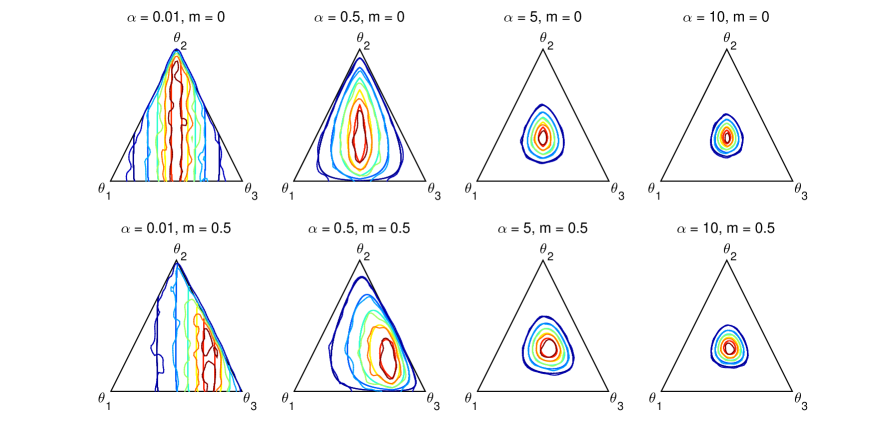
Figure 4: Equiprobability contours implied by the Laplace-Dirichlet prior on $p(\beta,\theta)$ with respect to the Hausdorff measure.  Plotted is the marginal $p(\theta_{1},\theta_{3})$ for several values of $m$ and $\alpha$, with $\theta_{2}$ implied as $\theta_{2}=1-\theta_{1}-\theta_{3}$.  This case has $J=3$ points of support ($s_{1}=-1,s_{2}=0,s_{3}=1$) and $r=1$ moment constraints (the mean).   

If the Laplace-Dirichlet distribution has $m=0$ then the density is symmetric with respect to $\theta_{1}$ and $\theta_{3}$. When the location parameter of $p(\beta)$ is positive $\theta_{1}$ is on average smaller than $\theta_{3}$. Moreover as $\alpha$ increases, the variability of $p(\theta)$ decreases.

Figure 5 draws the prior for $\beta$. Here the support of the data means $\beta$ is restricted to the real line, after observing the support of the data its prior is restricted to $[-1,1]$. As $\alpha$ increases the variance of $\beta$ decreases. For instance the $\beta$’s prior centered at a positive value results in a prior for $\theta$ tilted toward $\theta_{3}$, even if the prior of $\theta$ is symmetric. In the same way, a more informative initial prior for $\theta$ yields a more peaked prior for $\beta$.

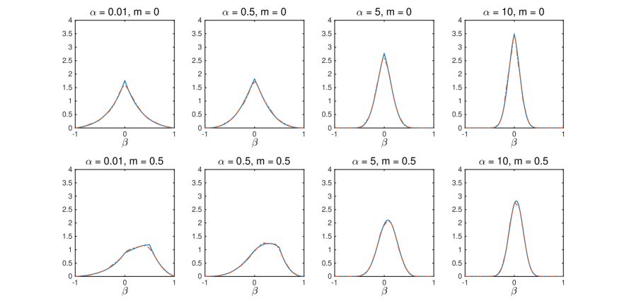
Figure 5: Illustrating Example 1 (estimating the mean). Plot of $p(\beta)$ for several values of $m$ and $\alpha$. This case has $J=3$ points of support ($s_{1}=-1,s_{2}=0,s_{3}=1$) and $r=1$ moment constraints (the mean). Initial prior for $\beta$ is Laplace centered at $m$ and the initial prior for $\theta$ is symmetric Dirichlet with parameter $\alpha$.

5.2 Missing support and the mean

In the previous section, the finite support of $\beta$ is caused by the known support of the data.  We now extend this to cover Example 2 where we have a single missing datapoint

$$s_{4}\sim N(0,10^{2}),$$ (46)

all other features of the problem are unchanged. An adaptive MH algorithm has been used in order to draw $10,000$ samples from the joint distribution. For the sake of brevity we present the results only for the case of $m=0$ and $\alpha=0.5$.

The means and standard error of the probabilities $\theta^{\ast}$ are $(0.3065,0.3335,0.3079,0.0521)$ and $(0.0026,0.0030,0.0024,0.0010)$, respectively. The left panel of Figure 6 shows the initial prior (46) and the implied marginal distribution of the missing element of the support $s_{4}$ from the joint prior. The variance of the implied marginal is smaller than the prior’s variance, because the prior distribution of $\beta$ is informative about the support of the data. The right panel of Figure 6 shows the Laplace element of the prior $e^{-2\left|\beta-m\right|}$ and the full marginal prior for $\beta$.  The full marginal prior is not the same as the Laplace distribution due to the informative priors on the probabilities.

Figure 6: Illustrating Example 1 with the partially observed support: inferring the mean $\beta$. The prior and the posterior of the missing element of the support $s_{4}$ (left panel) and mean $\beta$ (right panel).

5.3 Linear regression

Recall the linear regression of Example 3. Assume the observed data is $Z=\{(1,1),(2,4),(3,9)\}$. Earlier we have seen that the parameter space, $\Theta_{\beta,\theta}$ is a non-flat surface in $\mathbb{R}^{3}$. Figure 7 demonstrates the posterior distribution of the parameters defined on this surface (the prior parameters are $\alpha=0.5$ and $m=3$).

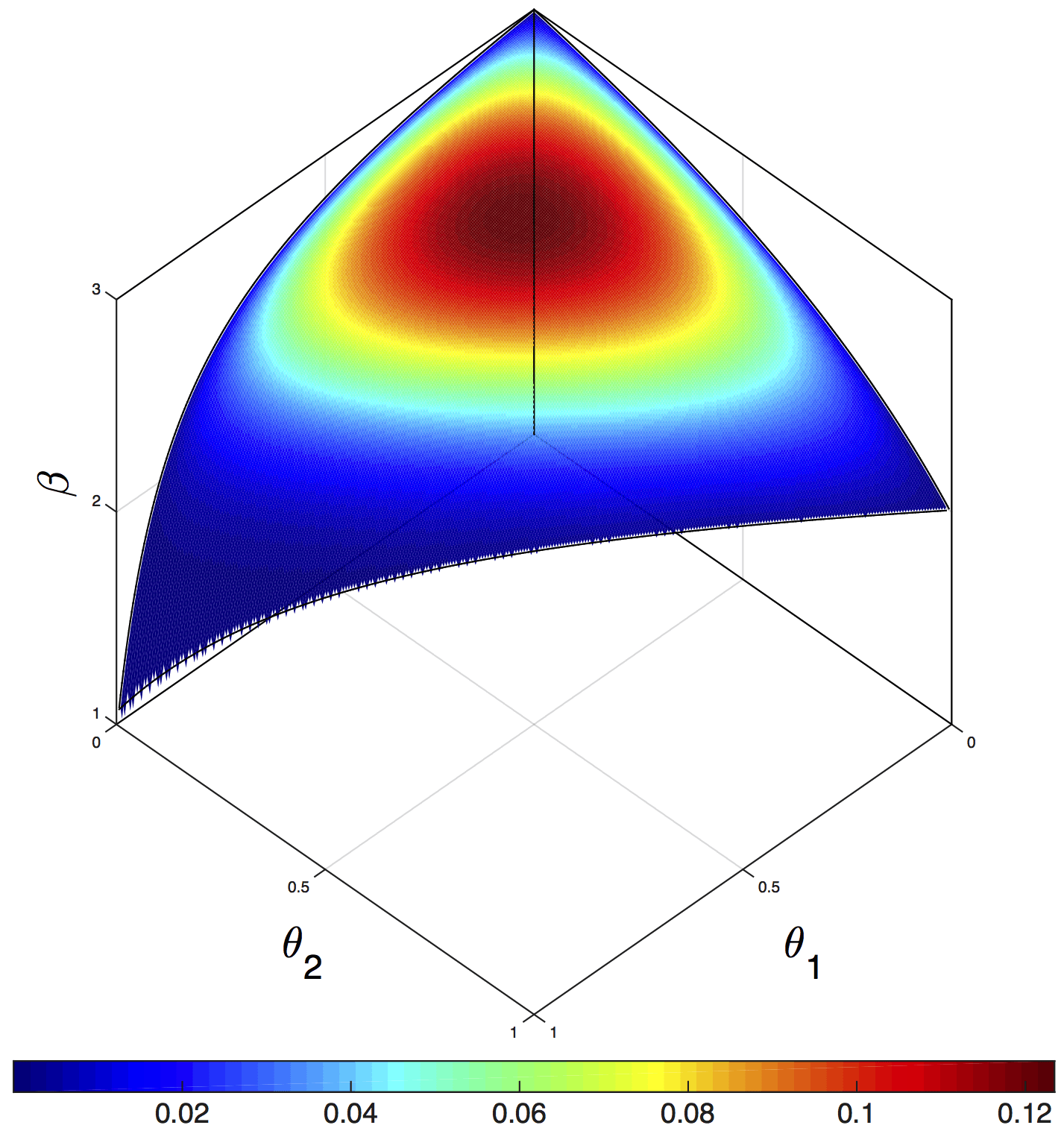
Figure 7: The posterior distribution of the linear regression model with data $Z=\{(1,1),(2,4),(3,9)\}$. The prior parameters are $\alpha=0.5$ and $m=3$.

Following the suggested MCMC simulation algorithms we draw $100,000$ samples from the posterior distribution of the parameters. In the Figure 8 we have drawn the contour plots of the posterior distribution of the probabilities. Analytical results have been compared with the estimates obtained by a kernel density estimator using the MCMC draws.

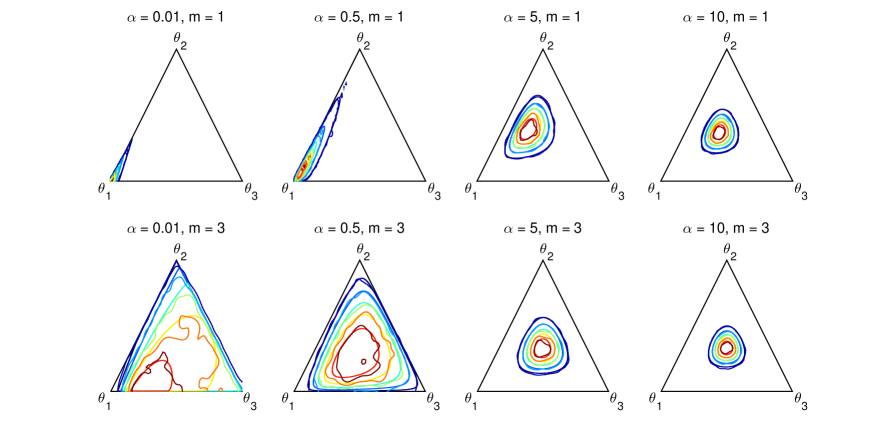
Figure 8: The posterior distribution of $\theta$ in the linear regression model with data $Z=\{(1,1),(2,4),(3,9)\}$ (analytical results and the estimates obtained by a kernel density estimator using $100,000$ MCMC draws). The prior parameters are $\alpha=0.5$ and $m=3$.

5.4 Simulation study

To demonstrate the scalability of the algorithms we consider a linear regression model with sample size $J=500$. The data $Z_{j}=(Y_{j},X_{j})$, for $1\leq j\leq J$, is generated according to $X_{j}\sim\mathcal{N}(1,2^{2})$, $Y_{j}|X_{j}\sim\mathcal{N}(2+5X_{j},10^{2})$.  We assume the substantive prior of $\beta$ is $\beta\sim\mathcal{N}(\mu_{0},\Sigma_{0})$, where the elements of $\mu_{0}$ are equal to the $25\%$ quantiles of the asymptotic MLE estimators, and $\Sigma_{0}$ is equal to the asymptotic variance of the MLE estimator multiplied by $100$ (see Appendix A.5 for the results with a different prior). The initial prior of $\theta$ is a symmetric Dirichlet distribution with parameter $\alpha=0.01$. We have drawn $50,000$ samples from the posterior after a $5,000$ sample burn-in (the chain’s trace has been thinned with a factor of $100$, so has been iterated $5,000,000$ times). The scatter plot of the sample is depicted in the top-left panel of Figure 9. Each circle represents a data point in our sample and its radius is proportional to the expected value of its posterior probability, i.e. $\mathbb{E}(\theta_{j}|Z)$. In the top-right panel the correlogram (ACF) of the chains of $\beta$ and $10$ elements of $\theta$ have been presented (the red dashed lines and the blue dotted lines are corresponding to $\beta$ and $\theta$, respectively.) The ACFs demonstrate that the Markov chain is mixing sufficiently well. In the bottom-left panel the contour plot of the posterior distribution of $\beta$ has been compared to the one obtained by the Bayesian bootstrapping of Chamberlain and Imbens (2003). The posterior distributions are very close, because the prior’s information is roughly $1\%$ of the information content of the sample. The bottom-right panel shows a histogram of the samples from the posterior distribution of $\beta$.

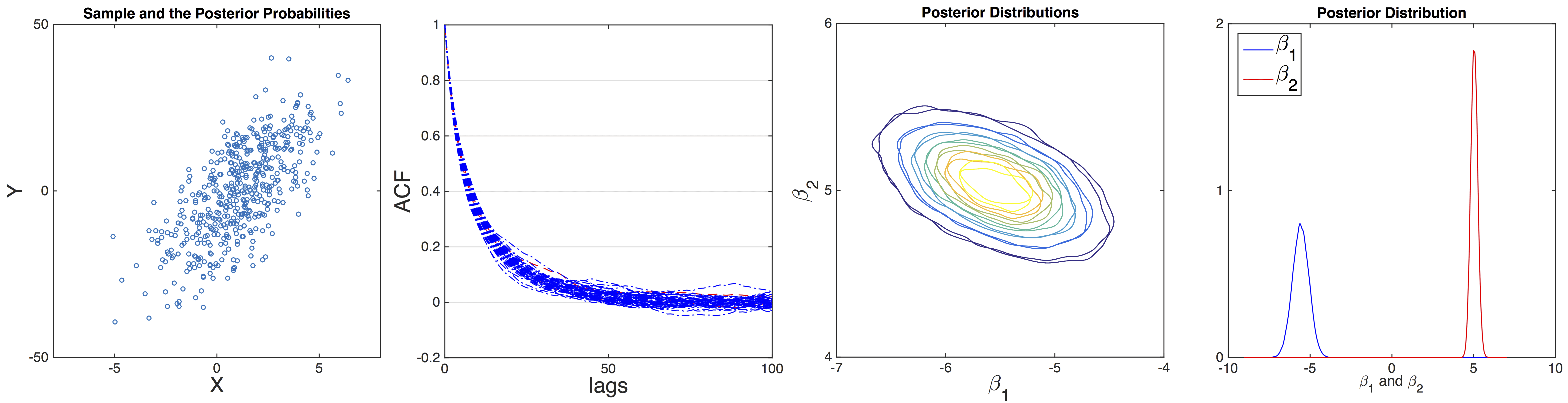
Figure 9: Inference in linear regression model with $J=500$. Top left shows circles who’s radius is the posterior expectation of the probabilities given the data: $E(\theta_{j}|Z)$. Top right is the correlogram for the thinned draws of the elements of $\beta$ and ten elements of $\theta$. The bottom graphs show the estimated contour and marginal densities of the resulting posterior.

6 Empirical studies

In this section we study two empirical examples. The first focuses on an instrumental variable based estimator, the second looks at estimating the average treatment effect from an experiment.

6.1 Instrumental variables

In this section we demonstrate the applicability and scalability of the methodology developed in this paper to a real dataset. We use a subsample of the earnings and schooling dataset studied in Chamberlain and Imbens (2003). This dataset is a subset of the data studied in Angrist and Krueger (1991) and consist of the self-reported weekly log-earnings (self-reported annual earnings divided by 52) of $162,512$ male subjects who reported positive annual wages in 1979 along with their number of years of education and their quarter of birth date. In turn this is a 5% random sample from the 1980 Public Use Census Data.  Bound et al. (2001) discuss the myriad of problems of self-report income data but we do not address that issue here.  For example, Britton et al. (2015) compared UK self-reported income with tax based administrative data finding high income earners significantly under self-recorded their incomes compared to that seen in administrative data.

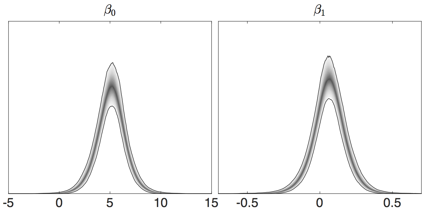
$J=100$

$J=1,000$

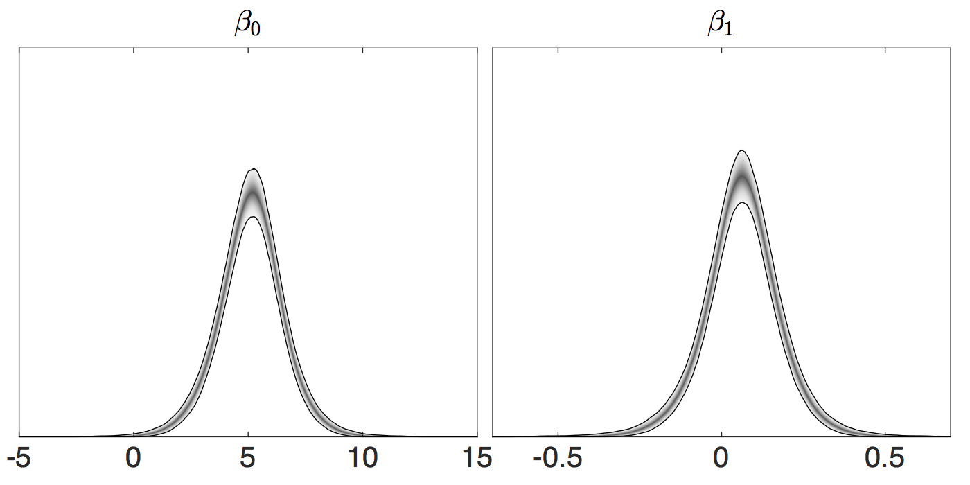
$J=5,000$

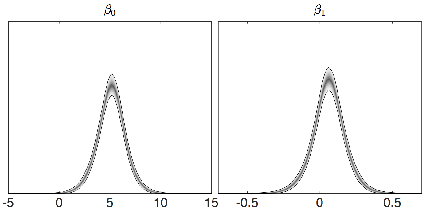
$J=10,000$

Figure 10: 95% pointwise confidence regions for the marginal prior for $\beta$ for $J=10$, $J=1,000$, $J=10,000$ and $J=100,000$ points of random support in top-left, top-right, bottom-left and bottom-right, respectively. The confidence region is computed over 1,000 replications.

Chamberlain and Imbens (2003) studied the dependence of earnings on the level of schooling using a linear additive treatment effect model (e.g. Imbens and Rubin (2015)). They model schooling levels as being determined by rational agents’ optimization of their lifetime expected utility. Since the utility is a function of the earnings they needed to estimate the distribution of earnings as a function of the schooling level.

The expected log-earnings $Y_{X}$ with schooling level $X$ is modeled here as $\mathrm{E}(Y_{X}|X,Y_{0})=Y_{0}+\beta_{1}X$, where $X$ is the schooling level, $\beta_{1}$ is the unknown return to education, and $Y_{0}$ is the earnings level with no schooling at all. Let $\beta_{0}$ be the expected value of $Y_{0}$, so $Y_{0}-\beta_{0}$ has a zero mean.

In order to estimate the unknown parameters, $\beta=(\beta_{0},\beta_{1})$, we follow Angrist and Krueger (1991) and Chamberlain and Imbens (2003) and use an instrumental variable (IV) $W$ that is a binary indicator: $W=0$ if the subject was born in the first three quarters of the year and $W=1$ otherwise. The instrumental variable $W$ is correlated with the regressor $X$ and thought by the researchers to be uncorrelated with the errors.

We obtain the classic IV estimate of $\beta$ using the full sample, and treat them as the “true” values of $\beta$. Then we draw random samples with replacement of size $J$ from the original data $1,000$ times. Our aim will be to compare different estimators using these smaller samples.

Our prior distribution, which is specified to be weakly informative, is

$$p(\beta,\theta)\propto\frac{1}{\sqrt{J_{\theta}J_{\theta}^{\prime}+I_{2}}}\eta(\beta)\eta(\theta)1_{\Theta_{\beta,\theta}}(\beta,\theta),$$ (47)

where $\eta(\beta)=\varphi\left(\beta_{0};5,4\right)\varphi\left(\beta_{1};0,0.2\right)$, and $\varphi\left(\cdot;\mu,\sigma^{2}\right)$ is the Gaussian density with mean $\mu$ and variance $\sigma^{2}$. The intercept is centered at $5$ with variance $4$, implying that the mean annual income for those with no schooling is equal to $\$7,717$ (with $95\%$ confidence interval $[\$153,\$388965]$) with zero years of schooling. Moreover the prior of $\beta_{1}$ has zero mean (no effect of number of schooling years on income) with $95\%$ interval $[-0.88,0.88]$ (that is equivalent to $[-0.41\%,241\%]$ income increment for each additional year of schooling.) The probabilities $\theta$ are taken as a mildly informative Dirichlet prior $\eta(\theta)\propto\mathop{\displaystyle\prod}\limits_{j=1}^{J}\theta_{j}^{\alpha-1}$, where $\alpha=10^{-6}$ (we also tried $\alpha=J^{-1}$, with no substantial change in the results).

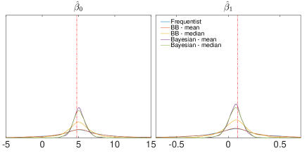
$J=10$

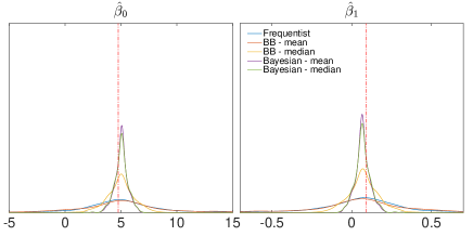
$J=1,000$

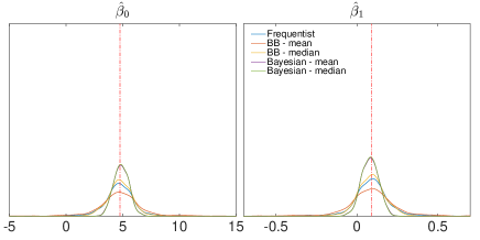
$J=10,000$

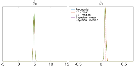
$J=100,000$

Figure 11: The sampling distribution of classic IV (denoted frequentist), Bayesian bootstrapping and Bayesian estimators of $\beta$ in the linear regression model with the instrumental variable employing sample sizes $J=10$, $J=1,000$, $J=10,000$ and $J=100,000$.

For $1,000$ iterations, a random sample of size $J$ has been drawn with replacement from the $162,512$ population. For each replication the resulting marginal prior distributions of $\beta_{0}$ and $\beta_{1}$ depend on the draws which generate the support and so vary over the $1,000$ samples. Figure 10 shows the pointwise $95\%$ confidence intervals of the marginal prior distributions over these $1,000$ replications, for $J=100$, $1,000$, $5,000$ and $10,000$. It shows the information content of the prior is modest and only mildly depends upon the random support and $J$, with less variation across replications in the prior density as $J$ increases.  Similar results have been obtained for other sample sizes $J$.

For each random sample, we compute the classic IV estimates of $\beta$ and the Chamberlain and Imbens (2003) Bayesian bootstrapping estimates obtained by $10,000$ draws. For the latter we report both the means and the medians as the estimators. These estimators are compared with the weakly informative Bayesian estimators (using the prior described earlier).

The Bayesian estimates are obtained by the following resampling method. Initially a sample of size $10,000$ is drawn from a Dirichlet distribution with parameter $(n_{1}+\alpha-1,...,n_{J}+\alpha-1)$, and the importance sampling weights are computed $w^{(k)}\propto\eta(\beta^{(k)})$. Then a sample from the posterior can be obtained by resampling using the normalized weights. Estimators of the mean and the median of the posterior have been reported here.  For $J=10$, $100$, $1,000$, $5,000$, $10,000$, $40,000$ and $100,000$ the effective sample size divided by $J$ (Liu, 2001, p. 35) was $0.620$, $0.576$, $0.607$, $0.719$, $0.819$, $0.978$ and $0.997$, respectively.  This suggests this is a reasonable method for this problem.

In Figure 11 the sampling distribution of these five estimators have been plotted. The blue curves correspond to the classical IV estimator. They exhibit a very imprecise estimator and assign significant probabilities to economically irrelevant values of $\beta$ (this is a well known disappointing property of this estimator, e.g. Bound et al. (1995)). The mean of the Bayesian bootstrapping estimator of Chamberlain and Imbens (2003) has a very large variance too (the orange curves), but its median is more precise (the yellow curves). The Bayesian estimators (that are the mean and the median of the posterior) are the most precise estimators.

	$\beta_{0}$
	Bias of mean			Bias of median			RMSE			95% CR length
Sample size $J$	10	1,000	10,000	10	1,000	10,000	10	1,000	10,000	10	1,000	10,000
Classic IV	-0.104	0.214	-0.015	0.285	0.144	-0.009	14.27	35.41	0.216	42.83	44.52	0.832
BB $E(\theta|Z)$	-0.174	0.909	-0.020	0.347	0.259	-0.015	50.01	27.32	0.221	42.21	45.36	0.851
BB $med(\theta|Z)$	0.240	0.190	-0.015	0.287	0.227	-0.009	2.369	1.247	0.216	9.491	5.137	0.834
$E(\theta|Z)$	0.323	0.269	-0.007	0.324	0.292	-0.003	0.979	0.640	0.211	3.667	2.447	0.815
$med(\theta|Z)$	0.324	0.261	-0.002	0.326	0.290	0.003	1.034	0.669	0.207	3.837	2.572	0.803
	$\beta_{1}$
Classic IV	0.007	-0.016	0.001	-0.017	-0.011	0.001	1.100	2.783	0.017	3.398	3.496	0.065
BB $E(\theta|Z)$	-0.001	-0.072	0.002	-0.019	-0.020	0.001	3.940	2.151	0.017	3.402	3.546	0.067
BB $med(\theta|Z)$	-0.017	-0.015	0.001	-0.018	-0.017	0.001	0.186	0.098	0.017	0.725	0.404	0.066
$E(\theta|Z)$	-0.023	-0.021	0.001	-0.020	-0.022	0.000	0.077	0.050	0.017	0.295	0.193	0.064
$med(\theta|Z)$	-0.023	-0.020	0.000	-0.021	-0.022	0.000	0.081	0.052	0.016	0.307	0.200	0.063

Table 1: Results for the linear regression with an instrument using $1,000$ replications sampling with replacement. The bias of the mean is the difference of the mean of the replications and the true value (using all 162,512 data points). The bias of the median is the median of the replications minus the true value. The 95% confidence region (CR) length is the length of 95% of the replications placing 2.5% of the mass in each tail. RMSE is the root mean square error over the replications. BB denotes the (non-informative) Bayesian bootstrap. med denotes median. The last two rows are posterior mean and posterior median of the Bayesian model with weakly informative prior.

The bias (with its standard error) and the root mean square error (RMSE) of the estimators have been reported in Table 1. Although the Bayesian estimators are slightly biased, thanks to their small variances they have lower RMSEs. In the Table and Figure 12 we have also reported the length of the $95\%$ confidence intervals of the sampling distribution of the estimators (over the 1,000 replications) of $\beta_{0}$ and $\beta_{1}$ for different sample sizes $J=10,100,1,000,5,000,10,000,40,000$ and $100,000$.  This shows that the Bayesian estimators are far more accurate than the classical IV estimator and Bayesian bootstrapping for most sample sizes.  However, when $J$ hits around $100,000$ the old methods catchup to our techniques.

Why does our method do better? For weakly identified models even a very modestly informative prior, which downweights economically implausible values of the parameter space, has the trait of cutting off the tails of the posterior corresponding to these implausible values. Because of the ridge-like posterior induced by the weakly informative likelihood, the posterior contracts onto a manifold, rather than a single point. As such, having a prior which constrains the feasible support provides significant value.

Figure 12: The length of the $95\%$ confidence intervals of the sampling distribution of the parameters $\beta_{0}$ and $\beta_{1}$ for different sample sizes $J=10,100,1,000,5,000,10,000,40,000$ and $100,000$, and for classical IV estimator, Bayesian bootstrapping (mean and median) and Bayesian (mean and median).  The bars denote our estimated 95% confidence intervals estimates of the lengths.  

In the Appendix A.6 we have relaxed the assumption that the support of $Z$ is fully observed in our sample. It can be seen that the estimates would not change significantly as long as $\alpha$, the parameter of the Dirichlet distribution in the prior of $\theta^{\ast}$, is small. It can be shown that, when $\alpha\rightarrow 0^{+}$, the marginal posterior distribution of $\theta$ and $\beta$ of both models coincide.

6.2 Causal Inference

In this example we analyze a dataset originally collected and studied in Imbens et al. (2001). The dataset contains socioeconomic variables of $496$ individuals who had won monetary prizes in the Massachusetts lottery. Following Imbens and Rubin (2015), we call the individuals who won large sums of money “the winners” ($237$ observations), and the ones who won only small amounts “the losers” ($259$ observations). The goal is to study the effect of unearned income on the economic behavior of the subjects, more specifically, on their average labor income over the first six years following the year in which they had won the lottery. For each individual the treatment indicator, $W_{i}$, is equal to one for the winners and zero for the losers. The uncontroversial assumption behind this study is the random treatment assignment, however one may argue that the sample is not representative of the population. For instance in the literature it is well documented that the lottery players are slightly more likely to be male and middle-aged, with lower income and less education (see Clotfelter and Cook (1989), Farrel and Walker (1999) and Ariyabuddhiphongs (2011), among others).

The dataset includes the year in which the winning lottery ticket is purchased (YW), the number of tickets purchased in a typical week (TB), the individual’s age (Age), gender (G) and years of schooling (YS), an indicator showing whether she has been working during the year the winning ticket is purchased (WT), and the annual social security earnings from $6$ years prior to the year in which the winning ticket is purchased (EYB1 to EYB6) to $6$ years after that (EYA1 to EYA6), all converted to $1986$ dollars. The authors argue, perhaps optimistically, that the social security income is potentially the most reliable measure of income in long run, although it is capped to the maximum taxable earning ($\$42,000$ in $1986$).

In order to improve the overlap of the background variables, following the recommendation of Imbens and Rubin (2015), initially we model the propensity scores using a logistic regression model, and estimate the model’s parameter using the Bayesian bootstrapping of Chamberlain and Imbens (2003). The covariates of the model are a constant, the linear terms TB, YS, WT, EYB1, Age, YW, the indicator for the positiveness of the earning $5$ years before winning the lottery (SEYB5), G, and the quadratic terms YW $\times$ YW, EYB1 $\times$ G, TB $\times$ TB, TB $\times$ WT, YS $\times$ YS, YS $\times$ EYB1, TB $\times$ YS, EYB1 $\times$ Age, Age $\times$ Age, and YW $\times$ G. We discard the observations with too small ($<0.0891$) or too large ($>0.9109$) estimates of propensity scores. This results in a sample of size $N=295$ ($142$ winners and $153$ losers). In the proposed model the propensity score is regressed on $13$ covariates using a logistic regression. The vector of covariates is denoted by $X_{i}$, and include a constant, the linear terms TB, YS, WT, EYB1, Age, SEYB5, YW, EYB5, and the quadratic terms YW $\times$ YW, TB $\times$ YW, TB $\times$ TB, and WT $\times$ YW. For details on the variable selection see Imbens and Rubin (2015). The outcome, $Y_{i}$, is the average of the individual’s income averaged over the first $6$ years after purchasing the winning lottery ticket. Therefore the parameters of the logistic regression model, $\gamma$, and the ATE, $\tau$, satisfy the following moment conditions,

$$\mathbb{E}\left[g(Z_{i},\beta)\right]=0,$$ (48)

in which, $Z_{i}=(X_{i},Y_{i},W_{i})$, $\beta=(\gamma,\tau)$, and,

$$g(Z_{i},\beta)=\left[\begin{array}[]{c}X_{i}(Y_{i}-\eta_{i})\\ \frac{(W_{i}-\eta_{i})Y_{i}}{\eta_{i}\left(1-\eta_{i}\right)}-\tau\\ \end{array}\right],$$ (49)

where $\eta_{i}=\frac{\exp(\gamma^{\prime}X_{i})}{1+\exp(\gamma^{\prime}X_{i})}$. If we assume $Z_{i}$s are i.i.d. draws from a discrete distribution supported on $\{s_{1},...,s_{J}\}$, with $\mathbb{P}(Z_{i}=s_{j})=\theta_{j}$, the parameters $(\beta,\theta)$ will satisfy the following system of equations,

$$\left[\begin{array}[]{c}\sum_{j=1}^{J}\theta_{j}x_{j}(y_{j}-\eta_{j})\\ \sum_{j=1}^{J}\theta_{j}\frac{(w_{j}-\eta_{j})y_{j}}{\eta_{j}\left(1-\eta_{j}\right)}-\tau\\ \end{array}\right]=0.$$ (50)

We let the prior of $(\beta,\theta)$ be

$$p(\beta,\theta)\propto\frac{1}{\sqrt{J_{\theta}J_{\theta}^{\prime}+I_{14}}}\eta(\gamma)\eta(\tau)\eta(\theta)1_{\Theta_{\beta,\theta}}(\beta,\theta),$$ (51)

in which the initial prior of the regression coefficients, $\eta(\gamma)$, is a normal distribution centered at their estimates obtained from the Bayesian bootstrap of Chamberlain and Imbens (2003) and its covariance matrix is equal to the covariance matrix of estimates scaled by a factor of $100$, and the initial prior of ATE is a zero mean normal distribution with variance equal to $100$. Moreover we use a symmetric Dirichlet distribution with parameter $\alpha=10^{-6}$ as the initial prior on $\theta$.

By reweighting draws from the posterior distribution of the Bayesian bootstrap of Chamberlain and Imbens (2003), we obtain $10,000$ independent draws from the posterior of our model. An estimate of the posterior distribution of the ATE is depicted in Figure 13. A posteriori the expected value of ATE is $-\$5,346$ (with $95\%$ credible interval of $[-\$8,069,-\$2,720]$). This indicates that the average income of the winners of the lotteries, in the years after winning the prize, tend to slightly decrease. Our estimate of ATE is only slightly different from the frequentist estimate.

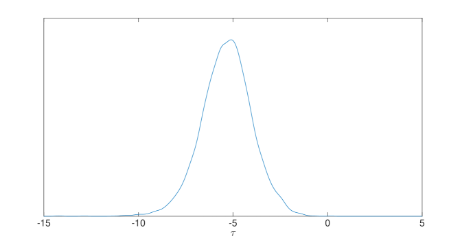
Figure 13: The posterior distribution of the average treatment effect (ATE) on subsequent annual earnings of a substantial lottery win for the lottery data set.

7 Conclusions

In this paper we have provided a coherent Bayesian calculus for rational nonparametric moment based estimators, allowing users to specify scientifically meaningful priors. At the core of our analysis is a prior density placed on the Hausdorff measure whose support is generated by the scientific parameters of interest and the nonparametric probabilities. We show how to transform this prior into a posterior density.

Much moment based analysis favoured in the literature delivers weakly identified parameters.  The use of very modest priors can dramatically improve estimation by downweighting vast regions of economically implausible parameter values.  Such weak priors play little role when the data is informative but provide a safety net when this is not the case.

To harness these gains, at the center of our paper are the marginal method and the joint method. The first is based on finding the density of the probabilities with respect to a Lebesgue measure. This allows for the use of conventional simulation methods such as MCMC, importance sampling and Hamiltonian Monte Carlo. It is convenient to use where the moment conditions can be solved analytically or numerically very fast.

Our joint method is somewhat harder to code but has the virtue of never having to solve the moment equations. This has some speed advantages but more fundamentally allows the rational analysis of moment condition models with many solutions. As a side product our method provides a novel way of generically simulating on a wide class of manifolds, which may be useful in other areas of science.

Appendix A Appendices

A.1 Proof of proposition 1

Since corresponding to every $\theta\in\Theta_{\theta}$ there is a unique $\beta$, there exist a one-to-one mapping between $\Theta_{\beta,\theta}$ and $\Theta_{\theta}$: $(\beta,\theta)=\left\{\beta(\theta),\theta)\right\}=F(\theta)$. Now let $A$ be a measurable set on $\Theta_{\beta,\theta}$, and assume $S_{\theta}(A)$ is its projection on $\Theta_{\theta}$. Therefore

$$\mathbb{P}(S_{\theta}(A))=\mathbb{P}(A)=\int_{A}p(\beta,\theta)dA=\int_{S_{\theta}(A)}\left\|v_{1}\wedge\cdots\wedge v_{J-1}\right\|p(\beta,\theta)dS$$

where $v_{j}=\frac{\partial F}{\partial\theta_{j}}$ (for $1\leq j\leq J-1$). Therefore $\left\|v_{1}\wedge\cdots\wedge v_{J-1}\right\|p(\beta,\theta)$ is the density of $\theta$ with respect to Lebesgue measure. Moreover,

$$\left\|v_{1}\wedge\cdots\wedge v_{J-1}\right\|=\left[Gram(v_{1},...,v_{J-1})\right]^{\frac{1}{2}}=\left|J_{\theta}^{\prime}J_{\theta}+I_{J-1}\right|^{\frac{1}{2}}=\left|J_{\theta}J_{\theta}^{\prime}+I_{p}\right|^{\frac{1}{2}}$$

where $Gram(\cdot)$ is the Gramian determinant and $J_{\theta}=\partial\beta/\partial\theta^{{}^{\prime}}$.

A.2 Proof of proposition 2

Let $p(\beta)$ be the density of $\beta$. Then, given $\beta$, the vector of probabilities $\theta$ lives on a $J-1-p$ dimensional hyperplane in $\mathbb{R}^{J-1}$ defined by $H\theta+g_{J}=0$. This system of equation can be solved for $p$ elements of the variables $\theta_{J-p:J-1}=-H_{2}^{-1}\left(H_{1}\theta_{1:J-p-1}-g_{J}\right)$, where $H_{1}=[h_{1}\ ...\ h_{J-p-1}]$ and $H_{2}=[h_{J-p}\ ...\ h_{J-1}]$. Therefore, $\partial\theta_{J-p:J-1}/\partial\theta_{1:J-p-1}=-H_{2}^{-1}H_{1}$ and so

$$p(\theta_{1:J-p-1}|\beta) = \left|H_{2}^{-1}H_{1}H_{1}^{\prime}H_{2}^{{}^{\prime}-1}+I_{p}\right|^{\frac{1}{2}}p(\theta|\beta),$$

$$p(\theta_{1:J-p-1},\beta) = \left|H_{2}^{-1}H_{1}H_{1}^{\prime}H_{2}^{{}^{\prime}-1}+I_{p}\right|^{\frac{1}{2}}p(\beta)p(\theta|\beta).$$

Therefore the density of $\theta$ is

$$p(\theta) = \left|\frac{\partial(\theta_{1:J-p-1},\beta)}{\partial(\theta)}\right|p(\theta_{1:J-p-1},\beta)=\left|\frac{\partial\beta}{\partial\theta_{J-p:J-1}}\right|p(\theta_{1:J-p-1},\beta)$$

$$= \left|\left[\mathbb{E}\left(\frac{\partial g}{\partial\beta^{\prime}}\right)\right]^{-1}H_{2}\right|p(\theta_{1:J-p-1},\beta)$$

$$= \left|\left[\mathbb{E}\left(\frac{\partial g}{\partial\beta^{\prime}}\right)\right]^{-1}H_{2}\right|\left|H_{2}^{-1}H_{1}H_{1}^{\prime}H_{2}^{{}^{\prime}-1}+I_{p}\right|^{\frac{1}{2}}p(\beta)p(\theta|\beta)$$

$$= \left|\left[\mathbb{E}\left(\frac{\partial g}{\partial\beta^{\prime}}\right)\right]^{-1}\right|\left|H_{1}H_{1}^{\prime}+H_{2}H_{2}^{\prime}\right|^{\frac{1}{2}}p(\beta)p(\theta|\beta)=\left|\left[\mathbb{E}\left(\frac{\partial g}{\partial\beta^{\prime}}\right)\right]^{-1}\right|\left|HH^{\prime}\right|^{\frac{1}{2}}p(\beta)p(\theta|\beta)$$

$$= \left|\left[\mathbb{E}\left(\frac{\partial g}{\partial\beta^{\prime}}\right)\right]^{-1}HH^{\prime}\left[\mathbb{E}\left(\frac{\partial g^{\prime}}{\partial\beta}\right)\right]^{-1}\right|^{\frac{1}{2}}p(\beta)p(\theta|\beta)=\left|\frac{\partial\beta}{\partial\theta^{{}^{\prime}}}\frac{\partial\beta^{\prime}}{\partial\theta}\right|^{\frac{1}{2}}p(\beta)p(\theta|\beta).$$

Therefore:

$$p(\beta,\theta)=\frac{\left|\frac{\partial\beta}{\partial\theta^{{}^{\prime}}}\frac{\partial\beta^{\prime}}{\partial\theta}\right|^{\frac{1}{2}}}{\left|\frac{\partial\beta}{\partial\theta^{{}^{\prime}}}\frac{\partial\beta^{\prime}}{\partial\theta}+I_{p}\right|^{\frac{1}{2}}}p(\beta)p(\theta|\beta).$$

A.3 Joint method proposal

In order to generate a proposal value for $\theta^{*}$, we can first draw $\pi^{\ast}$ from $\mathcal{N}(\theta,\Sigma_{Q})$, and let $\theta^{\ast}$ be the closest point to $\pi^{\ast}$ in the hyperplane $\mathcal{P}^{*}=\{\lambda\in\mathbb{R}^{J-1};H^{\ast}\lambda+g_{J}^{\ast}=0\}$, where we measure the distance between $\pi^{\ast}$ and $\theta^{\ast}$ with the squared Euclidean norm:

$$\theta^{\ast}=\underset{\theta}{\mathop{\mathrm{a}rgmin}}\ \frac{1}{2}\left\|\pi^{\ast}-\theta\right\|_{2}^{2}+\frac{1}{2}\left(\iota^{\prime}\pi^{\ast}-\iota^{\prime}\theta\right)^{2}.$$

The quadratic penalty is certainly inelegant (e.g. compared to the log-likelihood of the multinomial model, but see, for example, Owen (1991) and Antoine et al. (2007) who use it for their Euclidean empirical likelihood) as the resulting $\theta^{\ast}$ can have negative elements or may result in $\theta_{J}^{\ast}=1-\iota^{\prime}\theta^{\ast}\leq 0$. However, by using a quadratic penalty, $\theta^{\ast}$ becomes the solution to a quadratic optimization problem subject to $p$ equality constraints, and so has an analytic solution $\theta^{\ast}=a^{\ast}+B^{\ast}\pi^{\ast}$.

The Lagrangian of the optimization is,

$$E(\theta,\lambda)=\left\|\pi^{\ast}-\theta\right\|_{2}^{2}+\left(\iota^{\prime}\pi^{\ast}-\iota^{\prime}\theta\right)^{2}+\lambda^{\prime\ast}\theta+g_{J}^{\ast})$$

and the first order conditions are:

$$\frac{\partial E}{\partial\theta}=(I+\iota\iota^{\prime\ast}-\pi^{\ast})+H^{\ast^{\prime}}\lambda=0,\quad\frac{\partial E}{\partial\lambda}=H^{\ast}\theta^{\ast}+g_{J}^{\ast}=0.$$

Solving them for $\theta^{\ast}$ and $\lambda$ results in,

$$\theta^{\ast} = \pi^{\ast}-(I+\iota\iota^{\prime-1}H^{\ast^{\prime}}\left[H^{\ast}(I+\iota\iota^{\prime-1}H^{\ast^{\prime}}\right]^{-1}(H^{\ast}\pi^{\ast}+g_{J}^{\ast})$$

$$\lambda = \left[H^{\ast}(I+\iota\iota^{\prime-1}H^{\ast^{\prime}}\right]^{-1}(H^{\ast}\pi^{\ast}+g_{J}^{\ast}).$$

Therefore $\theta^{\ast}$ is an affine transformation of $\pi^{\ast}$: $\theta^{\ast}=a^{\ast}+B^{\ast}\pi^{\ast}$, where

$$a^{\ast} = -(I+\iota\iota^{\prime-1}H^{\ast^{\prime}}\left[H^{\ast}(I+\iota\iota^{\prime-1}H^{\ast^{\prime}}\right]^{-1}g_{J}^{\ast}$$

$$B^{\ast} = I-(I+\iota\iota^{\prime-1}H^{\ast^{\prime}}\left[H^{\ast}(I+\iota\iota^{\prime-1}H^{\ast^{\prime}}\right]^{-1}H^{\ast}.$$

This transformation from $\pi^{\ast}$ to $\theta^{\ast}$ is a many-to-one affine transformation. Consequently, $\theta^{\ast}|\beta^{\ast},\beta^{(t)},\theta^{(t)}$ is a singular normal distribution with mean $a^{\ast}+B^{\ast}\theta^{(t)}$ and variance matrix $B^{\ast}\Sigma_{Q}B^{\ast}$.

A singular normal distribution with mean $\mu$ and (singular) variance matrix $\Sigma$ has a density on the range of the covariance matrix (e.g. Khatri (1968)), given by

$$(2\pi)^{-\frac{1}{2}rank(\Sigma)}|\Sigma|_{{rank}(\Sigma)}^{-\frac{1}{2}}\exp\left\{-\frac{1}{2}\left(x-\mu\right)^{\prime}\Sigma^{+}\left(x-\mu\right)\right\},$$

where $|\Sigma|_{{rank}(\Sigma)}$ is the product of non-zero eigenvalues of $\Sigma$ and $\Sigma^{+}$ is its Moore-Penrose inverse.

In our algorithm, $\Sigma_{Q}$ and the parameters inside $q(\cdot|\beta^{(t)},\theta^{(t)})$ are the tuning parameters. We may either adapt them in the course of simulation, or they can be set to some fixed values obtained from an estimate of the posterior’s distribution. Here we document how we have carried this out for our simulation and empirical work. A simple to calculate candidate for the covariance of $\beta$’s proposal is $\Sigma_{\beta}=\left(\Sigma_{0_{\mathbf{\beta}}}^{-1}+\Sigma_{{BB}_{\mathbf{\beta}}}^{-1}\right)^{-1}$, where $\Sigma_{0_{\mathbf{\beta}}}^{-1}$ is the prior’s covariance and $\Sigma_{{BB}_{\mathbf{\beta}}}^{-1}$ is the covariance of the estimates of $\beta$ obtained by Bayesian bootstrapping of Chamberlain and Imbens (2003) (As an alternative we may use the asymptotic covariance of the least squares or GMM estimators). Moreover a suitable candidate for $\Sigma_{Q}$ is $diag(\hat{\theta}_{1}^{2},...,\hat{\theta}_{J-1}^{2})$ where:

$$\hat{\theta}=(\hat{\theta}_{1},...,\hat{\theta}_{J-1})=\underset{\theta}{\mathop{\mathrm{a}rgmax}}\sum_{j=1}^{J}n_{j}\ln\theta_{j}\ \ \ \text{subject to}\ \ \ \hat{H}\theta+\hat{g}_{J}=0,$$ (52)

in which $\hat{H}=\left(\hat{g}_{1},...,\hat{g}_{J-1}\right)-\hat{g}_{J}\iota^{\prime}$, $\hat{g}_{j}=g(\hat{\beta},s_{j})$ and $\hat{{\beta}}=\left({\Sigma}_{0_{{\beta}}}+{\Sigma}_{{BB}_{{\beta}}}\right)^{-1}\left({\Sigma}_{0_{{\beta}}}{\mu}_{{BB}_{{\beta}}}+{\Sigma}_{{BB}_{{\beta}}}{\mu}_{0_{{\beta}}}\right)$.

A.4 Large support

An apparent drawback of the joint method is that in each evaluation of the proposal’s density, the Moore-Penrose inverse of the $(J-1)\times(J-1)$ matrix $B^{\ast}\Sigma_{Q}B^{\ast\prime}$ should be computed. In general this costs $O(J^{3})$ computational operations.   This type of challenge is very common in Bayesian analysis and a standard approach to this problem is to make proposals to update a block of $K\ll J$ elements of $\theta$, with cost $O(K^{3})$.

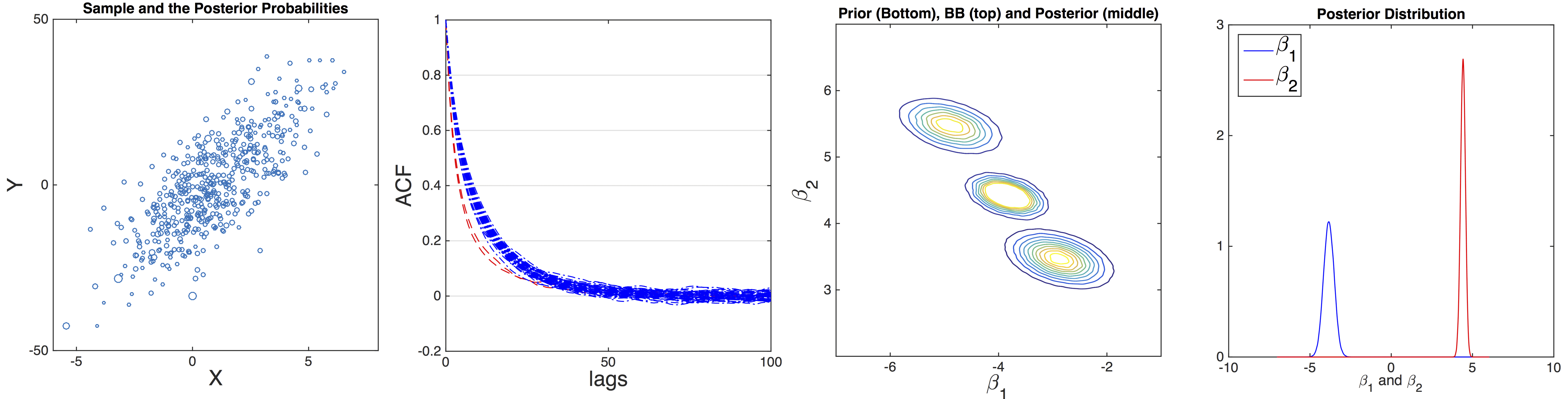
Figure 14: Inference in linear regression model with $J=500$ and an informative prior.

Let the $K\times 1$ vector $u$ be a randomly (without replacement) selected subset of the indices $\{1,...,J-1\}$ and the $(J-K-1)\times 1$ vector $v$ be its complement. Moreover let $\tilde{\theta}=(\theta_{u_{1}},...,\theta_{u_{K}})$ and $\bar{\theta}=(\theta_{v_{1}},...,\theta_{v_{J-K-1}})$. The proposal’s vector of probabilities, $\theta^{\ast}$, is equal to $\theta$ except for the $K$ elements with indices in $u$, $\tilde{\theta}^{\ast}=(\theta_{u_{1}}^{\ast},...,\theta_{u_{K}}^{\ast})$, that is obtained by solving:

$$\tilde{\theta}^{\ast}=\underset{\tilde{\theta}}{\mathop{\mathrm{a}rgmin}}\ \frac{1}{2}\|\tilde{\theta}-\tilde{\pi}^{\ast}\|+\frac{1}{2}\left(\iota^{\prime}\tilde{\theta}-\iota^{\prime}\tilde{\pi}^{\ast}\right)\ \ \ \text{subject to}\ \ \ \bar{H}^{\ast}\bar{\theta}^{(t)}+\tilde{H}^{\ast}\tilde{\theta}+g_{J}^{\ast}=0,$$ (53)

where $\tilde{H}^{\ast}=\left(g_{u_{1}}^{\ast},...,g_{u_{K}}^{\ast}\right)-g_{J}^{\ast}\iota^{\prime}$, $\bar{H}^{\ast}=\left(g_{v_{1}}^{\ast},...,g_{v_{J-K-1}}^{\ast}\right)-g_{J}^{\ast}\iota^{\prime}$, and $\tilde{\pi}^{\ast}$ is a random draw from $N(\tilde{\theta},\Sigma_{\tilde{\theta}})$. Again this is a quadratic optimization problem subject to a set of equality constraints with the following solution: $\tilde{\theta}^{\ast}=\tilde{a}^{\ast}+\tilde{B}^{\ast}\tilde{\pi}^{\ast}$, where

$$\tilde{a}^{\ast} = -(I+\iota\iota^{\prime-1}\tilde{H}^{\ast^{\prime}}\left[\tilde{H}^{\ast}(I+\iota\iota^{\prime-1}\tilde{H}^{\ast^{\prime}}\right]^{-1}\left(\bar{H}^{\ast}\bar{\theta}^{(t)}+g_{J}^{\ast}\right)$$

$$\tilde{B}^{\ast} = I-(I+\iota\iota^{\prime-1}\tilde{H}^{\ast^{\prime}}\left[\tilde{H}^{\ast}(I+\iota\iota^{\prime-1}\tilde{H}^{\ast^{\prime}}\right]^{-1}\tilde{H}^{\ast}.$$

A.5 Linear regression with an informative prior

Here we report the results for the linear regression model with sample size $J=500$, and an informative prior for $\beta$. We place a normal prior on $\beta$ with the mean equal to $\hat{\beta}_{\text{MLE}}+(5,-5)^{\prime}$ and the variance equal to the asymptotic variance of $\hat{\beta}_{\text{MLE}}$. Therefore the prior is as informative as the data, however centered at a significantly different point.

Figure 14’s top left panel shows a scatter plot of the sample. Each circle represents a data point and its radius is proportional to $\mathbb{E}(\theta_{j}|Z)$. In the top-right the ACF of the chains of $\beta$ and $50$ elements of $\theta$ have been presented (the red dashed lines and the blue dotted lines correspond to $\beta$ and $\theta$, respectively.) These show that the Markov chain is mixing sufficiently well. In the bottom-left panel the contour plot of the prior distribution (bottom), posterior distribution of $\beta$ using Bayesian bootstrapping, and the posterior distribution of $\beta$ considering the informative prior (middle) have been depicted. In the bottom-right panel the histogram of the samples from the posterior of $\beta$ can be seen.

A.6 Instrumental variables with partially observed support

Now we assume the support of $S=(X,Y,W)$ has other $J$ missing elements (not observed in the data), therefore $J^{\ast}=2J$. The density of our prior for the missing elements of the support is,

$$f_{S}(\tilde{s})=f_{S^{(1)}}(\tilde{s}^{(1)})f_{S^{(2)}}(\tilde{s}^{(2)})f_{S^{(3)}}(\tilde{s}^{(3)})$$ (54)

in which $f_{S^{(1)}}(\tilde{s}^{(1)})$ and $f_{S^{(3)}}(\tilde{s}^{(3)})$ are the density of a uniform distribution on $\{0,1,...,20\}$ and $\{0,1\}$, respectively, and $f_{S^{(2)}}(\tilde{s}^{(2)})$ is a normal density with mean $6$ and standard deviation $3$. Moreover we assume,

$$p(\beta,\theta^{\ast}|\tilde{S})\propto\frac{1}{\sqrt{J_{\theta^{\ast}}J_{\theta^{\ast}}^{\prime}+J_{\tilde{S}}J_{\tilde{S}}^{\prime}+I_{2}}}\eta(\beta)\eta(\theta^{\ast})1_{\Theta_{\beta,\theta^{\ast},\tilde{S}}}(\beta,\theta^{\ast},\tilde{S}),$$ (55)

where $\eta(\beta)=\varphi\left(\beta_{0};5,4\right)\varphi\left(\beta_{1};0,0.2\right)$ (similar to the previous case), and $\eta(\theta^{\ast})$ is the density a symmetric Dirichlet distribution with $\alpha=10^{-6}$. Hence the posterior distribution of $(\theta^{\ast},\tilde{S})$ is:

$$p(\theta^{\ast},\tilde{S}|Z)\propto\eta(\beta)\left(\prod_{j=1}^{\tilde{J}}f_{S}(\tilde{s}_{j})\right)\left(\prod_{j=1}^{J^{\ast}}\theta_{j}^{\ast^{n_{j}+\alpha-1}}\right).$$ (56)

To sample from this distribution we can reweight random draws from the following proposal,

$$g(\theta^{\ast},\tilde{S}|Z)\propto\left(\prod_{j=1}^{\tilde{J}}f_{S}(\tilde{s}_{j})\right)\left(\prod_{j=1}^{J^{\ast}}\theta_{j}^{\ast^{n_{j}+\alpha-1}}\right),$$ (57)

with he weights proportional to $\eta(\beta)$. Now we set $J=10$, and for $1000$ times we draw a random sample from our dataset. Then we compare the posterior distribution of the parameters under two assumptions. In the first model we assume the support of $S$ is fully observed in the data (similar to the previous section of this example), while in the second model we assume the data has $\tilde{J}=10$ more elements that are not observed in our sample. Since the prior of the probabilities and $\beta$ is barely informative the posterior distributions of $\beta$ are almost indistinguishable under these two assumptions.

A.7 Not the just identified case

A.7.1 Abstract expression of the problem

Collect all the parameters in the model and constraints as

$$\psi=(\theta_{1},...,\theta_{J-1},\beta_{1},...,\beta_{p})^{\prime},\quad g(\psi)=0_{r}.$$

Then resulting constrained support is $\psi\in\Theta_{\psi}$. Write $\lambda=\psi_{\mathcal{I}}$, $\phi=\psi_{\mathcal{I}^{c}}$, where $\mathcal{I}$ selects distinct indexes of $\psi$ and $\mathcal{I}^{c}$ is the complement, so $\mathcal{I\cup I}^{c}=\left\{1,2,...,p+J-1\right\}$.  Throughout we take $\dim(\phi)=r$ and consequently $\dim(\lambda)=J-m$, where $m=r-p+1$.

Given the freedom to build $\mathcal{I}$ we make the following assumption.

Assumption A.  Under $g(\psi)=0$ knowledge of $\lambda$ reveals $\phi$, so there exists a unique $\phi=t(\lambda)$.

A.7.2 Marginal method

Under Assumption A, the area formula implies that $p(\lambda)=p(\psi)\sqrt{\left|I_{r}+J_{\phi\lambda}J_{\phi\lambda}^{\prime}\right|}$, $J_{\phi\lambda}=\partial\phi/\partial\lambda^{\prime}$, where $p(\psi)$ is a density with respect to the $(J-1+p-r)$-dimensional Hausdorff measure on $\Theta_{\psi}$, while $p(\lambda)$ is a density with respect to the $J-m$-dimensional Lebesgue measure.

A.7.3 Underidentification

Definition 1

If $r<p$ (so $m\leq 0$) then the system is called underidentified.

We split $\beta=\left(\beta_{1},...,\beta_{p}\right)^{\prime}$ as $\beta_{[1]}=\beta_{\mathcal{J}}$, $\beta_{[2]}=\beta_{\mathcal{J}^{c}}$, where $\mathcal{J\cup J}^{c}=\left\{1,2,...,p\right\}$, $\dim(\mathcal{J})=p-r$ and $\dim(\mathcal{J}^{c})=r$, and build $\lambda=(\theta_{1},...,\theta_{J-1},\beta_{[1]}^{\prime})^{\prime}$, $\phi=\beta_{[2]}$. Hence $\lambda$ augments $\theta$ with $p-r$ elements from $\beta$. Assumption A holds if $\mathcal{J}$ can be found such that $\beta_{[2]}=t(\theta_{1},...,\theta_{J-1},\beta_{[1]})$.

Example 11

Consider instrumental variables problem $g(s,\beta)=s^{(3)}\left\{s^{(1)}-\beta^{\prime}s^{(2)}\right\}$, $\dim(s^{(2)})=p$, $\dim(s^{(3)})=r$. If $p>r$ then split $\beta=\left(\beta_{[1]}^{\prime},\beta_{[2]}^{\prime}\right)^{\prime}$, where $\dim(\beta_{[1]})=r-p$ and $\dim(\beta_{[2]})=r$. Write $s_{j}=\left(s_{j,[1]}^{\prime},s_{j,[2]}^{\prime}\right)^{\prime}$, then

$$\sum_{j=1}^{J}\theta_{j}s_{j}^{(3)}\left\{\left(s_{j}^{(1)}-\beta_{[1]}^{\prime}s_{j,[1]}^{(2)}\right)-\beta_{[2]}^{\prime}s_{j,[2]}^{(2)}\right\}=0_{r}.$$

Knowledge of $\beta_{[1]}$ puts us back to the just identified, so Assumption A holds under weak assumptions and so $p(\theta,\beta_{[2]})$ can be computed using the area formula.

A.7.4 Overidentification  

Definition 2

If $r>p$ so $m\geq 1$ (e.g. $r=2$,$p=1$, $m=2$) then the system is called overidentified.

We split $\theta=\left(\theta_{1},...,\theta_{J-1}\right)^{\prime}$ as $\theta_{[1]}=\theta_{\mathcal{J}}$, $\theta_{[2]}=\theta_{\mathcal{J}^{c}},$where $\mathcal{J\cup J}^{c}=\left\{1,2,...,J-1\right\}$, $\dim(\mathcal{J})=J-m$ and $\dim(\mathcal{J}^{c})=m-1$, and build $\lambda=\theta_{[1]}^{\prime}$, $\phi=\left(\theta_{[2]}^{\prime},\beta^{\prime}\right)^{\prime}$. Hence $\lambda$ is a subset of $\theta$ with $J-m$ elements, while $\phi$ contains all the other probabilities and the entire $\beta$. Then Assumption A holds if we can find a $\mathcal{J}$ such that $\left(\theta_{[2]}^{\prime},\beta^{\prime}\right)^{\prime}=t(\theta_{[1]}^{\prime})$.

Example 12

Again consider $g(s,\beta)=s^{(3)}\left\{s^{(1)}-\beta^{\prime}s^{(2)}\right\}$, $\dim(s^{(2)})=p$, $\dim(s^{(3)})=r$. If $p<r$ then split $\theta=\left(\theta_{[1]}^{\prime},\theta_{[2]}^{\prime}\right)^{\prime}$, where $\dim(\theta_{[2]}^{\prime},\beta^{\prime})=r$, so there are $r$ moment conditions and $r$ unknowns. Given $\theta_{[1]}$, we can then solve for the extended set of parameters $\left(\theta_{[2]}^{\prime},\beta^{\prime}\right)$, where

$$\sum_{j=1}^{\dim(\theta_{[1]})}\theta_{j}s_{j}^{(3)}\left\{s_{j}^{(1)}-\beta^{\prime}s_{j}^{(2)}\right\}+\sum_{j=\dim(\theta_{[1]})+1}^{J}\theta_{j}s_{j}^{(3)}\left\{s_{j}^{(1)}-\beta^{\prime}s_{j}^{(2)}\right\}=0_{r}.$$

This is typically exactly identified, but non-linear due to the $\theta_{j}\beta$ terms for $j=\dim(\theta_{[1]})+1,...,J$.

References

• Angrist and Krueger (1991) Angrist, J. D. and A. B. Krueger (1991). Does compulsory school attendance affect schooling and earnings? The Quarterly Journal of Economics 106, 979–1014.
• Antoine et al. (2007) Antoine, A., H. Bonnal, and E. Renault (2007). On the efficient use of the informational content of estimating equations: implied probabilities and Euclidean empirical likelihood. Journal of Econometrics 138, 461–487.
• Ariyabuddhiphongs (2011) Ariyabuddhiphongs, V. (2011). Lottery gambling: A review. Journal of Gambling Studies 27, 15–33.
• Bound et al. (2001) Bound, J., C. Brown, and N. Mathiowetz (2001). Measurement error in survey data. In J. J. Heckman and E. Leamer (Eds.), Handbook of Econometrics, Volume 5, pp.  3705–3843. North Holland.
• Bound et al. (1995) Bound, J., D. A. Jaeger, and R. M. Baker (1995). Problems with instrumental variables estimation when the correlation between the instruments and the endogenous explanatory variable is weak. Journal of the American Statistical Association 90, 443–450.
• Britton et al. (2015) Britton, J., N. Shephard, and A. Vignoles (2015). Comparing sample survey measures of English earnings of graduates with administrative data. Unpublished paper: Department of Economics, Harvard University.
• Brubaker et al. (2012) Brubaker, M., M. Salzmann, and R. Urtasun (2012). A family of MCMC methods on implicitly defined manifolds. In: JMLR Workshop and Conference Proceedings 20, 161–172.
• Byrne and Girolami (2013) Byrne, S. and M. Girolami (2013). Geodesic Monte Carlo on embedded manifolds. Scandinavian Journal of Statistics 40, 825–845.
• Chamberlain (1987) Chamberlain, G. (1987). Asymptotic efficiency in estimation with conditional moment restrictions. Journal of Econometrics 34, 305–334.