Local Likelihood Estimation for Covariance Functions with Spatially-Varying Parameters: The convoSPAT Package for R

Mark D. Risser, Catherine A. Calder Local Likelihood Estimation for Covariance Functions with Spatially-Varying Parameters: The convoSPAT Package for R convoSPAT: Local Likelihood Estimation for Spatially-Varying Covariance Functions In spite of the interest in and appeal of convolution-based approaches for nonstationary spatial modeling, off-the-shelf software for model fitting does not as of yet exist. Convolution-based models are highly flexible yet notoriously difficult to fit, even with relatively small data sets. The general lack of pre-packaged options for model fitting makes it difficult to compare new methodology in nonstationary modeling with other existing methods, and as a result most new models are simply compared to stationary models. Using a convolution-based approach, we present a new nonstationary covariance function for spatial Gaussian process models that allows for efficient computing in two ways: first, by representing the spatially-varying parameters via a discrete mixture or “mixture component” model, and second, by estimating the mixture component parameters through a local likelihood approach. In order to make computations for a convolution-based nonstationary spatial model readily available, this paper also presents and describes the convoSPAT package for R. The nonstationary model is fit to both a synthetic data set and a real data application involving annual precipitation to demonstrate the capabilities of the package. spatial statistics, nonstationary modeling, local likelihood estimation, precipitation, R spatial statistics, nonstationary modeling, local likelihood estimation, precipitation, R Catherine A. Calder
Department of Statistics
The Ohio State University
1958 Neil Avenue
Columbus, OH, USA 43210
E-mail:

1 Introduction

The Gaussian process is an extremely popular modeling approach in modern-day spatial and environmental statistics, due largely to the fact that the model is completely characterized by first- and second-order properties, and the second-order properties are straightforward to specify through widely used classes of valid covariance functions. A broad literature on covariance function modeling exists, but traditional approaches are mostly based on assumptions of isotropy or stationarity, in which the covariance between the spatial process at two locations is a function of only the separation distance or separation vector, respectively. This modeling assumption is made mostly for convenience, and is rarely a realistic assumption in practice. As a result, a wide variety of nonstationary covariance function models for Gaussian process models have been developed (e.g., sampGutt; Higdon98; damian2001; fuentes2001; schmidt03; PacScher; calder08; schmidt11; reich2011; and ViannaNeto), in which the spatial dependence structure is allowed to vary over the spatial region of interest. However, while these nonstationary approaches more appropriately model the covariance in the spatial process, most are also highly complex and require intricate model-fitting algorithms, making it very difficult to replicate their results in a general setting. Therefore, when new nonstationary methods are developed, their performance is usually compared to stationary models, for which robust software is available. While software exists for several of these nonstationary approaches (see below), there are currently no pre-packaged options for fitting convolution-based nonstationary models.

To address this need, we present a simplified version of the nonstationary spatial Gaussian process model introduced by PacScher in which the locally-varying geometric anisotropies are modeled using a “mixture component” approach, similar to the discrete mixture kernel convolution approach in Higdon98 but allowing the underlying correlation structure to be specified by the modeler. The model is extended to allow other properties to vary over space as well, such as the process variance, nugget effect, and smoothness. An additional degree of efficiency is gained by using local likelihood techniques to estimate the spatially-varying features of the spatial process; then, the locally estimated features are smoothed over space, similar in nature to the approach of fuentes02.

This paper also presents and describes the convoSPAT package for R for conducting a full analysis of point-referenced spatial data using a convolution-based nonstationary spatial Gaussian process model. The primary contribution of the package is to provide accessible model-fitting tools for spatial data of this type, as software for convolution-based nonstationary modeling does not currently exist. Furthermore, the methods used by the package are computationally efficient even when the size of the data is relatively large (on the order of $n=1000$). The package is able to handle both a single realization of the spatial process observed at a finite set of locations, as well as independent and identically distributed replicates of the spatial process observed at a common set of locations. Finally, the paper demonstrates how the package can be used, and provides analyses of both simulated and real data sets.

As noted, there are several other (albeit non convolution-based) methods for nonstationary spatial modeling that do offer software, namely the basis function approach in the fields package (R_fields) and the Gaussian Markov random field approach in the INLA package (Lindgren2011; spde13; Fuglstad2015; Lindgren2015), both available for R. However, as these methods arise from significantly different modeling approaches, the convoSPAT package represents a novel contribution to the set of available software for nonstationary spatial modeling. Comparison across software for these various packages is beyond the scope of this paper and will be reserved for future work.

The paper is organized as follows. Section 2 introduces a convolution-based approach for nonstationary spatial statistical modeling, and Section 3 describes a full model for observed data and the mixture component parameterization. Section 4 outlines a computationally efficient approach to inference for the model introduced in Section 3; Sections 5, 6, and LABEL:USprecip outline usage of the convoSPAT package and present two applications. Section LABEL:discussion concludes the paper.

2 A convolution-based nonstationary covariance function

Process convolutions or moving average models are popular constructive methods for specifying a nonstationary process model. In general, a spatial stochastic process $Y(\cdot)$ on $G\subset\mathcal{R}^{d}$ can be defined by the kernel convolution

$$Y({\bf s})=\int_{\mathcal{R}^{d}}K_{\bf s}({\bf u})dW({\bf u}),$$ (1)

where $W(\cdot)$ is a $d$-dimensional stochastic process and $K_{\bf s}(\cdot)$ is a (possibly parametric) spatially-varying kernel function centered at ${\bf s}\in G$. higdon2 summarizes the extremely flexible class of spatial process models defined by Equation 1: see, for example, Barry1996, VerHoef2004, Wolpert1999, Higdon98, VerHoef2004, and Barry_VerHoef1998.

The kernel convolution Equation 1 defines a mean-zero nonstationary spatial Gaussian process (GP) if $W(\cdot)$ is chosen to be $d$-dimensional Brownian motion. A benefit of using Equation 1 is that in this case the kernel functions completely specify the second-order properties of the GP through the covariance function

$$\operatorname{Cov}(Y({\bf s}),Y({\bf s^{\prime})})=E\big{[}Y({\bf s})Y({\bf s^{\prime}})\big{]}=\int_{G}K_{\bf s}({\bf u})K_{\bf s^{\prime}}({\bf u})d{\bf u},$$ (2)

where ${\bf s,s^{\prime}}\in G$. The popularity of this approach is due largely to the fact that it is much easier to specify kernel functions than a covariance function directly, since the kernel functions only require $\int_{\mathcal{R}^{d}}K_{\bf s}({\bf u})d{\bf u}<\infty$ and $\int_{\mathcal{R}^{d}}K^{2}_{\bf s}({\bf u})d{\bf u}<\infty,$ while a covariance function must be even and nonnegative definite (BochnerBook; AdlerBook). A famous result (thiebaux76; thiebaux_pedder) uses a parametric class of Gaussian kernel functions in Equation 2 to give a closed-form covariance function; this result was later extended (paciorek2003; PacScher; stein2005) to show that

$$C^{NS}({\bf s},{\bf s^{\prime}};{\boldsymbol{\theta}})=\sigma({\bf s})\sigma({\bf s^{\prime}})\frac{\left|{\bf\Sigma(s)}\right|^{1/4}\left|{\bf\Sigma(s^{\prime})}\right|^{1/4}}{\left|\frac{{\bf\Sigma(s)+\Sigma(s^{\prime})}}{2}\right|^{1/2}}g\left(\sqrt{Q({\bf s,s^{\prime}})}\right),$$ (3)

is a valid, nonstationary, parametric covariance function on $\mathcal{R}^{d},d\geq 1$, when $g(\cdot)$ is chosen to be a valid correlation function on $\mathcal{R}^{d},d\geq 1$. Note that Equation 3 no longer requires kernel functions to be specified. In Equation 3, $\boldsymbol{\theta}$ is a generic parameter vector, $\sigma(\cdot)$ represents a spatially-varying standard deviation, ${\bf\Sigma}(\cdot)$ is a $d\times d$ matrix that represents the spatially-varying local anisotropy (controlling both the range and direction of dependence), and

$$Q({\bf s,s^{\prime}})={\bf(s-s^{\prime})}^{\top}\left(\frac{{\bf\Sigma(s)+\Sigma(s^{\prime})}}{2}\right)^{-1}{\bf(s-s^{\prime})}$$ (4)

is a Mahalanobis distance. Furthermore, choosing $g(\cdot)$ to be the Matérn correlation function also allows for the introduction of $\kappa(\cdot)$, a spatially-varying smoothness parameter (stein2005; in this case, the Matérn correlation function in Equation 3 has smoothness $[\kappa({\bf s})+\kappa({\bf s}^{\prime})]/2$). While using Equation 3 no longer requires the notion of kernel convolution, we refer to ${\bf\Sigma}(\cdot)$ as the kernel matrix, since it was originally defined as the covariance matrix of a Gaussian kernel function (thiebaux76; thiebaux_pedder). The covariance function in Equation 3 is extremely flexible, and has been used in various forms throughout the literature, e.g., PacScher, Anderes_Stein, kleiber2012, Katzfuss2013, and Risser15.

3 A nonstationary spatial Gaussian process model

The covariance function in Equation 3 can be used to define a nonstationary spatial Gaussian process model using the following framework. Let $\{Z({\bf s}),{\bf s}\in G\}$ be a spatial field defined on $G\subset\mathcal{R}^{d}$, where

$$Z({\bf s})={\bf x}({\bf s})^{\top}\boldsymbol{\beta}+Y({\bf s})+\epsilon({\bf s}).$$ (5)

In Equation 5, the mean of the spatial field is $E[Z({\bf s})]={\bf x}({\bf s})^{\top}\boldsymbol{\beta}$, where ${\bf x}({\bf s})$ is a $p$-vector of covariates for location ${\bf s}$ and $\boldsymbol{\beta}\in\mathcal{R}^{p}$ are unknown regression coefficients. $Y(\cdot)$ represents a spatially-dependent, mean-zero Gaussian process with covariance function $C^{NS}$ from Equation 3, while $\epsilon(\cdot)$ represents measurement error and, given $\tau^{2}(\cdot)$, is conditionally independent $\mathcal{N}(0,\tau^{2}({\bf s}))$. (Note: $\mathcal{N}(a,b)$ denotes the univariate Gaussian distribution with mean $a$ and variance $b$.) The spatially-referenced random components, $\epsilon(\cdot)$ and $Y(\cdot)$, are assumed to be mutually independent. Finally, define ${\boldsymbol{\theta}}$ to be a vector of all the variance-covariance parameters from the Gaussian process $Y(\cdot)$ and error process $\epsilon(\cdot)$.

Now, suppose we have observations which are a partial realization of $Z(\cdot)$, taken at a fixed, finite set of $n$ spatial locations $\{{\bf s}_{i}\}_{i=1}^{n}\in G$, giving the random (observed) vector ${\bf Z}=\left(Z({\bf s}_{1}),...,Z({\bf s}_{n})\right)$. The model in Equation 5 implies that ${\bf Z}$ has a multivariate Gaussian distribution, conditional on the unobserved latent process ${\bf Y}=\left(Y({\bf s}_{1}),...,Y({\bf s}_{n})\right)$ and all other model parameters:

$${\bf Z}|{\bf Y},{\boldsymbol{\beta}},{\boldsymbol{\theta}}\sim\mathcal{N}_{n}\big{(}{\bf X}\boldsymbol{\beta}+{\bf Y},{\bf D}({\boldsymbol{\theta}})\big{)},$$ (6)

where the $i$th row of ${\bf X}$ is ${\bf x}({\bf s}_{i})$ and ${\bf D}({\boldsymbol{\theta}})$ is a diagonal matrix with $(i,i)$ element $\tau^{2}({\bf s}_{i})$. (Note: $\mathcal{N}_{q}({\bf a},{\bf B})$ denotes the $q$-variate Gaussian distribution with mean vector ${\bf a}$ and covariance ${\bf B}$.) Integrating out the process ${\bf Y}$ from Equation 6, we can obtain the marginal likelihood of the observed data ${\bf Z}$ given all parameters, which is

$${\bf Z}|{\boldsymbol{\beta}},{\boldsymbol{\theta}}\sim\mathcal{N}_{n}\big{(}{\bf X}\boldsymbol{\beta},{\bf D({\boldsymbol{\theta}})+\Omega({\boldsymbol{\theta}})}\big{)},$$ (7)

where ${\bf\Omega({\boldsymbol{\theta}})}$ has elements $\Omega_{ij}({\boldsymbol{\theta}})=C^{NS}({\bf s}_{i},{\bf s}_{j};\boldsymbol{\theta})$. For a particular application, the practitioner can specify the underlying correlation structure (through $g(\cdot)$) as well as determine which of $\{{\bf\Sigma}(\cdot),\sigma(\cdot),\tau^{2}(\cdot)\}$ (or $\kappa(\cdot)$, if the Matérn is used) should be fixed or allowed to vary spatially. However, some care should be taken in choosing which quantities should be spatially-varying: for example, Anderes_Stein note that allowing both ${\bf\Sigma}(\cdot)$ and $\kappa(\cdot)$ to vary over space leads to issues with identifiability.

3.1 Discrete mixture representation

One way to reduce the computational demands of fitting a Gaussian process-based spatial model with parametric covariance function given by Equation 3 is by characterizing the nonstationary behavior of a spatial process through the discretized basis kernel approach of Higdon98. Higdon98 estimated the Gaussian kernel function for a generic location to be a weighted average of “basis” kernel functions, estimated locally over the spatial region of interest. However, since the use of Gaussian kernel functions results in undesirable smoothness properties (see, e.g., PacScher), we instead use a related “mixture component” approach, in which the parametric quantities for an arbitrary spatial location are defined as a mixture of spatially-varying parameter values associated with a fixed set of component locations. Specifically, in this new approach, we define mixture component locations $\{{\bf b}_{k}:k=1,\dots,K\}$ with corresponding parameters $\{({\bf\Sigma}_{k},\sigma^{2}_{k},\tau^{2}_{k},\kappa_{k}):k=1,\dots,K\}$ (which are the kernel matrix, variance, nugget variance, and smoothness, respectively). Then, for $\phi\in\{{\bf\Sigma},\sigma^{2},\tau^{2},\kappa\}$, the parameter set for an arbitrary location ${\bf s}\in G$ is calculated as

$$\phi({\bf s})=\sum_{k=1}^{K}w_{k}({\bf s})\phi_{k},$$ (8)

where

$$w_{k}({\bf s})\propto\exp\left\{-\frac{||{\bf s-b}_{k}||^{2}}{2\lambda_{w}}\right\}$$ (9)

such that $\sum_{k=1}^{K}w_{k}({\bf s})=1$. For example, the kernel matrix for ${\bf s}\in G$ is ${\bf\Sigma(s)}=\sum_{k=1}^{K}w_{k}({\bf s}){\bf\Sigma}_{k}$. In Equation 9, $\lambda_{w}$ acts as a tuning parameter, ensuring that the rate of decay in the weighting function is appropriate for both the data set and scale of the spatial domain. Using this approach, the number of parameters is now linear in $K$, the number of mixture component locations, instead of $n$, the sample size. Furthermore, this specification still enables the modeler to choose which parameters should be spatially-varying: the kernel matrices, the process variance, the nugget variance, and the smoothness.

3.2 Prediction

Define ${\bf Z}^{*}=\left(Z({\bf s}^{*}_{1}),...,Z({\bf s}^{*}_{m})\right)$ to be a vector of the process values at all prediction locations of interest. The Gaussian process model in Equation 5 implies that

$$\left[\begin{array}[]{c}{\bf Z}\\ {\bf Z^{*}}\end{array}\Bigg{|}\hskip 4.30554pt\boldsymbol{\beta,\theta}\hskip 4.30554pt\right]\sim\mathcal{N}_{n+m}\left(\left[\begin{array}[]{c}{\bf X}\boldsymbol{\beta}\\ {\bf X}^{*}\boldsymbol{\beta}\end{array}\right],\left[\begin{array}[]{cc}{\bf D}({\boldsymbol{\theta}})+{\bf\Omega}({\boldsymbol{\theta}})&{\bf\Omega_{ZZ^{*}}({\boldsymbol{\theta}})}\\ {\bf\Omega_{Z^{*}Z}({\boldsymbol{\theta}})}&{\bf D}^{*}({\boldsymbol{\theta}})+{\bf\Omega}^{*}({\boldsymbol{\theta}})\end{array}\right]\right),$$

where $\operatorname{Cov}({\bf Z}^{*})={\bf D}^{*}({\boldsymbol{\theta}})+{\bf\Omega}^{*}({\boldsymbol{\theta}})$ and $\operatorname{Cov}({\bf Z,Z}^{*})={\bf\Omega_{ZZ^{*}}({\boldsymbol{\theta}})}$. By the properties of the multivariate Gaussian distribution,

$${\bf Z^{*}|Z=z},\boldsymbol{\beta,\theta}\sim\mathcal{N}_{m}(\boldsymbol{\mu}_{\bf Z^{*}|z},{\bf\Sigma}_{\bf Z^{*}|z}),$$ (10)

where

$$\boldsymbol{\mu}_{\bf Z^{*}|z}={\bf X}^{*}\boldsymbol{\beta}+{\bf\Omega_{Z^{*}Z}}({\boldsymbol{\theta}})[{\bf D}({\boldsymbol{\theta}})+{\bf\Omega}({\boldsymbol{\theta}})]^{-1}({\bf z}-{\bf X}\boldsymbol{\beta}),$$ (11)

and

$${\bf\Sigma}_{\bf Z^{*}|z}=[{\bf D}^{*}({\boldsymbol{\theta}})+{\bf\Omega}^{*}({\boldsymbol{\theta}})]-{\bf\Omega_{Z^{*}Z}}({\boldsymbol{\theta}})[{\bf D}({\boldsymbol{\theta}})+{\bf\Omega}({\boldsymbol{\theta}})]^{-1}{\bf\Omega_{ZZ^{*}}({\boldsymbol{\theta}})}.$$ (12)

Using plug-in estimates $\widehat{\boldsymbol{\beta}}$ and $\widehat{\boldsymbol{\theta}}$ (see Section 4), the predictor for ${\bf Z}^{*}$ is then $\widehat{\boldsymbol{\mu}}_{\bf Z^{*}|z}$ with corresponding prediction errors as the square root of the diagonal elements of $\widehat{\bf\Sigma}_{\bf Z^{*}|z}$.

3.2.1 Out-of-sample evaluation criteria

Three cross-validation evaluation criteria can be used to assess the fit of the nonstationary spatial model given in Equation 5. First, the mean squared prediction error

$$MSPE=\frac{1}{m}\sum_{j=1}^{m}(z^{*}_{j}-\widehat{z}^{*}_{j})^{2},$$ (13)

where $z^{*}_{j}$ is the $j$th held-out observed (or “validation”) value and $\widehat{z}^{*}_{j}$ is the corresponding predictor (from Equation 11). The MSPE is a point-wise measure of model fit, and smaller MSPE indicates better predictions.

Second, to assess the prediction error relative to the standard error of each prediction, we use the so-called prediction mean squared deviation ratio

$$pMSDR=\frac{1}{m}\sum_{j=1}^{m}\frac{(z^{*}_{j}-\widehat{z}^{*}_{j})^{2}}{\widehat{\sigma}_{j}},$$ (14)

where $z^{*}_{j}$ and $\widehat{z}^{*}_{j}$ are defined as above and $\widehat{\sigma}_{j}$ is the prediction error corresponding to $\widehat{z}^{*}_{j}$ (from Equation 12).

Finally, the continuous rank probability score will be used (a proper scoring rule; see PropScoring). For the $j$th prediction, this is defined as

$$CRPS_{j}\equiv CRPS(F_{j},z^{*}_{j})=-\int_{-\infty}^{\infty}\big{(}F_{j}(x)-{1}\{x\geq z^{*}_{j}\}\big{)}^{2}dx,$$ (15)

where $F_{j}(\cdot)$ is the cumulative distribution function (CDF) for the predictive distribution of $z^{*}_{j}$ given the training data and ${1}\{\cdot\}$ is the indicator function. In this case, given that the predictive CDF is Gaussian (conditional on parameters; see Equation 10), a computational shortcut can be used for calculating Equation 15: when $F$ is Gaussian with mean $\mu$ and variance $\sigma^{2}$,

$$CRPS\big{(}F,z^{*}_{j}\big{)}=\sigma\Bigg{[}\frac{1}{\sqrt{\pi}}-2\cdot\phi\left(\frac{z^{*}_{j}-\mu}{\sigma}\right)-\frac{z^{*}_{j}-\mu}{\sigma}\left(2\cdot\Phi\left(\frac{z^{*}_{j}-\mu}{\sigma}\right)-1\right)\Bigg{]},$$

where $\phi$ and $\Phi$ denote the probability density and cumulative distribution functions, respectively, of a standard Gaussian random variable. The reported metric will be the average over all validation locations, $\widehat{CRPS}=m^{-1}\sum_{j=1}^{m}\widehat{CRPS}_{j}.$ CRPS measures the fit of the predictive density; larger CRPS (i.e., smaller negative values) indicates better model fit.

4 Computationally efficient inference

As discussed in Section 1, fast and efficient inference for a nonstationary process convolution model has yet to be made readily available for general use. In spite of its popularity, the use of Equation 3 always requires some kind of constraints and has suffered from a lack of widespread use due to the complexity of the requisite model fitting and limited pre-packaged options. Focusing on the spatially-varying local anisotropy matrices ${\bf\Sigma}(\cdot)$, the covariance function in Equation 3 requires a kernel matrix at every observation and prediction location of interest. PacScher accomplish this by modeling ${\bf\Sigma}(\cdot)$ as itself a (stationary) stochastic process, assigning Gaussian process priors to the elements of the spectral decomposition of ${\bf\Sigma}(\cdot)$; alternatively, Katzfuss2013 uses a basis function representation of ${\bf\Sigma}(\cdot)$. Both of these models are highly parameterized and require intricate Markov chain Monte Carlo methods for model fitting.

The approach we propose provides efficiency in two ways: first, from the model itself, which uses a discrete mixture representation (see Section 3.1), and second, by fitting the mixture components of the model locally, using the idea of local likelihood estimation (TibshiraniHastie).

4.1 Local likelihood estimation

Using the discrete mixture representation of Equation 8, a “full likelihood” approach to parameter estimation could be taken, in either a Bayesian or maximum likelihood framework, although the optimization in a maximum likelihood approach could become intractable for either moderately large $K$ or large $n$. However, since the primary goal of this new methodology is computational speed, a further degree of efficiency can be gained by using local likelihood estimation (LLE; TibshiraniHastie).

Before discussing the local likelihood approach, we outline a restricted maximum likelihood (REML; see patterson_thompson1971, patterson_thompson1974, and kitanidis1983) approach for separating estimation of the mean parameters $\boldsymbol{\beta}$ from the covariance parameters $\boldsymbol{\theta}$. The full log-likelihood for $\boldsymbol{\beta}$ and $\boldsymbol{\theta}$ in Equation 5 is

$$\mathcal{L}^{F}(\boldsymbol{\beta,\theta};{\bf Z})=-\frac{1}{2}\log|{\bf\Omega}+{\bf D}|-\frac{1}{2}({\bf Z-X\boldsymbol{\beta}})^{\top}({\bf\Omega}+{\bf D})^{-1}({\bf Z-X\boldsymbol{\beta}}),$$ (16)

where we have abbreviated ${\bf D}\equiv{\bf D}({\boldsymbol{\theta}})$ and ${\bf\Omega}\equiv{\bf\Omega}({\boldsymbol{\theta}})$; a standard maximum likelihood approach would set out to maximize $\mathcal{L}^{F}(\boldsymbol{\beta,\theta};{\bf Z})$ directly. REML, on the other hand, uses a (log) likelihood based on $n-p$ linearly independent linear combinations of the data that have an expected value of zero for all possible $\boldsymbol{\beta}$ and $\boldsymbol{\theta}$. Regardless of which set of linearly independent combinations is chosen, the “restricted” log-likelihood, which depends only on $\boldsymbol{\theta}$, is

$$\mathcal{L}^{R}(\boldsymbol{\theta};{\bf Z})=-\frac{1}{2}\log|{\bf\Omega}+{\bf D}|-\frac{1}{2}\log|{\bf X}^{\top}({\bf\Omega}+{\bf D})^{-1}{\bf X}|-\frac{1}{2}{\bf Z}^{\top}{\bf P}{\bf Z},$$ (17)

where

$${\bf P}=({\bf\Omega}+{\bf D})^{-1}-({\bf\Omega}+{\bf D})^{-1}{\bf X}\big{(}{\bf X}^{\top}({\bf\Omega}+{\bf D})^{-1}{\bf X}\big{)}^{-1}{\bf X}^{\top}({\bf\Omega}+{\bf D})^{-1}.$$ (18)

The REML estimate of $\boldsymbol{\theta}$ is obtained by maximizing $\mathcal{L}^{R}(\boldsymbol{\theta};{\bf Z})$, and the estimate of $\boldsymbol{\beta}$ is the generalized least squares estimate

$$\widehat{\boldsymbol{\beta}}=\big{(}{\bf X}^{\top}(\widehat{{\bf\Omega}}+\widehat{{\bf D}})^{-1}{\bf X}\big{)}^{-1}{\bf X}^{\top}(\widehat{{\bf\Omega}}+\widehat{{\bf D}})^{-1}{\bf Z},$$ (19)

which is obtained by plugging in $\widehat{\boldsymbol{\theta}}$ to calculate $\widehat{{\bf\Omega}}$ and $\widehat{{\bf D}}$. These parameter estimates can then be plugged in to $\widehat{\boldsymbol{\mu}}_{\bf Z^{*}|z}$ and $\widehat{\bf\Sigma}_{\bf Z^{*}|z}$ to obtain predictions and prediction standard errors.

In the LLE approach, instead of maximizing Equation 17 directly we will set out to maximize $\mathcal{L}^{R}_{k}(\boldsymbol{\theta}_{N_{k}};{\bf Z}_{N_{k}})$, where $N_{k}\equiv N_{k}(r)$ is a neighborhood for each mixture component location ${\bf b}_{k}$ that depends on the radius $r$, such that

$$N_{k}=\big{\{}{\bf s}_{i}\in\{{\bf s}_{1},\dots,{\bf s}_{n}\}:\{||{\bf s}_{i}-{\bf b}_{k}||\leq r\}\big{\}}$$

and

$${\bf Z}_{N_{k}}=\big{\{}Z({\bf s}):{\bf s}\in N_{k}\big{\}}.$$

Correspondingly, $\boldsymbol{\theta}_{N_{k}}=({\bf\Sigma}_{k},\sigma_{k}^{2},\tau_{k}^{2},\kappa_{k})$. The radius $r$ defines the “span” (TibshiraniHastie) or window size for each mixture component. The restricted log-likelihood for neighborhood $N_{k}$ will be based on a stationary version of the spatial model in Equation 5, namely

$$\widetilde{Z}({\bf s})={\bf x}({\bf s})^{\top}\widetilde{\boldsymbol{\beta}}+\widetilde{Y}({\bf s})+\widetilde{\epsilon}({\bf s}),$$ (20)

where $\widetilde{Y}(\cdot)$ is a stationary, mean-zero spatial process with covariance function

$$C^{S}({\bf s-s^{\prime}})=\sigma^{2}g\left(||{\bf\Sigma}^{-1/2}({\bf s-s^{\prime}})||\right),$$ (21)

the $\widetilde{\epsilon}(\cdot)$ are independent and identically distributed as $\mathcal{N}(0,\tau^{2})$, conditional on $\tau^{2}$, and again $\widetilde{Y}(\cdot)$ and $\widetilde{\epsilon}(\cdot)$ are independent. Again, in a REML framework, only the variance and covariance parameters $\{{\bf\Sigma}_{k},\sigma_{k}^{2},\tau_{k}^{2},\kappa_{k}\}$ need to be estimated for each $k=1,\dots,K$. No estimates will be obtained for the local mean coefficient vector $\widetilde{\boldsymbol{\beta}}$, as all of the mean parameters will be estimated globally.

One final note regarding the estimation of the kernel matrices: the kernel matrix for mixture component location $k$ will be obtained through estimating the parameters of its spectral decomposition, namely $\lambda_{1}$, $\lambda_{2}$, and $\eta$, where

$${\bf\Sigma}=\left[\begin{array}[]{cc}\cos(\eta)&-\sin(\eta)\\ \sin(\eta)&\cos(\eta)\end{array}\right]\left[\begin{array}[]{cc}\lambda_{1}&0\\ 0&\lambda_{2}\end{array}\right]\left[\begin{array}[]{cc}\cos(\eta)&\sin(\eta)\\ -\sin(\eta)&\cos(\eta)\end{array}\right]$$ (22)

(in the case that we have fixed $d=2$). Here, $\lambda_{1}$ and $\lambda_{2}$ are eigenvalues and represent squared ranges (such that $\lambda_{1}>0$ and $\lambda_{2}>0$) and $\eta$ represents an angle of rotation, constrained to lie between $0$ and $\pi/2$ for identifiability purposes (Katzfuss2013).

The full model in Equation 5 can be fit after plugging REML estimates $\{\widehat{\bf\Sigma}_{k},\widehat{\sigma}^{2}_{k},\widehat{\tau}^{2}_{k},\widehat{\kappa}_{k}:k=1,\dots,K\}$ into the covariance function in Equation 3 using the discrete basis representation in Equation 8 to calculate the likelihood for the observed data. Variance quantities that are not specified to be spatially-varying can then be estimated again using REML with the spatially-varying components considered fixed. For example, if for a particular model only ${\bf\Sigma}(\cdot)$ is allowed to vary spatially and the smoothness is fixed, it remains to estimate the overall nugget $\tau^{2}$ and variance $\sigma^{2}$. The restricted Gaussian likelihood for these parameters is then

$$\mathcal{L}^{R}(\sigma^{2},\tau^{2};{\bf Z},{\bf R})=-\frac{1}{2}\log\left|\sigma^{2}{\bf R}+\tau^{2}{\bf I}_{n}\right|-\frac{1}{2}\log|{\bf X}^{\top}(\sigma^{2}{\bf R}+\tau^{2}{\bf I}_{n})^{-1}{\bf X}|-\frac{1}{2}{\bf Z}^{\top}{\bf P}{\bf Z},$$

where ${\bf R}$ is the correlation matrix, i.e., the matrix calculated using Equation 3 without the $\sigma(\cdot)$ terms, and ${\bf P}$ is defined as in Equation 18. Once all of the covariance parameters have been estimated, the estimate of $\boldsymbol{\beta}$ can be calculated as in Equation 19.

Using this model requires both the number and placement of mixture component locations $\{{\bf b}_{k}:k=1,\dots,K\}$, selecting which of the spatial dependence parameters should be fixed or allowed to vary spatially, the tuning parameter for the weighting function $\lambda_{w}$, and the fitting radius $r$. Parameter estimates for this model are likely to be sensitive to the choice of $K$ and the placement of mixture component locations. Furthermore, TibshiraniHastie discuss the importance of choosing $r$, which specifies the “span size,” suggesting that the model should be fit using a range of $r$ values, and use a global criterion such as the maximized overall likelihood, cross-validation, or Akaike’s Information Criterion to choose the final model. This strategy could either be implemented on a trial-and-error basis or in an automated scheme. Of course, regardless of the number and locations of the mixture component centroids, the radius $r$ should be chosen such that a large enough number of data points are used to estimate a local stationary model.

While different in both motivation and nature, the model outlined above is related to the local likelihood method described in Anderes_Stein, which ties together locally stationary models to estimate a globally nonstationary model. The model in Anderes_Stein involves optimizing a sum of weighted increments of local log-likelihoods, where the weights are estimated smoothly using a smoothing kernel. Alternatively, our approach estimates spatially-varying parameters locally using only a subset of the data, then fixing the global parameters according to Equation 8. Both of these approaches avoid the lack-of-smoothness issues innate to other similar segmentation approaches, such as fuentes2001 or the ad hoc nonstationary kriging approach in PacScher, which Anderes_Stein call “hard thresholding” local likelihood estimates. Like Anderes_Stein, our approach avoids the problem of non-smooth local parameter estimates implicit to hard thresholding methods by using the mixture component representation.

We conclude this overview of our methodology with a note regarding the computational demands of fitting this model. Recall that Gaussian likelihood calculations such as Equation 16 typically involve inverting and calculating the determinant of $n\times n$ matrices, requiring $\mathcal{O}(n^{3})$ calculations (in this case, for each iteration of the optimization procedure). The local likelihood approach involves inverting a collection of $K$ $n_{k}\times n_{k}$ matrices, so that the model requires more like $\mathcal{O}(K\overline{n}^{3})$ calculations, where $\overline{n}=K^{-1}\sum_{k}n_{k}$ is the average local sample size. This represents a significant reduction in both the required memory and CPU time, so long as $\overline{n}<<n$. However, note that since the local models are fit independently of each other, if parallelization is utilized (see Section LABEL:discussion) then the computational time could be further reduced to $\mathcal{O}(\overline{n}^{3})$.

5 Using the convoSPAT package for R

The convoSPAT package (version 1.1.1) is available CRAN, and can be installed as usual:

R> install.packages( "convoSPAT" ) R> library( "convoSPAT" )

All of the data sets in Sections 6 and LABEL:USprecip are included in the package. The convoSPAT package uses functionality from the ellipse (R_ellipse), fields (R_fields), geoR (R_geoR), MASS (R_MASS), plotrix (R_plotrix), sp (spBook; R_sp), and StatMatch (R_StatMatch) packages for R.

Two notes should be made before discussing the functionality of the package. First, while the methods described in Sections 2, 3, and 4 are valid for spatial coordinates in a general $d$-dimensional Euclidean space, the following implementation only allows for two-dimensional coordinates, with $d=2$. Second, on a more technical note, the package is implemented using the S3-classes of R, and therefore contains package-specific predict and plot functionality.

5.1 Nonstationary model fitting

The primary components of the convoSPAT package are the NSconvo_fit and predict.NSconvo functions which fit the nonstationary model discussed in Section 3 and provide predictions, respectively. The NSconvo_fit function takes the following arguments (with defaults as given):

NSconvo_fit( geodata = NULL, sp.SPDF = NULL,
  coords = geodata$coords, data = geodata$data,
  cov.model = "exponential", mean.model = data ~ 1, mc.locations = NULL,
  N.mc = NULL, mc.kernels = NULL, fit.radius, lambda.w = NULL,
  ns.nugget = FALSE, ns.variance = FALSE, local.pars.LB = NULL,
  local.pars.UB = NULL, global.pars.LB = NULL, global.pars.UB = NULL,
  local.ini.pars = NULL, global.ini.pars = NULL )

The spatial coordinates and response variable of interest may be input in several different ways: first, the function accepts a geodata object from the geoR package (R_geoR), using the geodata input; second, a SpatialPointsDataFrame object from the sp package (spBook; R_sp), using the sp.SPDF input; finally, the coordinates and data may be entered directly using the coords and data inputs. As a result, the package is able to handle a variety of geographic coordinate reference systems; note, however, that distances between points are calculated using a Mahalanobis distance (see Equation 4).

Two other required inputs are the number of mixture component locations (N.mc) and the fit.radius (previously denoted $r$). The user may specify a covariance model from the geoR (R_geoR) options cauchy, matern, circular, cubic, gaussian, exponential, spherical, or wave, as well as a mean model through the usual formula notation (a constant mean is the default). For most applications (and as an alternative to specifying N.mc), the user will want to specify the mixture component locations directly: the default is to create an evenly spaced grid over the spatial domain of interest, which may not be appropriate if the spatial domain is non-rectangular. The tuning parameter for the weighting function $\lambda_{w}$ is defined by lambda.w. The default for $\lambda_{w}$ is fixed to be the square of one-half of the minimum distance between mixture component locations, or $(0.5\min\{||{\bf b}_{k}-{\bf b}_{k^{\prime}}||\})^{2}$ (in order to ensure a default scaling appropriate for the resolution of the mixture component grid), but may also be specified by the user. The user may also specify if either the nugget variance or process variance is to be spatially-varying by setting either ns.nugget = TRUE or ns.variance = TRUE (or both). If the mixture component kernels themselves are pre-specified (e.g., based on expert opinion), these may also be passed into the function, which will greatly reduce computational time.

Note that if the data and coordinates are not specified as a geodata object, the data argument for this function can accommodate replicates. This might be of interest for applications similar to the ones in sampGutt, in which the replicates represent repeated observations over time that have been temporally detrended. In this case, the model will assume a constant spatial dependence structure over replicates (time) as well as the same mean function over replicates (that is, the locations must be constant across replicates; furthermore, the regression coefficients will be constant across replicates).

The optimization method used within optim for this package is "L-BFGS-B", which allows for the specification of upper and lower bounds for each parameter with respect to the optimization search. The upper and lower bounds may be passed to the function via local.pars.LB, local.pars.UB, global.pars.LB, and global.pars.UB. The local limits require vectors of length five, with bounds for the local parameters $\lambda_{1},\lambda_{2},\tau^{2}$, $\sigma^{2}$, and $\kappa$, while the global limits require vectors of length three, with bounds for the global parameters $\tau^{2}$, $\sigma^{2}$, and $\kappa$. Default values for these limits are as follows: for both the global and local parameter estimation, the lower bounds for $\lambda_{1},\lambda_{2},\sigma^{2},\tau^{2}$, and $\kappa$ are fixed at 1e-5; the upper bound for the smoothness $\kappa$ will be fixed to 30. The upper bounds for the variance and kernel parameters, on the other hand, will be specific to the application: for the nugget variance ($\tau^{2}$) and process variance ($\sigma^{2}$), the upper bound will be $4\widehat{\sigma}^{2}_{OLS}$ (where $\widehat{\sigma}^{2}_{OLS}$ is the error variance estimate from a standard ordinary least squares procedure); the upper bound for $\lambda_{1}$ and $\lambda_{2}$ will be one-fourth of the maximum interpoint distance between observation locations in the data set. The bounds for $\eta$ are fixed at $0$ and $\pi/2$.

Given that many calls to optim are made within NSconvo_fit, the function prints a message to notify the user if optim returns any errors. In test runs of the package, the most common warning (non-fatal) message encountered is "ABNORMAL_TERMINATION_IN_LINSRCH", which seems to have no negative impact on the results of the optimization.

The final options in the NSconvo_fit function involve local.ini.pars and global.ini.pars, which specify the initial values used for the local and global calls of optim, respectively. As with the limits, local.ini.pars is a vector of length five, with initial values for the local parameters $\lambda_{1},\lambda_{2},\tau^{2}$, $\sigma^{2}$, and $\kappa$, while global.ini.pars is a vector of length three, with initial values for the global parameters $\tau^{2}$, $\sigma^{2}$, and $\kappa$. The default for these inputs are as follows: $\lambda_{1,init}=\lambda_{2,init}=c/10$, where $c$ is the maximum interpoint distance between observation locations, $\tau^{2}_{init}=0.1\widehat{\sigma}^{2}_{OLS}$, $\sigma^{2}_{init}=0.9\widehat{\sigma}^{2}_{OLS}$, and $\kappa_{init}=1$.

When the NSconvo_fit function is called, the status of the model fitting will be printed on the screen. As the function fits the locally stationary models for each mixture component location, the function will print the mixture component and number of observations that are currently being used for estimation. After the local models have been fit for each mixture component location, a printed message will notify the user that the variance parameters are being estimated globally (if applicable).

A function which may be helpful before running NSconvo_fit is the mc_N function, which returns the number of observations which will be used to fit each local model for a particular set of mixture component locations and fit radius. This function may be helpful when selecting the fit radius, as the user may want to know how many data points will be used to fit the local model for a number of different fit radii. The inputs to the function are

mc_N( coords, mc.locations, fit.radius )

where coords are the observation locations for the full data set, mc.locations are the mixture component locations, and fit.radius is the fitting radius. This function is also automatically run inside the NSconvo_fit wrapper, printing a warning message if any of the local sample sizes are less than 5. In this case, the user should refine the mixture component grid or expand the fit radius.

After the model fitting has completed, NSconvo_fit returns a NSconvo object which can be passed to the summary.NSconvo function to quickly summarize the fitted model. Among other elements, a NSconvo object includes:

• mc.kernels, which contains the estimated kernel matrices for the mixture component locations,

• mc.locations, which contains the mixture component locations,

• MLEs.save, which includes a data frame of the locally-estimated stationary model parameters for each mixture component location,

• kernel.ellipses, which includes the estimated kernel ellipse for each location in coords,

• beta.GLS, the generalized least squares estimate of $\boldsymbol{\beta}$,

• beta.cov, the estimated covariance matrix of $\widehat{\boldsymbol{\beta}}$,

• tausq.est, the estimate of the nugget variance – either a constant (if estimated globally) or a vector with the estimated nugget variance for each location in coords,

• sigmasq.est, the estimate of the process variance – either a constant (if estimated globally) or a vector with the estimated process variance for each location in coords,

• kappa.MLE, the global estimate of the smoothness (for cauchy or matern),

• Cov.mat and Cov.mat.inv, the estimated covariance matrix for the data and its inverse (respectively), and

• Xmat, the design matrix for the mean model.

The NSconvo object can also be passed to the predict.NSconvo function, which calculates predictions $\widehat{\boldsymbol{\mu}}_{\bf Z^{*}|z}$ and prediction standard errors $\widehat{\bf\Sigma}_{\bf Z^{*}|z}$. The predict.NSconvo function takes the following arguments:

predict.NSconvo( object, pred.coords, pred.covariates = NULL, ... )

The object is the output of NSconvo_fit, pred.coords is a matrix of the prediction locations of interest, pred.covariates is a matrix of covariates for the prediction locations (the intercept is added automatically), and … allows other options to be passed to the default R predict methods. Calculating the predictions when the dimension of pred.coords is large is computationally expensive, and a progress meter prints while the machine is working. The output from predict.NSconvo includes:

• pred.means, which contains the kriging predictor for each prediction location, and

• pred.SDs, which contains the corresponding prediction standard error.

5.2 Anisotropic model fitting

For the sake of comparison, the functions Aniso_fit and predict.Aniso are also provided, which fit the stationary (anisotropic) model with the covariance function given by Equation 21 to the full dataset. Note: the following functions have been coded from scratch and represent reimplementations of methodology that already exists in other packages, such as geoR (R_geoR). In spite of being reimplementations, the functions are provided for convenience, as their syntax matches NSconvo_fit and can be quickly implemented in tandem with NSconvo_fit. However, also note that the version provided here has not been optimized nearly to the extent of the version in geoR, and therefore Aniso_fit will take significantly longer than a corresponding implementation of, say, likfit in geoR.

The Aniso_fit function takes the following arguments (with defaults as given):

Aniso_fit( geodata = NULL, sp.SPDF = NULL,
  coords = geodata$coords, data = geodata$data,
  cov.model = "exponential", mean.model = data ~ 1, local.pars.LB = NULL,
  local.pars.UB = NULL, local.ini.pars = NULL )

The inputs to this function are identical to the corresponding inputs to the nonstationary model fitting function, and the output is an Aniso object. Among other elements, an Aniso object includes:

• MLEs.save, which includes a data frame of the locally-estimated stationary model parameters for each mixture component location,

• beta.GLS, the generalized least squares estimate of $\boldsymbol{\beta}$,

• beta.cov, the estimated covariance matrix of $\widehat{\boldsymbol{\beta}}$,

• aniso.pars, the global estimate of the anisotropy parameters $\lambda_{1}$, $\lambda_{2}$, and $\eta$, which define the anisotropy matrix in Equation 22,

• aniso.mat, which gives the global estimate of ${\bf\Sigma}$ from Equation 22 in matrix form,

• tausq.est, the global estimate of the nugget variance,

• sigmasq.est, the global estimate of the process variance,

• kappa.MLE, the global estimate of the smoothness (for cauchy or matern), and

• Cov.mat and Cov.mat.inv, the estimated covariance matrix for the data and its inverse (respectively)

Once the anisotropic model has been fit and the output stored, the fitted model object can be passed to the predict.Aniso function, which (similar to the nonstationary predict function) calculates predictions $\widehat{\boldsymbol{\mu}}_{\bf Z^{*}|z}$ and prediction standard errors $\widehat{\bf\Sigma}_{\bf Z^{*}|z}$. The arguments are again identical to the nonstationary predict function:

predict.Aniso( object, pred.coords, pred.covariates = NULL, ... )

The object is the output of Aniso_fit, pred.coords is a matrix of the prediction locations of interest, and pred.covariates is a matrix of covariates for the prediction locations (the intercept is added automatically). Similar to the nonstationary predict function, the output from predict.Aniso includes:

• pred.means, which contains the kriging predictor for each prediction location, and

• pred.SDs, which contains the corresponding prediction standard error.

5.3 Evaluation criteria and plotting functions

This package includes a function to quickly calculate the evaluation criteria described in Section 3.2, as well as functions to visualize various components of the nonstationary model.

First, the evaluate_CV function calculates the MSPE, from Equation 13, the pMSDR, from Equation 14, and the CRPS, from Equation 15. The function inputs are simply

evaluate_CV( holdout.data, pred.mean, pred.SDs )

where holdout.data is the held-out validation data and pred.mean and pred.SDs are output from one of the fit functions. Note that the user must perform the subsetting of the data. The output of evaluate_CV is simply the MSPE, pMSDR, and CRPS, averaged over all hold-out locations.

Next, plotting functions are provided to help visualize the output of either the stationary or nonstationary model. The first is plot.NSconvo:

plot.NSconvo( x, plot.ellipses = TRUE, fit.radius = NULL,
  aniso.mat = NULL, true.mc = NULL, ref.loc = NULL,
  all.pred.locs = NULL, grid = TRUE, true.col = 1,
  aniso.col = 4, ns.col = 2, plot.mc.locs = TRUE, ... )

which plots either the estimated anisotropy ellipses (plot.ellipses = TRUE) or the estimated correlation (plot.ellipses = FALSE). The x is a NSconvo object; additional options can be added to a plot of the estimated anisotropy ellipses by specifying the fit.radius that was used to fit the model, the ellipse for the stationary model aniso.mat estimated in Aniso_fit, and the true mixture component ellipses (if known). To plot the estimated correlation, a reference location (ref.loc) must be specified, as well as all of the prediction locations of interest (all.pred.locs) and whether or not the predictions lie on a rectangular grid. The other options correspond to color values for the true mixture component ellipses (true.col), the anisotropy ellipse (aniso.col), and the estimated mixture component ellipses (ns.col); plot.mc.locs indicates whether or not the mixture component locations should be plotted. Note that the plotted ellipse is the 0.5 probability ellipse for a bivariate Gaussian random variable with covariance equal to the kernel matrix.

Similarly, the plot.Aniso function is provided to plot the estimated correlations from the stationary model. The function is

plot.Aniso( x, ref.loc = NULL, all.pred.locs = NULL, grid = TRUE, ... )

The inputs are identical to the plot.NSconvo function, except that the object must be of the Aniso class.

5.4 Other functions

Two additional functions are also provided to simulate data from the nonstationary model discussed in Section 3, and are used to create the simulated data set in Section 6. First is f_mc_kernels, which calculates the true mixture component kernel matrices through a generalized linear model for each component of the kernel matrices’ spectral decomposition as given in Equation 22. The function, with default settings, is

f_mc_kernels( y.min = 0, y.max = 5, x.min = 0, x.max = 5, N.mc = 3^2,
  lam1.coef = c( -1.3, 0.5, -0.6 ), lam2.coef = c( -1.4, -0.1, 0.2 ),
  logit.eta.coef = c( 0, -0.15, 0.15 ) )

The inputs y.mon, y.max, x.min, and x.max define a rectangular spatial domain, N.mc is the number of mixture component locations, and lam1.coef, lam2.coef, and logit.eta.coef define regression coefficients for the spatially-varying parameters $\lambda_{1}$, $\lambda_{2}$, and $\eta$. For example, taking lam1.coef $\equiv\boldsymbol{\beta}_{\lambda_{1}}=(\beta_{0}^{\lambda_{1}},\beta_{1}^{\lambda_{1}},\beta_{2}^{\lambda_{1}})^{\top}$, the first eigenvector for an arbitrary location ${\bf s}=(s_{1},s_{2})$ is

$$\lambda_{1}({\bf s})=\exp\{\beta_{0}^{\lambda_{1}}+\beta_{1}^{\lambda_{1}}s_{1}+\beta_{2}^{\lambda_{1}}s_{2}\}.$$

The other eigenvalue is calculated similarly. The angle of rotation, on the other hand, is calculated through the scaled inverse logit transformation

$$\eta({\bf s})=\frac{\pi}{2}\cdot\text{logit}^{-1}\big{(}\beta_{0}^{\eta}+\beta_{1}^{\eta}s_{1}+\beta_{2}^{\eta}s_{2}\big{)},$$

where logit.eta.coef $\equiv\boldsymbol{\beta}_{\eta}=(\beta_{0}^{\eta},\beta_{1}^{\eta},\beta_{2}^{\eta})^{\top}$. The default coefficients are those used to generate the simulated data set in Section 6, and were obtained by trial and error. The output of this function includes

• mc.locations, which contains the mixture component locations, and

• mc.kernels, which contains the mixture component kernels for each mixture component location.

The true mixture component kernel matrices generated in f_mc_kernels can be used to simulate a data set using the function

NSconvo_sim( grid = TRUE, y.min = 0, y.max = 5, x.min = 0, x.max = 5,
  N.obs = 20^2, sim.locations = NULL, mc.kernels.obj = NULL,
  mc.kernels = NULL, mc.locations = NULL, tausq = 0.1, sigmasq = 1,
  beta.coefs = 4, kappa = NULL, covariates = rep( 1, N.obs ),
  cov.model = "exponential" )

In this function, grid is a logical input specifying if the simulated data should lie on a grid (TRUE) or not (FALSE), y.min, y.max, x.min, and x.max define the rectangular spatial domain, N.obs specifies the number of observed locations, mc.kernels.obj is an object from f_mc_kernels, tausq, sigmasq, beta.coefs, and kappa specify the true parameter values, covariates specifies the design matrix for the mean function, and cov.model specifies the covariance model. The output of this function is

• sim.locations, which contains the simulated data locations,

• mc.locations, which contains the mixture component locations,

• mc.kernels, which contains the mixture component kernels for each mixture component location,

• kernel.ellipses, which contains the kernel matrices for each simulated data location,

• Cov.mat, which contains the true covariance matrix of the simulated data, and

• sim.data, which contains the simulated data.

6 Example 1: Simulated data

As a simple illustration, the nonstationary model will be fit to an artificial data set simulated from the model. The data lie on a 25 $\times$ 25 grid (so that $n=25^{2}=625$), and there are $K=9$ mixture component locations with corresponding mixture component ellipses as given in Figure 1. Only the kernel matrices are allowed to vary spatially, an exponential correlation structure is used, and the mean structure contains the main effects of both coordinates. The true parameter values are $\tau^{2}=0.1$, $\sigma^{2}=1$, $\beta_{0}=4$, $\beta_{1}=-0.5$ ($x$-coordinate coefficient), $\beta_{2}=0.5$ ($y$-coordinate coefficient), and $\lambda_{w}=2$. A total of $m=60$ of the simulated data points are used as a validation sample. Figure 1 also provides the simulated data along with the validation locations.

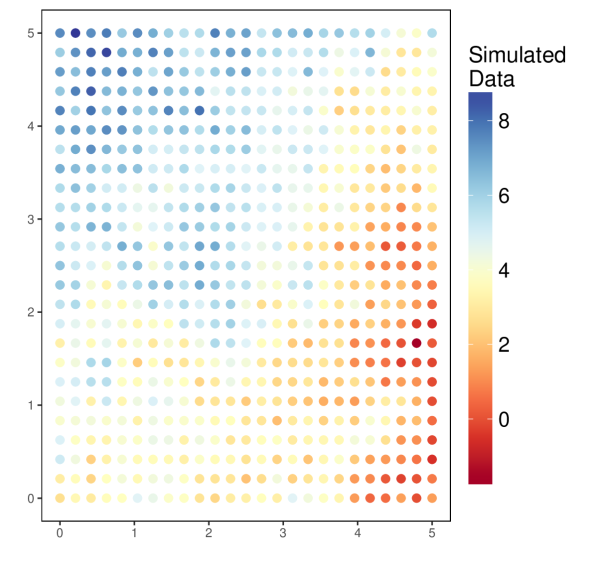
Figure 1: Left: true mixture component ellipses with observation locations (red) and validation locations (green). Right: simulated data.

The simdata object includes sim.locations, the simulated data locations; mc.locations, the mixture component locations; mc.kernels, the true mixture component kernel matrices; sim.data, the simulated data; and holdout.index, a vector of the 60 randomly sampled validation location indices. Note that there are actually ten independent and identically distributed replicates of the data contained in the ten columns of sim.data; in what follows the first column of data will be used.

Figure 1 can be created with

R> plot( simdata$mc.locations,pch="+",asp=1.25,xlab="",+ylab="",xlim=c(-0.5,5.5),cex=2,col="#4575b4",main="")R>points(simdata$sim.locations[ -simdata$holdout.index,],col="#d73027",+pch="+")R>points(simdata$sim.locations[ simdata$holdout.index,],col="#5aae61")R>for(iin1:dim(simdata$mc.locations )[1] ) + lines( ellipse( simdata$mc.kernels[,,i],+centre=simdata$mc.locations[ i, ], level = 0.5 ) ) R> ggplot( data.frame( simdata = simdata$sim.data[,1],+xcoord=simdata$sim.locations[ , 1 ], + ycoord = simdata$sim.locations[,2]),+aes(x=xcoord,y=ycoord,color=simdata))++coord_{f}ixed(ratio=1.25)+geom_{p}oint(size=2.5)++xlab("")+ylab("")+name="Simulated\nData")++scale_{c}olor_{g}radientn(colours=brewer.pal(11,"RdYlBu"),+theme(panel.background=element_{r}ect(fill="white"),+panel.border=element_{r}ect(colour="black",fill=NA),+panel.grid=element_{b}lank(),legend.key.height=unit(2,"cm"),+legend.title=element_{t}ext(size=16),+legend.text=element_{t}ext(size=15))\par\noindent(Note:thiscoderequiresthe\pkg{ggplot2}({\cite[citep]{\@@bibref{AuthorsPhrase1Year}{R_ggplot2}{\@@citephrase{, }}{}}}),\pkg{RColorBrewer}({\cite[citep]{\@@bibref{AuthorsPhrase1Year}{R_RColorBrewer}{\@@citephrase{, }}{}}}),and\pkg{ellipse}({\cite[citep]{\@@bibref{AuthorsPhrase1Year}{R_ellipse}{\@@citephrase{, }}{}}})packagesin\proglang{R}.)\par$

6.1 Selection of fixed components in the model

In order to fit the nonstationary model, the user must specify three components: (1) the number and placement of mixture component locations, (2) the fitting radius $r$, and (3) the tuning parameter $\lambda_{w}$. For this simulated data set, the true number and placement of the mixture component locations as well as the tuning parameter are known, and these true values will be used. However, even for the simulated data, an optimal fit radius is not known. When the tuning parameter is unknown the package provides a default value, but this may or may not be the optimal choice.

Given that the nonstationary model can be fit relatively quickly for given values of $r$, a recommended strategy is to fit the model many times for a variety of different values (same for the mixture component grid and $\lambda_{w}$, when these are unknown) and choose the final values based on which combination yields the “best” results. Of course, there is a trade-off between choices of the mixture component grid and fit radius: for a particular grid, the radius should be chosen such that a reasonable number of data points are used to fit each locally stationary model. It is here that the mc_N function may be helpful, because the user can quickly determine how many locations fall within the fitting radius of each grid point. For example, using the simulated data: R> mc_N( coords = simdata$sim.locations[-simdata$holdout.index, ], + mc.locations = simdata$mc.locations,fit.radius=2)[1]164212165209269212153204157Thatis,usingthetruemixturecomponentgridandafitradiusof$r=2$,thelocalmodelswillbefitusinganywherefrom157to269datapoints.\par Forthesimulateddatainthisapplication,the``best^{\prime\prime}fitwaschosenbasedonthequalityoftheanisotropyparameterestimatesrelativetothetruevalues;inothercasesnotinvolvingsimulateddata,``best^{\prime\prime}mightbedefinedintermsofthecross-validationcriteria(see,e.g.,Section\ref{USprecip}).Thevaluesusedforthesethreecomponentsinthefinalfit(Section\ref{final_sim})werethetruemixturecomponentgrid(with$K=9$evenlyspacedlocationsoverthedomain),afitradiusof$r=2.3$units,andthetruetuningparametervalueof$λ_w = 2.

6.2 Final model fitting

Using the final choices of the fixed model components, the nonstationary model can be fit to the non-hold-out data (and results summarized) by

R> NSfit.model <- NSconvo_fit( + coords = simdata$sim.locations[-simdata$holdout.index, ], + data = simdata$sim.data[-simdata$holdout.index, 1 ], + cov.model = "exponential", fit.radius = 2.3, lambda.w = 2, + mc.locations = simdata$mc.locations,+mean.model=simdata$sim.data[ -simdata$holdout.index,1]+~{}simdata$sim.locations[ -simdata$holdout.index,1]++simdata$sim.locations[ -simdata$holdout.index,2])R>summary(NSfit.model)Similarly,theanisotropicmodelcanbefittothenon-hold-outdata(andresultssummarized)byR>anisofit.model<-Aniso{}_{f}it(+coords=simdatasim.locations[-simdataholdout.index,],+data=simdatasim.data[-simdataholdout.index,1],+cov.model=\mathrm{"}exponential\mathrm{"},+mean.model=simdatasim.data[-simdataholdout.index,1]+simdatasim.locations[-simdataholdout.index,1]++simdatasim.locations[-simdataholdout.index,2])R>summary(anisofit.model)\text{Table 1Table 11Table 1True valueStationary modelNonstationary modelβ0 (intercept)44.0393.905β1 (x-coordinate)-0.5-0.695-0.678β2 (y-coordinate)0.50.7410.770τ2 (nugget)0.10.0860.107σ2 (variance)11.0380.958CRPS–-0.424-0.415MSPE–0.5460.5241Param}$