Expansion potentials for exact far-from-equilibrium spreading of particles and energy

Abstract

The rates at which energy and particle densities move to equalize arbitrarily large temperature and chemical potential differences in an isolated quantum system have an emergent thermodynamical description whenever energy or particle current commutes with the Hamiltonian. Concrete examples include the energy current in the 1D spinless fermion model with nearest-neighbor interactions (XXZ spin chain), energy current in Lorentz-invariant theories or particle current in interacting Bose gases in arbitrary dimension. Even far from equilibrium, these rates are controlled by state functions, which we call “expansion potentials”, expressed as integrals of equilibrium Drude weights. This relation between nonequilibrium quantities and linear response implies non-equilibrium Maxwell relations for the Drude weights. We verify our results via DMRG calculations for the XXZ chain.

The dynamics of how a system of interacting particles expands from an initial state with spatial variation of temperature, density, or both is one of the basic problems in non-equilibrium statistical physics. The study of quantum effects on this process was reinvigorated by the experimental creation of ultracold atomic gases Bloch et al. (2008); Lamacraft and Moore (2012), including cases where the atoms are confined to one or two spatial dimensions. Originally the main quantity measured was the momentum distribution Paredes et al. (2004); Kinoshita et al. (2006), but recent progress on the “quantum gas microscope” and related techniques has made it possible to image particle density with high resolution, e.g., on single sites of an optical lattice Bakr et al. (2009); Gemelke et al. (2009); Sherson et al. (2010).

Such imaging methods mean that important observables to characterize expansion of an atomic gas in either free space or an optical lattice Ronzheimer et al. (2013) are not the same as those for non-equilibrium processes in electronic transport. For electrons, the charge or energy current between two leads has been studied in hundreds of situations, including a few non-equilibrium results with interactions such as tunneling between Luttinger liquids Kane and Fisher (1992); Fendley et al. (1995), the interacting resonant level model Doyon (2007); Boulat and Saleur (2008); Boulat et al. (2008); Freton and Boulat (2014) and the single impurity Anderson model (for a recent review see Eckel et al. (2010)). The point of the present work is to show that one natural quantity of interest for atomic expansion measurements Morsch et al. (2002); Strohmaier et al. (2007); Gerbier et al. (2008); Hackermüller et al. (2010); Hung et al. (2010); Schneider et al. (2012), namely the change in time of the first moment of particle or energy density, has a precise non-equilibrium thermodynamic description in a broad class of systems. For a continuum system with either Lorentz or Galilean invariance, this description reduces to standard thermodynamic state functions, but we find that even lattice systems relevant to current experiments have a description in terms of an “expansion potential” that is distinct from conventional thermodynamic quantities.

We use this description to compute the energy expansion rate exactly in the anisotropic Heisenberg spin chain (XXZ model) and compare our results in detail against time-dependent density-matrix renormalization group (DMRG White and Feiguin (2004); Zwolak and Vidal (2004); Schollwoeck (2011)) calculations using the finite temperature algorithm explained in Karrasch et al. (2013a). The same formalism is applicable to higher-dimensional systems with emergent Lorentz or Galilean invariance. Our predictions apply in particular to a one-dimensional Bose gas (Lieb-Liniger model Lieb and Liniger (1963); Yang (1967), or its lattice regularization in terms of $q$-deformed bosons Bogoliubov and Bullough (1992)), expanding into vacuum, a problem that has attracted a lot of attention recently Castin and Dum (1996); Kagan et al. (1996); Pedri et al. (2003); Gangardt and Pustilnik (2008); Muth et al. (2010); Caux and Konik (2012); Rigol et al. (2007); Gritsev et al. (2010); Caux and Essler (2013); Iyer and Andrei (2012); Ronzheimer et al. (2013); Campbell et al. (2015); Karrasch et al. (2014). Our results show that, at least for some quantities, exact results can be obtained for far-from-equilibrium expansion even in lattice models at arbitrary coupling strength.

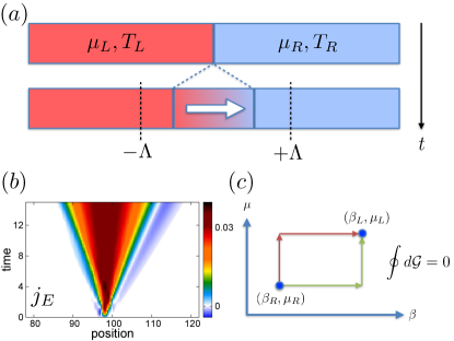
Figure 1: (a) Nonequilibrium expansion setup considered in this letter. (b) Energy point current $j_{E}(x,t)$ in the XXZ spin chain (see Fig 2 for parameters). (c) The variation of the expansion potential ${\cal G}$ does not depend on the path in the $(\beta,\mu)$ space. This implies nonequilibrium Maxwell relations (see text).

At $t=0$, prepare two semi-infinite regions $x<0$ and $x>0$ at equilibrium with chemical potentials and temperatures $(\mu_{L},T_{L})$ and $(\mu_{R},T_{R})$ (Fig 1a). (The initial state on the boundary between the two leads, or a possible finite extent of the boundary region, will not matter for the quantities of interest here after some initial transient.) We write one-dimensional equations for simplicity but the concept is general. We quantify the expansion for $t>0$ by the time dependence of the first moment of particle density, or similarly for energy,

$$M_{1}(t)=\int^{\Lambda}_{-\Lambda}\,n(x,t)x\,dx,$$ (1)

with $\Lambda$ a large observation scale: $\Lambda\gg vt$ with $v$ a typical velocity. From now on we suppress the arguments of $n$ and $M_{1}$. The continuity equation relates density and current $\partial_{t}n+\partial_{x}j=0$. Now $\frac{dM_{1}}{dt}=-\int^{\Lambda}_{-\Lambda}\,x\partial_{x}j\,dx={\cal J}$, with ${\cal J}=\int^{\Lambda}_{-\Lambda}j\,dx$ where in the integration by parts we have assumed $j(x)\approx 0$ at $x=\pm\Lambda$ (Fig 1b).

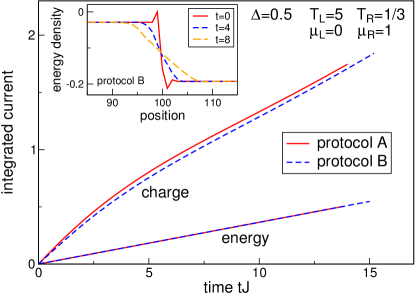
Figure 2: Spatially integrated charge and energy currents in the XXZ model with open boundary conditions as a function of time for one choice of parameters $T_{L}$, $\mu_{L}$, $T_{R}$, $\mu_{R}$ at $\Delta=0.5$ under two protocols (A) and (B) that differ only in the way the central bond is dealt with in the initial state Sup . The currents ${\cal J}=\int^{\Lambda}_{-\Lambda}jdx$ are locally integrated around the cut site. The chemical potentials $\mu_{L,R}$ prepare the state but are not included in the real-time evolution (i.e., they are chemical potentials rather than electric potentials). Inset: energy density profile as a function of time. The spatially integrated energy current is equal to $dM^{\rm th}_{1}/dt$ where $M^{\rm th}_{1}$ is the first moment of energy density.

The key ingredient for the existence of an expansion potential is the conservation of integrated current:

$$\left[\oint j\,dx,H\right]=0,$$ (2)

which is true for many problems of interest with periodic boundary conditions. Note that this is a stronger statement than what is sometimes meant by a “conserved current”, which is anything related to a conserved charge by a continuity equation. A simple example with such a conservation law is a Bose gas in $d$ spatial dimensions with say, $\delta$-function interactions $H=\int d^{d}x\Psi^{\dagger}\left(-\frac{\nabla^{2}}{2m}\right)\Psi+c\Psi^{\dagger}\Psi^{\dagger}\Psi\Psi$, with $\left[\Psi^{\dagger}(x),\Psi(y)\right]=\delta(x-y)$, where the total particle current ${\cal J}_{Q}=-i\int dx(\Psi^{\dagger}\nabla\Psi-\nabla\Psi^{\dagger}\Psi)$ is conserved. More generally, a system with one species of particles moving in the continuum in any spatial dimension will satisfy (2) for particle current if particle current is proportional to total momentum and momentum is conserved by the interactions. A less trivial example of (2) is energy current in the spinless fermion model or XXZ spin chain (we will use the former representation): the energy current operator ${\cal J}_{E}=i\sum_{j}[h_{j},h_{j+1}]$ commutes with the XXZ Hamiltonian $H^{\rm XXZ}=\sum_{i}h_{i}$ with

$$h_{i}=-\frac{J}{2}\left(c_{i+1}^{\dagger}c_{i}+{\rm h.c.}\right)+J\Delta\left(n_{i}-\frac{1}{2}\right)\left(n_{i+1}-\frac{1}{2}\right),$$ (3)

with $n_{i}=c_{i}^{\dagger}c_{i}$, implying purely ballistic energy transport Schwab et al. (2000); Sup . An example of a current not conserved in this sense is charge current in the XXZ model; while there is a degree of ballistic transport in this model in the gapless regime even at nonzero temperature Prosen (2011); Karrasch et al. (2012, 2013b), the commutator in (2) is nonzero. Steady-state energy currents between reservoirs have been actively studied Sotiriadis and Cardy (2008); Bernard and Doyon (2012); Karrasch et al. (2013c); Bernard and Doyon (2015); Doyon (2015); De Luca et al. (2014); Bhaseen et al. (2015) but exact results have been difficult to obtain except in the low-temperature conformal limit or for noninteracting systems.

Expansion potentials.

The global current conservation law (2) implies that the current density should itself satisfy a continuity equation for some “current of current” $P$,

$$\partial_{t}j+\partial_{x}P=0,$$ (4)

and we will see in the following that the operator $P$ is related to pressure for systems with emergent Galilean or Lorentz invariance. Now spatially integrate this second continuity equation (4) over the region $[-\Lambda,\Lambda]$ centered on the boundary between our two large reservoirs $L$ and $R$. Then

$$\frac{d^{2}M_{1}}{dt^{2}}=-P\large]^{\Lambda}_{-\Lambda}=\Delta{\cal G}={\cal G}_{L}-{\cal G}_{R},$$ (5)

where we have introduced the expansion potential ${\cal G}(\mu,T)=\langle P\rangle_{\mu,T}$ for the thermodynamic expectation of the operator $P$.

This is a strong constraint on the integrated current ${\cal J}=\int_{-\Lambda}^{\Lambda}jdx$. We perform DMRG calculations on a XXZ spin chain with open boundary conditions that effectively describes a region of an infinite system. Within that region (shown in Fig. 1b), the total energy current is clearly not conserved Sup and grows linearly with time (Fig. 2) for times short enough that the reservoirs are effectively infinite, so their initial values can be used in the boundary evaluation on the right-hand side of (5). If the current has both diffusive and ballistic components (like the charge current in the XXZ chain), diffusive contributions die out after a transient and the spatially integrated current also grows linearly. However, the situation becomes especially simple for a current satisfying (2), the key being that the right-hand side of (5) contains only the operator $P$ evaluated at equilibrium, since deep within the reservoirs the system remains arbitrarily close to equilibrium in this intermediate time regime. This result relies only on (2) and does not depend on whether the system is gapped or gapless for instance.

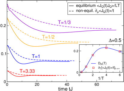
Figure 3: Comparison between charge Drude weight (long-time asymptote of $\langle{\cal J}_{Q}(t){\cal J}_{Q}(0)\rangle/LT$ and rate of particle spreading $d^{2}M^{\rm c}_{1}/dt^{2}=\langle{\cal J}_{Q}(t)\rangle_{t}/t$ for a small chemical potential difference ($\Delta\mu\sim 10^{-3}\ll J=1$) in the XXZ chain (protocol A). Inset: similar relation for energy transport between thermal Drude weight and rate of energy spreading $d^{2}M^{\rm th}_{1}/dt^{2}=\langle{\cal J}_{E}(t)\rangle_{t}/t$ for a small temperature difference at half-filling (see eq. (6)).

Linear response.

One more relation is all that is needed to compute the expansion potential in some important cases. This is because eq. (5) implies that linear-response is enough to predict non-equilibrium, since linear response gives the derivative of ${\cal G}$, and knowing its derivative determines the function up to an arbitrary additive constant. Focusing for the moment on energy current and a purely thermal gradient, linear response then predicts $j_{E}=-\sigma_{E}\nabla T$ with the thermal conductivity characterized by a thermal Drude weight $\sigma_{E}(\omega)=\pi D_{\rm th}(T)\delta(\omega)$ with $D_{\rm th}=\beta^{2}\langle{\cal J}_{E}^{2}\rangle/L$, where $L$ is the size of the system. The spatially integrated current between the two reservoirs $R$ and $L$ then reads $\int_{-\Lambda}^{\Lambda}j_{E}dx=\pi\Delta T\delta(\omega=0)D_{\rm th}(T)$ where the time $t$ can be thought of as an infrared cutoff that regularizes $\delta(\omega=0)\approx\int^{t}_{-t}\frac{dt}{2\pi}=t/\pi$. We thus find

$$\frac{d^{2}M^{\rm th}_{1}}{dt^{2}}=\frac{1}{t}\langle{\cal J}_{E}\rangle_{t}=D_{\rm th}(T)\times(\Delta T),$$ (6)

with ${\cal J}_{E}=\int_{-\Lambda}^{\Lambda}j_{E}dx$ and $\langle\dots\rangle_{t}$ refers to the nonequilibrium expectation value after time $t$. For the charge current at constant temperature $T_{R}=T_{L}=T$, we similarly find $\frac{d^{2}M^{\rm c}_{1}}{dt^{2}}=\langle{\cal J}_{Q}\rangle_{t}/t=D_{c}\Delta\mu$ with the charge Drude weight $D_{c}=\beta\langle{\cal J}_{Q}^{2}\rangle/L$ (if $[H,{\cal J}_{Q}]=0$), for a small chemical potential gradient $\Delta\mu$. These results are easily extended to the case where both temperature and chemical potential gradients are present (see below). We also note that these linear response results remain valid even if the currents are not fully conserved and contain diffusive parts, like the charge current in the XXZ spin chain, which provides a direct way to measure Drude weights via imaging in cold atom experiments (see also Hazlett et al. (2013)). We checked this relation between charge (resp. thermal) Drude weight and linear-response rate of spreading of charge (resp. energy) in the XXZ chain (see Fig. 3) – similar relations also exist for diffusive systems Liu et al. (2014).

Nonequilibrium expansion potentials.

The thermodynamic description eq. (5) together with the linear response prediction implies that the spreading of particles and energy far from equilibrium are fully characterized by the equilibrium Drude weights. As an example, let us consider the rate of energy spread in the XXZ spin chain between two reservoirs at different temperatures $T_{R}$ and $T_{L}$ and $\mu=0$. Then even far from equilibrium

$$\frac{dM^{\rm th}_{1}}{dt}\underset{t\to\infty}{\sim}t\times\int_{T_{R}}^{T_{L}}D_{\rm th}(T)dT.$$ (7)

In other words, the nonequilibrium rate of energy spread is given by the variation $\Delta_{R\to L}{\cal G}_{E}={\cal G}_{E}(T_{L})-{\cal G}_{E}(T_{R})$ of a state function ${\cal G}_{E}(T)$ with $\partial_{T}{\cal G}_{E}=D_{\rm th}(T)$. This can be checked numerically by comparing the rate of expansion to the thermal Drude weight of the XXZ model computed by Klümper and Sakai Klümper and Sakai (2002) (see Fig. 4).

This is easily generalized to the case of reservoirs $R$ and $L$ with both different temperatures ($T_{R}$ and $T_{L}$) and chemical potentials ($\mu_{R}$ and $\mu_{L}$) . If the energy current is conserved, eq. (5) implies that the far-from-equilibrium rate of energy spread is given by the variation of an expansion potential ${\cal G}_{E}(\mu,\beta=T^{-1})$

$$\frac{d^{2}M^{\rm th}_{1}}{dt^{2}}=\Delta_{R\to L}{\cal G}_{E}=\int_{R\to L}d{\cal G}_{E},$$ (8)

where the differential $d{\cal G}_{E}$ is exact so that the integral does not depend on the chosen path. The state function ${\cal G}_{E}$ is then fully determined by the equilibrium Drude weights associated with the conservation of the energy current. Linear response theory Mahan (1990) then yields

$$d{\cal G}_{E}=\beta\frac{\langle{\cal J}_{Q}{\cal J}_{E}\rangle}{L}d\mu-\left(\frac{\langle{\cal J}_{E}^{2}\rangle}{L}-\mu\frac{\langle{\cal J}_{Q}{\cal J}_{E}\rangle}{L}\right)d\beta.$$ (9)

Even if ${\cal J}_{Q}$ is not conserved, the Drude thermopower is a thermodynamic quantity determined by $\langle{\cal J}_{Q}{\cal J}_{E}\rangle$ provided that $\left[{\cal J}_{E},H\right]=0$. If the particle current is conserved, we find similarly that the integrated nonequilibrium particle current between two reservoirs $(\mu_{R},\beta_{R})$ and $(\mu_{L},\beta_{L})$ is given by the variation of another state function $\frac{d^{2}M^{\rm c}_{1}}{dt^{2}}=\Delta_{R\to L}{\cal G}_{Q}$ with $d{\cal G}_{Q}=\beta\frac{\langle{\cal J}_{Q}^{2}\rangle}{L}d\mu-\left(\frac{\langle{\cal J}_{Q}{\cal J}_{E}\rangle}{L}-\mu\frac{\langle{\cal J}_{Q}^{2}\rangle}{L}\right)d\beta$.

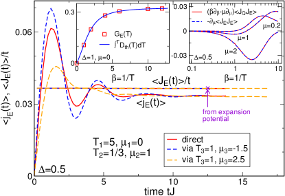
Figure 4: The thermodynamic description (5) implies that the spatially integrated current ${\cal J}_{1\to 2}$ between two reservoirs $1$ and $2$ should be equal to ${\cal J}_{1\to 3}+{\cal J}_{3\to 2}$ for any intermediate reservoir 3. We verified this “cyclic invariance” of the spatially integrated energy current $\langle{\cal J}_{E}(t)\rangle_{t}/t$ and point current $\langle j_{E}(x=0,t)\rangle_{t}$ in the XXZ chain (protocol A). While cyclicity for the point current may be only approximate, it is exact for the integrated current. Insets: numerical check of eq. (7) and of the nonequilibrium Maxwell relation (10) that follows from conservation of energy current.

Nonequilibrium Maxwell relations.

We saw above that when either the energy or particle current is fully conserved, then even far from equilibrium the expansion dynamics of energy or particle densities are characterized by state functions that are entirely determined by equilibrium Drude weights. An interesting corollary of the path-independence of these state functions (Fig 1c) are nonequilibrium Maxwell relations for the Drude weights. For example, if the energy current is conserved, $\partial_{\mu}\partial_{\beta}{\cal G}_{E}=\partial_{\beta}\partial_{\mu}{\cal G}_{E}$ yields

$$(\beta\partial_{\beta}-\mu\partial_{\mu})\langle{\cal J}_{Q}{\cal J}_{E}\rangle+\partial_{\mu}\langle{\cal J}_{E}^{2}\rangle=0,$$ (10)

which can also be rewritten as $\langle\Delta H{\cal J}_{Q}{\cal J}_{E}\rangle=\langle\Delta N{\cal J}_{E}^{2}\rangle$ with $\Delta H=H-\langle H\rangle$ and $\Delta N=N-\langle N\rangle$. This equality was known in the context of the XXZ chain Louis and Gros (2003) and was actually used to compute the Drude thermopower analytically Sakai and Klümper (2005), but our approach provides a very transparent derivation of why such a relation has to hold (see Fig. 4 for a numerical check). If the charge current is conserved, then the associated nonequilibrium Maxwell relation reads $(\beta\partial_{\beta}-\mu\partial_{\mu})\langle{\cal J}_{Q}^{2}\rangle+\partial_{\mu}\langle{\cal J}_{E}{\cal J}_{Q}\rangle=0$, which can also be rewritten as $\langle\Delta H{\cal J}_{Q}^{2}\rangle=\langle\Delta N{\cal J}_{Q}{\cal J}_{E}\rangle$.

Examples in $d>1$ dimensions.

Even though most of the arguments discussed above focused on one dimension for simplicity, the general concepts apply in higher dimension as well. For a system with emergent Lorentz symmetry ($z=1$ critical points for instance), the symmetry of the stress-energy tensor means that the energy current $T_{0i}$ with $i=1,\dots,d$ is also the (conserved) momentum density $T_{i0}$. The energy expansion potential then reads ${\cal G}_{E}(\beta)=-\int^{\beta}\,d\beta\int d^{d}x\frac{1}{d}\sum_{i}\langle T_{0i}(x)T_{0i}(0)\rangle$, which can be related to pressure Doyon (2015); Bhaseen et al. (2015). In a non-relativistic system with a single species of particles and current proportional to (conserved) momentum, there is a particle expansion potential; the interacting Bose gas is one such example. The particle Drude weight $D_{c}$ is then entirely determined by the sum rule $\int\frac{d\omega}{\pi}\sigma(\omega)=D_{c}=\frac{n}{m}$ with $n$ the density and $m$ the mass Mahan (1990). This immediately implies that the expansion potential is simply related to pressure ${\cal G}_{Q}=-\frac{\Omega}{Vm}=\frac{P}{m}$ with $\Omega$ the thermodynamic grand potential and $V$ the volume – this is a consequence of Galilean invariance . The Drude thermopower is then given by $\langle{\cal J}_{Q}{\cal J}_{E}\rangle/V=\frac{T}{m}(u+P)$ with $u$ the internal energy density. These quantities can be computed explicitly for the Lieb-Liniger gas in one dimension as a function of $T$ and $\mu$ (or particle density) Yang and Yang (1969). This and other simple cases where the expansion potentials can be computed explicitly, such as non-interacting systems and Luttinger liquids, are given in Supplemental Material Sup .

Nature of the steady-state.

Interestingly, the variation of expansion potential $\Delta{\cal G}$ provides a lower bound for the point current $j(x)$ Doyon (2015). However, the more general relation between spatially integrated and point currents remains mysterious. We find numerically that both the energy density $n_{E}(x,t)$ and the energy current $j_{E}(x,t)$ in the XXZ spin chain at half-filling become functions of $x/t$ at large enough times, with nontrivial limiting shapes Sup . In the low-temperature limit described by conformal field theory Bernard and Doyon (2012, 2015), we expect a uniform steady-state local current $j_{E}(x)=\frac{\Delta{\cal G}}{2v}=\frac{\pi}{12}(T_{L}^{2}-T_{R}^{2})$ over a region of size $2vt$ with $v$ the spinon velocity. However, we find that the rescaled functions $j_{E}(x/t)$, $n_{E}(x/t)$ even at moderate temperatures are very far from that picture: in general, there is no nonzero range of the reduced variable $x/t$ for which $j_{E}(x/t$) is constant, indicating that the steady-state region spreads sub-ballistically, and there are no transient “shock-waves” like those expected in the presence of Lorentz invariance Bhaseen et al. (2015); Bernard and Doyon (2015) separating the uniform steady-state region from the reservoirs. It is an interesting problem for future work to determine more properties of the limiting function $j_{E}(x/t)$, possibly by adapting the recently developed hydrodynamic approaches for relativistic systems Bhaseen et al. (2015); Bernard and Doyon (2015) to incorporate the additional conserved quantities of integrable lattice spin chains.

Discussion.

In closing, we emphasize that the expansion potentials generalize familiar concepts in the presence of either Galilean or Lorentz invariance to considerably more complex physical situations. Lattice models for which a current is conserved in the sense of (2) include the XYZ spin chain, the $q$-Bose gas Bogoliubov and Bullough (1992), and the supersymmetric point of the $t$-$J$ model Essler and Korepin (1992). For systems where the conservation law does not strictly hold, such as the Bose-Hubbard model at small occupancy where rare double occupancies spoil the mapping to the XXZ model, Joule heating and other strongly non-equilibrium physics could be computed using perturbation theory from the expansion-potential case. It would be interesting to connect the expansion potential to other nonequilibrium effects, such as “quantum quenches” of a coupling Calabrese and Cardy (2006), which can reveal topological phases Sengupta et al. (2008); Vasseur et al. (2014). For lattice models with conserved energy current but without full integrability, the expansion potential still exists and could be computed numerically at equilibrium, while it would serve as a useful constraint on predictions about far-from-equilbrium energy flow Bernard and Doyon (2015).

See pages 1 of NonequilibriumExpansionSupplement.pdf

See pages 2 of NonequilibriumExpansionSupplement.pdf

See pages 3 of NonequilibriumExpansionSupplement.pdf

See pages 4 of NonequilibriumExpansionSupplement.pdf

See pages 5 of NonequilibriumExpansionSupplement.pdf

See pages 6 of NonequilibriumExpansionSupplement.pdf

References

- Bloch et al. (2008) I. Bloch, J. Dalibard, and W. Zwerger, Rev. Mod. Phys. 80, 885 (2008).
- Lamacraft and Moore (2012) A. Lamacraft and J. Moore, Potential insights into non-equilibrium behavior from atomic physics (Elsevier, Amsterdam, 2012) pp. 177–202, in Ultracold Bosonic and Fermionic Gases, edited by A. Fetter, K. Levin, and D. Stamper-Kurn.
- Paredes et al. (2004) B. Paredes, A. Widera, V. Murg, O. Mandel, S. Folling, I. Cirac, G. V. Shlyapnikov, T. W. Hansch, and I. Bloch, Nature 429, 277 (2004).
- Kinoshita et al. (2006) T. Kinoshita, T. Wenger, and D. Weiss, Nature 440, 900 (2006).
- Bakr et al. (2009) W. S. Bakr, J. I. Gillen, A. Peng, S. Folling, and M. Greiner, Nature 462, 74 (2009).
- Gemelke et al. (2009) N. Gemelke, X. Zhang, C.-L. Hung, and C. Chin, Nature 460, 995 (2009).
- Sherson et al. (2010) J. F. Sherson, C. Weitenberg, M. Endres, M. Cheneau, I. Bloch, and S. Kuhr, Nature 467, 68 (2010).
- Ronzheimer et al. (2013) J. P. Ronzheimer, M. Schreiber, S. Braun, S. S. Hodgman, S. Langer, I. P. McCulloch, F. Heidrich-Meisner, I. Bloch, and U. Schneider, Phys. Rev. Lett. 110, 205301 (2013).
- Kane and Fisher (1992) C. Kane and M. Fisher, Phys. Rev. Lett. 68, 1220 (1992).
- Fendley et al. (1995) P. Fendley, A. Ludwig, and H. Saleur, Phys. Rev. B 52, 8934 (1995).
- Doyon (2007) B. Doyon, Phys. Rev. Lett. 99, 076806 (2007).
- Boulat and Saleur (2008) E. Boulat and H. Saleur, Phys. Rev. B 77, 033409 (2008).
- Boulat et al. (2008) E. Boulat, H. Saleur, and P. Schmitteckert, Phys. Rev. Lett. 101, 140601 (2008).
- Freton and Boulat (2014) L. Freton and E. Boulat, Phys. Rev. Lett. 112, 216802 (2014).
- Eckel et al. (2010) J. Eckel, F. Heidrich-Meisner, S. G. Jakobs, M. Thorwart, M. Pletyukhov, and R. Egger, New Journal of Physics 12, 043042 (2010).
- Morsch et al. (2002) O. Morsch, M. Cristiani, J. H. Müller, D. Ciampini, and E. Arimondo, Phys. Rev. A 66, 021601 (2002).
- Strohmaier et al. (2007) N. Strohmaier, Y. Takasu, K. Günter, R. Jördens, M. Köhl, H. Moritz, and T. Esslinger, Phys. Rev. Lett. 99, 220601 (2007).
- Gerbier et al. (2008) F. Gerbier, S. Trotzky, S. Fölling, U. Schnorrberger, J. D. Thompson, A. Widera, I. Bloch, L. Pollet, M. Troyer, B. Capogrosso-Sansone, N. V. Prokof’ev, and B. V. Svistunov, Phys. Rev. Lett. 101, 155303 (2008).
- Hackermüller et al. (2010) L. Hackermüller, U. Schneider, M. Moreno-Cardoner, T. Kitagawa, T. Best, S. Will, E. Demler, E. Altman, I. Bloch, and B. Paredes, Science 327, 1621 (2010).
- Hung et al. (2010) C.-L. Hung, X. Zhang, N. Gemelke, and C. Chin, Phys. Rev. Lett. 104, 160403 (2010).
- Schneider et al. (2012) U. Schneider, L. Hackermuller, J. P. Ronzheimer, S. Will, S. Braun, T. Best, I. Bloch, E. Demler, S. Mandt, D. Rasch, and A. Rosch, Nat Phys 8, 213 (2012).
- White and Feiguin (2004) S. R. White and A. Feiguin, Phys. Rev. Lett. 93, 076401 (2004).
- Zwolak and Vidal (2004) M. Zwolak and G. Vidal, Phys. Rev. Lett. 93, 207205 (2004).
- Schollwoeck (2011) U. Schollwoeck, Annals of Physics 326, 96 (2011), january 2011 Special Issue.
- Karrasch et al. (2013a) C. Karrasch, J. H. Bardarson, and J. E. Moore, New Journal of Physics 15, 083031 (2013a).
- Lieb and Liniger (1963) E. Lieb and W. Liniger, Physical Review 130, 1605 (1963).
- Yang (1967) C. N. Yang, Phys. Rev. Lett. 19, 1312 (1967).
- Bogoliubov and Bullough (1992) N. M. Bogoliubov and R. K. Bullough, Journal of Physics A: Mathematical and General 25, 4057 (1992).
- Castin and Dum (1996) Y. Castin and R. Dum, Phys. Rev. Lett. 77, 5315 (1996).
- Kagan et al. (1996) Y. Kagan, E. L. Surkov, and G. V. Shlyapnikov, Phys. Rev. A 54, R1753 (1996).
- Pedri et al. (2003) P. Pedri, L. Santos, P. Öhberg, and S. Stringari, Phys. Rev. A 68, 043601 (2003).
- Gangardt and Pustilnik (2008) D. M. Gangardt and M. Pustilnik, Phys. Rev. A 77, 041604 (2008).
- Muth et al. (2010) D. Muth, B. Schmidt, and M. Fleischhauer, New Journal of Physics 12, 083065 (2010).
- Caux and Konik (2012) J.-S. Caux and R. M. Konik, Phys. Rev. Lett. 109, 175301 (2012).
- Rigol et al. (2007) M. Rigol, V. Dunjko, V. Yurovsky, and M. Olshanii, Phys. Rev. Lett. 98, 050405 (2007).
- Gritsev et al. (2010) V. Gritsev, T. Rostunov, and E. Demler, Journal of Statistical Mechanics: Theory and Experiment 2010, P05012 (2010).
- Caux and Essler (2013) J.-S. Caux and F. H. L. Essler, Phys. Rev. Lett. 110, 257203 (2013).
- Iyer and Andrei (2012) D. Iyer and N. Andrei, Phys. Rev. Lett. 109, 115304 (2012).
- Campbell et al. (2015) A. S. Campbell, D. M. Gangardt, and K. V. Kheruntsyan, Phys. Rev. Lett. 114, 125302 (2015).
- Karrasch et al. (2014) C. Karrasch, J. E. Moore, and F. Heidrich-Meisner, Phys. Rev. B 89, 075139 (2014).
- (41) See Supplemental Material, which includes Refs. Shastry and Sutherland (1990); Kane and Fisher (1996); Kinoshita et al. (2004); Hofferberth et al. (2007); van Amerongen et al. (2008); Bortz (2006); Ranson et al. (2014), for a description of the protocols and boundary conditions, a brief review of ballistic transport, a calculation of the expansion potentials for various models, and a description of the steady-state region .
- Schwab et al. (2000) K. Schwab, E. A. Henriksen, J. M. Worlock, and M. L. Roukes, Nature 404, 974 (2000).
- Prosen (2011) T. Prosen, Phys. Rev. Lett. 106, 217206 (2011).
- Karrasch et al. (2012) C. Karrasch, J. H. Bardarson, and J. E. Moore, Phys. Rev. Lett. 108, 227206 (2012).
- Karrasch et al. (2013b) C. Karrasch, J. Hauschild, S. Langer, and F. Heidrich-Meisner, Phys. Rev. B 87, 245128 (2013b).
- Sotiriadis and Cardy (2008) S. Sotiriadis and J. Cardy, Journal of Statistical Mechanics: Theory and Experiment 2008, P11003 (2008).
- Bernard and Doyon (2012) D. Bernard and B. Doyon, Journal of Physics A: Mathematical and Theoretical 45, 362001 (2012).
- Karrasch et al. (2013c) C. Karrasch, R. Ilan, and J. E. Moore, Phys. Rev. B 88, 195129 (2013c).
- Bernard and Doyon (2015) D. Bernard and B. Doyon, Annales Henri Poincaré 16, 113 (2015).
- Doyon (2015) B. Doyon, Nuclear Physics B 892, 190 (2015).
- De Luca et al. (2014) A. De Luca, J. Viti, L. Mazza, and D. Rossini, Phys. Rev. B 90, 161101 (2014).
- Bhaseen et al. (2015) M. J. Bhaseen, B. Doyon, A. Lucas, and K. Schalm, Nat Phys 11, 509 (2015).
- Hazlett et al. (2013) E. L. Hazlett, L.-C. Ha, and C. Chin, ArXiv e-prints (2013), arXiv:1306.4018 [cond-mat.quant-gas] .
- Liu et al. (2014) S. Liu, P. Hänggi, N. Li, J. Ren, and B. Li, Phys. Rev. Lett. 112, 040601 (2014).
- Klümper and Sakai (2002) A. Klümper and K. Sakai, Journal of Physics A: Mathematical and General 35, 2173 (2002).
- Mahan (1990) G. D. Mahan, Many-Particle Physics, 2nd ed., Physics of Solids and Liquids (Springer US, 1990).
- Louis and Gros (2003) K. Louis and C. Gros, Phys. Rev. B 67, 224410 (2003).
- Sakai and Klümper (2005) K. Sakai and A. Klümper, Journal of the Physical Society of Japan 74, 196 (2005).
- Note (1) A technical condition for direct application of our results is that the reservoirs be uniform, rather than having a parabolic confining potential, but a precisely characterized uniform atomic trap has recently been achieved and used to probe expansion Gaunt et al. (2013); Gotlibovych et al. (2014).
- Yang and Yang (1969) C. N. Yang and C. P. Yang, Journal of Mathematical Physics 10, 1115 (1969).
- Bernard and Doyon (2015) D. Bernard and B. Doyon, ArXiv e-prints (2015), arXiv:1507.07474 [cond-mat.stat-mech] .
- Essler and Korepin (1992) F. H. L. Essler and V. E. Korepin, Phys. Rev. B 46, 9147 (1992).
- Calabrese and Cardy (2006) P. Calabrese and J. Cardy, Physical Review Letters 96, 136801 (2006).
- Sengupta et al. (2008) K. Sengupta, D. Sen, and S. Mondal, Physical review letters 100, 077204_1 (2008).
- Vasseur et al. (2014) R. Vasseur, J. P. Dahlhaus, and J. E. Moore, Phys. Rev. X 4, 041007 (2014).
- Shastry and Sutherland (1990) B. S. Shastry and B. Sutherland, Phys. Rev. Lett. 65, 243 (1990).
- Kane and Fisher (1996) C. L. Kane and M. P. A. Fisher, Phys. Rev. Lett. 76, 3192 (1996).
- Kinoshita et al. (2004) T. Kinoshita, T. Wenger, and D. S. Weiss, Science 305, 1125 (2004).
- Hofferberth et al. (2007) S. Hofferberth, I. Lesanovsky, B. Fischer, T. Schumm, and J. Schmiedmayer, Nature 449, 324 (2007).
- van Amerongen et al. (2008) A. H. van Amerongen, J. J. P. van Es, P. Wicke, K. V. Kheruntsyan, and N. J. van Druten, Phys. Rev. Lett. 100, 090402 (2008).
- Bortz (2006) M. Bortz, Journal of Statistical Mechanics: Theory and Experiment 2006, P08016 (2006).
- Ranson et al. (2014) A. Ranson, C. Chin, and K. Levin, New Journal of Physics 16, 113072 (2014).
- Gaunt et al. (2013) A. L. Gaunt, T. F. Schmidutz, I. Gotlibovych, R. P. Smith, and Z. Hadzibabic, Phys. Rev. Lett. 110, 200406 (2013).
- Gotlibovych et al. (2014) I. Gotlibovych, T. F. Schmidutz, A. L. Gaunt, N. Navon, R. P. Smith, and Z. Hadzibabic, Phys. Rev. A 89, 061604 (2014).