Sliding Hopf bifurcation in interval systems

Abstract

In this paper, the equivariant degree theory is used to analyze the occurrence of the Hopf bifurcation under effectively verifiable mild conditions. We combine the abstract result with standard interval polynomial techniques based on Kharitonov’s theorem to show the existence of a branch of periodic solutions emanating from the equilibrium in the settings relevant to robust control. The results are illustrated with a number of examples.

1 Introduction

Subject and goal. Many problems in population dynamics, neural networks, fluid dynamics, solid mechanics, elasticity, chemistry, mechanical and electrical engineering lead to studying the so-called Hopf bifurcation (more precisely, Poincaré-Andronov-Hopf bifurcation) in dynamical systems parameterized by a real parameter (see, for example, [39, 5, 20, 26, 34] and references therein). To be more specific, given a parameterized family

$$\dot{x}=f(\alpha,x),\qquad\alpha\in[\alpha_{-},\alpha_{+}],\;x\in\mathbb{R}^{d},$$ (1)

where $f:[\alpha_{-},\alpha_{+}]\times\mathbb{R}^{d}\to{\mathbb{R}}^{d}$ is a continuous map and $(\alpha,0)$ is a curve of trivial stationary solutions, the Hopf bifurcation is a phenomenon occurring when $\alpha$ crosses some critical value $\alpha_{o}$ (for which the linearization $D_{x}f(\alpha,0)$ admits a purely imaginary eigenvalue) and resulting in appearance of a branch of small amplitude periodic solutions near the curve $(\alpha,0)$. In his original work [23], E. Hopf studied system (1) under the following assumptions: (a) $f$ is analytic in both variables; (b) for $\alpha=\alpha_{o}$, exactly two complex conjugate characteristic roots $\mu(\alpha)$ and $\overline{\mu(\alpha)}$ intersect the imaginary axis (absence of multiple/resonant roots); (c) $\mu(0)\not=0$ (exclusion of steady-state bifurcation); and, (d) ${\rm Re}\,\mu^{\prime}(0)\not=0$ (transversality). Hopf’s theorem includes conditions for the occurrence of the bifurcation (i.e., the existence result) and conditions for stability of small cycles bifurcating from the stationary point. After this pioneering work, a substantial effort was made in order to relax conditions (a)–(d) (see, for example, [39, 5, 20, 26, 34, 13, 36] and references therein). One objective of this paper is to present an abstract result on the occurrence of the Hopf bifurcation in (1) under very mild (and effectively verifiable) hypotheses containing many known occurrence results as a particular case (cf. Theorem 3.2, Theorem 3.5 and Remark 3.6). It should be stressed that we do not study stability of bifurcating periodic solutions.

Our choice of the conditions on the nonlinearity $f$ and its derivative $D_{x}f(\alpha,0)$ is essentially determined by the following observations. In analysis and design, it is customary to deal with approximations of complex models that have some degree of uncertainty (one can think of the so-called nominal systems widely used in robust control; see, for example, [7]). Considering a model with uncertain parameters, one can expect that the entries of the matrix $D_{x}f(\alpha,0)$ belong to some known intervals of values rather than being represented by fixed numbers. This suggests to study the Hopf bifurcation phenomenon for a class of systems (1) where coefficients of the linearization are limited to known intervals. In this setting, the characteristic polynomial of $D_{x}f(\alpha,0)$ that defines the stability properties of the linearization also becomes an interval polynomial (see, for example, [7]). Importantly, this setting includes the scenario when the characteristic values of the linearization of a representative system (1) slide along the imaginary axis when the bifurcation parameter is varied (see Figure 1a).

Figure 1: (a) Given an $\alpha$-parametrized family of characteristic polynomials with unknown coefficients that are limited to some intervals, the dashed lines bound a corridor for the real part $\tau(\alpha)={\rm Re}\,\mu(\alpha)$ of an eigenvalue, while the solid line indicates a sliding scenario for some selector of the family. (b) Possible complex behavior of the branch of periodic solutions.

The main goal of the present paper is to propose a method for analysis of the occurrence of the Hopf bifurcation in the presence of such sliding.

As a matter of fact, the sliding phenomenon makes the problem non-local. Namely, it does not allow one to localize a bifurcation point on the basis of the knowledge of the linearization, that is based on the condition ${\rm Re}\,\mu(\alpha)=0$ (see Figure 1 a,b).

To study the Hopf bifurcation in this setting, one needs to deal with the whole interval of sliding that consists of potential bifurcation points. Thus, sliding is in sharp contrast to the transversality condition (d) above. At the same time, to the best of our knowledge, all the existing results on the occurrence of Hopf bifurcation identify explicitly a critical value of the parameter $\alpha$ at which Re $\mu(\alpha)$ changes its sign (for the least restrictive condition of this type, we refer to [36]). Some conditions for the existence of a branch of cycles that are non-local with respect to the parameter can be found in [29, 30, 31].

The simplest scenario which includes sliding and is covered by our results is the following. Suppose that system (1) has an equilibrium $x=0$ for all values of the parameter $\alpha\in[\alpha_{-},\alpha_{+}]$. Assume that the linearization $D_{x}f(\alpha,0)$ of the right hand side is invertible and has at most one pair of purely imaginary eigenvalues for any $\alpha\in[\alpha_{-},\alpha_{+}]$. Finally, assume that the zero equilibrium is hyperbolic for $\alpha=\alpha_{\pm}$ and the dimension of the stable manifold of the linearization of (1) at zero is different for $\alpha=\alpha_{-}$ and $\alpha=\alpha_{+}$. Then there is a Hopf bifurcation point on the interval $(\alpha_{-},\alpha_{+})$. Theorem 3.2 presented below also covers more complex scenarios including multiple and resonant eigenvalues of the linearization on the imaginary axis.

Method. In [23], the Hopf bifurcation in (1) was studied based on the series expansion of $f$. The further progress was related to the methods rooted in the singularity theory: assuming that the system satisfies several regularity and genericity conditions, one can combine the normal form classification with Center Manifold Theorem/averaging method/Lyapunov-Schmidt reduction. For a detailed exposition of these concepts and related techniques, we refer to [21, 20, 39].

Being very effective in the settings they are usually applied to, the singularity theory based methods meet difficulties if a setting is not regular/generic enough. For example, dynamical systems with hysteresis components admit linearization at the origin while any small neighborhood of the origin contains non-differentiability points which makes the Center Manifold Reduction impossible (see [4, 2, 9, 32, 33, 42, 35]) for details). As long as the stability of bifurcating solutions is not questioned, one can use homotopy theory based methods. Important steps in this direction were done in [1] (framed bordism theory), [13] (Fuller index), [36] (parameter functionalization method combined with the Leray-Schauder degree), to mention a few.

During the last twenty years the equivariant degree theory emerged in non-linear analysis (for the detailed exposition of this theory, including historical remarks, we refer to recent monographs [5, 26] and surveys [3, 6, 25]; for the prototypal invariants, see [14, 15, 18, 38]). The equivariant degree, being the main topological tool used in this paper, is an instrument that allows “counting” orbits of solutions to symmetric equations in the same way as the usual Brouwer degree does, but according to their symmetry properties. In particular, the equivariant degree theory has all the attributes allowing its application in non-smooth and non-generic equivariant settings related to equivariant dynamical systems having, in general, infinite dimensional phase spaces with lack of linear structure (cf. [4]). We refer to [26, 5] and references therein for the equivariant degree treatment of the (symmetric) Hopf bifurcation in different environments (see also [28]). In the present paper, we use the $S^{1}$-degree with one free parameter (see [5] for the axiomatic approach).

Theorem 3.7 below explicitly refers to the verification of stability properties of interval polynomials (cf. conditions (R3) and (R4)). Among very few results on the connection between perturbations of the coefficient and root locations, Kharitonov’s theorem ([27], see also [7, 22]) takes a firm position. To be more specific, V. L. Kharitonov showed that given a family of interval polynomials with real coefficients, it is necessary and sufficient to test just four canonically defined members of the family in order to decide that all polynomials are Hurwitz stable. The main topological ingredient of Kharitonov’s proof is the so-called Zero Exclusion Principle (in short ZEP) which can be traced back to the classical Argument principle in Complex Analysis. In this paper, combining ZEP with simple combinatorial arguments, we establish a Kharitonov type result for the so-called $k$-stable interval polynomials (cf. Lemma 2.4 and Definition 2.2). In particular, it shows that Kharitonov’s approach is sensitive not only to Hurwitz stability, but also to the change of the dimension of the stable manifold in families of interval polynomials which is crucial for studying the Hopf bifurcation phenomenon.

The paper is organized as follows. In the next section, we present some background related to the Hopf bifurcation and interval polynomials. In Section 3, main results are formulated (see Theorems 3.2, 3.5 and 3.7). Some examples illustrating Theorems 3.5 and 3.7 are given in Section 4. Section 5 contains the proof of Theorem 3.2 which is close in spirit to the proofs of Theorems 9.18 and 9.24 from [5]. In Section 6, we provide the proofs of remaining results. A brief summary of properties of the $S^{1}$-equivariant degree is presented in Appendix.

2 Preliminaries

2.1 Hopf bifurcation

The Hopf bfurcation being the main subject of the present paper is formalized in the following definition (cf. [36, 5]).

Definition 2.1.

Consider a non-empty set $\Gamma$ of non-constant periodic solutions $(\alpha,p,x(t))$ of system (1) (where $p$ is the minimal period of $x(t)$) such that $p\in[p_{-},p_{+}]\subset(0,\infty)$. The set $\Gamma$ is called a branch bifurcating from the trivial solution if the union of $\Gamma$ and the set of trivial solutions, $\Gamma\bigcup\,[\alpha_{-},\alpha_{+}]\times[p_{-},p_{+}]\times\{x=0\}$, is a connected compact set.

If $\Gamma$ is a branch of non-constant periodic solutions bifurcating from the trivial solution, then the interval $[\alpha_{-},\alpha_{+}]$ contains at least one Hopf bifurcation point $\alpha_{0}$ in the weak sense of [36]. In other words, there are converging sequences $\alpha_{k}\to\alpha_{0}$ and $p_{k}\to p_{0}>0$ such that system (1) with $\alpha=\alpha_{k}$ has a non-constant periodic solution $x_{k}(t)$ with the minimal period $p_{k}$ and $\|x_{k}\|_{C}\to 0$. If the necessary condition for the Hopf bifurcation (see, Section 5.1) is satisfied at exactly one point $\alpha_{0}\in(\alpha_{-},\alpha_{+})$, then Definition 2.1 reduces to the definition of the Hopf bifurcation used in [5, p. 260]. However, the setting of Definition 2.1 does not exclude a possibility of more complex behavior of the branch shown in Figure 1b in the case of an eigenvalue sliding along the imaginary axis as in Figure 1a.

2.2 Interval polynomials and Kharitonov’s theorem

Following [7], an interval matrix, denoted

$$\mathscr{A}=(I_{kj})^{n}_{k,j=0}=\{A:A_{kj}\in I_{kj},\ k,j=1,\ldots,n\},$$

is the set of all matrices whose $(k,j)$-th entry lies in the interval $I_{kj}$. Similarly, for interval polynomials,

$$\mathcal{S}=I_{0}+I_{1}\lambda+\cdots+I_{n-1}\lambda^{n-1}+I_{n}\lambda^{n}=\{P=a_{0}+a_{1}\lambda+\cdots+a_{n}\lambda^{n}:a_{k}\in I_{k},\ k=1,\ldots,n\}.$$

Naturally, ${\cal S}_{1}+{\cal S}_{2}=\{P_{1}+P_{2}:\ P_{1}\in{\cal S}_{1},\ P_{2}\in{\cal S}_{2}\}$ and ${\cal S}_{1}\cdot{\cal S}_{2}=\{P_{1}P_{2}:\ P_{1}\in{\cal S}_{1},\ P_{2}\in{\cal S}_{2}\}$.

Also, we will need the following definition.

Definition 2.2.

(i) A polynomial with real coefficients is called monic if its highest coefficient is one. An interval polynomial $\mathcal{S}$ is called monic if any $P\in\mathcal{S}$ is monic.

(ii) Let $\mathcal{S}$ be a monic interval polynomial of degree $n$. We say that $\mathcal{S}$ is $q$-stable (resp., $q$-unstable) if for any $P\in\mathcal{S}$, $P$ has exactly $q$ roots with ${\rm Re}\,(z)<0$ and $n-q$ roots with ${\rm Re}\,(z)>0$ (resp., $q$ roots with ${\rm Re}\,(z)>0$ and $n-q$ roots with ${\rm Re}\,(z)<0$).

The classical Hurwitz stability is, therefore, called $0$-instability in our terminology. Given an interval polynomial

$$\mathcal{S}=I_{0}+I_{1}\lambda+\cdots+I_{n-1}\lambda^{n-1}+\lambda^{n},\quad I_{j}=[a_{j},b_{j}],$$ (2)

we denote

$$g_{1}(\mathcal{S},\lambda) =a_{0}+b_{2}\lambda^{2}+a_{4}\lambda^{4}+\cdots;\qquad g_{2}(\mathcal{S},\lambda) =b_{0}+a_{2}\lambda^{2}+b_{4}\lambda^{4}+\cdots;$$ (3)

$$h_{1}(\mathcal{S},\lambda) =a_{1}\lambda+b_{3}\lambda^{3}+a_{5}\lambda^{5}+\cdots;\qquad h_{2}(\mathcal{S},\lambda) =b_{1}\lambda+a_{3}\lambda^{3}+b_{5}\lambda^{5}+\cdots.$$

Notice that for any $P\in\mathcal{S}$,

$$\text{Re}\,(g_{1}(\mathcal{S},i\omega))\leq\text{Re}\,(P(i\omega))\leq\text{Re}\,(g_{2}(\mathcal{S},i\omega)),\quad\text{Im}\,(h_{1}(\mathcal{S},i\omega))\leq\text{Im}\,(P(i\omega))\leq\text{Im}\,(h_{2}(\mathcal{S},i\omega)).$$ (4)

The following classical result regarding stability of interval polynomials is known as Kharitonov’s theorem (see [27, 22, 7]).

Theorem 2.3 (Kharitonov).

The interval polynomial (2) is Hurwitz stable if and only if the following polynomials are Hurwitz stable:

$$g_{1}(\mathcal{S},\cdot) +h_{1}(\mathcal{S},\cdot), g_{1}(\mathcal{S},\cdot) +h_{2}(\mathcal{S},\cdot), g_{2}(\mathcal{S},\cdot) +h_{1}(\mathcal{S},\cdot), g_{2}(\mathcal{S},\cdot) +h_{2}(\mathcal{S},\cdot).$$

We will use a $q$-unstable variant of Kharitonov’s theorem.

Lemma 2.4.

If a polynomial $P_{o}\in\mathcal{S}$ is $q$-unstable and

$$({\rm Re}\,(g_{1}(\mathcal{S},i\omega))\cdot{\rm Re}\,(g_{2}(\mathcal{S},i\omega))\;,\;{\rm Im}\,(h_{1}(\mathcal{S},i\omega))\cdot{\rm Im}\,(h_{2}(\mathcal{S},i\omega)))\notin\{(x,y):x\leq 0,y\leq 0\}$$

for any $\omega\geq 0$, then the interval polynomial $\mathcal{S}$ is $q$-unstable.

The main topological ingredient of the proof of both statements is the so-called

Zero Exclusion Principle. If some polynomial $P_{o}\in\mathcal{S}$ is $q$-unstable and for any $P\in\mathcal{S}$ and any $\omega>0$, $P(i\omega)\neq 0$, then the interval polynomial $\mathcal{S}$ is $q$-unstable.

Proof of Lemma 2.4: As an immediate consequence of inequalities (4) one has that, for any $P\in\mathcal{S}$,

$$\text{Re}\,(g_{1}(\mathcal{S},i\omega))\cdot\text{Re}(g_{2}(\mathcal{S},i\omega)) >0\implies\text{Re}\,P(i\omega)\neq 0,$$ (5)

$$\text{Im}\,(h_{1}(\mathcal{S},i\omega))\cdot\text{Im}(h_{2}(\mathcal{S},i\omega)) >0\implies\text{Im}\,P(i\omega)\neq 0.$$

The result then follows from the Zero Exclusion Principle. $\Box$

2.3 Interval polynomials and Descartes’ Criterion

Recall the following classical result.

Descartes’ criterion. If the terms of a single-variable polynomial with real coefficients are ordered by descending variable exponent, then the number of positive roots of the polynomial is less than or equal to the number of sign differences between consecutive nonzero coefficients.

As an immediate consequence, we have

Proposition 2.5.

Given a polynomial $P$ with real coefficients, assume that there exist polynomials $Q$ and $R$ such that the coefficients of the polynomial

$$S(P,Q,R)(\omega)=Q(\omega){\rm Re}(P(i\omega))+R(\omega){\rm Im}(P(i\omega))$$ (6)

have at most one sign change. Then, $P$ may have at most one pair of purely imaginary roots.

Indeed, for $\omega>0$, if $i\omega$ is a root of $P$, then $\omega$ is a (positive) root of $S(P,Q,R)$.

In what follows, we use an interval polynomial variant of Proposition 2.5. For the precise formulation, we need the following definition. Given an interval polynomial $\mathcal{S}$, we say that the coefficients of $\mathcal{S}$ have at most one sign change if, for some $j$, either $[a_{k},b_{k}]\subset(-\infty,0]$ for all $k<j$ and $[a_{k},b_{k}]\subset[0,\infty)$ for all $k>j$, or $[a_{k},b_{k}]\subset(-\infty,0]$ for all $k>j$ and $[a_{k},b_{k}]\subset[0,\infty)$ for all $k<j$. Notice that if the coefficients of $\mathcal{S}$ have at most one sign change then the coefficients of any polynomial $P\in\mathcal{S}$ have at most one sign change.

Set

$$\mathcal{T}(\mathcal{S},Q,R)(\omega)=Q(\omega){\rm Re}(\mathcal{S}(i\omega))+R(\omega){\rm Im}(\mathcal{S}(i\omega)).$$

Lemma 2.6.

Assume that there exist $Q,R$ such that the coefficients of $\mathcal{T}(\mathcal{S},Q,R)$ have at most one sign change. Then, any polynomial $P\in\mathcal{S}$ has at most one pair of purely imaginary roots.

Proof:    Suppose, for the contrary, that some $P\in\mathcal{S}$ has more than one pair of purely imaginary roots. By (6), $S(P,Q,R)(\omega)\in\mathcal{T}(\mathcal{S},Q,R).$ Therefore, $S(P,Q,R)(\omega)$ has at least two distinct positive real roots. Hence, by Descartes’ criterion, the coefficients of $S(P,Q,R)(\omega)$ have more than one sign change, which is a contradiction. $\square$

3 Main results

3.1 Abstract result

Set $V=\mathbb{R}^{d}$ and assume that $f:[\alpha_{-},\alpha_{+}]\times V\to V$ is a map satisfying the following properties:

(P0) $f$ is continuous;

(P1) The Jacobi matrix $D_{x}f(\alpha,0)$ exists for all $\alpha$, depends continuously on $\alpha$ and

$$\lim_{\|x\|\to 0}\sup_{\alpha}{\|f(\alpha,x)-D_{x}f(\alpha,0)x\|\over\|x\|}=0;$$ (7)

(P2) $f(\alpha,0)=0$ for all $\alpha$;

(P3) $\det(D_{x}f(\alpha,0))\neq 0$ for all $\alpha$.

To formulate the next condition, take the map $\Lambda:[\alpha_{-},\alpha_{+}]\times\mathbb{R}\times\mathbb{R}\to\mathbb{C}$ determined by the characteristic polynomial of the Jacobi matrix $D_{x}f(\alpha,0)$, i.e.

$$\Lambda(\alpha,\beta,\tau)=\text{det}_{\mathbb{C}}((\tau+i\beta)\text{Id}-D_{x}f(\alpha,0)).$$ (8)

Define a $\mathbb{Z}_{2}$-action on $\mathbb{R}^{3}$ by

$$(\alpha,\beta,\tau)\mapsto(\alpha,-\beta,\tau).$$

Also, given a set $\mathcal{P}\subset[\alpha_{-},\alpha_{+}]\times\mathbb{R}\times\mathbb{R}_{+}$, define

$$\mathcal{P}_{\pm}=\mathcal{P}\bigcap\left(\{\alpha_{\pm}\}\times\mathbb{R}\times\mathbb{R}_{+}\right)\quad{\rm and}\quad\mathcal{P}_{0}=\mathcal{P}\bigcap\left([\alpha_{-},\alpha_{+}]\times\mathbb{R}\times\{0\}\right),$$ (9)

where $\mathbb{R}_{+}$ denotes the non-negative semi-axis. We will denote by $\partial\Omega$ the boundary of a domain ${\Omega}$ and by $\overline{\Omega}$ the closure of ${\Omega}$.

(P4) There exists a bounded $\mathbb{Z}_{2}$-invariant domain $\mathcal{P}\subset[\alpha_{-},\alpha_{+}]\times\mathbb{R}\times\mathbb{R}_{+}$ such that:

(i) $\mathcal{P}$ is homeomorphic to a closed ball;

(ii) $\Lambda(\alpha,\beta,\tau)\neq 0$ for all $(\alpha,\beta,\tau)\in\partial\mathcal{P}\setminus(\mathcal{P}_{+}\bigcup\mathcal{P}_{-}\bigcup\mathcal{P}_{0})$;

(iii) $\mathcal{P}_{+}$ and $\mathcal{P}_{-}$ contain a different number of roots of $\Lambda(\alpha,\beta,\tau)$ (counted according to their multiplicities).

(P5) There exists a finite collection of disjoint sets $\mathcal{D}_{k}\subset[\alpha_{-},\alpha_{+}]\times\mathbb{R}_{+}$ such that:

(i) each $\mathcal{D}_{k}$ is homeomorphic to a closed disk;

(ii) $\Lambda^{-1}(0)\bigcap(\bigcup\mathcal{D}_{k}\times\{0\})=\Lambda^{-1}(0)\cap\mathcal{P}_{o}$;

(iii) for any $l\in\mathbb{N}$ and for any $(\alpha,\beta)\in\partial\mathcal{D}_{k}$, $\Lambda(\alpha,l\beta,0)\neq 0$.

Remark 3.1.

Conditions (P0) and (P1) reflect the minimal regularity that we require from system (1). Condition (P2) guarantees the existence of a branch of zero equilibria from which we expect the occurrence of the Hopf bifurcation, while (P3) excludes steady-state bifurcation.

The domain $\mathcal{P}$ provided by (P4) acts as a “trap” catching the roots of $\Lambda$, which may potentially contribute to the Hopf bifurcation. Condition (P4)(ii) guarantees that the roots may only escape $\mathcal{P}$ through the planes $\{\alpha=\alpha_{-}\},\;\{\alpha=\alpha_{+}\}$ and $\{\tau=0\}$. Condition (P4)(iii) is an analog of the standard non-zero crossing number assumption.

On the other hand, the sets $\mathcal{D}_{k}$ provided by (P5) form the domain on which we will compute the topological invariant. Property (P5)(iii) (which is a kind of non-resonance condition) ensures that the topological invariant is well-defined, while (P5)(ii) (which says that all the roots in $\mathcal{D}_{k}$ are precisely those “exiting” $\mathcal{P}$) ensures that the invariant is non-trivial and thus that the Hopf bifurcation takes place. Several versions of conditions (P4) and (P5) directly related to the classical setting for the Hopf bifurcation are discussed in the next subsection.

The following statement is our main abstract result.

Theorem 3.2.

Let $f$ satisfy conditions (P0) - (P5). Then, there exists a branch of non-constant periodic solutions to system (1) bifurcating from the trivial solution (cf. Definition 2.1).

3.2 Corollaries

Let us consider some corollaries of Theorem 3.2 based on variations of conditions (P4) and (P5) which are more relaxed but easier to verify. To this end, we introduce the following notation:

$$R(f) =\{(\alpha,\beta)\in[\alpha_{-},\alpha_{+}]\times\mathbb{R}:\Lambda(\alpha,\beta,0)=0\},$$ (10)

$$S_{j}(f) =\{(\alpha,\beta)\in[\alpha_{-},\alpha_{+}]\times\mathbb{R}:(\alpha,j\beta)\in R(f)\},\ j=2,3,\ldots,$$

$$S(f) =\bigcup^{\infty}_{j=2}S_{j}(f).$$

Remark 3.3.

Notice that $R(f)$ is the set of purely imaginary characteristic roots lying between $\alpha_{-}$ and $\alpha_{+}$, while $S(f)$ is the set of points an integer multiple of which lies in $R(f)$.

We use a few variants of conditions (P4) and (P5).

(P4^′) There exist $\alpha_{-},\alpha_{+}$, for which $x=0$ is a hyperbolic equilibrium of (1) and the dimension of the unstable manifold of the linearization of (1) at $0$ is different for $\alpha_{-}$ and $\alpha_{+}$.

(P5^′) There exists a finite collection of disjoint sets $\mathcal{D}_{k}\subset[\alpha_{-},\alpha_{+}]\times\mathbb{R}_{+}$ such that:

(i) each $\mathcal{D}_{k}$ is homeomorphic to a closed disk;

(ii) $R(f)\subset\bigcup\mathcal{D}_{k}$;

(iii) $S(f)\bigcap\partial\mathcal{D}_{k}=\emptyset$ for any $k$.

(P5^′′) $R(f)\cap S(f)=\emptyset$.

(P5^′′′) $D_{x}f(\alpha,0)$ has at most one pair of purely imaginary eigenvalues for all $\alpha\in[\alpha_{-},\alpha_{+}]$.

(P5^′′′′) There exists a unique $\alpha\in(\alpha_{-},\alpha_{+})$ such that $D_{x}f(\alpha,0)$ has purely imaginary eigenvalues.

Remark 3.4.

Observe that (P4^′) is a non-zero crossing number condition; in particular, the classical Routh-Hurwitz criterion (see, for example, [41]) can be useful for its verification. Condition (P5^′) is a slight modification of (P5), adjusted to the case when (P4^′) holds. Condition (P5^′′) is the classical non-resonance condition. Condition (P5^′′′), although much more restrictive than condition (P5^′′), can be verified using Descartes’ criterion (see also Proposition 2.5). Finally, (P5^′′′′) is the standard isolated center condition (see, for example, [5]).

The following statement is based on Theorem 3.2 and is used below to obtain sufficient conditions for the Hopf bifurcation in interval systems.

Theorem 3.5.

Suppose $f$ satisfies conditions (P0) - (P3). Suppose, in addition, $f$ satisfies one of the following assumptions:

(a) (P4^′) and (P5^′);

(b) (P4^′) and (P5^′′);

(c) (P4^′) and (P5^′′′);

(d) (P4) and (P5^′′);

(e) (P4) and (P5^′′′′).

Then, system (1) has a branch of non-constant periodic solutions bifurcating from the trivial one.

Remark 3.6.

Under the assumption that $f$ is of class $C^{1,1}$, Theorem 3.5(e) was established in [24] (see also [19, 13, 5, 1]). On the other hand, by taking a sufficiently small neighborhood $(\alpha_{-},\alpha_{+})$, one can deduce the main result of [36] from Theorem 3.5(d) (without extra “simplicity” assumptions on the corresponding eigenvalues).

3.3 Theorem 3.5 and interval polynomials

In this section, we address families of one-parameter systems for which every member is undergoing the Hopf bifurcation. To be more precise, denote by $\mathscr{A}$ a map from $[\alpha_{-},\alpha_{+}]$ to the set of interval matrices of size $d\times d$ and by $\mathfrak{r}$ a set of maps $r:[\alpha_{-},\alpha_{+}]\times V\to V$. By the symbol

$$\dot{x}=\mathscr{A}(\alpha)x+\mathfrak{r}(\alpha,x)$$ (11)

we mean the family of all systems of the form

$$\dot{x}=A(\alpha)x+r(\alpha,x)$$ (12)

satisfying the following conditions:

(i) $A:[\alpha_{-},\alpha_{+}]\to L(d,\mathbb{R})$ is continuous;

(ii) $A(\alpha)\in\mathscr{A}(\alpha)$ for every $\alpha\in\mathbb{R}$;

(iii) $r\in\mathfrak{r}.$

Denote by $\mathfrak{Q}$ the map from $\mathbb{R}$ to the set of monic interval polynomials such that for any $\alpha\in\mathbb{R}$,

$$\mathfrak{Q}(\alpha)=J_{0}(\alpha)+J_{1}(\alpha)x+\cdots+J_{n-1}(\alpha)x^{n-1}+x^{n},\quad\quad\quad J_{k}(\alpha)=[a_{k}(\alpha),b_{k}(\alpha)],$$ (13)

is the collection of all possible characteristic polynomials corresponding to each member of the family $\mathscr{A}(\alpha)$ (in fact, this collection constitutes an interval polynomial). To generalize Theorem 3.5(a,b,c) to the interval setting, we need “interval analogs” of notations (10). Given a family of systems (11) with interval characteristic equation (13), put (cf. (3) and (5))

$$w_{1}(\alpha,\beta) =\text{Re}(g_{1}(\mathfrak{Q}(\alpha),i\beta))\cdot\text{Re}(g_{2}(\mathfrak{Q}(\alpha),i\beta)),$$ (14)

$$w_{2}(\alpha,\beta) =\text{Im}(h_{1}(\mathfrak{Q}(\alpha),i\beta))\cdot\text{Im}(h_{2}(\mathfrak{Q}(\alpha),i\beta)),$$

$$\mathfrak{R}(\mathscr{A}) =\{(\alpha,\beta):\alpha\in[\alpha_{-},\alpha_{+}],w_{1}(\alpha,\beta)\leq 0,w_{2}(\alpha,\beta)\leq 0\},$$

$$\mathfrak{S}_{j}(\mathscr{A}) =\{(\alpha,\beta)\in[\alpha_{-},\alpha_{+}]\times\mathbb{R}:(\alpha,j\beta)\in\mathfrak{R}(\mathscr{A})\},$$

$$\mathfrak{S}(\mathscr{A}) =\bigcup^{\infty}_{j=2}\mathfrak{S}_{j}(\mathscr{A}).$$

Here $\mathfrak{R}$ is the set of all the purely imaginary zeros of all polynomials $P$ that belong to the family (13).

We make the following assumptions.

(R0) $r$ is continuous in both variables for any $r\in\mathfrak{r}$;

(R1) For any $r\in\mathfrak{r}$,

$$\lim_{\|x\|\to 0}\sup_{\alpha}{\|r(\alpha,x)\|\over\|x\|}=0;$$

(R2) For any $\alpha\in[\alpha_{-},\alpha_{+}]$, $0\notin[a_{0}(\alpha),b_{0}(\alpha)]$;

(R3) $\mathfrak{Q}(\alpha_{-})$ is $q_{1}$-unstable (cf. Definition 2.2 and (11)–(13));

(R4) $\mathfrak{Q}(\alpha_{+})$ is $q_{2}$-unstable with $q_{1}\neq q_{2}$;

(R5^′) There exists a finite collection of disjoint sets $\mathcal{D}_{k}\subset[\alpha_{-},\alpha_{+}]\times\mathbb{R}_{+}$ such that:

(i) each $\mathcal{D}_{k}$ is homeomorphic to a closed disk;

(ii) $\mathfrak{R}(\mathscr{A})\subset\bigcup\mathcal{D}_{k}$;

(iii) $\mathfrak{S}(\mathscr{A})\bigcap\partial\mathcal{D}_{k}=\emptyset$ for any $k$;

(R5^′′) $\mathfrak{R}(\mathscr{A})\cap\mathfrak{S}(\mathscr{A})=\emptyset$;

(R5${}^{\prime\prime\prime})$ For any $\alpha\in[\alpha_{-},\alpha_{+}]$ and for any $P\in\mathfrak{Q}$, $P$ has at most one pair of purely imaginary roots.

We are now in a position to formulate our main result on the Hopf bifurcation in interval systems.

Theorem 3.7.

Suppose that (R0)-(R4) hold and either (R5^′), (R5^′′) or (R5^′′′) is satisfied. Then, any selector (12) belonging to (11) has a branch of non-constant periodic solutions bifurcating from the trivial solution.

Remark 3.8.

One can easily see the parallelism between hypotheses of Theorem 3.7 and their non-interval counter-parts from Theorem 3.5(a,b,c).

Remark 3.9.

Conditions (R3) and (R4) can be verified using Kharitonov’s theorem (see Theorem 2.3) and Lemma 2.4. To verify (R5^′′′), one can use Lemma 2.6.

4 Examples

Below we present three examples illustrating Theorem 3.7 with one of the conditions (R5${}^{\prime})$ – (R5${}^{\prime\prime\prime})$ in each of them. To simplify the exposition, we are dealing with higher order scalar equations rather than with equivalent first order systems. The class of nonlinearities $\mathfrak{r}$ in each example is assumed to satisfy conditions (R0) and (R1).

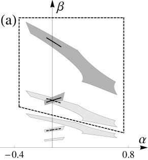
Figure 2: (a) The dark grey domain that consists of two connected components is the set $\mathfrak{R}$ of purely imaginary characteristic roots $i\beta$ of the interval polynomial (17) for Example 4.1. The two solid black curves inside the two components of $\mathfrak{R}$ show the set of purely imaginary roots for a representative polynomial $P(\alpha)(\cdot)$ that belongs to the family (17). This representative has two purely imaginary roots $i\beta_{1}(\alpha)$, $i\beta_{2}(\alpha)$ for some interval of $\alpha$ values $[\alpha_{1},\alpha_{2}]\subset(\alpha_{-},\alpha_{+})=(-0.4,0.8)$. The light grey domains are the sets $\mathfrak{S}_{2}$ and $\mathfrak{S}_{3}$ obtained from the dark grey domain $\mathfrak{R}$ by the transformations $(\alpha,\beta)\mapsto(\alpha,\beta/2)$ and $(\alpha,\beta)\mapsto(\alpha,\beta/3)$, respectively; the dashed curves inside $\mathfrak{S}_{2}$ are the images of the solid black curves in $\mathfrak{R}$ under this transformation. The intersection of the solid curve and the dashed curve inside the smaller component of $\mathfrak{R}$ corresponds to the $2:1$ resonance $i\beta_{1}(\alpha)=2i\beta_{2}(\alpha)$. The dashed quadrangle $\mathcal{D}_{1}$ contains the set $\mathfrak{R}$; its boundary does not intersect $\mathfrak{S}_{i}$ in accordance with (R5^′). (b) The real parts $\tau_{1}(\alpha)$, $\tau_{2}(\alpha)$ of the roots of the representative polynomial $P(\alpha,\cdot)$ that belongs to the family (17) (schematic). The sliding intervals $\tau_{1}(\alpha)=0$, $\tau_{2}(\alpha)=0$ correspond to the black curves $\beta_{1}(\alpha)$, $\beta_{2}(\alpha)$ shown inside the dark grey domain $\mathfrak{R}$ on panel (a).

Example 4.1 (Theorem 3.7 with (R5^′)).

Fix $\varepsilon=0.28$ and, for any real $\alpha$, define four intervals as follows:

$$J_{0}(\alpha) =\{4-4\alpha^{2}\};$$ (15)

$$J_{1}(\alpha) =[4\alpha-3\alpha^{2}+\alpha^{3}-\varepsilon,4\alpha-3\alpha^{2}+\alpha^{3}+\varepsilon];$$

$$J_{2}(\alpha) =[5-3\alpha+\alpha^{3}-\varepsilon,5-3\alpha+\alpha^{3}+\varepsilon];$$

$$J_{3}(\alpha) =\{\alpha+\alpha^{2}\}.$$

Consider the following forth order interval differential equation

$$J_{0}(\alpha)y+J_{1}(\alpha)y^{\prime}+J_{2}(\alpha)y^{\prime\prime}+J_{3}(\alpha)y^{\prime\prime\prime}+y^{\prime\prime\prime\prime}=\mathfrak{r}(\alpha,y,y^{\prime},y^{\prime\prime},y^{\prime\prime\prime}).$$ (16)

The characteristic equation of the linearization of (16) at zero has the form

$$\mathfrak{Q}(\alpha)(\lambda)=J_{0}(\alpha)+J_{1}(\alpha)\lambda+J_{2}(\alpha)\lambda^{2}+J_{3}(\alpha)\lambda^{3}+\lambda^{4}.$$ (17)

Following (14), we compute

$$\text{Im}(g_{1}(\mathfrak{Q}(\alpha),i\beta)) =4-4\alpha^{2}-(5-3\alpha+\alpha^{3}+\varepsilon)\beta^{2}+\beta^{4};$$

$$\text{Im}(g_{2}(\mathfrak{Q}(\alpha),i\beta)) =4-4\alpha^{2}-(5-3\alpha+\alpha^{3}-\varepsilon)\beta^{2}+\beta^{4};$$

$$\text{Re}(h_{1}(\mathfrak{Q}(\alpha),i\beta)) =(4\alpha-3\alpha^{2}+\alpha^{3}-\varepsilon)\beta-(\alpha+\alpha^{2})\beta^{3};$$

$$\text{Re}(h_{2}(\mathfrak{Q}(\alpha),i\beta)) =(4\alpha-3\alpha^{2}+\alpha^{3}+\varepsilon)\beta-(\alpha+\alpha^{2})\beta^{3}.$$

Take $\alpha_{-}=-0.4$ and $\alpha_{+}=0.8$ and define $\mathfrak{R}$ and $\mathfrak{S}$ as in (14). Let us show that equation (16) satisfies conditions of Theorem 3.7 with (R5^′). Since, by construction, $\alpha\in[-0.4,0.8]$, (R2) is satisfied (cf. the first formula in (15)). To show (R3) and (R4), we use Lemma 2.4. Observe that $\mathfrak{Q}(\alpha)(\lambda)$ from (17) is obtained from the polynomial $P_{o}(\alpha)(\lambda)=(\lambda^{2}+\alpha\lambda+1+\alpha)\cdot(\lambda^{2}+\alpha^{2}\lambda+4-4\alpha)$ by taking $\varepsilon$-neighborhoods of some of its coefficients. By direct verification, $P_{o}(\alpha_{+})$ is Hurwitz stable while $P_{o}(\alpha_{-})$ is $2$-unstable. To complete the verification of condition (R3) (resp., (R4)), it remains to observe that $\{(\alpha_{-},\beta)\in[\alpha_{-},\alpha_{+}]\times\mathbb{R}_{+}\}\cap\mathfrak{R}=\emptyset$ (resp., $\{(\alpha_{+},\beta)\in[\alpha_{-},\alpha_{+}]\times\mathbb{R}_{+}\}\cap\mathfrak{R}=\emptyset$). These last two relations as well as condition (R5^′) are illustrated by Figure 2.

Figure 3: (a) The nonintersecting sets $\mathfrak{R}$ (dark grey) and $\mathfrak{S}$ (light grey) for Example 4.2 with $[\alpha_{1},\alpha_{2}]=[-0.5,1.2]$. The black curve is the set of purely imaginary roots of a representative polynomial $P(\alpha)(\cdot)$ that belongs to the family (17). At the corner point of this curve, $P(\alpha)(\cdot)$ has a purely imaginary root of multiplicity 2. The real parts of the roots of $P(\alpha)(\cdot)$ behave as shown on panel (b) of Figure 2. (b) Curves $(w_{1}(\alpha_{\pm},\cdot),w_{2}(\alpha_{\pm},\cdot))$ (thick lines) for Example 4.3. The thin curve $(w_{1}(\alpha,\cdot),w_{2}(\alpha,\cdot))$ with $\alpha=0.075$ from the interior of the interval $[\alpha_{-},\alpha_{+}]$ intersects the negative cone $\{(w_{1},w_{2}):w_{1}\leq 0,\,w_{2}\leq 0\}$.

Example 4.2 (Theorem 3.7 with (R5^′′)).

Fix $\varepsilon=0.7$ and, for any real $\alpha$, define four intervals as follows:

$$J_{0}(\alpha) =[81+27\alpha+2\alpha^{2}-\varepsilon,81+27\alpha+2\alpha^{2}+\varepsilon];$$ (18)

$$J_{1}(\alpha) =[9\alpha+11\alpha^{2}+\alpha^{3}-\varepsilon,9\alpha+11\alpha^{2}+\alpha^{3}+\varepsilon];$$

$$J_{2}(\alpha) =\{18+3\alpha+\alpha^{3}\};$$

$$J_{3}(\alpha) =[\alpha+\alpha^{2}-\varepsilon,\alpha+\alpha^{2}+\varepsilon].$$

As in Example 4.1, consider the interval differential equation (16) and the characteristic polynomial of its linearization (17). In this case,

$$\text{Re}(g_{1}(\mathfrak{Q}(\alpha),i\beta)) =(81+27\alpha+2\alpha^{2}-\varepsilon)-(18+3\alpha+\alpha^{3})\beta^{2}+\beta^{4};$$

$$\text{Re}(g_{2}(\mathfrak{Q}(\alpha),i\beta)) =(81+27\alpha+2\alpha^{2}+\varepsilon)-(18+3\alpha+\alpha^{3})\beta^{2}+\beta^{4};$$

$$\text{Im}(h_{1}(\mathfrak{Q}(\alpha),i\beta)) =(9\alpha+11\alpha^{2}+\alpha^{3}-\varepsilon)\beta-(\alpha+\alpha^{2}+\varepsilon)\beta^{3};$$

$$\text{Im}(h_{2}(\mathfrak{Q}(\alpha),i\beta)) =(9\alpha+11\alpha^{2}+\alpha^{3}+\varepsilon)\beta-(\alpha+\alpha^{2}-\varepsilon)\beta^{3}.$$

Consider the interval $[\alpha_{-},\alpha_{+}]=[-0.5,1.2]$. For this interval, conditions (R2) – (R4) of Theorem 3.7 can be verified in the same way as in the previous example. In particular, one can use the representative polynomial $P_{o}(\alpha)(\lambda)=(9+\alpha+\alpha\lambda+\lambda^{2})(9+2\alpha+\alpha^{2}\lambda+\lambda^{2})$ when proving (R3) and (R4). Figure 3a shows that condition (R5^′′) is also satisfied.

Example 4.3 (Theorem 3.7 with (R5^′′′)).

Fix $\varepsilon=1$. For any real $\alpha$, define five intervals

$$J_{0}(\alpha) =[36-\varepsilon,36+\varepsilon];$$ (19)

$$J_{1}(\alpha) =[36+36\alpha-\varepsilon,36+36\alpha+\varepsilon];$$

$$J_{2}(\alpha) =[47+36\alpha-\varepsilon,47+36\alpha+\varepsilon];$$

$$J_{3}(\alpha) =[37+11\alpha-\varepsilon,37+11\alpha+\varepsilon];$$

$$J_{4}(\alpha) =[11+\alpha-\varepsilon,11+\alpha+\varepsilon]$$

and consider the fifth order interval differential equation

$$J_{0}(\alpha)y+J_{1}(\alpha)y^{\prime}+J_{2}(\alpha)y^{\prime\prime}+J_{3}(\alpha)y^{\prime\prime\prime}+J_{4}(\alpha)y^{\prime\prime\prime\prime}+y^{\prime\prime\prime\prime\prime}=\mathfrak{r}(\alpha,y,y^{\prime},y^{\prime\prime},y^{\prime\prime\prime},y^{\prime\prime\prime\prime}).$$ (20)

The corresponding characteristic polynomial equals

$$\mathfrak{Q}(\alpha)(\lambda)=J_{0}(\alpha)+J_{1}(\alpha)\lambda+J_{2}(\alpha)\lambda^{2}+J_{3}(\alpha)\lambda^{3}+J_{4}(\alpha)\lambda^{4}+\lambda^{5}.$$ (21)

Let us take $\alpha_{-}=-0.1$, $\alpha_{+}=0.09$ and show that conditions of Theorem 3.7 with (R5^′′′) are satisfied. By construction, $\varepsilon=1$, hence (R2) holds (cf. the first formula in (19)). To show (R5^′′′), we apply Lemma 2.6. To this end, put $Q(\lambda)=\lambda$ and $R(\lambda)=-5$. By direct calculation,

$$\mathcal{T}(\mathfrak{Q},Q,R)(\omega)=(-144-180\alpha\pm 6\varepsilon)\omega+(138+19\alpha\pm 6\varepsilon)\omega^{3}+(6+\alpha\pm\varepsilon)\omega^{5},$$

where for brevity we denote the interval $[\mu-\varepsilon,\mu+\varepsilon]$ by $\mu\pm\varepsilon$. Since for $\alpha\in[\alpha_{-},\alpha_{+}]$, $\mathcal{T}$ has at most one sign change, property (R5^′′′) is satisfied. Finally, to show (R3) and (R4), we use the same argument as in the previous examples observing that $\mathfrak{Q}$ in (21) is obtained from the polynomial $P_{o}(\alpha)(\lambda)=(2+\lambda)\cdot(3+\lambda)\cdot(6+\lambda)\cdot(1+\alpha\lambda+\lambda^{2})$ by taking $\varepsilon$-neighborhoods of some of its coefficients. By direct verification, $P_{o}(\alpha_{+})(\cdot)$ is Hurwitz stable while $P_{o}(\alpha_{-})(\cdot)$ is $2$-unstable. To complete the verification of condition (R3) (resp. (R4)), it remains to observe that the curves shown in Figure 3b don’t intersect the negative cone $\{(x,y)\in\mathbb{R}^{2}\;:\;x\leq 0,y\leq 0\}$ (cf. Lemma 2.4).

5 Proof of Theorem 3.2

5.1 Necessary condition for the Hopf bifurcation

Before proving Theorem 3.2, let us show that the assumptions of Theorem 3.2 imply the classical necessary condition for the Hopf bifurcation.

Proposition 5.1.

Under the assumptions of Theorem 3.2, there exists $(\alpha_{o},\beta_{o})\in\bigcup\mathcal{D}_{k}$ such that $\Lambda(\alpha_{o},\beta_{o},0)=0$.

Proof:    Observe (cf. property (P4)(i)) that $\partial\mathcal{P}$ is homeomorphic to a $2$-dimensional sphere. Take the standard orientation on $\mathbb{R}^{2}$ and induce an orientation on $\mathcal{P}_{0}\subset\partial\mathcal{P}$. This orientation canonically induces orientations on $\mathcal{P}_{\pm}$ and the orientation on $\partial\mathcal{P}$. In particular, the local Brouwer degree for $\Lambda|_{\partial\mathcal{P}}:\partial\mathcal{P}\to\mathbb{C}$ is correctly defined (provided that, say, the standard orientaion on $\mathbb{C}\simeq\mathbb{R}^{2}$ is chosen). Since $\partial\mathcal{P}$ is compact and $\mathbb{C}$ is not compact, it follows that $\Lambda|_{\partial\mathcal{P}}$ is not surjective and, therefore,

$$\deg(\Lambda,\partial\mathcal{P})=0$$ (22)

(cf. [17], Chapter VIII, Subsection 4.5). Combining (22) with condition (P4)(ii) and the excision property of the local Brouwer degree, one has (cf. [5], p. 277):

$$\deg(\Lambda,\partial\mathcal{P})=\deg(\Lambda,\mathcal{P}_{+})+\deg(\Lambda,\mathcal{P}_{-})+\deg(\Lambda,\mathcal{P}_{0})=0.$$ (23)

By construction, the orientation on $\mathcal{P}_{+}$ (resp., $\mathcal{P}_{-}$) coincides with the orientation on $\mathcal{P}_{0}$ (resp., is opposite to it). Denote by $\mathfrak{t}_{\pm}$ the number of roots of $\Lambda(\alpha_{\pm},\beta,\tau)$ in $\mathcal{P}_{\pm}$ (counted according to their multiplicities). It is easy to see that $\mathfrak{t}_{\pm}=\pm\deg(\Lambda,\mathcal{P}_{\pm})$. This observation together with formula (23) implies

$$\deg(\Lambda,\mathcal{P}_{0})=\mathfrak{t}_{-}-\mathfrak{t}_{+}\not=0$$

(cf. condition (P4(iii)). On then other hand, combining condition (P5)(ii) with the $\mathbb{Z}_{2}$-equivariance of $\Lambda$ (see condition (P4)) yields

$${\mathfrak{t}_{-}-\mathfrak{t}_{+}\over 2}={1\over 2}\deg(\Lambda,\mathcal{P}_{0})=\deg(\Lambda,\bigcup\mathcal{D}_{k}).$$ (24)

By the existence property of the Brouwer degree, the conclusion follows. $\square$

5.2 Normalization of the period

We are looking for periodic solutions, with unknown period $p$, of the differential equation

$$\dot{x}=f(\alpha,x).$$

Following the standard scheme, let us introduce the unknown period $p$ as an additional parameter. Define $\beta=\frac{2\pi}{p}$ and apply the change of variables

$$u(t)=x\Big{(}\frac{pt}{2\pi}\Big{)}$$

to obtain the system

$$\begin{cases}\dot{u}=\frac{1}{\beta}f(\alpha,u),\\ u(0)=u(2\pi).\end{cases}$$ (25)

We are now in a position to reformulate the original problem as an operator equation in the appropriate space of $2\pi$-periodic functions and apply the equivariant degree method.

5.3 $S^{1}$-representations

We will use the first Sobolev space of functions on the unit circle equipped with the natural structure of $S^{1}$-representation induced by the shift in time. Let us recall some standard facts related to $S^{1}$-representations. As is well-known (see, for example, [12]), any real irreducible $S^{1}$-representation is of dimension $1$ or $2$ and can be described as follows. Take an integer $l>0$ and define the $S^{1}$-action on $\mathbb{C}\simeq\mathbb{R}^{2}$ by $(e^{i\varphi},z)\mapsto e^{il\varphi}\cdot z$, where “$\cdot$” stands for complex multiplication,(denote this representation $\mathcal{V}_{l}$); also, denote by $\mathcal{V}_{0}$ the trivial one-dimensional $S^{1}$-representation.

Define $V=\mathbb{R}^{n}$. Denote by $W=H^{1}(S^{1};V)$ the first Sobolev space of functions from $S^{1}$ to $V$. Observe that $W$ admits the “Fourier decomposition”

$$W=\overline{V\oplus\bigoplus^{\infty}_{l=1}W_{l}},$$ (26)

where the subspace of zero Fourier modes (i.e., constant functions) is identified with $V$, while the subspace of the $l$-th Fourier modes $W_{l}$ is identified with the complexification of $V$ (denoted $V^{c}$). In particular, any function $u\in W_{l}$ can be written in the form $e^{ilt}\cdot(x_{l}+iy_{l})$ for some $x_{l},y_{l}\in V$. There is a natural orthogonal $S^{1}$-representation on $W$ given by

$$(e^{i\varphi},u)(t)\mapsto u(t+\varphi),\quad e^{i\varphi}\in S^{1},\;u\in W.$$ (27)

Formula (27) gives rise to the trivial action on $V$ and the action $(e^{i\varphi},u)(t)\mapsto e^{il\varphi}\cdot u(t)$ on $W_{l}$.

5.4 Reformulation in the functional space

Take the first Sobolev space $W$ and define the orthogonal projector $K:W\to L^{2}(S^{1};V)$ by

$$K(u)={1\over 2\pi}\int_{0}^{2\pi}u(t)dt,\quad u\in W.$$ (28)

We can now rewrite (25) as the following operator equation in $[\alpha_{-},\alpha_{+}]\times\mathbb{R}_{+}\times W$:

$$\mathfrak{F}(\alpha,\beta,u)=u-\mathcal{F}(\alpha,\beta,u)=0,\quad(\alpha,\beta)\in[\alpha_{-},\alpha_{+}]\times\mathbb{R}_{+},\;\;u\in W,$$ (29)

where

$$\mathcal{F}(\alpha,\beta,u)=(L+K)^{-1}\Big{(}{1\over\beta}F(\alpha,u)+Ku\Big{)},$$ (30)

$L:W\to L^{2}(S^{1};V)$ is given by $L(x)=\dot{x}$ and $F:\mathbb{R}\times W\to L^{2}(S^{1};V)$ is defined by $F(\alpha,u)(t)=f(\alpha,u(t))$. Formula (27) gives rise to the $S^{1}$-action on $[\alpha_{-},\alpha_{+}]\times\mathbb{R}_{+}\times W$ (we assume that $S^{1}$ acts trivially on $[\alpha_{-},\alpha_{+}]\times\mathbb{R}_{+}$). Moreover, it is easy to see that $\mathfrak{F}$ given by (29) and (30) is $S^{1}$-equivariant.

5.5 Reducing the problem to computing $S^{1}$-degree

In order to apply the equivariant degree method, we need to localize potential bifurcating branches in a cylindric box $\Omega\subset[\alpha_{-},\alpha_{+}]\times\mathbb{R}_{+}\times W$ in such a way that the operator (29) is $\Omega$-admissible. To this end, consider the sets $\mathcal{D}_{k}$ provided by condition (P5) and put $\Sigma_{k}=\partial\mathcal{D}_{k}$. Since $\Sigma_{k}$ is compact, there are disjoint neighborhoods $N_{k}$ of $\Sigma_{k}\subset[\alpha_{-},\alpha_{+}]\times\mathbb{R}_{+}$ such that $\Lambda(\alpha,\beta,0)\neq 0$ for all $(\alpha,\beta)\in\overline{N_{k}}$. Set

$$\widetilde{\mathcal{D}}_{k}=\mathcal{D}_{k}\cup N_{k};\quad\widetilde{\Sigma}_{k}=\partial\widetilde{\mathcal{D}}_{k};\quad\widetilde{\mathcal{D}}=\bigcup\widetilde{\mathcal{D}}_{k};\quad\quad\widetilde{\Sigma}=\partial\widetilde{\mathcal{D}};\quad a(\alpha,\beta)={\rm Id}-D_{u}\mathcal{F}(\alpha,\beta,0),$$ (31)

where $D_{u}\mathcal{F}$ denotes the derivative of $\mathcal{F}$ with respect to $u$ (cf. (30)).

Lemma 5.2.

There exists a disc $B_{r}(0)\subset W$ of radius $r$ centered at the origin such that for all points $(\alpha,\beta,u)\in\widetilde{\Sigma}\times(B_{r}(0)\setminus\{0\})$, the following holds:

(i) $u-\mathcal{F}(\alpha,\beta,u)\neq 0$;

(ii) the fields $\mathfrak{F}(\alpha,\beta,\cdot)$ and $a(\alpha,\beta)$ are $S^{1}$-equivariantly homotopic on $B_{r}(0)$.

Proof:

(i) For a contradiction, suppose that for all $\rho>0$, there exists $(\alpha,\beta,u)\in\widetilde{\Sigma}\times(B_{\rho}\setminus\{0\})$ with $u-\mathcal{F}(\alpha,\beta,u)=0$. Since $\widetilde{\Sigma}$ is compact, without loss of generality, assume that there exists a sequence $(\alpha_{j},\beta_{j},u_{j})$ converging to $(\alpha_{*},\beta_{*},0)$ such that $(\alpha_{j},\beta_{j})\in\widetilde{\Sigma}$, $u_{j}-\mathcal{F}(\alpha_{j},\beta_{j},u_{j})=0$ and $u_{j}\not=0$. Then,

$$\frac{u_{j}}{\|u_{j}\|}-\frac{\mathcal{F}(\alpha_{j},\beta_{j},u_{j})}{\|u_{j}\|}=0.$$

Observe that $(\alpha_{j},\beta_{j})\in\widetilde{\Sigma}$ implies that $\beta_{j}$ does not converge to $0$. Combinig this with assumption (P1) and (30) yields

$$\frac{u_{j}}{\|u_{j}\|}-D_{u}\mathcal{F}(\alpha_{j},\beta_{j},0)\frac{u_{j}}{\|u_{j}\|}+\frac{r(\alpha_{j},\beta_{j},u_{j})}{\|u_{j}\|}=0,$$ (32)

where $r(\alpha_{j},\beta_{j},u_{j})=\mathcal{F}(\alpha_{j},\beta_{j},u_{j})-D_{u}\mathcal{F}(\alpha_{j},\beta_{j},0)u$. Also,

$$D_{u}\mathcal{F}(\alpha_{j},\beta_{j},0)\frac{u_{j}}{\|u_{j}\|}=D_{u}\mathcal{F}(\alpha_{*},\beta_{*},0)\frac{u_{j}}{\|u_{j}\|}+(D_{u}\mathcal{F}(\alpha_{j},\beta_{j},0)-D_{u}\mathcal{F}(\alpha_{*},\beta_{*},0)){u_{j}}/{\|u_{j}\|}.$$ (33)

Since $D_{u}\mathcal{F}(\alpha_{*},\beta_{*},0)$ is compact, without loss of generality, we can assume that $D_{u}\mathcal{F}(\alpha_{*},\beta_{*},0){u_{j}}/{\|u_{j}\|}$ converges to some $v_{*}$. In addition, keeping in mind that $D_{u}\mathcal{F}(\alpha_{*},\beta_{*},0)$ depends continuously on $\alpha,\beta$, it follows from (33) that $D_{u}\mathcal{F}(\alpha_{j},\beta_{j},0){u_{j}}/{\|u_{j}\|}$ converges to $v_{*}$. Combining this with (7) and (32) yields that ${u_{j}}/{\|u_{j}\|}$ converges to $v_{*}\neq 0$. Hence (see (32) once again),

$$v_{*}-D_{u}\mathcal{F}(\alpha_{*},\beta_{*},0)v_{*}=0$$

meaning that $\text{Id}-D_{u}\mathcal{F}(\alpha_{*},\beta_{*},0)$ is not invertible, which contradicts (P5)(iii).

(ii) This part trivially follows from the compactness of $\widetilde{\Sigma}$ and condition (P5)(iii) combined with the standard linearization argument. $\square$

Take $\widetilde{\mathcal{D}}_{k}$ given by (31) and $B_{r}(0)$ provided by Lemma 5.2. Define

$$\Omega_{k}=\{\left(\alpha,\beta,u\right)\in[\alpha_{-},\alpha_{+}]\times\mathbb{R}_{+}\times W:(\alpha,\beta)\in\widetilde{\mathcal{D}}_{k},\;u\in B_{r}(0)\},\qquad\Omega=\bigcup\Omega_{k}.$$ (34)

Clearly, $\Omega$ is $S^{1}$-invariant. By the existence of the invariant Urysohn function, one can take an invariant function $\varsigma:\Omega\to\mathbb{R}$ satisfying the properties

$$\varsigma(\alpha,\beta,0)<0;\qquad\varsigma(\alpha,\beta,u)>0\quad\text{for}\quad\|u\|=r.$$ (35)

Consider the map $\mathfrak{F}_{\varsigma}:\Omega\to\mathbb{R}\oplus W$ given by

$$\mathfrak{F}_{\varsigma}(\alpha,\beta,u)=(\varsigma(\alpha,\beta,u),\mathfrak{F}(\alpha,\beta,u)).$$ (36)

By definition, any solution to the equation $\mathfrak{F}_{\varsigma}(\alpha,\beta,u)=0$ is also a solution to (25). In addition, $\mathfrak{F}_{\varsigma}$ is an $S^{1}$-equivariant $\Omega$-admissible map for which $S^{1}\text{-Deg\,}(\mathfrak{F}_{\varsigma},\Omega)$ is correctly defined.

Remark 5.3.

As long as an invariant Urysohn function $\varsigma$ satisfies properties (35), $S^{1}\text{-Deg\,}(\mathfrak{F}_{\varsigma},\Omega)$ is independent of the choice of $\varsigma$ (homotopy property of the $S^{1}$-degree).

The next statement provides a sufficient condition for the existence of a branch of periodic solutions bifurcating from the trivial solution (cf. Definition 2.1). We follow the scheme suggested in [5] (see Theorem 9.18) with several modifications making the argument more transparent.

Proposition 5.4.

Given system (1), assume conditions (P0) – (P5) are satisfied. Take $\Omega$ defined by (34) and $\mathfrak{F}_{\varsigma}$ defined by (36). Assume $S^{1}\text{\rm-Deg\,}(\mathfrak{F}_{\varsigma},\Omega)\not=0$. Then, system (1) has a branch of periodic solutions bifurcating from the trivial solution.

As in [5], the following statement is the main topological ingredient in the proof of Proposition 5.4 (cf. Theorem 3 in [37], p. 170).

Proposition 5.5 (Kuratowski).

Let $X$ be a metric space, $A,B\subset X$ two disjoint closed sets in $X$, and $K$ a compact set in $X$ such that $K\cap A\not=\emptyset\not=K\cap B$. If the set $K$ does not contain a connected component $K_{o}$ such that $K_{o}\cap A\not=\emptyset\not=K_{o}\cap B$, then there exist two disjoint open sets $V_{1}$, $V_{2}$ such that $A\subset V_{1}$, $B\subset V_{2}$ and $A\cup B\cup K\subset V_{1}\cup V_{2}$.

Proof of Proposition 5.4. Put

$$K=\mathfrak{F}^{-1}(0)\cap\overline{\Omega}.$$

Consider the family of invariant functions $\varsigma_{q}:\overline{\Omega}\to\mathbb{R}$ given by

$$\varsigma_{q}(\alpha,\beta,u)=\|u\|-q,\;\quad 0\leq q\leq r.$$

Suppose for contradiction, there does not exist a compact connected set $K_{o}\subset K$ with $K_{o}\cap\varsigma_{0}^{-1}(0)\not=\emptyset\not=K_{o}\cap\varsigma_{r}^{-1}(0)$. To apply Proposition 5.5, we need to show that $K\cap\varsigma_{0}^{-1}(0)\not=\emptyset\not=K\cap\varsigma_{r}^{-1}(0)$. Notice that for any $q\in(0,r)$, $\varsigma_{q}$ satisfies properties (35), so $S^{1}\text{-Deg\,}(\mathfrak{F}_{\varsigma_{q}},\Omega\neq 0$ (cf Remark 5.3 and the assumptions of Proposition 5.4. By the existence property of $S^{1}$-degree, for each $q\in(0,r)$ there exists $(\alpha_{q},\beta_{q},u_{q})\in K$ with $\|u_{q}\|=q.$ Since K is compact, it follows that there exist $(\alpha_{0},\beta_{0},u_{0})\in K\cap\varsigma_{0}^{-1}(0)$ and $(\alpha_{r},\beta_{r},u_{r})\in K\cap\varsigma_{r}^{-1}(0)$.

Put

$$A^{\prime}=\{(\alpha,\beta,u)\in\overline{\Omega}\;:\;\|u\|=0\},\quad A^{\prime\prime}=\{(\alpha,\beta,u)\in\overline{\Omega}\;:\;\|u\|=r\}.$$

Then, by Proposition 5.5, there exist open disjoint sets $N^{\prime}\supset A^{\prime}$, $N^{\prime\prime}\supset A^{\prime\prime}$ with $K\subset N^{\prime}\cup N^{\prime\prime}$. Put

$$Z^{\prime}=\overline{A^{\prime}\cup(K\cap N^{\prime})};\quad Z^{\prime\prime}=\overline{A^{\prime\prime}\cup(K\cap N^{\prime})}$$ (37)

and let us, first, show that $Z^{\prime}$ is $S^{1}$-invariant. Notice that $A^{\prime}$ is invariant. Suppose for contradiction that $K\cap N^{\prime}$ is not invariant. Then, there exist $u\in K\cap N^{\prime}$ and $\gamma\in S^{1}$ such that $(\gamma,u)\notin K\cap N^{\prime}$. However, since $K$ is invariant and $K\subset N^{\prime}\cup N^{\prime\prime}$, it follows that $(\gamma,u)\in K\cap N^{\prime\prime}$. We now have $S^{1}(u)\subset N^{\prime}\cup N^{\prime\prime}$ with $S^{1}(u)\cap N^{\prime}\not=\emptyset\not=S^{1}(u)\cap N^{\prime\prime}$ and $N^{\prime}\cap N^{\prime\prime}=\emptyset$, which contradicts the connectedness of $S^{1}(u)$. Thus, $Z^{\prime}$ is invariant as the union of invariant sets. Similarly, $Z^{\prime\prime}$ is also invariant.

Next, define an invariant Urysohn function $\mu:\overline{\Omega}\to\mathbb{R}$ with the following property:

$$\mu(\alpha,\beta,u)=\begin{cases}1,\quad{\rm if}\;(\alpha,\beta,u)\in Z^{\prime};\\ 0,\quad{\rm if}\;(\alpha,\beta,u)\in Z^{\prime\prime}.\end{cases}$$ (38)

Take $\varsigma:\overline{\Omega}\to\mathbb{R}$ defined by

$$\varsigma(\alpha,\beta,u)=\|u\|-\mu(\alpha,\beta,u)\cdot r.$$ (39)

Clearly, $\varsigma$ is invariant and satisfies properties (35) (cf Remark 5.3 and the assumptions of Proposition 5.4) so $S^{1}\text{-Deg\,}(\mathfrak{F}_{\varsigma},\Omega)\neq 0$. By the existence property of the $S^{1}$-degree, there exists $(\alpha_{\ast},\beta_{\ast},u_{\ast})$ with $\|u\|-\mu(\alpha_{\ast},\beta_{\ast},u_{\ast})=0$. Since $K\subset N^{\prime}\cup N^{\prime\prime}$ and $N^{\prime}\cap N^{\prime\prime}=\emptyset$, it follows that either $(\alpha_{\ast},\beta_{\ast},u_{\ast}))\in N^{\prime}$ or $(\alpha_{\ast},\beta_{\ast},u_{\ast})\in N^{\prime\prime}$. Assume $(\alpha_{\ast},\beta_{\ast},u_{\ast})\in N^{\prime}$. Then (cf. (37), (38)) and (39)), $\|u_{\ast}\|=r$, i.e. $(\alpha_{\ast},\beta_{\ast},u_{\ast})\in A^{\prime\prime}\cap N^{\prime}=\emptyset$. Similarly, the assumption $(\alpha_{\ast},\beta_{\ast},u_{\ast})\in N^{\prime\prime}$ leads to a contradiction.

5.6 Computation of $S^{1}\text{-Deg\,}(\mathfrak{F}_{\varsigma},\Omega)$ via deformations

Proposition 5.4 reduces the proof of Theorem 3.2 to the computation of $S^{1}\text{\rm-Deg\,}(\mathfrak{F}_{\varsigma},\Omega)$ and showing that this degree is non-zero. Our goal now is to connect $S^{1}\text{\rm-Deg\,}(\mathfrak{F}_{\varsigma},\Omega)$ to spectral properties of $D_{x}f(\alpha,0)$ (cf. condition (P1)). This will be done in several steps.

Step I: Reduction to a circle. Put $\widetilde{\mathfrak{F}}_{\varsigma}(\alpha,\beta,u)=(\varsigma(\alpha,\beta,u),a(\alpha,\beta)u)$ (cf. (31)). Since $\varsigma(\alpha,\beta,0)<0$, it follows from Lemma 5.2(ii) that $\widetilde{\mathfrak{F}}_{\varsigma}$ is $S^{1}$-equivariantly homotopic to $\mathfrak{F}_{\varsigma}$ on $\Omega_{k}$.

Take $\widetilde{D}_{k}$ and $N_{k}$ from (31) and assume, without loss of generality, that $N_{k}$ is homeomorphic to $[-1,1]\times S^{1}$. Let $(\xi_{k},\gamma_{k}):N_{k}\to[-1,1]\times S^{1}$ be a trivialization taking $\widetilde{\Sigma}_{k}$ to $\{1\}\times S^{1}$. For any $k$, define three functions $g_{k}:\widetilde{\mathcal{D}}_{k}\to\mathbb{R}$, $\widetilde{\varsigma}_{k}:\Omega_{k}\to\mathbb{R}$ and $\widetilde{}\mathfrak{F}_{1k}:\Omega_{k}\to\mathbb{R}\oplus W$ by

$$g_{k}(\alpha,\beta)=\begin{cases}0,&(\alpha,\beta)\in\widetilde{\mathcal{D}}_{k}\setminus N_{k};\\ \xi_{k}(\alpha,\beta)+1,&(\alpha,\beta)\in N_{k};\end{cases}$$ (40)

$$\widetilde{\varsigma}_{k}(\alpha,\beta,u)=g_{k}(\alpha,\beta)(\|u\|-r)+\|u\|+r;$$ (41)

$$\mathfrak{F}_{k}^{1}(\alpha,\beta,u)=(\widetilde{\varsigma}_{k}(\alpha,\beta,u),a(\alpha,\beta)u).$$ (42)

Obviously, the boundary $\partial\Omega_{k}$ of the domain $\Omega_{k}$ consists of three pieces:

$$\partial\Omega_{k}=\{\|u\|=r\}\;\cup\;\{u=0,\,\xi_{k}(\alpha,\beta)=1\}\;\cup\;\{u\neq 0,\ \xi_{k}(\alpha,\beta)=1\}.$$

On the first piece, $\varsigma_{k}$ and $\widetilde{\varsigma}_{k}$ are both positive, while on the second piece they are both negative. Also, on the third piece $a(\alpha,\beta)u$ is non-zero. Hence, the vector fields $\mathfrak{F}_{k}^{1}$ and $\widetilde{\mathfrak{F}}_{\varsigma}$ are not directed oppositely on $\partial\Omega_{k}$, therefore they are equivariantly homotopic on $\overline{\Omega}_{k}$. Define $\Omega_{k}^{1}=N_{k}\times B_{r}(0)$. By (40) and (41), for all $(\alpha,\beta)\in\widetilde{\mathcal{D}}_{k}\setminus N_{k}$, one has $\widetilde{\varsigma}_{k}>0$. Hence, by the excision and homotopy properties of the $S^{1}$-degree (see Appendix), $S^{1}\text{-Deg\,}(\mathfrak{F}_{\varsigma},\Omega_{k})=S^{1}\text{-Deg\,}(\mathfrak{F}_{k}^{1},\Omega_{k}^{1})$.

Define $\eta_{k}:N_{k}\to\Sigma_{k}$ by $\eta_{k}(\alpha,\beta)=(\xi_{k},\gamma_{k})^{-1}(0,\gamma_{k}(\alpha,\beta))$ and $\tilde{\mathfrak{F}}_{k}:\Omega_{k}^{1}\to\mathbb{R}\oplus W$ by

$$\widetilde{\mathfrak{F}}_{k}(\alpha,\beta,u)=(\widetilde{\varsigma}_{k}(\alpha,\beta,u),a(\eta_{k}(\alpha,\beta))u).$$ (43)

Then, by the homotopy property of the $S^{1}$-degree,

$$S^{1}\text{-Deg\,}(\mathfrak{F}_{\varsigma},\Omega_{k})=S^{1}\text{-Deg\,}(\widetilde{\mathfrak{F}}_{k},\Omega_{k}^{1}).$$ (44)

Observe that formulas (43), (44) reduce the computation of $S^{1}\text{-Deg\,}(\mathfrak{F}_{\varsigma},\Omega_{k})$ to studying $S^{1}$-equivariant homotopy properties of restrictions of $a_{k}:N_{k}\to GL^{S^{1}}_{c}(W)$ to the zero section $\Sigma_{k}\simeq\{0\}\times S^{1}$, where $GL^{S^{1}}_{c}(W)$ stands for the group of $S^{1}$-equivariant linear completely continuous vector fields in $W$.

Step II: Computation of the degree. For any $m\in\mathbb{N}$, put $W^{m}=V\oplus W_{1}\oplus...\oplus W_{m}$ (cf. (26)). Combining the compactness of the operator $a$ with the suspension property of the $S^{1}$-equivariant degree (see Appendix), one can find a sufficiently large $m$ such that the field $\widetilde{\mathfrak{F}}_{k}$ is equivariantly homotopic to the compact field $\mathfrak{F}_{k}^{2}:\overline{\Omega}_{k}^{1}\to\mathbb{R}\oplus W$ defined by

$$\mathfrak{F}_{k}^{2}(\alpha,\beta,u)=(\widetilde{\varsigma}_{k}(\alpha,\beta,u),\widetilde{a}(\eta_{k}(\alpha,\beta))u),$$ (45)

where $\widetilde{a}_{k}(\alpha,\beta)=a_{k}(\alpha,\beta)|_{W^{m}}+{\rm Id}|_{(W^{m})^{\perp}}$. Put

$$\widetilde{a}_{k}^{0}(\alpha,\beta):=\widetilde{a}_{k}(\alpha,\beta)|_{V};\quad\widetilde{a}_{k}^{l}(\alpha,\beta):=\widetilde{a}_{k}(\alpha,\beta)|_{W_{l}},\;l>0.$$ (46)

Fix some $\overline{\alpha}$ between $\alpha_{-}$ and $\alpha_{+}$. By condition (P3), the map $\widetilde{a}_{k}^{0}:N_{k}\to GL(V)$ is homotopic to the constant map $\overline{a}:N_{k}\to GL(V)$ given by $\overline{a}(\alpha,\beta)\equiv-D_{x}f(\overline{\alpha},0)$. Now, we are going to use formula (55) presented in Appendix. To this end, one needs to separate the “contribution” of the zero Fourier mode to the $S^{1}$-degree from other modes. Define

$$\Omega_{k}^{2}=\Omega_{k}^{1}\cap\big{(}\mathbb{R}^{2}\oplus W^{m}),\quad\Omega_{k}^{\ast}=B\times\Omega_{k}^{2},$$ (47)

where $B$ is the unit ball in $V$. Also, define $\hat{\mathfrak{F}}_{k}:\overline{\Omega_{k}^{2}}\to\mathbb{R}\oplus W$ and $\mathfrak{F}^{\ast}_{k}:\overline{\Omega_{k}^{\ast}}\to V\oplus\big{(}\mathbb{R}\oplus W\big{)}$ by

$$\hat{\mathfrak{F}}_{k}(\alpha,\beta,u)=(\widetilde{\varsigma}_{k}(\alpha,\beta,u),\bigoplus_{l=1}^{m}\widetilde{a}_{k}^{l}(\eta_{k}(\alpha,\beta))u),\quad\mathfrak{F}^{\ast}_{k}=\overline{a}\times\hat{\mathfrak{F}}_{k}.$$ (48)

Combining the suspension property of the $S^{1}$-degree with the product formula (see [5], Theorem 6.8), one obtains

$$S^{1}\text{-Deg\,}(\mathfrak{F}_{\varsigma},\Omega_{k})=S^{1}\text{-Deg\,}(\mathfrak{F}^{\ast}_{k},\Omega_{k}^{\ast})=\text{\rm sign\,}(\det(\overline{a}))\cdot S^{1}\text{-Deg\,}(\hat{\mathfrak{F}}_{k},\Omega_{k}^{2}).$$ (49)

Further, by applying formula (55),

$$S^{1}\text{-Deg\,}(\mathfrak{F}_{\varsigma},\Omega_{k})=\text{\rm sign\,}(\det(\overline{a}))\cdot\sum_{l=1}^{m}\big{(}\deg(\text{det}_{\mathbb{C}}(\widetilde{a}_{k}^{l}),\widetilde{}\mathcal{D}_{k})(\mathbb{Z}_{l})\big{)}.$$ (50)

Finally, applying the additivity property of $S^{1}\text{-Deg\,}$ and the Brouwer degree, we get

$$S^{1}\text{-Deg\,}(\mathfrak{F}_{\varsigma},\Omega) =\text{\rm sign\,}(\det(\overline{a}))\cdot\sum_{k}\sum_{l=1}^{m}\big{(}\deg(\text{det}_{\mathbb{C}}(\widetilde{a}_{k}^{l}),\widetilde{}\mathcal{D}_{k})(\mathbb{Z}_{l})\big{)}$$ (51)

$$=\text{\rm sign\,}(\det(\overline{a}))\cdot\sum_{l=1}^{m}\big{(}\deg(\text{det}_{\mathbb{C}}(a_{l}),\widetilde{}\mathcal{D})(\mathbb{Z}_{l})\big{)},$$

where $a_{l}(\alpha,\beta)=a(\alpha,\beta)|_{W_{l}}$.

Step III: Reduction to crossing numbers. Observe (see [5, p. 266]) that

$$a_{l}(\alpha,\beta)=\frac{1}{il\beta}[il\beta\,{\text{\rm Id}}-D_{x}f(\alpha,0)].$$

Put $a^{\prime}_{l}(\alpha,\beta)=il\beta\cdot a_{l}(\alpha,\beta)$. Since $\beta>0$, the map $a^{\prime}_{l}$ is homotopic to $a_{l}$. Note (cf. (8)) that $\text{det}_{\mathbb{C}}(a^{\prime}_{1}(\alpha,\beta))=\Lambda(\alpha,\beta,0)$. Finally (cf. condition (P4)(iii) and (24)),

$$\deg(\text{det}_{\mathbb{C}}(a_{1}),\widetilde{}\mathcal{D})=\frac{\mathfrak{t}_{-}-\mathfrak{t}_{+}}{2}\not=0.$$

Hence (cf. (51)), $S^{1}\text{-Deg\,}(\mathfrak{F}_{\varsigma},\Omega)\neq 0$. The application of Proposition 5.4 completes the proof.

6 Proof of Theorems 3.5 and 3.7

6.1 Proof of Theorem 3.5(a,b,c)

(a) Our goal is to construct a domain $\mathcal{P}$ satisfying (P4) in such a way that (P5^′) would imply (P5). To this end, take $\mathcal{D}_{k}$ provided by (P5^′) and $\alpha_{-}$, $\alpha_{+}$ provided by (P4^′). Next, take a sufficiently large $M>0$ to ensure that

$$\Lambda^{-1}(0)\subset\{[\alpha_{-},\alpha_{+}]\times B_{M}(0)\}=:B,$$ (52)

where $B_{M}(0)$ stands for the closed ball of radius $M$ centered at the origin in the $(\beta,\tau)$-plane. Also due to compactness, there exists a $\delta>0$ such that

$$\Lambda^{-1}(0)\cap\{0\leq\tau\leq\delta\}\subset{\rm int}(\bigcup\mathcal{D}_{k})\times\{0\leq\tau\leq\delta\}.$$ (53)

Define

$$\mathcal{P}=\Big{(}B\cap\{\tau\geq\delta\}\Big{)}\cup\bigcup\mathcal{D}_{k}\times\{0\leq\tau\leq\delta\}.$$ (54)

Since $B\cap\mathcal{D}_{k}\times\{0\leq\tau\leq\delta\}$ is homeomorphic to a disc, $\mathcal{P}$ satisfies (P4)(i). By the choice of $M$ and $\delta$ (see (52) and (53)), $\mathcal{P}$ satisfies (P4)(ii). Also, (P4)^′ guarantees (P4)(iii). Finally, by construction, $\mathcal{P}$ and $\mathcal{D}_{k}$ satisfy (P5)(ii).

(b) To prove Part (b), it suffices to deduce (P5^′) from (P5^′′). Notice that $R(f)$ is the set of roots of polynomials with coefficients parameterized by $\alpha\in[\alpha_{-},\alpha_{+}]$. Hence, the coefficients of these polynomials are uniformly bounded. Observe also that the leading coefficient of these polynomials is identically equal to $1$, therefore $R(f)$ is a compact set.

For any $\varepsilon>0$, there exists a sufficiently large $m$ such that $\bigcup^{\infty}_{k=m}S_{i}(f)\subset[\alpha_{-},\alpha_{+}]\times\{\beta<\varepsilon\}$. Since $[\alpha_{-},\alpha_{+}]$ is compact and $D_{x}f(\cdot,0)$ is non-singular, it follows that $R(f)$ is uniformly separated from $[\alpha_{-},\alpha_{+}]\times\{\beta<\varepsilon\}$ provided that $\varepsilon$ is small enough. On the other hand, the sets $\bigcup^{m-1}_{k=2}S_{i}(f)$ and $R(f)$ are compact and disjoint (see condition (P5^′′)), so they can be uniformly separated. Hence there exists a neighborhood $N_{\varepsilon}(R(f))$ of $R(f)$ in $[\alpha_{-},\alpha_{+}]\times\mathbb{R}_{+}$ such that $N_{\varepsilon}(R(f))\cap S(f)=\emptyset$. Without loss of generality, one can assume that $N_{\varepsilon}(R(f))$ is a finite union of discs, therefore, the complement to $N_{\varepsilon}(R(f))$ in $[\alpha_{-},\alpha_{+}]\times\mathbb{R}_{+}$ has finitely many bounded connected components, say, $\{U_{i}\}_{i=1}^{K}$. Set

$$\mathcal{D}=N_{\varepsilon}(R(f))\cup\bigcup_{i=1}^{K}U_{i}.$$

By construction, $\overline{\mathcal{D}}$ is a finite collection of disjoint sets homeomorphic to closed discs (denoted $\mathcal{D}_{k}$) and $\partial\mathcal{D}_{k}\subset\partial N_{\varepsilon}(R(f))$, thus $\mathcal{D}_{k}$ satisfies condition (P5^′). Hence, the result follows from Theorem 3.5(a).

(c) To prove part (c), it suffices to deduce (P5^′′) from (P5^′′′). To this end, assume, by contradiction, that (P5^′′) is not satisfied. Then, there exist a point $(\alpha,\beta)\in[\alpha_{-},\alpha_{+}]\times\mathbb{R}_{+}$ and an integer $k\geq 2$ such that $(\alpha,\beta),(\alpha,k\beta)\in R(f)$. This contradicts (P5^′′′).

6.2 Proof of Theorem 3.5(d)

Let $\mathcal{P}$ be the set provided by condition (P4). Our first goal is to construct $\mathcal{P}^{\prime}\supset\mathcal{P}$ such that (a) $\mathcal{P}^{\prime}$ satisfies (P4); and, (b) $\mathcal{P}^{\prime}_{0}$ is a disjoint union of finitely many sets homeomorphic to a closed disc (cf. (9)). To this end, without loss of generality (use a small perturbation of $\mathcal{P}$ if necessary), one can assume that $\mathcal{P}_{0}\subset[\alpha_{-},\alpha_{+}]\times\mathbb{R}_{+}$ is a disjoint union $\cup_{i=1}^{m}K_{i}$, where $K_{i}$ is a $(\nu_{i}+1)$-connected compact domain. Using the same surgery argument as in the proof of Alexander’s tame sphere Theorem (see, for example, [11], Theorem 4.34), one can construct $\mathcal{P}^{\prime}$ satisfying (a) and (b).

Our next goal is to construct a finite collection of discs $\mathcal{D}_{k}\subset[\alpha_{-},\alpha_{+}]\times\mathbb{R}_{+}$ satisfying (P5). Take $R$ and $S$ given by (10). Using the same argument as in the proof of Theorem 3.5(b) above, one can construct a sufficiently small neighborhood $N_{\varepsilon}(R\cap\mathcal{P}^{\prime}_{0})$ of the intersection $R\cap\mathcal{P}^{\prime}_{0}$ such that $N_{\varepsilon}(R\cap\mathcal{P}^{\prime}_{0})\cap S=\emptyset$ and $N_{\varepsilon}(R\cap\mathcal{P}^{\prime}_{0})\subset\mathcal{P}_{0}^{\prime}$ (cf. condition ${\bf(P5^{\prime\prime})}$). Take $C=[\alpha_{-},\alpha_{+}]\times\mathbb{R}_{+}\setminus\overline{N_{\varepsilon}(R\cap\mathcal{P}^{\prime}_{0})}$. By the standard compactness argument, without loss of generality, assume that $C$ splits into finitely many connected components $C=C_{0}\cup C_{1}\cup...\cup C_{r}$, where $C_{0}$ stands for the (unique) unbounded component. Put $\mathcal{D}=\cup_{i=1}^{r}C_{i}\cup\overline{N_{\varepsilon}(R\cap\mathcal{P}^{\prime}_{0})}$. Let us show that $\mathcal{D}$ is a finite union of discs. By construction, $\mathcal{D}=\cup_{i=1}^{k}\mathcal{D}_{k}$ is a finite disjoint union of regular closed subsets (i.e., each $\mathcal{D}_{k}$ is a closure of its interior). To show that each $\mathcal{D}_{k}$ is contractible, take a closed curve $\gamma\subset\mathcal{D}$ and assume that it is not contractible to a point inside $\mathcal{D}_{k}$. Then, there exists a set $K\subset[\alpha_{-},\alpha_{+}]\times\mathbb{R}_{+}\setminus\mathcal{D}_{k}$ bounded by $\gamma$. However, this contradicts the construction of $\mathcal{D}$. Therefore, $\mathcal{D}_{k}$ satisfies condition (P5)(i). Also, since $\partial\mathcal{D}_{k}\subset\partial N_{\varepsilon}(R\cap\mathcal{P}^{\prime}_{0})$ for any $k$, it follows that $\mathcal{D}_{k}$ satisfies (P5)(iii). Finally, to show that $\mathcal{D}_{k}$ satisfies (P5)(ii), observe that $R\cap\mathcal{D}\supset R\cap\mathcal{P}_{0}^{\prime}$. Since, $\mathcal{D}\subset\mathcal{P}_{0}^{\prime}$, one has $R\cap\mathcal{D}=R\cap\mathcal{P}_{0}^{\prime}$ and (P5)(ii) follows.

6.3 Proof of Theorem 3.7

Clearly, if (11) satisfies (R0)-(R4), then any selector (12) belonging to (11) satisfies (P0)-(P4). Similarly, if (11) satisfies (R5^′) (resp., (R5^′′, (R5^′′′)), then any selector (12) belonging to (11) satisfies (P5^′) (resp., (P5^′′, (P5^′′′)). The result follows.

7 Appendix: $S^{1}$-degree

Let $G$ be a compact Lie group acting on a metric space $X$ (see, for example, [8]). For any $x\in X$, put $G(x)=\{gx\in X\;:\;g\in G\}$ and call it the orbit of $x$. A set $Z\subset X$ is called $G$-invariant (in short, invariant) if it contains all its orbits. Assume $G$ acts on two metric spaces $X$ and $Y$. A continuous map $f:X\to Y$ is called $G$-equivariant if $f(gx)=gf(x)$ for all $x\in X$ and $g\in G$. In particular, if the action of $G$ on $Y$ is trivial, then the equivariant map is called $G$-invariant. We refer to [8, 16, 5] (resp. [12, 20, 21, 5]) for the equivariant topology (resp. representation theory) background frequently used in the present paper.

Let $V$ be an orthogonal $S^{1}$-representation. Suppose that an open bounded invariant set $\Omega\subset\mathbb{R}\oplus V$ is invariant with respect to the $S^{1}$ action, where we assume that $S^{1}$ acts trivially on $\mathbb{R}$. We say that an equivariant map $f:\overline{\Omega}\to V$ is admissible if $f^{-1}\{0\}\cap\partial\Omega=\emptyset$. In this case, $(f,\Omega)$ is called an admissible pair. Similarly, a continuous map $h:[0,1]\times\overline{\Omega}\to V$ is called an admissible (equivariant) homotopy if $h(t,\cdot)$ is admissible for any $t\in[0,1]$. It is possible to axiomatically define a unique function $S^{1}\text{-Deg\,}$ which assigns to each admissible pair a formal sum of finite cyclic groups with integer coefficients (cf. [5], pp. 109, 113 ). The following is a partial list of the axioms:

(A1) (Existence) If $S^{1}\text{-Deg\,}(f,\Omega)=\sum_{l=1}^{k}n_{l_{k}}(\mathbb{Z}_{l_{k}})$ and $n_{l_{k}}\neq 0$ for some $k$, then there exists an $x\in\Omega$ such that $f(x)=0$ and $\mathbb{Z}_{l_{k}}\subset G_{x}$.

(A2) (Homotopy) Suppose that $h:[0,1]\times\overline{\Omega}\to V$ is an admissible equivariant homotopy; then, $S^{1}\text{-Deg\,}(h(t,\cdot,\cdot),\Omega)=const$.

(A3)(Additivity) For two invariant open disjoint subsets $\Omega_{1},\Omega_{2}\subset\Omega$ with $f^{-1}(0)\cap\Omega\subset\Omega_{1}\cup\Omega_{2}$, $S^{1}\text{-Deg\,}(f,\Omega)=S^{1}\text{-Deg\,}(f,\Omega_{1})+S^{1}\text{-Deg\,}(f,\Omega_{2})$.

(A4)(Normalization) Take $\mathcal{V}_{1}$ (cf. Subsection 5.3) and define the set $\Omega_{0}$ and map $b:\mathbb{R}\oplus\mathcal{V}_{1}\to\mathcal{V}_{1}$ by

$$\Omega_{0}=\Big{\{}(t,z)\in\mathbb{R}\oplus\mathcal{V}_{1}\;:\;|t|<1,\;\;{1/2}<\|z\|<2\Big{\}},\quad b(t,z)=(1-\|z\|+it)\cdot z.$$

Then, $S^{1}\text{-Deg\,}(b,\Omega_{0})=1\cdot(\mathbb{Z}_{1})$.

(A5)(Suspension) Suppose that $A$ is an orthogonal $S^{1}$-representation and $U$ is an open bounded invariant neighborhood of zero in $A$. Then,

$$S^{1}\text{-Deg\,}(f\times{\rm Id},\Omega\times U)=S^{1}\text{-Deg\,}(f,\Omega).$$

Using the equivariant version of the standard Leray-Schauder projection, one can define the $S^{1}$-degree to $S^{1}$-equivariant compact vector fields (see [5, 26] for details). Combining the axioms of the $S^{1}$-degree with some standard homotopy theory techniques, one can reduce the computation of the $S^{1}$-degree of the maps naturally associated with the system undergoing the Hopf bifurcation to the computation of the Brouwer degree. To be more precise, let $V$ be an orthogonal $S^{1}$-representation with $V^{S^{1}}=\{v\in V:\ (\gamma,v)=v\ \ \forall\gamma\in S^{1}\}=\{0\}$. Take the isotypical decomposition

$$V=V_{k_{1}}\oplus V_{k_{2}}\cdots\oplus V_{k_{s}},$$

where each $V_{k_{j}}$ is modeled by the $k_{j}$-th irreducible representation. Define

$$\mathcal{O}=\{(\lambda,v)\in\mathbb{C}\oplus V:\|v\|<2\ ,\ {1}/{2}<|\lambda|<4\}.$$

Now, consider a map $a:S^{1}\to GL^{S^{1}}(V)$ and define $a_{j}:S^{1}\to GL^{S^{1}}(V_{k_{j}})$ by the formula $a_{j}(\lambda)=a(\lambda)_{|V_{k_{j}}}$ (see, [5, p. 284]). Let $f_{a}:\overline{}\mathcal{O}\to\mathbb{R}\oplus V$ be an $S^{1}$-equivariant map defined by

$$f_{a}(\lambda,v)=\left(|\lambda|(\|v\|-1)+\|v\|+1,a\left(\frac{\lambda}{|\lambda|}\right)v\right).$$

The following formula plays an important role in the proof of Theorem 3.2:

$$S^{1}\text{\rm-Deg\,}(f_{a},\mathcal{O})=\sum_{j=1}^{s}\left(\deg(\text{det}_{\mathbb{C}}\circ a_{j},B)\right)(\mathbb{Z}_{k_{j}}),$$ (55)

where $B$ stands for the unit ball in $\mathbb{C}$ (cf. [5], Theorem 4.23).

Acknowledgements

The authors were supported by National Science Foundation grant DMS-1413223. WK was also supported by Chutian Scholar Program at China Three Gorges University, Yichang, Hubei (China).

References

• [1] J.C. Alexander and J. Yorke, Global bifurcations of periodic orbits, Amer. J. Math., 100 (1978), 263–292.
• [2] B. Appelbe, D. Rachinskii and A. Zhezherun, Hopf bifurcation in a van der Pol type oscillator with magnetic hysteresis, Physica B: Condensed Matter 403 (2008) 2, 301–304.
• [3] Z. Balanov and W. Krawcewicz, Symmetric Hopf Bifurcation: Twisted Degree Approach, In Battelli, F., and Feckan, M. (eds.), Handbook of Differential Equations, Ordinary Differential Equations, 4, Elsevier/North-Holland, Amsterdam (2008), 1–131.
• [4] Z. Balanov, W. Krawcewicz, D. Rachinskii and A. Zhezherun, Hopf bifurcation in symmetric networks of coupled oscillators with hysteresis. J. Dynam. Differential Equations, 24 (2012), 713–759.
• [5] Z. Balanov, W. Krawcewicz and H. Steinlein, Applied equivariant degree, AIMS Series on Differential Equations & Dynamical Systems, Vol. 1, 2006.
• [6] Z. Balanov, W. Krawcewicz, S. Rybicki, H. Steinlein, A short treatise on the equivariant degree theory and its applications, J. Fixed Point Theory Appl., 8 (2010), 1–74.
• [7] S.P. Bhattacharyya, H. Chapellat and L.H. Keel, Robust Control: The Parametric Approach, Prentice Hall, 1995.
• [8] G.E. Bredon, Introduction to Compact Transformation Groups, Academic Press, New York-London, 1972.
• [9] M. Brokate, A. Pokrovskii and D. Rachinskii, Asymptotic stability of continuum sets of periodic solutions to systems with hysteresis, Journal of Mathematical Analysis and Applications 319 (2006) 1, 94–109.
• [10] R. Brown, A Topological Introduction to Nonlinear Analysis, Birkhäuser, Basel, 2014.
• [11] D. Calegari, Foliations and the geometry of 3-manifolds, Oxford Mathematical Monographs, Oxford University Press, Oxford, 2007.
• [12] T. Bröcker and T. tom Dieck, Representations of Compact Lie Groups, Springer-Verlag, New York-Berlin, 1985.
• [13] S. N. Chow, J. Mallet-Paret and J. Yorke, A. Global Hopf bifurcation from a multiple eigenvalue, Nonlinear Anal., 2 (1978), 753–763.
• [14] E.N. Dancer, (1985). A new degree for $S^{1}$-invariant gradient mappings and applications, Ann. Inst. H. Poincaré Anal. Non Lineaire, 2 (1985), 1–18.
• [15] E.N. Dancer and J. F. Toland, The index change and global bifurcation for flows with first integrals, Proc. London Math. Soc., 66 (1993), 539–567.
• [16] T. tom Dieck, Transformation Groups, Walter de Gruyter, Berlin, 1987.
• [17] A. Dold, Lectures on Algebraic Topology, Classics in Mathematics, Springer, New York, 2007.
• [18] F.B. Fuller, An index of fixed point type for periodic orbits. American Journal of Mathematics, 89 (1967), 133–148.
• [19] K. Geba and W. Marzantowicz, Global bifurcation of periodic solutions, Topol. Methods Nonlinear Anal., 1 (1993), 67–93.
• [20] M. Golubitsky, I. N. Stewart and D. G. Schaeffer, Singularities and Groups in Bifurcation Theory, Vol. II. Applied Mathematical Sciences 69, Springer, Berlin - New York, 1988.
• [21] M. Golubitsky and I.N. Stewart, The Symmetry Perspective, Basel-Boston-Berlin: Birkhäuser, 2002.
• [22] M. A. Hitz and E. Kaltofen, The Kharitonov theorem and its applications in symbolic mathematical computation, Unpublished paper, North Carolina State Univ., Dept. Math., May 1997.
• [23] E. Hopf, Abzweigung einer periodischen Lösung von einer station ren eines Differentialsystems. (German), Ber. Verh. S chs. Akad. Wiss. Leipzig. Math.-Nat. Kl., 95 (1943), 3–22.
• [24] J. Ize, Obstruction theory and multiparameter Hopf bifurcation, Trans. Amer. Math. Soc., 289 (1985), 757–792.
• [25] J. Ize, Equivariant degree, Handbook of topological fixed point theory, Springer, Dordrecht, (2005), 301–337
• [26] Ize, J. and Vignoli, A.: Equivariant Degree Theory. De Gruyter Series in Nonlinear Analysis and Applications, 8, 2003.
• [27] V.L. Kharitonov, Asymptotic stability of an equilibrium position of a family of systems of linear differential equations, Differensial’nye Uravnenya, 14 (1978), 2086–2088.
• [28] H. Kielhöfer, Hopf bifurcation from a differentiable viewpoint, J. Differential Equations, 97 (1992), 189–232.
• [29] M.A. Krasnosel’skii and D.I. Rachinskii, On existence of cycles in autonomous systems. Doklady Math. 65 (2002), 344–349.
• [30] M.A. Krasnosel’skii and D.I. Rachinskii, Continua of cycles of higher-order equations, Differential Equations 39 (2003) 12, 1690–1702.
• [31] M.A. Krasnosel’skii and D.I. Rachinskii, Continuous branches of cycles in systems with nonlinearizable nonlinearities, Doklady Math. 67 (2003) 2, 153–157.
• [32] A. Krasnosel’skii and D. Rachinskii, On a bifurcation governed by hysteresis nonlinearity, Nonlinear Differential Equations and Applications NoDEA 9 (2002) 1, 93–115.
• [33] A. Krasnosel’skii and D. Rachinskii, On continua of cycles in systems with hysteresis, Doklady Math. 63 (2001) 3, 339–344.
• [34] W. Krawcewicz and J. Wu, Theory of Degrees with Applications to Bifurcations and Differential Equations, Canadian Mathematical Society Series of Monographs and Advanced Texts, John Wiley & Sons, 1997.
• [35] P. Krejčı, J. P. O’Kane, A. Pokrovskii and D. Rachinskii, Properties of solutions to a class of differential models incorporating Preisach hysteresis operator Physica D: Nonlinear Phenomena 241 (2012) 22, 2010–2028.
• [36] V. S. Kozyakin and M. A. Krasnosel’skii, The method of parameter functionalization in the Hopf bifurcation problem, Nonlinear Anal., 11 (1987), 149–161.
• [37] K. Kuratowski, Topology, Vol. II, Academic Press, New York-London; PWN – Polish Scientific Publishers, Warsaw, 1968.
• [38] A. Kushkuley and Z. Balanov, Geometric Methods in Degree Theory for Equivariant Maps, Lecture Notes in Math., 1632, Springer-Verlag, Berlin, 1996.
• [39] J. Marsden and M. McCracken, Hopf Bifurcation and its Applications, Applied Mathematical Sciiences, Springer, New York, 1976
• [40] P. H. Rabinowitz, Minimax Methods in Critical Point Theory with Applications to Differential Equations, CBMS Regional Conference Series in Mathematics 65, American Mathematical Society, Providence, 1986
• [41] Q. I. Rahman and G. Schmeisser, Analytic theory of polynomials, London Mathematical Society Monographs. New Series, 26, Oxford University Press, Oxford, 2002.
• [42] D. Rachinskii, Asymptotic stability of large-amplitude oscillations in systems with hysteresis, Nonlinear Differential Equations and Applications NoDEA 6 (1999) 3, 267–288.