Van der Waals interactions in rare-gas dimers: The role of interparticle interactions

Abstract

We investigate the potential energy curves of rare-gas dimers with various ranges and strengths of interparticle interactions (nuclear-electron, electron-electron, and nuclear-nuclear interactions). Our investigation is based on the highly accurate coupled-cluster theory associated with those interparticle interactions. For comparison, the performance of the corresponding Hartree-Fock theory, second-order Møller-Plesset perturbation theory, and density functional theory is also investigated. Our results reveal that when the interparticle interactions retain the long-range Coulomb tails, the nature of van der Waals interactions in the rare-gas dimers remains similar. By contrast, when the interparticle interactions are sufficiently short-range, the conventional van der Waals interactions in the rare-gas dimers completely disappear, yielding purely repulsive potential energy curves.

I Introduction

Van der Waals (vdW) interactions vdW ; vdW2 ; Jensen ; MM ; n1 are omnipresent in materials and biological systems. These interactions are of fundamental importance in numerous fields, involving molecular and condensed matter physics, supramolecular chemistry, structural biology, surface science, and nanoscience. While vdW interactions are individually weak (e.g., compared to covalent bonds or electrostatic interactions between permanent charges, dipoles, etc.), they are collectively important in the determination of the structure, stability, and function of a vast variety of systems, such as the interaction between graphene layers, the self-assembly of functional nanomaterials, the structure of biomacromolecules (e.g., DNA, RNA, and proteins), and the molecular recognition of proteins SA .

In particular, the potential energy curve of a rare-gas dimer is predominantly determined by the interplay between the exchange-repulsion energy at short internuclear distances and the attractive vdW interaction at large internuclear distances, exhibiting a potential minimum (the vdW minimum) at an intermediate internuclear distance. The exchange-repulsion energy arises from the overlap of the electron densities of the two atoms. On the other hand, the vdW interaction, also known as London dispersion interaction or induced dipole-induced dipole interaction, arises from the Coulomb correlation of electron density fluctuations in the two well-separated atoms. The potential energy curve can be conveniently approximated by the Lennard-Jones (LJ) potential Jensen

$$V_{\text{LJ}}(R)=4\epsilon\bigg{[}\bigg{(}\frac{\sigma}{R}\bigg{)}^{12}-\bigg{(}\frac{\sigma}{R}\bigg{)}^{6}\bigg{]},$$ (1)

where $R$ is the internuclear distance, $\sigma$ is the distance at which the potential is zero, and $-\epsilon$ is the minimum of the potential, which is reached at $R=2^{1/6}\sigma$. Here the $R^{-12}$ term models the exchange-repulsion energy, dominant at short internuclear distances, while the $R^{-6}$ term models the attractive vdW interaction, dominant at large internuclear distances. Whereas the attractive term is physically based, the repulsive term has no theoretical justification (i.e., chosen for computational efficiency). Note that the exchange-repulsion energy should decay almost exponentially with the internuclear distance. Nevertheless, due to its computational simplicity, the LJ potential is widely used in computer simulations even though more accurate potentials exist.

However, the $R^{-6}$ dependence of the vdW interaction may not be applied to macroscopic systems like colloids and biological membranes. In these systems, the vdW interaction between two objects immersed in a medium is strongly influenced by the dielectric properties of the objects and the medium. Accordingly, the resulting vdW interaction can be very different from the conventional $R^{-6}$ expression n1 ; n2 ; n3 , and can be completely repulsive under certain conditions n1 ; n7 ; n4 . Several fascinating phenomena have been discovered in these non-$R^{-6}$ macroscopic vdW systems n4 ; n5 ; n6 ; n7 .

Is it possible to create non-$R^{-6}$ vdW interactions between rare-gas atoms in vacuum? Conceptually, the types of interparticle interactions (nuclear-electron, electron-electron, and nuclear-nuclear interactions), traditionally given by the Coulomb interactions, should play a fundamental role in determining the properties of atoms and molecules. Hence, we expect that non-$R^{-6}$ vdW interactions can appear by tuning the effective interparticle interactions of rare-gas atoms in vacuum. As a proof of concept, in this work, we address how the nature of vdW interactions in rare-gas dimers (i.e., the simplest vdW systems) changes with varying interparticle interactions, using the highly accurate coupled-cluster theory associated with those interparticle interactions. The rest of this paper is organized as follows. In Section II, we describe our model systems and computational details. We compare the results obtained from the coupled-cluster theory with those obtained from different computational methods, and give our comments on the connection between this study and a popular scheme in density functional theory in Section III. Our conclusions are given in Section IV.

II Model Systems and Computational Details

For a system consisting of $M$ nuclei and $N$ electrons in the Born-Oppenheimer approximation (as the nuclei are much heavier than the electrons), the electronic Hamiltonian Jensen

$$\begin{split}H_{e}=&-\frac{\hbar^{2}}{2m_{e}}\sum_{i=1}^{N}{\bf\nabla}^{2}_{i}-\frac{e^{2}}{4\pi\epsilon_{0}}\sum_{i=1}^{N}\sum_{A=1}^{M}Z_{A}f(r_{iA})\\ &+\frac{e^{2}}{4\pi\epsilon_{0}}\sum_{i=1}^{N}\sum_{j>i}^{N}f(r_{ij})\end{split}$$ (2)

is the sum of the kinetic energy of electrons, the nuclear-electron attraction energy, and the electron-electron repulsion energy, respectively. Here $Z_{A}$ is the atomic number of nucleus $A$, $m_{e}$ is the mass of an electron, $-e$ is the charge of an electron, $r_{iA}=|{\bf r}_{i}-{\bf R}_{A}|$ is the distance between electron $i$ and nucleus $A$, $r_{ij}=|{\bf r}_{i}-{\bf r}_{j}|$ is the distance between electrons $i$ and $j$, and $f(r)$ is the interparticle interaction operator with $r$ being the interparticle distance. The electronic Schrödinger equation

$$H_{e}\Psi_{e}=E_{e}\Psi_{e}$$ (3)

is solved for the electronic energy $E_{e}$ and electronic wavefunction $\Psi_{e}$, which describes the motion of the electrons for fixed nuclear positions. The total energy

$$E_{total}=E_{e}+\frac{e^{2}}{4\pi\epsilon_{0}}\sum_{A=1}^{M}\sum_{B>A}^{M}Z_{A}Z_{B}f(R_{AB})$$ (4)

is obtained by adding the nuclear-nuclear repulsion energy to the electronic energy, where $R_{AB}=|{\bf R}_{A}-{\bf R}_{B}|$ is the distance between nuclei $A$ and $B$. One can obtain $E_{total}$ as a function of the nuclear positions, commonly known as the potential energy curve (or surface).

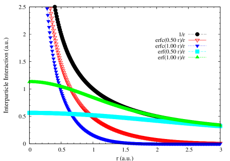
Figure 1: Interparticle interaction as a function of interparticle distance (in atomic units).

Traditionally, $f(r)$ is given by the Coulomb interaction $1/r$. However, in this work, we consider two types of $f(r)$: $\text{erf}(\omega r)/r$ and $\text{erfc}(\omega r)/r$, which are generated by splitting the Coulomb interaction into two components CASE ; CASE_MP2 . The former (the erf interaction) retains the long-range Coulomb tail without the singularity at $r=0$, while the latter (the erfc interaction) is a short-range interaction with a singularity at $r=0$. Physically, $1/\omega$ specifies the distance beyond which $\text{erf}(\omega r)/r$ approaches $1/r$ and the distance beyond which $\text{erfc}(\omega r)/r$ becomes insignificant (see Figure 1). Similar to the Coulomb case Boys ; Gauss , the nuclear-attraction and two-electron repulsion integrals modified for the erf and erfc interaction operators can be evaluated analytically over Gaussian basis functions Gauss ; erf_anal ; erf_anal2 , facilitating an efficient evaluation of the integrals needed for solving Eq. (3) and the equations associated with related approximate methods (see below). In principle, other types of $f(r)$ can also be adopted erf_anal ; erfgau_anal ; terf_anal ; op ; terf_JAP .

Similar to the Coulomb case, solving Eq. (3) for a given $f(r)$ is, however, extremely difficult even for the ground-state energy and wavefunction of a very small system, due to the prohibitively expensive computational cost. Practically, one searches for approximate solutions to Eq. (3), obtained from ab initio wavefunction methods Jensen ; CASE ; CASE_MP2 ; PC , such as the Hartree-Fock (HF) theory, second-order Møller-Plesset perturbation theory (MP2), coupled-cluster theory with iterative singles and doubles (CCSD), and CCSD with a perturbative treatment of triple substitutions (CCSD(T)). Among them, the CCSD(T) method with a sufficiently large basis set is generally expected to provide highly accurate results for a variety of small- to medium-sized systems.

Alternatively, Kohn-Sham density functional theory (KS-DFT) KS , a popular method for the study of the ground-state properties of large systems, can also be employed. Similar to the Coulomb case, density functional approximations (DFAs), such as the local density approximation (LDA) and generalized-gradient approximations (GGAs), to the exchange-correlation (XC) energy functional for a given $f(r)$ are needed in the corresponding KS-DFT OD ; RevYang . Here, the LDA exchange energy functional for the erf interaction is obtained by subtracting the LDA exchange energy functional for the erfc interaction SR-LDAX from the LDA exchange energy functional for the Coulomb interaction LDAX , whereas the LDA correlation energy functional for the erfc interaction is obtained by subtracting the LDA correlation energy functional for the erf interaction LR-LDAC from the LDA correlation energy functional for the Coulomb interaction LDAC . In addition, as the Perdew-Burke-Ernzerhof (PBE) XC energy functional (i.e., a popular GGA) for the Coulomb interaction PBE and its variant for the erfc interaction SR-PBE are both available, their difference gives the PBE XC energy functional for the erf interaction.

To illustrate how the nature of vdW interactions in rare-gas dimers changes with varying interparticle interactions, we calculate the potential energy curves of the He-He dimer associated with the interparticle interactions $\text{erf}(\omega r)/r$ ($\omega$ = $\infty$, 10.00, 2.00, 1.70, 1.40, and 1.10 bohr^-1) and $\text{erfc}(\omega r)/r$ ($\omega$ = 0.00, 0.10, 0.20, 0.25, 0.30, and 0.40 bohr^-1), using the corresponding CCSD(T), CCSD, MP2, HF, and KS-DFT employing the PBE and LDA XC energy functionals for the associated interactions Jensen ; CASE ; CASE_MP2 ; PC .

All calculations are performed with a development version of Q-Chem 4.0 Q-Chem . Results are computed using a large aug-cc-pVQZ basis set AQZ with a high-quality EML(250,590) grid, consisting of 250 Euler-Maclaurin radial grid points EM and 590 Lebedev angular grid points L . The counterpoise correction CP is employed to reduce basis set superposition error (BSSE).

III Results and Discussion

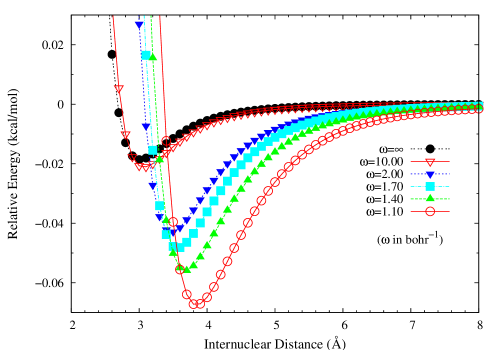
Figure 2: Potential energy curves of the He-He dimer associated with the long-range interparticle interactions $\text{erf}(\omega r)/r$, calculated using the corresponding CCSD(T). The $\omega=\infty$ case is equivalent to the Coulomb interaction $1/r$.

The potential energy curves of the He-He dimer associated with the long-range interparticle interactions $\text{erf}(\omega r)/r$, calculated using the corresponding CCSD(T), are presented in Figure 2. Similar to the Coulomb case (i.e., the $\omega=\infty$ case of the erf interaction), all the potential energy curves resemble the LJ potentials. For a smaller $\omega$, the strength of the erf interaction is weaker. Consequently, the electrons are more loosely bound to the nucleus, and the atoms are more polarizable, yielding larger values of $\sigma$ and $\epsilon$, respectively (see Eq. (1)) Jensen . Owing to the long-range nature of the erf interaction, the attractive vdW interaction is shown to have the $[\text{erf}(\omega R)]^{2}R^{-6}$ asymptote (essentially retaining the $R^{-6}$ asymptote of conventional vdW interactions) at sufficiently large internuclear distances $R$, based on a second-order perturbation theory (see the Appendix).

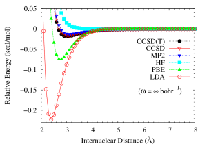
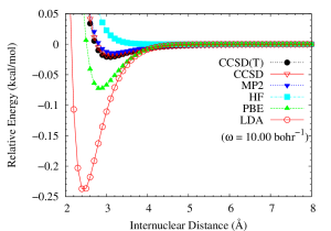
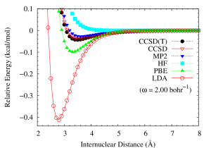
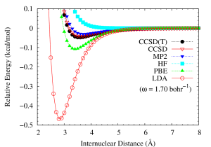
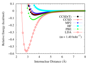
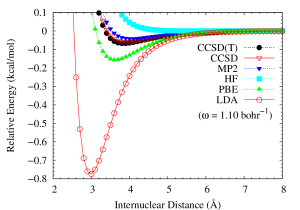
Figure 3: Potential energy curves of the He-He dimer associated with the long-range interparticle interactions $\text{erf}(\omega r)/r$, calculated using the corresponding CCSD(T), CCSD, MP2, HF, PBE, and LDA. The $\omega=\infty$ case is equivalent to the Coulomb interaction $1/r$.

In comparison with the highly accurate CCSD(T) results, the He-He potential energy curves associated with the erf interactions, calculated using the corresponding CCSD, MP2, HF, PBE, and LDA are presented in Figure 3. As shown, CCSD performs similarly to CCSD(T), and slightly outperforms MP2. Besides, CCSD(T), CCSD, and MP2 exhibit the correct $R^{-6}$ vdW asymptotes. By contrast, due to the lack of electron correlation, HF completely fails to describe the attractive vdW interactions, yielding purely repulsive potential energy curves for all the $\omega$ values studied. Within the framework of KS-DFT, PBE consistently outperforms LDA. However, in view of the large errors associated with the vdW minima and the incorrect vdW asymptotes (decaying much faster than $R^{-6}$) vdWDF ; vdWasymp , LDA, PBE, and possibly other semilocal density functionals semilocal cannot accurately describe long-range vdW interactions Dobson , wherein a fully nonlocal XC energy functional should be essential OD ; RevYang ; vdWDF .

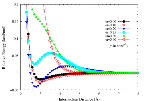
Figure 4: Potential energy curves of the He-He dimer associated with the short-range interparticle interactions $\text{erfc}(\omega r)/r$, calculated using the corresponding CCSD(T). The $\omega=0$ case is equivalent to the Coulomb interaction $1/r$.

On the other hand, the potential energy curves of the He-He dimer associated with the short-range interparticle interactions $\text{erfc}(\omega r)/r$, calculated using the corresponding CCSD(T), are shown in Figure 4. In contrast to the Coulomb case (i.e., the $\omega=0$ case of the erfc interaction), the potential energy curves show strong $\omega$-dependence. It resembles the LJ potential only for a vanishingly small $\omega$, displays a metastable state for an intermediate $\omega$ (around 0.25 bohr^-1 or smaller), and becomes purely repulsive for a $\omega$ larger than 0.30 bohr^-1 (see the Appendix).

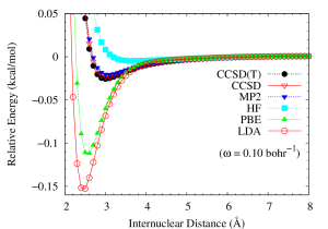
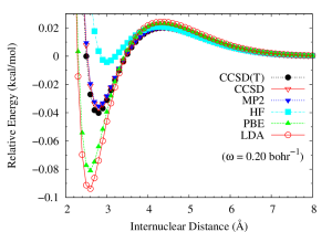
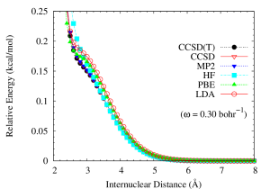
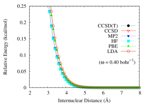
Figure 5: Potential energy curves of the He-He dimer associated with the short-range interparticle interactions $\text{erfc}(\omega r)/r$, calculated using the corresponding CCSD(T), CCSD, MP2, HF, PBE, and LDA. The $\omega=0$ case is equivalent to the Coulomb interaction $1/r$.

For comparison, the He-He potential energy curves associated with the erfc interactions, calculated using the corresponding CCSD, MP2, HF, PBE, and LDA are shown in Figure 5. With the increase of $\omega$, the potential energy curves obtained from all the computational methods become very similar. As would be expected on physical grounds, semilocal density functionals can be surprisingly accurate for short-range XC effects semilocal . PBE is shown to consistently perform better than LDA. Besides, due to the dominance of exchange-repulsion energy for a sufficiently large $\omega$, even the HF theory can be reliably accurate.

Similar to the Coulomb case, the overall trends of LDA and PBE are opposite to those of HF and MP2, implying that a combination of the HF exchange, MP2 correlation, and DFAs (e.g., LDA or GGAs) in KS-DFT (i.e., hybrid DFT hybrid or double-hybrid DFT B2PLYP ) may achieve a more favorable balance between cost and performance than CCSD(T) for the vdW interactions in large rare-gas dimers under the erf and erfc interactions.

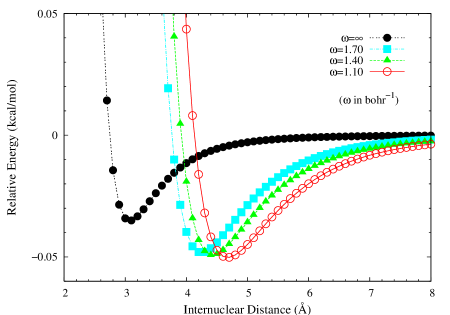
Figure 6: Potential energy curves of the He-Ne dimer associated with the long-range interparticle interactions $\text{erf}(\omega r)/r$, calculated using the corresponding CCSD(T). The $\omega=\infty$ case is equivalent to the Coulomb interaction $1/r$.

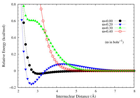
Figure 7: Potential energy curves of the He-Ne dimer associated with the short-range interparticle interactions $\text{erfc}(\omega r)/r$, calculated using the corresponding CCSD(T). The $\omega=0$ case is equivalent to the Coulomb interaction $1/r$.

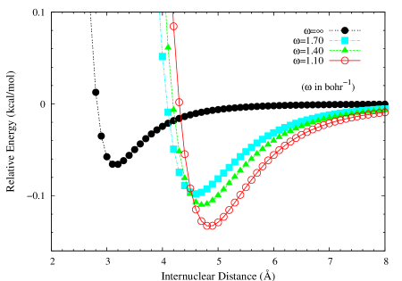
Figure 8: Potential energy curves of the Ne-Ne dimer associated with the long-range interparticle interactions $\text{erf}(\omega r)/r$, calculated using the corresponding CCSD(T). The $\omega=\infty$ case is equivalent to the Coulomb interaction $1/r$.

In addition, we calculate the potential energy curves of the He-Ne and Ne-Ne dimers associated with the erf and erfc interactions, using the corresponding CCSD(T), as shown in Figures 6, 7, 8 and 9. For the Coulomb case, the values of $\sigma$ for the He-Ne and Ne-Ne dimers are larger than that for the He-He dimer. Nevertheless, similar trends are also found for the potential energy curves of the He-Ne, Ne-Ne, and possibly other rare-gas dimers.

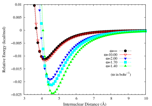
Figure 10: Potential energy curves for the lowest triplet states of H₂ associated with the long-range interparticle interactions $\text{erf}(\omega r)/r$, calculated using the corresponding CCSD. The $\omega=\infty$ case is equivalent to the Coulomb interaction $1/r$.

To test the transferability of the above observed trends for other vdW systems, we calculate the potential energy curves for the lowest triplet states of H₂ (a simple vdW system) tH2 associated with the erf and erfc interactions, using the corresponding CCSD (i.e., an exact theory for any two-electron system). As shown in Figures 10 and 11, the major features of the potential energy curves remain very similar to those found for rare-gas dimers.

Here we comment on the connection between this study and long-range corrected (LC) hybrid functionals for systems with Coulomb interactions LC-DFT ; LCHirao ; CAM-B3LYP ; LC-wPBE ; BNL ; wB97X ; wB97X-D ; Herbert ; wB97X-2 ; M11 ; wM05-D ; LC-D3 . These functionals model the short-range interaction (e.g., the erfc interaction) by a DFA in KS-DFT and the complementary long-range interaction (e.g., the erf interaction) by HF exchange or a fully nonlocal (i.e., orbital-dependent) XC energy component from ab initio wavefunction methods. In Figures 3 and 5, compared to the highly accurate CCSD(T) results, LDA and PBE perform reasonably well for sufficiently short-range interparticle interactions, whereas they perform poorly for long-range interparticle interactions. Accordingly, our findings are also in support of the key feature of the LC hybrid functionals for systems with Coulomb interactions, which have recently been found to provide supreme performance for a very wide range of applications LCAC ; EB , especially for problems related to the asymptote of the XC potential exactip ; asymp ; LB94 ; sum_vxc2 ; sum_vxc3 ; Staroverov ; AC1 ; LFA , self-interaction errors SIC ; SIE , fundamental gaps DD1 ; DD2 ; DD2a ; DD4a ; DDcorr ; DD6 ; DD7 ; errsinfuncs ; DD8 ; DDHirao ; GKS2 ; Correction2 ; Correction3 ; DDChai , and charge-transfer excitations Dreuw ; Tozer ; Gritsenko ; Dreuw2 ; Dreuw3 ; fxcd ; Peng . Besides, empirical atom-atom dispersion potentials DFT-D1 ; DFT-D2 ; DFT-D3 ; wB97X-D ; wM05-D ; LC-D3 or MP2 correlation energy B2PLYP ; wB97X-2 ; PBE0-DH ; PBE0-2 ; SCAN0-2 can be added to the KS-DFT energy in order to improve the description of noncovalent interactions (e.g., vdW interactions). Alternatively, KS-DFT may also be combined with symmetry-adapted perturbation theory (SAPT) SAPT ; SAPT1 ; SAPT2 ; SAPT3 ; SAPT4 ; SAPT5 ; SAPT6 ; SAPT7 ; SAPT8 to yield accurate results for noncovalent interactions SAPT_DFT ; SAPT_DFT1 ; SAPT_DFT2 ; SAPT_DFT3 ; SAPT_DFT4 ; SAPT_DFT5 ; SAPT_DFT6 . In addition, to properly describe strong static correlation, it could be essential to develop a combined LC hybrid scheme with random phase approximations (RPAs) OD ; Perdew09 ; RPA_Yang ; RPA_Yang2 for small- to medium-sized systems or with thermally-assisted-occupation density functional theory (TAO-DFT) TAO-DFT ; TAO-DFT2 ; TAO-DFT3 for large-sized systems.

IV Conclusions

In conclusion, we have developed a comprehensive understanding of the physics involved in controlling the vdW interactions in rare-gas dimers. Specifically, we have examined the potential energy curves of the rare-gas dimers associated with a variety of interparticle interactions, using the highly accurate CCSD(T) method as well as other computational methods. The long-range interparticle interactions are shown to be essential for retaining the main features of conventional vdW interactions, which cannot be properly described by LDA, PBE, and possibly other semilocal density functionals in KS-DFT, but can be accurately described by MP2, CCSD, and possibly other fully nonlocal XC energy components from ab initio wavefunction methods. On the other hand, the nature of vdW interactions is shown to change drastically with the short-range interparticle interactions, wherein LDA, PBE, and possibly other semilocal density functionals in KS-DFT perform reasonably well for sufficiently short-range interparticle interactions (e.g., $\text{erfc}(\omega r)/r$ with $\omega$ = 0.30 bohr^-1 or larger). Therefore, our findings also support the main feature of the LC hybrid functionals for systems with Coulomb interactions. Although only the vdW interactions in rare-gas dimers and the triplet H₂ molecule are studied and discussed in this work, our conclusion may remain appropriate for other vdW-dominated systems.

Appendix: Asymptote of the interaction energy curve between two well-separated rare-gas atoms associated with the long-range (erf) interparticle interactions

Similar to the derivation for the Coulomb case (e.g., see Chapter 3 of Ref. vdW2 ), we derive an analytical expression for the asymptote of the interaction energy curve between two well-separated rare-gas atoms associated with the long-range interparticle (nuclear-electron, electron-electron, and nuclear-nuclear) interaction operator $f(r)$: $\text{erf}(\omega r)/r$ (the erf interaction), based on a second-order perturbation theory PT . Since in the Coulomb case, a rare-gas atom has no permanent multipole moments in its nondegenerate ground state MM , presumably this remains correct for the erf interaction with a sufficiently large $\omega$ or for the erfc interaction [$f(r)$: $\text{erfc}(\omega r)/r$] with a sufficiently small $\omega$. Note also that the finite speed of propagation of electromagnetic signals is not taken into account in our derivation vdW2 . For brevity, the Einstein summation convention ESC is adopted here. Based on this convention, when an index variable appears twice in a term, it implies a summation of that term over all possible values of the index.

Consider a rare-gas atom $A$, composed of a nucleus situated at $\mathbf{r}_{\alpha=0}$ and $N_{A}$ electrons situated at $\mathbf{r_{\alpha}}$ ($\alpha=1,2,...,N_{A}$) with respect to the nucleus of $A$. The electric potential at a point $\mathbf{r}$, due to the charge distribution, is

$$V_{A}(\mathbf{r})=\frac{1}{4\pi\epsilon_{0}}\sum\limits_{\alpha=0}^{N_{A}}e^{A}_{\alpha}f(|\mathbf{r}-\mathbf{r_{\alpha}}|),$$ (5)

where $e^{A}_{\alpha=0}=N_{A}e$ is the nuclear charge of $A$, and $e^{A}_{\alpha}=-e$ ($\alpha=1,2,...,N_{A}$) is the charge of an electron. The Taylor series expansion of $V_{A}(\mathbf{r})$ around the nucleus of $A$ gives

$$\begin{split}V_{A}(\mathbf{r})&=\frac{1}{4\pi\epsilon_{0}}\bigg{[}\sum\limits_{\alpha}e^{A}_{\alpha}f(r)-\sum\limits_{\alpha}e^{A}_{\alpha}r_{i\alpha}\nabla_{i}f(r)+\frac{1}{2!}\sum\limits_{\alpha}e^{A}_{\alpha}r_{i\alpha}r_{j\alpha}\nabla_{i}\nabla_{j}f(r)+\cdots\bigg{]}\\ &=\frac{1}{4\pi\epsilon_{0}}\bigg{[}e^{A}_{tot}-\mu^{A}_{i}\nabla_{i}+Q^{A}_{ij}\nabla_{i}\nabla_{j}+\cdots\bigg{]}f(r),\end{split}$$ (6)

where the first term is from an electric monopole $e^{A}_{tot}=\sum\limits_{\alpha}e^{A}_{\alpha}$, the second term is from an electric dipole, whose $i^{th}$ Cartesian component $\mu^{A}_{i}=\sum\limits_{\alpha}e^{A}_{\alpha}r_{i\alpha}$, the third term is from an electric quadrupole source, $Q^{A}_{ij}=\frac{1}{2!}\sum\limits_{\alpha}e^{A}_{\alpha}r_{i\alpha}r_{j\alpha}$, and so on.

Consider a second rare-gas atom $B$, composed of a nucleus situated at $\mathbf{r}_{\beta=0}$ and $N_{B}$ electrons situated at $\mathbf{r_{\beta}}$ ($\beta=1,2,...,N_{B}$) with respect to the nucleus of $B$. Let $\mathbf{R}$ be the separation distance vector pointing from the nucleus of $A$ towards the nucleus of $B$. The interaction energy between atoms $A$ and $B$ is

$$U_{AB}=\sum\limits_{\beta=0}^{N_{B}}e^{B}_{\beta}V_{A}(\mathbf{R}+\mathbf{r_{\beta}}),$$ (7)

where $e^{B}_{\beta=0}=N_{B}e$ is the nuclear charge of $B$, and $e^{B}_{\beta}=-e$ ($\beta=1,2,...,N_{B}$) is the charge of an electron. The Taylor series expansion of $V_{A}(\mathbf{R}+\mathbf{r_{\beta}})$ around the nucleus of $B$ gives

$$\begin{split}V_{A}(\mathbf{R}+\mathbf{r_{\beta}})&=V_{A}(\mathbf{R})+r_{i\beta}\nabla_{i}V_{A}(\mathbf{R})+\frac{1}{2!}r_{i\beta}r_{j\beta}\nabla_{i}\nabla_{j}V_{A}(\mathbf{R})+\cdots\\ &=\bigg{[}1+r_{i\beta}\nabla_{i}+\frac{1}{2!}r_{i\beta}r_{j\beta}\nabla_{i}\nabla_{j}+\cdots\bigg{]}V_{A}(\mathbf{R}).\end{split}$$ (8)

Substituting Eq. (6) and Eq. (8) into Eq. (7) produces

$$\begin{split}U_{AB}&=\sum\limits_{\beta}e^{B}_{\beta}\bigg{[}1+r_{i\beta}\nabla_{i}+\frac{1}{2!}r_{i\beta}r_{j\beta}\nabla_{i}\nabla_{j}+\cdots\bigg{]}V_{A}(\mathbf{R})\\ &=\bigg{[}e^{B}_{tot}+\mu^{B}_{i}\nabla_{i}+Q^{B}_{ij}\nabla_{i}\nabla_{j}+\cdots\bigg{]}\frac{1}{4\pi\epsilon_{0}}\bigg{[}e^{A}_{tot}-\mu^{A}_{i}\nabla_{i}+Q^{A}_{ij}\nabla_{i}\nabla_{j}+\cdots\bigg{]}f(R)\\ &=\frac{1}{4\pi\epsilon_{0}}\bigg{[}e^{A}_{tot}e^{B}_{tot}+\bigg{(}e^{A}_{tot}\mu^{B}_{i}\nabla_{i}-e^{B}_{tot}\mu^{A}_{i}\nabla_{i}\bigg{)}-\mu^{A}_{i}\mu^{B}_{j}\nabla_{i}\nabla_{j}+\bigg{(}e^{A}_{tot}Q^{B}_{ij}\nabla_{i}\nabla_{j}+e^{B}_{tot}Q^{A}_{ij}\nabla_{i}\nabla_{j}\bigg{)}\\ &\ \ -\bigg{(}\mu^{A}_{i}Q^{B}_{jk}\nabla_{i}\nabla_{j}\nabla_{k}-\mu^{B}_{i}Q^{A}_{jk}\nabla_{i}\nabla_{j}\nabla_{k}\bigg{)}+Q^{A}_{ij}Q^{B}_{kl}\nabla_{i}\nabla_{j}\nabla_{k}\nabla_{l}+\cdots\bigg{]}f(R).\end{split}$$ (9)

Here $e^{B}_{tot}=\sum\limits_{\beta}e^{B}_{\beta}$, $\mu^{B}_{i}=\sum\limits_{\beta}e^{B}_{\beta}r_{i\beta}$, $Q^{B}_{ij}=\frac{1}{2!}\sum\limits_{\beta}e^{B}_{\beta}r_{i\beta}r_{j\beta}$, and so on. Since atoms $A$ and $B$ are both neutral, $e^{A}_{tot}=e^{B}_{tot}=0$. Accordingly,

$$U_{AB}=\frac{1}{4\pi\epsilon_{0}}\bigg{[}-\mu^{A}_{i}\mu^{B}_{j}\nabla_{i}\nabla_{j}-\bigg{(}\mu^{A}_{i}Q^{B}_{jk}-\mu^{B}_{i}Q^{A}_{jk}\bigg{)}\nabla_{i}\nabla_{j}\nabla_{k}+Q^{A}_{ij}Q^{B}_{kl}\nabla_{i}\nabla_{j}\nabla_{k}\nabla_{l}+\cdots\bigg{]}f(R)$$ (10)

can be expressed as a sum of dipole-dipole (dd), dipole-quadrupole (dq), quadrupole-quadrupole (qq), and other contributions.

To evaluate the interaction energy between ground-state rare-gas atoms $A$ and $B$, the classical interaction energy given by Eq. (10) should be first converted into quantum mechanical operator. Perturbation theory may then be adopted to obtain the various perturbation contributions to the interaction energy at large $R$.

Let the Hamiltonian of an isolated rare-gas atom $X$ ($X$ = $A$, $B$) be $H^{X}$. The Schrödinger equation

$$H^{X}\psi^{X}_{n}=E^{X}_{n}\psi^{X}_{n}$$ (11)

is solved for the $n^{th}$ excited-state energy $E^{X}_{n}$ and wavefunction $\psi^{X}_{n}$, where the $n=0$ case refers to the ground state. Accordingly, the full Hamiltonian of rare-gas atoms $A$ and $B$ can be expressed as

$$H=H^{A}+H^{B}+U_{AB}.$$ (12)

The interaction energy between ground-state rare-gas atoms $A$ and $B$ can be calculated as

$$\Delta E_{int}=E_{0}-(E^{A}_{0}+E^{B}_{0}),$$ (13)

where $E_{0}$ is the ground-state energy of $H$.

To circumvent the need for solving the Schrödinger equation with Hamiltonian $H$, $E_{0}$ may be expressed in terms of $\{E^{A}_{n},\psi^{A}_{n};E^{B}_{n},\psi^{B}_{n}\}$, based on perturbation theory vdW2 ; PT . Since atoms $A$ and $B$ are well-separated, an appropriate unperturbed Hamiltonian is the sum of the Hamiltonians of the isolated atoms $A$ and $B$,

$$H_{0}=H^{A}+H^{B}.$$ (14)

Consequently,

$$H=H_{0}+U_{AB},$$ (15)

where $U_{AB}$ given by Eq. (10) is the perturbation.

IV.1 Zeroth-Order Theory

$H_{0}\Psi^{(0)}_{n}=E^{(0)}_{n}\Psi^{(0)}_{n}$. At large $R$, the effects of electron exchange are insignificant. Accordingly, for the $n^{th}$ excited state, $\Psi^{(0)}_{n}=\psi^{A}_{r}\psi^{B}_{s}$ and $E^{(0)}_{n}=E^{A}_{r}+E^{B}_{s}$, where the isolated atoms $A$ and $B$ are described by quantum numbers $r$ and $s$, respectively. For the ground state, $\Psi^{(0)}_{0}=\psi^{A}_{0}\psi^{B}_{0}$ and $E^{(0)}_{0}=E^{A}_{0}+E^{B}_{0}$. Correspondingly, $\Delta E_{int}=E_{0}-(E^{A}_{0}+E^{B}_{0})\approx(E^{(0)}_{0})-(E^{A}_{0}+E^{B}_{0})=(E^{A}_{0}+E^{B}_{0})-(E^{A}_{0}+E^{B}_{0})=0$. Therefore, to obtain a nonvanishing $\Delta E_{int}$, it is necessary to go beyond the zeroth-order theory.

IV.2 First-Order Theory

$E^{(1)}_{n}=\langle\Psi^{(0)}_{n}|U_{AB}|\Psi^{(0)}_{n}\rangle$. Since in the Coulomb case, the isolated rare-gas atom $X$ ($X$ = $A$, $B$) has no permanent multipole moments in its nondegenerate ground state MM , presumably this holds true for the erf interaction with a sufficiently large $\omega$ or for the erfc interaction with a sufficiently small $\omega$. Accordingly, the dipole terms are vanished $\langle\psi^{X}_{0}|\mu^{X}_{i}|\psi^{X}_{0}\rangle=0$, the quadrupole terms are vanished $\langle\psi^{X}_{0}|Q^{X}_{ij}|\psi^{X}_{0}\rangle=0$, and so on. Therefore, the first-order correction to the ground-state energy is

$$\begin{split}E^{(1)}_{0}&=\langle\Psi^{(0)}_{0}|U_{AB}|\Psi^{(0)}_{0}\rangle\\ &=\langle\Psi^{(0)}_{0}|\frac{1}{4\pi\epsilon_{0}}\bigg{[}-\mu^{A}_{i}\mu^{B}_{j}\nabla_{i}\nabla_{j}-\bigg{(}\mu^{A}_{i}Q^{B}_{jk}-\mu^{B}_{i}Q^{A}_{jk}\bigg{)}\nabla_{i}\nabla_{j}\nabla_{k}+Q^{A}_{ij}Q^{B}_{kl}\nabla_{i}\nabla_{j}\nabla_{k}\nabla_{l}+\cdots\bigg{]}f(R)|\Psi^{(0)}_{0}\rangle\\ &=-\frac{1}{4\pi\epsilon_{0}}\bigg{[}\nabla_{i}\nabla_{j}f(R)\langle\Psi^{(0)}_{0}|\mu^{A}_{i}\mu^{B}_{j}|\Psi^{(0)}_{0}\rangle+\nabla_{i}\nabla_{j}\nabla_{k}f(R)\langle\Psi^{(0)}_{0}|\bigg{(}\mu^{A}_{i}Q^{B}_{jk}-\mu^{B}_{i}Q^{A}_{jk}\bigg{)}|\Psi^{(0)}_{0}\rangle\\ &\ \ -\nabla_{i}\nabla_{j}\nabla_{k}\nabla_{l}f(R)\langle\Psi^{(0)}_{0}|Q^{A}_{ij}Q^{B}_{kl}|\Psi^{(0)}_{0}\rangle+\cdots\bigg{]}\\ &=-\frac{1}{4\pi\epsilon_{0}}\bigg{[}\nabla_{i}\nabla_{j}f(R)\langle\psi^{A}_{0}\psi^{B}_{0}|\mu^{A}_{i}\mu^{B}_{j}|\psi^{A}_{0}\psi^{B}_{0}\rangle+\nabla_{i}\nabla_{j}\nabla_{k}f(R)\langle\psi^{A}_{0}\psi^{B}_{0}|\bigg{(}\mu^{A}_{i}Q^{B}_{jk}-\mu^{B}_{i}Q^{A}_{jk}\bigg{)}|\psi^{A}_{0}\psi^{B}_{0}\rangle\\ &\ \ -\nabla_{i}\nabla_{j}\nabla_{k}\nabla_{l}f(R)\langle\psi^{A}_{0}\psi^{B}_{0}|Q^{A}_{ij}Q^{B}_{kl}|\psi^{A}_{0}\psi^{B}_{0}\rangle+\cdots\bigg{]}\\ &=-\frac{1}{4\pi\epsilon_{0}}\bigg{[}\nabla_{i}\nabla_{j}f(R)\langle\psi^{A}_{0}|\mu^{A}_{i}|\psi^{A}_{0}\rangle\langle\psi^{B}_{0}|\mu^{B}_{j}|\psi^{B}_{0}\rangle\\ &\ \ +\nabla_{i}\nabla_{j}\nabla_{k}f(R)\bigg{(}\langle\psi^{A}_{0}|\mu^{A}_{i}|\psi^{A}_{0}\rangle\langle\psi^{B}_{0}|Q^{B}_{jk}|\psi^{B}_{0}\rangle-\langle\psi^{B}_{0}|\mu^{B}_{i}|\psi^{B}_{0}\rangle\langle\psi^{A}_{0}|Q^{A}_{jk}|\psi^{A}_{0}\rangle\bigg{)}\\ &\ \ -\nabla_{i}\nabla_{j}\nabla_{k}\nabla_{l}f(R)\langle\psi^{A}_{0}|Q^{A}_{ij}|\psi^{A}_{0}\rangle\langle\psi^{B}_{0}|Q^{B}_{kl}|\psi^{B}_{0}\rangle+\cdots\bigg{]}=0.\end{split}$$ (16)

Accordingly, $\Delta E_{int}=E_{0}-(E^{A}_{0}+E^{B}_{0})\approx(E^{(0)}_{0}+E^{(1)}_{0})-(E^{A}_{0}+E^{B}_{0})=E^{(1)}_{0}=0$. Therefore, to obtain a nonvanishing $\Delta E_{int}$, it is also necessary to go beyond the first-order theory.

IV.3 Second-Order Theory

$E^{(2)}_{n}=-\sum\limits_{m\neq n}\frac{|\langle\Psi^{(0)}_{m}|U_{AB}|\Psi^{(0)}_{n}\rangle|^{2}}{E^{(0)}_{m}-E^{(0)}_{n}}$. The second-order correction to the ground-state energy is

$$E^{(2)}_{0}=-\sum\limits_{m\neq 0}\frac{|\langle\Psi^{(0)}_{m}|U_{AB}|\Psi^{(0)}_{0}\rangle|^{2}}{E^{(0)}_{m}-E^{(0)}_{0}},$$ (17)

which is always nonpositive.

From Eq. (10), if only the dipole-dipole contribution is retained, we have

$$U_{AB}^{dd}=-\frac{1}{4\pi\epsilon_{0}}\mu^{A}_{i}\mu^{B}_{j}\nabla_{i}\nabla_{j}f(R).$$ (18)

Accordingly, the second-order correction to the ground-state energy due to the dipole-dipole contribution is

$$\begin{split}E^{(2),dd}_{0}&=-\sum\limits_{m\neq 0}\frac{|\langle\Psi^{(0)}_{m}|U_{AB}^{dd}|\Psi^{(0)}_{0}\rangle|^{2}}{E^{(0)}_{m}-E^{(0)}_{0}}=-\sum\limits_{m\neq 0}\frac{|\langle\Psi^{(0)}_{m}|(-\frac{1}{4\pi\epsilon_{0}})\mu^{A}_{i}\mu^{B}_{j}\nabla_{i}\nabla_{j}f(R)|\Psi^{(0)}_{0}\rangle|^{2}}{E^{(0)}_{m}-E^{(0)}_{0}}\\ &=-\frac{1}{(4\pi\epsilon_{0})^{2}}\sum\limits_{r\neq 0}\sum\limits_{s\neq 0}\frac{|\langle\psi^{A}_{r}\psi^{B}_{s}|\mu^{A}_{i}\mu^{B}_{j}\nabla_{i}\nabla_{j}f(R)|\psi^{A}_{0}\psi^{B}_{0}\rangle|^{2}}{E^{A}_{r}+E^{B}_{s}-E^{A}_{0}-E^{B}_{0}}\\ &=-\frac{1}{(4\pi\epsilon_{0})^{2}}\sum\limits_{r\neq 0}\sum\limits_{s\neq 0}\frac{\langle\psi^{A}_{r}\psi^{B}_{s}|\mu^{A}_{i}\mu^{B}_{j}\nabla_{i}\nabla_{j}f(R)|\psi^{A}_{0}\psi^{B}_{0}\rangle\langle\psi^{A}_{0}\psi^{B}_{0}|\mu^{A}_{i^{\prime}}\mu^{B}_{j^{\prime}}\nabla_{i^{\prime}}\nabla_{j^{\prime}}f(R)|\psi^{A}_{r}\psi^{B}_{s}\rangle}{E^{A}_{r}+E^{B}_{s}-E^{A}_{0}-E^{B}_{0}}\\ &=-\frac{1}{(4\pi\epsilon_{0})^{2}}[\nabla_{i}\nabla_{j}f(R)][\nabla_{i^{\prime}}\nabla_{j^{\prime}}f(R)]\sum\limits_{r\neq 0}\sum\limits_{s\neq 0}\frac{\langle\psi^{A}_{r}\psi^{B}_{s}|\mu^{A}_{i}\mu^{B}_{j}|\psi^{A}_{0}\psi^{B}_{0}\rangle\langle\psi^{A}_{0}\psi^{B}_{0}|\mu^{A}_{i^{\prime}}\mu^{B}_{j^{\prime}}|\psi^{A}_{r}\psi^{B}_{s}\rangle}{E^{A}_{r}+E^{B}_{s}-E^{A}_{0}-E^{B}_{0}}\\ &=-\frac{1}{(4\pi\epsilon_{0})^{2}}[\nabla_{i}\nabla_{j}f(R)][\nabla_{i^{\prime}}\nabla_{j^{\prime}}f(R)]\\ &\ \ \times\sum\limits_{r\neq 0}\sum\limits_{s\neq 0}\frac{\langle\psi^{A}_{r}|\mu^{A}_{i}|\psi^{A}_{0}\rangle\langle\psi^{B}_{s}|\mu^{B}_{j}|\psi^{B}_{0}\rangle\langle\psi^{A}_{0}|\mu^{A}_{i^{\prime}}|\psi^{A}_{r}\rangle\langle\psi^{B}_{0}|\mu^{B}_{j^{\prime}}|\psi^{B}_{s}\rangle}{E^{A}_{r}+E^{B}_{s}-E^{A}_{0}-E^{B}_{0}}.\end{split}$$ (19)

In Eq. (19), the ($r=0,s\neq 0$) and ($r\neq 0,s=0$) terms are excluded in the summation, due to the vanishing dipole terms, i.e., $\langle\psi^{X}_{0}|\mu^{X}_{i}|\psi^{X}_{0}\rangle=0$ ($X$ = $A$, $B$).

• For the erf interaction, $f(R)=\frac{\operatorname{erf}(\omega R)}{R}$.

  $$\begin{split}\nabla_{i}\nabla_{j}f(R)&=\nabla_{i}\nabla_{j}\frac{\operatorname{erf}(\omega R)}{R}=\nabla_{i}\bigg{[}\frac{1}{R}\nabla_{j}\operatorname{erf}(\omega R)+\operatorname{erf}(\omega R)\nabla_{j}\frac{1}{R}\bigg{]}\\ &=\nabla_{i}\bigg{[}\frac{1}{R}\frac{\partial\operatorname{erf}(\omega R)}{\partial R}\hat{R}_{j}-\frac{\operatorname{erf}(\omega R)}{R^{2}}\hat{R}_{j}\bigg{]}=\nabla_{i}\bigg{[}\frac{1}{R^{2}}\frac{\partial\operatorname{erf}(\omega R)}{\partial R}R_{j}-\frac{\operatorname{erf}(\omega R)}{R^{3}}R_{j}\bigg{]}\\ &=\frac{\partial}{\partial R}\bigg{[}\frac{1}{R^{2}}\frac{\partial\operatorname{erf}(\omega R)}{\partial R}\bigg{]}\hat{R}_{i}R_{j}+\frac{1}{R^{2}}\frac{\partial\operatorname{erf}(\omega R)}{\partial R}\delta_{ij}-\frac{\partial}{\partial R}\bigg{[}\frac{\operatorname{erf}(\omega R)}{R^{3}}\bigg{]}\hat{R}_{i}R_{j}-\frac{\operatorname{erf}(\omega R)}{R^{3}}\delta_{ij}\\ &=R\bigg{\{}\frac{\partial}{\partial R}\bigg{[}\frac{1}{R^{2}}\frac{\partial\operatorname{erf}(\omega R)}{\partial R}-\frac{\operatorname{erf}(\omega R)}{R^{3}}\bigg{]}\bigg{\}}\hat{R}_{i}\hat{R}_{j}+\bigg{[}\frac{1}{R^{2}}\frac{\partial\operatorname{erf}(\omega R)}{\partial R}-\frac{\operatorname{erf}(\omega R)}{R^{3}}\bigg{]}\delta_{ij}\\ &=\bigg{[}-\frac{4\omega}{\sqrt{\pi}}\frac{1}{R^{2}}e^{-\omega^{2}R^{2}}-\frac{4\omega^{3}}{\sqrt{\pi}}e^{-\omega^{2}R^{2}}+\frac{3}{R^{3}}\operatorname{erf}(\omega R)-\frac{1}{R^{2}}\frac{2\omega}{\sqrt{\pi}}e^{-\omega^{2}R^{2}}\bigg{]}\hat{R}_{i}\hat{R}_{j}\\ &\ \ +\bigg{[}\frac{2\omega}{\sqrt{\pi}}\frac{1}{R^{2}}e^{-\omega^{2}R^{2}}-\frac{\operatorname{erf}(\omega R)}{R^{3}}\bigg{]}\delta_{ij}.\end{split}$$ (20)

  Since $e^{-\omega^{2}R^{2}}$ decays faster than polynomials when $R$ is large,
  $\nabla_{i}\nabla_{j}f(R)\approx-\frac{\operatorname{erf}(\omega R)}{R^{3}}(\delta_{ij}-3\hat{R}_{i}\hat{R}_{j})$ at large $R$. Accordingly,

  $$\begin{split}E^{(2),dd}_{0}&\approx-\frac{1}{(4\pi\epsilon_{0})^{2}}\frac{[\operatorname{erf}(\omega R)]^{2}}{R^{6}}(\delta_{ij}-3\hat{R}_{i}\hat{R}_{j})(\delta_{i^{\prime}j^{\prime}}-3\hat{R}_{i^{\prime}}\hat{R}_{j^{\prime}})\\ &\ \ \times\sum\limits_{r\neq 0}\sum\limits_{s\neq 0}\frac{\langle\psi^{A}_{r}|\mu^{A}_{i}|\psi^{A}_{0}\rangle\langle\psi^{B}_{s}|\mu^{B}_{j}|\psi^{B}_{0}\rangle\langle\psi^{A}_{0}|\mu^{A}_{i^{\prime}}|\psi^{A}_{r}\rangle\langle\psi^{B}_{0}|\mu^{B}_{j^{\prime}}|\psi^{B}_{s}\rangle}{E^{A}_{r}+E^{B}_{s}-E^{A}_{0}-E^{B}_{0}}.\end{split}$$ (21)

  Similar to the Coulomb case (e.g., see Chapter 3 of Ref. vdW2 ), we adopt the rotational average of $\langle\psi^{A}_{r}|\mu^{A}_{i}|\psi^{A}_{0}\rangle\langle\psi^{A}_{0}|\mu^{A}_{i^{\prime}}|\psi^{A}_{r}\rangle$ = $\frac{1}{3}\delta_{ii^{\prime}}|\langle\psi^{A}_{r}|\mu^{A}|\psi^{A}_{0}\rangle|^{2}$, and the rotational average of $\langle\psi^{B}_{s}|\mu^{B}_{j}|\psi^{B}_{0}\rangle\langle\psi^{B}_{0}|\mu^{B}_{j^{\prime}}|\psi^{B}_{s}\rangle$ = $\frac{1}{3}\delta_{jj^{\prime}}|\langle\psi^{B}_{s}|\mu^{B}|\psi^{B}_{0}\rangle|^{2}$, where $\mu^{A}=\sum\limits_{\alpha}e^{A}_{\alpha}\mathbf{r_{\alpha}}$ and $\mu^{B}=\sum\limits_{\beta}e^{B}_{\beta}\mathbf{r_{\beta}}$. Also, note that

  $$\sum\limits_{i=1}^{3}\sum\limits_{j=1}^{3}\sum\limits_{i^{\prime}=1}^{3}\sum\limits_{j^{\prime}=1}^{3}(\delta_{ij}-3\hat{R}_{i}\hat{R}_{j})(\delta_{i^{\prime}j^{\prime}}-3\hat{R}_{i^{\prime}}\hat{R}_{j^{\prime}})\delta_{ii^{\prime}}\delta_{jj^{\prime}}=\sum\limits_{i=1}^{3}\sum\limits_{j=1}^{3}(\delta_{ij}-3\hat{R}_{i}\hat{R}_{j})^{2}=6.$$ (22)

  Therefore, from Eq. (21),

  $$E^{(2),dd}_{0}\approx-\frac{1}{24\pi^{2}\epsilon_{0}^{2}}\frac{[\operatorname{erf}(\omega R)]^{2}}{R^{6}}\sum\limits_{r\neq 0}\sum\limits_{s\neq 0}\frac{|\langle\psi^{A}_{r}|\mu^{A}|\psi^{A}_{0}\rangle|^{2}|\langle\psi^{B}_{s}|\mu^{B}|\psi^{B}_{0}\rangle|^{2}}{E^{A}_{r}+E^{B}_{s}-E^{A}_{0}-E^{B}_{0}}.$$ (23)

  From Eq. (10), retaining also the dipole-quadrupole, quadrupole-quadrupole, and other contributions will produce additional terms in Eq. (17), involving $\nabla_{i}\nabla_{j}\nabla_{k}f(R)$, $\nabla_{i}\nabla_{j}\nabla_{k}\nabla_{l}f(R)$, and so on. For the erf interaction, it can be shown that $\nabla_{i}\nabla_{j}f(R)$ decays more slowly than $\nabla_{i}\nabla_{j}\nabla_{k}f(R)$, and $\nabla_{i}\nabla_{j}\nabla_{k}f(R)$ decays more slowly than $\nabla_{i}\nabla_{j}\nabla_{k}\nabla_{l}f(R)$, and so on. Accordingly, $E^{(2)}_{0}\approx E^{(2),dd}_{0}$ at large $R$. Therefore, in the second-order theory, the interaction energy between rare-gas atoms $A$ and $B$ at large $R$ is

  $$\begin{split}\Delta E_{int}&=E_{0}-(E^{A}_{0}+E^{B}_{0})\approx(E^{(0)}_{0}+E^{(1)}_{0}+E^{(2)}_{0})-(E^{A}_{0}+E^{B}_{0})=E^{(2)}_{0}\approx E^{(2),dd}_{0}\\ &\approx-\frac{1}{24\pi^{2}\epsilon_{0}^{2}}\frac{[\operatorname{erf}(\omega R)]^{2}}{R^{6}}\sum\limits_{r\neq 0}\sum\limits_{s\neq 0}\frac{|\langle\psi^{A}_{r}|\mu^{A}|\psi^{A}_{0}\rangle|^{2}|\langle\psi^{B}_{s}|\mu^{B}|\psi^{B}_{0}\rangle|^{2}}{E^{A}_{r}+E^{B}_{s}-E^{A}_{0}-E^{B}_{0}},\end{split}$$ (24)

  which has the $[\text{erf}(\omega R)]^{2}R^{-6}$ asymptote.

• For the erfc interaction, $f(R)=\frac{\operatorname{erfc}(\omega R)}{R}$.

  In the second-order theory, the interaction energy between rare-gas atoms $A$ and $B$, $\Delta E_{int}=E_{0}-(E^{A}_{0}+E^{B}_{0})\approx E^{(2)}_{0}=-\sum\limits_{m\neq 0}\frac{|\langle\Psi^{(0)}_{m}|U_{AB}|\Psi^{(0)}_{0}\rangle|^{2}}{E^{(0)}_{m}-E^{(0)}_{0}}$, is always nonpositive. Therefore, it is necessary to go beyond the second-order theory to describe the repulsive interaction energy at large $R$ (as discussed in our paper), which is, however, beyond the scope of our discussion here.

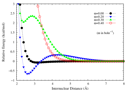
Figure 9: Potential energy curves of the Ne-Ne dimer associated with the short-range interparticle interactions $\text{erfc}(\omega r)/r$, calculated using the corresponding CCSD(T). The $\omega=0$ case is equivalent to the Coulomb interaction $1/r$.

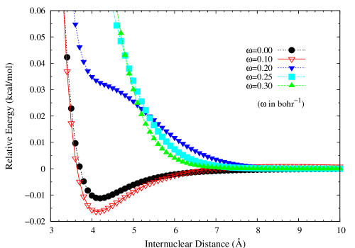
Figure 11: Potential energy curves for the lowest triplet states of H₂ associated with the short-range interparticle interactions $\text{erfc}(\omega r)/r$, calculated using the corresponding CCSD. The $\omega=0$ case is equivalent to the Coulomb interaction $1/r$.

References

• (1) A. J. Stone, The Theory of Intermolecular Forces, Clarendon Press, Oxford, 1996.
• (2) V. A. Parsegian, Van der Waals Forces: A Handbook for Biologists, Chemists, Engineers, and Physicists, Cambridge University Press, New York, 2006.
• (3) K. Lucas, Molecular Models for Fluids, Cambridge University Press, New York, 2007.
• (4) F. Jensen, Introduction to Computational Chemistry, Wiley, New York, 2007.
• (5) A. Salam, Molecular Quantum Electrodynamics: Long-Range Intermolecular Interactions, Wiley, Hoboken, NJ, 2010.
• (6) Y. S. Lee, Self-Assembly and Nanotechnology: A Force Balance Approach, Wiley, New York, 2008.
• (7) H. C. Hamaker, Physica, 1937, 4, 1058.
• (8) E. M. Lifshitz, Dokl. Akad. Nauk SSSR, 1954, 97, 643; 1955, 100, 879; E. M. Lifshitz, Zh. Eksp. Teor. Fiz., 1955, 29, 94 [Sov. Phys. JETP, 1956, 2, 73].
• (9) S.-W. Lee and W. M. Sigmund, Colloids Surf. A, 2002, 204, 43.
• (10) A. Milling, P. Mulvaney, and I. Larson, J. Colloid Interface Sci., 1996, 180, 460.
• (11) B. W. Ninham and V. A. Parsegian, J. Chem. Phys., 1970, 53, 3398.
• (12) L. Bergström, Adv. Colloid Interface Sci., 1997, 70, 125.
• (13) R. D. Adamson, J. P. Dombroski, and P. M. W. Gill, Chem. Phys. Lett., 1996, 254, 329.
• (14) R. D. Adamson and P. M. W. Gill, J. Mol. Struct. (Theochem), 1997, 398, 45.
• (15) S. F. Boys, Proc. R. Soc. London Ser. A, 1950, 200, 542.
• (16) P. M. W. Gill, Adv. Quantum Chem., 1994, 25, 141.
• (17) P. M. W. Gill and R. D. Adamson, Chem. Phys. Lett., 1996, 261, 105.
• (18) T. R. Adams, R. D. Adamson, and P. M. W. Gill, J. Chem. Phys., 1997, 107, 124.
• (19) J. Toulouse, F. Colonna, and A. Savin, Phys. Rev. A, 2004, 70, 062505.
• (20) A. D. Dutoi and M. Head-Gordon, J. Phys. Chem. A, 2008, 112, 2110.
• (21) J.-D. Chai and M. Head-Gordon, Chem. Phys. Lett., 2008, 467, 176.
• (22) J. A. Parkhill, J.-D. Chai, A. D. Dutoi, and M. Head-Gordon, Chem. Phys. Lett., 2009, 478, 283.
• (23) P. M. W. Gill, 2013, private communication.
• (24) P. Hohenberg and W. Kohn, Phys. Rev., 1964, 136, B864; W. Kohn and L. J. Sham, Phys. Rev., 1965, 140, A1133.
• (25) S. Kümmel and L. Kronik, Rev. Mod. Phys., 2008, 80, 3.
• (26) A. J. Cohen, P. Mori-Sánchez, and W. Yang, Chem. Rev., 2011, 112, 289.
• (27) P. M. W. Gill, R. D. Adamson, and J. A. Pople, Mol. Phys., 1996, 88, 1005.
• (28) P. A. M. Dirac, Proc. Cambridge Philos. Soc., 1930, 26, 376.
• (29) S. Paziani, S. Moroni, P. Gori-Giorgi, and G. B. Bachelet, Phys. Rev. B, 2006, 73, 155111.
• (30) J. P. Perdew and Y. Wang, Phys. Rev. B, 1992, 45, 13244.
• (31) J. P. Perdew, K. Burke, and M. Ernzerhof, Phys. Rev. Lett., 1996, 77, 3865.
• (32) E. Goll, H.-J. Werner, and H. Stoll, Phys. Chem. Chem. Phys., 2005, 7, 3917; E. Goll, H.-J. Werner, H. Stoll, T. Leininger, P. Gori-Giorgi, and A. Savin, Chem. Phys., 2006, 329, 276; E. Goll, H.-J. Werner, and H. Stoll, Chem. Phys., 2008, 346, 257.
• (33) Y. Shao, Z. Gan, E. Epifanovsky, A. T. B. Gilbert, M. Wormit, J. Kussmann, A. W. Lange, A. Behn, J. Deng, X. Feng, D. Ghosh, M. Goldey, P. R. Horn, L. D. Jacobson, I. Kaliman, R. Z. Khaliullin, T. Kuś, A. Landau, J. Liu, E. I. Proynov, Y. M. Rhee, R. M. Richard, M. A. Rohrdanz, R. P. Steele, E. J. Sundstrom, H. L. Woodcock III, P. M. Zimmerman, D. Zuev, B. Albrecht, E. Alguire, B. Austin, G. J. O. Beran, Y. A. Bernard, E. Berquist, K. Brandhorst, K. B. Bravaya, S. T. Brown, D. Casanova, C.-M. Chang, Y. Chen, S. H. Chien, K. D. Closser, D. L. Crittenden, M. Diedenhofen, R. A. DiStasio Jr., H. Do, A. D. Dutoi, R. G. Edgar, S. Fatehi, L. Fusti-Molnar, A. Ghysels, A. Golubeva-Zadorozhnaya, J. Gomes, M. W. D. Hanson-Heine, P. H. P. Harbach, A. W. Hauser, E. G. Hohenstein, Z. C. Holden, T.-C. Jagau, H. Ji, B. Kaduk, K. Khistyaev, J. Kim, J. Kim, R. A. King, P. Klunzinger, D. Kosenkov, T. Kowalczyk, C. M. Krauter, K. U. Lao, A. Laurent, K. V. Lawler, S. V. Levchenko, C. Y. Lin, F. Liu, E. Livshits, R. C. Lochan, A. Luenser, P. Manohar, S. F. Manzer, S.-P. Mao, N. Mardirossian, A. V. Marenich, S. A. Maurer, N. J. Mayhall, E. Neuscamman, C. M. Oana, R. Olivares-Amaya, D. P. O’Neill, J. A. Parkhill, T. M. Perrine, R. Peverati, A. Prociuk, D. R. Rehn, E. Rosta, N. J. Russ, S. M. Sharada, S. Sharma, D. W. Small, A. Sodt, T. Stein, D. Stück, Y.-C. Su, A. J. W. Thom, T. Tsuchimochi, V. Vanovschi, L. Vogt, O. Vydrov, T. Wang, M. A. Watson, J. Wenzel, A. White, C. F. Williams, J. Yang, S. Yeganeh, S. R. Yost, Z.-Q. You, I. Y. Zhang, X. Zhang, Y. Zhao, B. R. Brooks, G. K. L. Chan, D. M. Chipman, C. J. Cramer, W. A. Goddard III, M. S. Gordon, W. J. Hehre, A. Klamt, H. F. Schaefer III, M. W. Schmidt, C. D. Sherrill, D. G. Truhlar, A. Warshel, X. Xu, A. Aspuru-Guzik, R. Baer, A. T. Bell, N. A. Besley, J.-D. Chai, A. Dreuw, B. D. Dunietz, T. R. Furlani, S. R. Gwaltney, C.-P. Hsu, Y. Jung, J. Kong, D. S. Lambrecht, W. Z. Liang, C. Ochsenfeld, V. A. Rassolov, L. V. Slipchenko, J. E. Subotnik, T. Van Voorhis, J. M. Herbert, A. I. Krylov, P. M. W. Gill, and M. Head-Gordon, Mol. Phys., 2015, 113, 184.
• (34) T. H. Dunning, Jr., J. Chem. Phys., 1989, 90, 1007; D. E. Woon and T. H. Dunning, Jr., J. Chem. Phys., 1994, 100, 2975.
• (35) C. W. Murray, N. C. Handy, and G. J. Laming, Mol. Phys., 1993, 78, 997.
• (36) V. I. Lebedev and D. N. Laikov, Dokl. Math., 1999, 59, 477.
• (37) S. F. Boys and F. Bernardi, Mol. Phys., 1970, 19, 553.
• (38) M. Dion, H. Rydberg, E. Schröder, D. C. Langreth, and B. I. Lundqvist, Phys. Rev. Lett., 2004, 92, 246401.
• (39) A. Ruzsinszky, J. P. Perdew, and G. I. Csonka, J. Phys. Chem. A, 2005, 109, 11015.
• (40) J. P. Perdew, A. Ruzsinszky, G. I. Csonka, L. A. Constantin, and J. Sun, Phys. Rev. Lett., 2009, 103, 026403.
• (41) J. F. Dobson, K. McLennan, A. Rubio, J. Wang, T. Gould, H. M. Le, and B. P. Dinte, Aust. J. Chem., 2001, 54, 513.
• (42) A. D. Becke, J. Chem. Phys., 1993, 98, 5648.
• (43) S. Grimme, J. Chem. Phys., 2006, 124, 034108.
• (44) O. Gritsenko and E. J. Baerends, J. Chem. Phys., 2006, 124, 054115.
• (45) A. Savin, in Recent Developments and Applications of Modern Density Functional Theory, edited by J. M. Seminario, Elsevier, Amsterdam, 1996, pp. 327-357.
• (46) H. Iikura, T. Tsuneda, T. Yanai, and K. Hirao, J. Chem. Phys., 2001, 115, 3540.
• (47) T. Yanai, D. P. Tew, and N. C. Handy, Chem. Phys. Lett., 2004, 393, 51.
• (48) O. A. Vydrov, J. Heyd, A. V. Krukau, and G. E. Scuseria, J. Chem. Phys., 2006, 125, 074106.
• (49) E. Livshits and R. Baer, Phys. Chem. Chem. Phys., 2007, 9, 2932.
• (50) J.-D. Chai and M. Head-Gordon, J. Chem. Phys., 2008, 128, 084106.
• (51) J.-D. Chai and M. Head-Gordon, Phys. Chem. Chem. Phys., 2008, 10, 6615.
• (52) M. A. Rohrdanz and J. M. Herbert, J. Chem. Phys., 2008, 129, 034107.
• (53) J.-D. Chai and M. Head-Gordon, J. Chem. Phys., 2009, 131, 174105.
• (54) R. Peverati and D. G. Truhlar, J. Phys. Chem. Lett., 2011, 2, 2810.
• (55) Y.-S. Lin, C.-W. Tsai, G.-D. Li, and J.-D. Chai, J. Chem. Phys., 2012, 136, 154109.
• (56) Y.-S. Lin, G.-D. Li, S.-P. Mao, and J.-D. Chai, J. Chem. Theory Comput., 2013, 9, 263.
• (57) C.-W. Tsai, Y.-C. Su, G.-D. Li, and J.-D. Chai, Phys. Chem. Chem. Phys., 2013, 15, 8352.
• (58) J.-C. Lee, J.-D. Chai, and S.-T. Lin, RSC Adv., 2015, 5, 101370.
• (59) M. Levy, J. P. Perdew, and V. Sahni, Phys. Rev. A, 1984, 30, 2745.
• (60) C.-O. Almbladh and U. von Barth, Phys. Rev. B, 1985, 31, 3231.
• (61) R. van Leeuwen and E. J. Baerends, Phys. Rev. A, 1994, 49, 2421.
• (62) A. Görling, Phys. Rev. Lett., 1999, 83, 5459.
• (63) P. W. Ayers and M. Levy, J. Chem. Phys., 2001, 115, 4438.
• (64) A. P. Gaiduk and V. N. Staroverov, J. Chem. Phys., 2009, 131, 044107.
• (65) A. P. Gaiduk, D. S. Firaha, and V. N. Staroverov, Phys. Rev. Lett., 2012, 108, 253005.
• (66) C.-R. Pan, P.-T. Fang, and J.-D. Chai, Phys. Rev. A, 2013, 87, 052510.
• (67) J. P. Perdew and A. Zunger, Phys. Rev. B, 1981, 23, 5048.
• (68) T. Bally and G. N. Sastry, J. Phys. Chem. A, 1997, 101, 7923.
• (69) J. P. Perdew and M. Levy, Phys. Rev. Lett., 1983, 51, 1884.
• (70) L. J. Sham and M. Schlüter, Phys. Rev. Lett., 1983, 51, 1888.
• (71) L. J. Sham and M. Schlüter, Phys. Rev. B, 1985, 32, 3883.
• (72) G. K.-L. Chan, J. Chem. Phys., 1999, 110, 4710.
• (73) M. Grüning, A. Marini, and A. Rubio, J. Chem. Phys., 2006, 124, 154108.
• (74) E. Sagvolden and J. P. Perdew, Phys. Rev. A, 2008, 77, 012517.
• (75) A. J. Cohen, P. Mori-Sánchez, and W. Yang, Phys. Rev. B, 2008, 77, 115123.
• (76) P. Mori-Sánchez, A. J. Cohen, and W. Yang, Phys. Rev. Lett., 2008, 100, 146401.
• (77) P. Mori-Sánchez, A. J. Cohen, and W. Yang, Phys. Rev. Lett., 2009, 102, 066403.
• (78) T. Tsuneda, J.-W. Song, S. Suzuki, and K. Hirao, J. Chem. Phys., 2010, 133, 174101.
• (79) T. Stein, H. Eisenberg, L. Kronik, and R. Baer, Phys. Rev. Lett., 2010, 105, 266802.
• (80) X. Andrade and A. Aspuru-Guzik, Phys. Rev. Lett., 2011, 107, 183002.
• (81) W. Yang, A. J. Cohen, and P. Mori-Sánchez, J. Chem. Phys., 2012, 136, 204111.
• (82) J.-D. Chai and P.-T. Chen, Phys. Rev. Lett., 2013, 110, 033002.
• (83) A. Dreuw, J. L. Weisman, and M. Head-Gordon, J. Chem. Phys., 2003, 119, 2943.
• (84) D. J. Tozer, J. Chem. Phys., 2003, 119, 12697.
• (85) O. Gritsenko and E. J. Baerends, J. Chem. Phys., 2004, 121, 655.
• (86) A. Dreuw and M. Head-Gordon, J. Am. Chem. Soc., 2004, 126, 4007.
• (87) A. Dreuw and M. Head-Gordon, Chem. Rev., 2005, 105, 4009.
• (88) M. Hellgren and E. K. U. Gross, Phys. Rev. A, 2012, 85, 022514.
• (89) W.-T. Peng and J.-D. Chai, Phys. Chem. Chem. Phys., 2014, 16, 21564.
• (90) S. Grimme, J. Comput. Chem., 2004, 25, 1463.
• (91) S. Grimme, J. Comput. Chem., 2006, 27, 1787.
• (92) S. Grimme, J. Antony, S. Ehrlich, and H. Krieg, J. Chem. Phys., 2010, 132, 154104.
• (93) E. Brémond and C. Adamo, J. Chem. Phys., 2011, 135, 024106.
• (94) J.-D. Chai and S.-P. Mao, Chem. Phys. Lett., 2012, 538, 121.
• (95) K. Hui and J.-D. Chai, e-print arXiv:1510.00381.
• (96) P. Jankowski, B. Jeziorski, S. Rybak, and K. Szalewicz, J. Chem. Phys., 1990, 92, 7441.
• (97) H. L. Williams, K. Szalewicz, B. Jeziorski, R. Moszynski, and S. Rybak, J. Chem. Phys., 1993, 98, 1279.
• (98) B. Jeziorski, R. Moszynski, and K. Szalewicz, Chem. Rev., 1994, 94, 1887.
• (99) T. Korona, H. L. Williams, R. Bukowski, B. Jeziorski, and K. Szalewicz, J. Chem. Phys., 1997, 106, 5109.
• (100) E. M. Mas, K. Szalewicz, R. Bukowski, and B. Jeziorski, J. Chem. Phys., 1997, 107, 4207.
• (101) R. Bukowski, J. Sadlej, B. Jeziorski, P. Jankowski, K. Szalewicz, S. A. Kucharski, H. L. Williams, and B. M. Rice, J. Chem. Phys., 1999, 110, 3785.
• (102) M. Jeziorska, P. Jankowski, K. Szalewicz, and B. Jeziorski, J. Chem. Phys., 2000, 113, 2957.
• (103) M. Jeziorska, W. Cencek, K. Patkowski, B. Jeziorski, and K. Szalewicz, J. Chem. Phys., 2007, 127, 124303.
• (104) K. U. Lao and J. M. Herbert, J. Phys. Chem. A, 2012, 116, 3042.
• (105) A. Heßelmann and G. Jansen, Phys. Chem. Chem. Phys., 2003, 5, 5010.
• (106) A. J. Misquitta, R. Podeszwa, B. Jeziorski, and K. Szalewicz, J. Chem. Phys., 2005, 123, 214103.
• (107) A. Tekin and G. Jansen, Phys. Chem. Chem. Phys., 2007, 9, 1680.
• (108) K. Yu, J. G. McDaniel, and J. R. Schmidt, J. Phys. Chem. B, 2011, 115, 10054.
• (109) D. E. Taylor, F. Rob, B. M. Rice, R. Podeszwa, and K. Szalewicz, Phys. Chem. Chem. Phys., 2011, 13, 16629.
• (110) K. U. Lao and J. M. Herbert, J. Chem. Phys., 2014, 140, 044108.
• (111) G. Jansen, WIREs Comput. Mol. Sci., 2014, 4, 127.
• (112) J. P. Perdew, A. Ruzsinszky, L. A. Constantin, J. Sun, and G. I. Csonka, J. Chem. Theory Comput., 2009, 5, 902.
• (113) D. Peng, S. N. Steinmann, H. van Aggelen, and W. Yang, J. Chem. Phys., 2013, 139, 104112.
• (114) H. van Aggelen, Y. Yang, and W. Yang, Phys. Rev. A, 2013, 88, 030501(R).
• (115) J.-D. Chai, J. Chem. Phys., 2012, 136, 154104.
• (116) J.-D. Chai, J. Chem. Phys., 2014, 140, 18A521.
• (117) C.-S. Wu and J.-D. Chai, J. Chem. Theory Comput., 2015, 11, 2003.
• (118) D. J. Griffiths, Introduction to Quantum Mechanics, 2nd ed., Prentice Hall, Upper Saddle River, NJ, 2004.
• (119) See, for example, http://mathworld.wolfram.com/EinsteinSummation.html.
Refer to caption