Increasing relative nonclassicality quantified by standard entanglement potentials by dissipation and unbalanced beam splitting

Abstract

If a single-mode nonclassical light is combined with the vacuum on a beam splitter, then the output state is entangled. As proposed in [Phys. Rev. Lett. 94, 173602 (2005)], by measuring this output-state entanglement for a balanced lossless beam splitter, one can quantify the input-state nonclassicality. These measures of nonclassicality (referred to as entanglement potentials) can be based, in principle, on various entanglement measures, leading to the negativity (NP) and concurrence (CP) potentials, and the potential for the relative entropy of entanglement (REEP). We search for the maximal relative nonclassicality, which can be achieved by comparing two entanglement measures for (i) arbitrary two-qubit states and (ii) those which can be generated from a photon-number qubit via a balanced lossless beam splitter, where the qubit basis states are the vacuum and single-photon states. Surprisingly, we find that the maximal relative nonclassicality, measured by the REEP for a given value of the NP, can be increased (if NP$<$0.527) by using either a tunable beam splitter or by amplitude damping of the output state of the balanced beam splitter. We also show that the maximal relative nonclassicality, measured by the NP for a given value of the REEP, can be increased by phase damping (dephasing). Note that the entanglement itself is not increased by these losses (since they act locally), but the possible ratios of different measures are affected. Moreover, we show that partially-dephased states can be more nonclassical than both pure states and completely-dephased states, by comparing the NP for a given value of the REEP. Thus, one can conclude that not all standard entanglement measures can be used as entanglement potentials. Alternatively, one can infer that a single balanced lossless beam splitter is not always transferring the whole nonclassicality of its input state into the entanglement of its output modes. The application of a lossy beam splitter can solve this problem at least for the cases analyzed in this paper.

I Introduction

Nonclassical light plays a central role in quantum optics VogelBook ; PerinaBook and atom optics HarocheBook leading to various applications in quantum technologies, including quantum cryptography and communication, and optical quantum information processing KokBook .

In a sense, all states of light are quantum, so which of them can be considered classical? It is usually assumed that coherent states are classical. Thus, also their mixtures (e.g., thermal states) are classical. All other states of light are considered nonclassical (or quantum). Formally, this criterion can be given in terms of the Glauber-Sudarshan $P$ function Glauber63 ; Sudarshan63 : A given state $\sigma$ is nonclassical if and only if it is not described by a positive (semidefinite) function $P(\sigma)$. Thus, all finite superpositions (except for the vacuum) of arbitrary Fock states are nonclassical. We note that this definition “hides some serious problems”, as discussed in, e.g., Ref. Wunsche04 .

Various methods and criteria have been devised to test whether a given state of light is nonclassical (see, e.g., Refs. VogelBook ; DodonovBook ; PerinaBook ; Miran10 ; Bartkowiak11 ). However, with respect to the above definition, it seems much more interesting physically to quantify the nonclassicality of light rather than only to test (detect) it. For the last thirty years various measures of nonclassicality have been studied (for reviews see Refs. DodonovBook ; VogelBook ). The most popular of them include entanglement potentials, nonclassical distance Hillery87 , and nonclassical depth Lee91 ; Lutkenhaus95 . For a comparative studies of these measures see recent Refs. Miran15 ; Arkhipov15 and references therein. Other measures or parameters of nonclassicality were described in, e.g., the recent Refs. Mari11 ; Gehrke12 ; Nakano13 ; Meznaric13 . Many studies have been devoted to the nonclassical volume Kenfack04 , which is the volume of the negative part of the Wigner function of a given state. But it should be stressed that this nonclassical volume is not a good measure but only a parameter of nonclassicality, as it vanishes for some nonclassical states, including ideal squeezed states.

In this paper we solely analyze universal nonclassicality measures defined via entanglement potentials, which are closely related to standard entanglement measures. Specifically, as introduced by Asboth et al. Asboth05 , one can quantify the nonclassicality of a given single-mode state by measuring the entanglement generated from this state and the vacuum by an auxiliary balanced beam splitter (BS). This approach is operationally much simpler than other nonclassicality measures, including the mentioned nonclassical depth and distance.

To be more specific, the nonclassicality of a single-mode state $\sigma$ can be quantified, according to Ref. Asboth05 , by the entanglement of the output state $\rho_{\rm out}$ of an auxiliary lossless balanced BS with the state $\sigma$ and the vacuum $|0\rangle$ at the inputs, i.e.,

$$\rho_{\rm out}=U_{\rm BS}(\sigma\otimes\mbox{$|0\rangle$}\mbox{$\langle 0|$})U^{\dagger}_{\rm BS},$$ (1)

where $U_{\rm BS}=\exp(-iH\theta)$, with $\hbar=1$ and $\theta=\pi/2$, is the unitary transformation for a balanced BS, which can be given in terms of the Hamiltonian $H=\frac{1}{2}i(a_{1}^{\dagger}a_{2}-a_{1}a_{2}^{\dagger}),$ where $a_{1,2}$ ($a_{1,2}^{\dagger}$) are the annihilation (creation) operators of the input modes. This transformation $U_{\rm BS}$ is equivalent to that applied in Ref. Miran15 up to a local unitary transformation, which does not change the entanglement of $\rho_{\rm out}$, as quantified by any “good” entanglement measure. Note that linear transformations (like that performed by a BS) do not change the nonclassicality of a given state. The output state $\rho_{\rm out}$ is entangled if and only if the input state $\sigma$ is nonclassical. In particular, for the input in an arbitrary finite-dimensional state, except for the vacuum state, the output state is entangled. It should be stressed that the standard entanglement potentials, as proposed (and numerically verified) in Ref. Asboth05 , are based solely on the special case of $\rho_{\rm out}$ for $\theta=\pi/2$, i.e., when the BS transmissivity is equal to 1/2 corresponding to a balanced (50/50) BS.

In this paper, we compare three standard entanglement potentials of a single-qubit input state $\sigma$ corresponding to the entanglement measures of the two-qubit output state $\rho_{\rm out}$. The analyzed qubit is assumed to be in an arbitrary (coherent or incoherent) superposition of the vacuum and single-photon Fock states, so it can be referred to as a photon-number qubit. We quantify the nonclassicality of $\sigma$ by the negativity potential (NP), concurrence potential (CP), and the potential for the relative entropy of entanglement (REEP):

$${\rm NP}(\sigma) = N(\rho_{\rm out}),$$ (2)

$${\rm CP}(\sigma) = C(\rho_{\rm out}),$$ (3)

$${\rm REEP}(\sigma) = E_{R}(\rho_{\rm out}),$$ (4)

which are defined via the negativity $N$, concurrence $C$, and REE $E_{R}$ for $\rho_{\rm out}$. Although these entanglement measures are well-known, for clarity, we give their definitions and operational interpretations in Appendix A. The REEP is also referred to as the entropic entanglement potential in the original Ref. Asboth05 . We emphasize again that we refer to entanglement potential of a given state $\sigma$ for any entanglement measure applied to the output $\rho_{\rm out}$.

Various entanglement potentials, which are based on this unified approach of measuring nonclassicality and entanglement, have been attracting increasing interest especially during the past year (see, e.g., Refs. Vogel14 ; Mraz14 ; Miran15 ; Tasgin15 ; Killoran15 ; Ge15 ). The ultimate goal of such studies is to demonstrate how nonclassicality can operationally be used as a resource for quantum technologies and quantum information processing. Thus, one of the most natural and fundamental questions in this area addresses the relationship between entanglement and other types of nonclassicality. For example, the problem of faithfully converting single-system nonclassicality into entanglement in general mathematical terms was addressed in Ref. Killoran15 with the following conclusions: “These results generalize and link convertibility properties from the resource theory of coherence, spin coherent states, and optical coherent states, while also revealing important connections between local and non-local quantum correlations.” A conservation relation of nonclassicality and entanglement in a balanced beam splitter was found for some limited classes of Gaussian states in Ref. Ge15 . A related single-mode nonclassicality measure based on the Simon-Peres-Horodecki criterion was described for Gaussian states in Ref. Tasgin15 . Refs. Vogel14 ; Mraz14 demonstrated that the rank of the two-mode entanglement of a single-mode state $\sigma$ is equal to the rank of the expansion of $\sigma$ in terms of classical coherent states. It was shown in Ref. Miran15 that the CP of a single qubit state $\sigma$ can be interpreted as a Hillery-type nonclassical distance, defined by the Bures distance of $\sigma$ to the vacuum, which is the closest classical state in the single-qubit Hilbert space. Moreover, it is known that the statistical mixtures of the vacuum and single-photon states can be more nonclassical than their superpositions, as shown in Ref. Miran15 by comparing the NP and CP.

Here we present a comparative study of these three entanglement potentials, to show that such quantified relative nonclassicality, i.e., the nonclassicality of one measure relative to another, can be increased by damping and unbalanced beam splitting. Moreover, in Ref. Miran15 we showed that both pure and completely-dephased single-qubit states can be considered the most nonclassical by comparing some nonclassicality measures. Here we show that also some partially-dephased states can be the most relatively nonclassical in terms of the highest negativity potential for a given value of the REE potential.

The paper is organized as follows. In Sec. II, we calculate the entanglement potentials for single-qubit states. In Sec. III, we find the most nonclassical single-qubit states via the standard entanglement potentials. In this section and also in Sec. IV, we show that there are two-qubit states, which are more entangled than those which can be generated from a single-qubit state and the vacuum by a balanced lossless BS. In Sec. V, we show that by applying a tunable and/or lossy BS, we can generate relative entanglement higher than that in the standard approach. We refer to this modified approach as being based on generalized entanglement potentials. Moreover, for the completeness and clarity of our presentation, we recall known results in appendices, including definitions of the standard entanglement measures and boundary states for arbitrary two-qubit states. We conclude in Sec. VI.

II Entanglement potentials for single-qubit states

To make our presentation simple and convincing, we analyze, as in Ref. Miran15 , the nonclassicality of only single-qubit states:

$$\sigma(p,x)=\sum_{m,n=0}^{1}\sigma_{mn}\mbox{$|m\rangle$}\mbox{$\langle n|$}=\left[\begin{array}[]{cc}1-p&x\\ x^{*}&p\end{array}\right],$$ (5)

which are spanned by the vacuum $|0\rangle$ and the single-photon Fock state $|1\rangle$. Here $p\in[0,1]$ is the mixing parameter, and $|x|\in[0,\sqrt{p(1-p)}]$, which is often interpreted as a coherence parameter. Analogously, in the context of the NMR spectroscopy of a spin qubit, $x$ and $x^{*}$ are called the coherences between the states $|0\rangle$ and $|1\rangle$ LevittBook . The relation between the coherence and entanglement of a partially coherent state of light was recently studied in Ref. Svozilik15 . An experimental demonstration of the nonclassicality of the optical qubit states, given in Eq. (5), was reported in Ref. Lvovsky02 based on the nonclassicality criterion of Vogel VogelBook . Note that the only classical state of $\sigma(p,x)$ is for $p=0$, corresponding to the vacuum. Equation (1) for $\sigma(p,x)$ simplifies to

$$\rho_{\rm out}(p,x)=\left[\begin{array}[]{cccc}1-p&-\frac{1}{\sqrt{2}}x&\frac{1}{\sqrt{2}}x&0\\ -\frac{1}{\sqrt{2}}x^{*}&\frac{1}{2}p&-\frac{1}{2}p&0\\ \frac{1}{\sqrt{2}}x^{*}&-\frac{1}{2}p&\frac{1}{2}p&0\\ 0&0&0&0\\ \end{array}\right].$$ (6)

Here we study how well the entanglement potentials can serve as measures of nonclassicality for a balanced BS.

As shown in Ref. Miran15 , the concurrence potential is given by a simple formula

$${\rm CP}[\sigma(p,x)]=p,$$ (7)

for the arbitrary state given in Eq. (5). Note that this potential is independent of the coherence parameter $x$. Surprisingly, the negativity potential is given by a much more complicated formula

$${\rm NP}[\sigma(p,x)]=\frac{1}{3}\left[2{\rm Re}\left(\sqrt[3]{2\sqrt{\alpha_{1}}+2\alpha_{2}}\right)+p-2\right],$$ (8)

for a general state $\sigma(p,x)$, where $\alpha_{1}$ ($\alpha_{2}$) is a polynomial of the 6th (3rd) order in $p$ and the 6th (2nd) order in $|x|$, as explicitly given in Ref. Miran15 . Obviously, Eq. (8) simplifies considerably for special states, including those studied in the next sections. Equation (8) can be obtained from the formula valid for an arbitrary two-qubit state $\rho$ Bartkiewicz15 :

$$48D+3N^{4}+6N^{3}-6N^{2}\Pi^{\prime}_{2}-4N(3\Pi^{\prime}_{2}-2\Pi^{\prime}_{3})=0,$$ (9)

expressing the negativity via the invariant moments $\Pi^{\prime}_{n}=\Pi_{n}-1={\rm Tr}[(\rho^{\Gamma})^{n}]-1$ and the determinant $D=\det\rho^{\Gamma}$, where $\rho^{\Gamma}$ denotes the partially transposed $\rho$. These moments are directly measurable, as shown in Refs. Bartkiewicz15b . This general formula simplifies for the special two-qubit states $\rho=\rho_{\rm out}$, which are generated by a balanced BS. Thus, we can simply express the coherence parameter $|x|$ as a function of the negativity (or negativity potential) and the mixing parameter $p$ as follows:

$$|x|=f(p,N)=\tfrac{1}{2}\sqrt{(1+p/N)[2N(N+1)-(N+p)^{2}]}$$ (10)

for any $p\in[N,\sqrt{2N(N+1)}-N]$. Thus, an arbitrary single qubit state $\sigma(p,x)$ can be given as

$$\sigma^{\prime}(p,N,\phi) \equiv \sigma[p,x=f(p,N)\exp(i\phi)],$$ (11)

where $\phi={\rm Arg}(x)$ is the phase factor of the coherence parameter $x$. In the context of our nonclassicality analysis, the inclusion of $\phi$ in Eqs. (5) and (11) is actually irrelevant, as any “good” nonclassicality measures (including the entanglement potentials) do not depend on $\phi$. Thus, for simplicity, we can set $\phi=0$.

The calculation of the REE potential is even more demanding as explained in Appendix A. We have calculated the REE analytically only for some special states, including pure and completely-dephased single-qubit states, and the completely-dephased output states of a BS. In other cases, the REE potential is calculated only numerically based on semidefinite algorithm implemented in Ref. Girard15 .

III Most relatively nonclassical single-qubit states via entanglement potentials

Here we address the following question: which single-qubit states are the most nonclassical if quantified by one entanglement potential relative to another. Specifically, we compare the nonclassicality of states for a given entanglement potential assuming that the states have the same nonclassicality in terms of another entanglement potential.

Figure 1 shows such comparison of the three entanglement potentials for randomly generated single-qubit states $\sigma$. These graphs are obtained as follows: For a given $\sigma$, we calculated the potentials ${\rm NP}(\sigma)$, ${\rm CP}(\sigma)$, and ${\rm REEP}(\sigma)$, and then plotted a point at $[{\rm NP}(\sigma),{\rm CP}(\sigma)]$ in Fig. 1(a), another point at $[{\rm REEP}(\sigma),{\rm CP}(\sigma)]$ in Fig. 1(b), and $[{\rm REEP}(\sigma),{\rm NP}(\sigma)]$ in Fig. 1(c). The Monte-Carlo simulated points occupy limited areas. Now we discuss the states on their boundaries. Note that the red curves in Fig. 1 show the boundaries of the entanglement of arbitrary two-qubit states $\rho$ (see Appendix B), instead of $\rho_{\rm out}$ only. Figure 2 shows more explicitly that there is a two-qubit entanglement (corresponding to the red regions), which cannot be generated from single-qubit states and the vacuum by a balanced lossless BS.

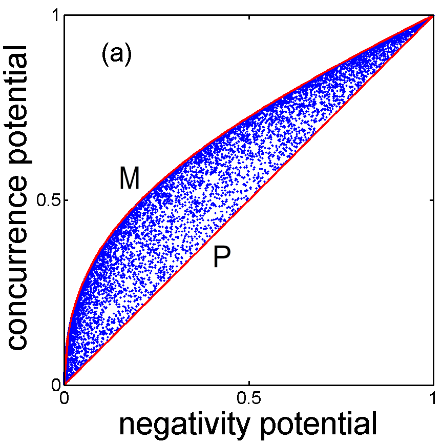
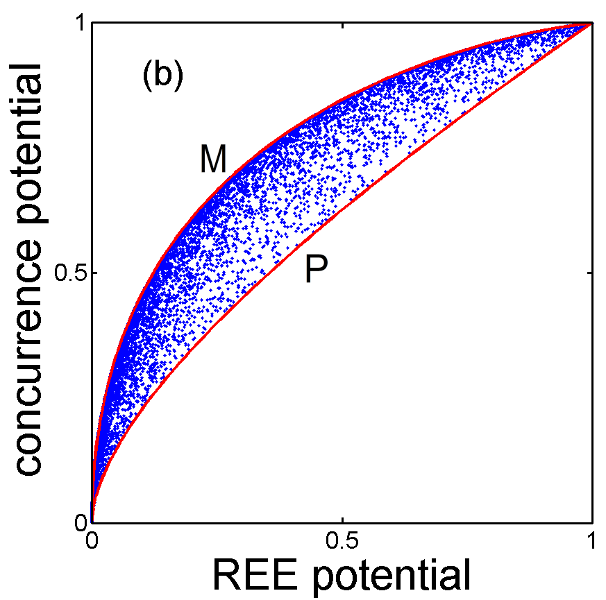
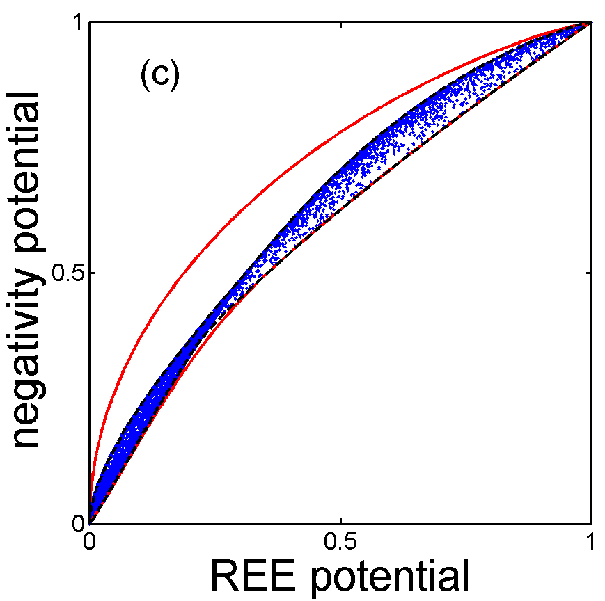
Figure 1: (Color online) Entanglement potentials for 15,000 single-qubit states $\sigma$ generated via a Monte Carlo simulation. These entanglement potentials correspond to the entanglement measures for the two-qubit states $\rho_{\rm out}$ generated from $\sigma$ by a balanced beam splitter. The solid red curves show the boundaries of the allowed entanglement for arbitrary two-qubit states $\rho$ (discussed in Appendix B). Note that the simulated states $\rho_{\rm out}$ lie in the area bounded by the solid red curves for the concurrence potential for given values of both (a) the negativity potential and (b) the potential of the relative entropy of entanglement (REE). This is not the case for (c) the negativity potential for a given value of the REE potential, as the states $\rho_{\rm out}$ lie in the area, bounded by the dashed black curves, which is smaller than the area covered by the states $\rho$. The upper (lower) red curves in panels (a) and (b) correspond to the completely-dephased states ${\sigma_{\rm M}}$ (pure states ${\sigma_{\rm P}}$) as compactly indicated by M (P). The meaning of the red and black curves in panel (c) is more detailed, as shown in Fig. 3.

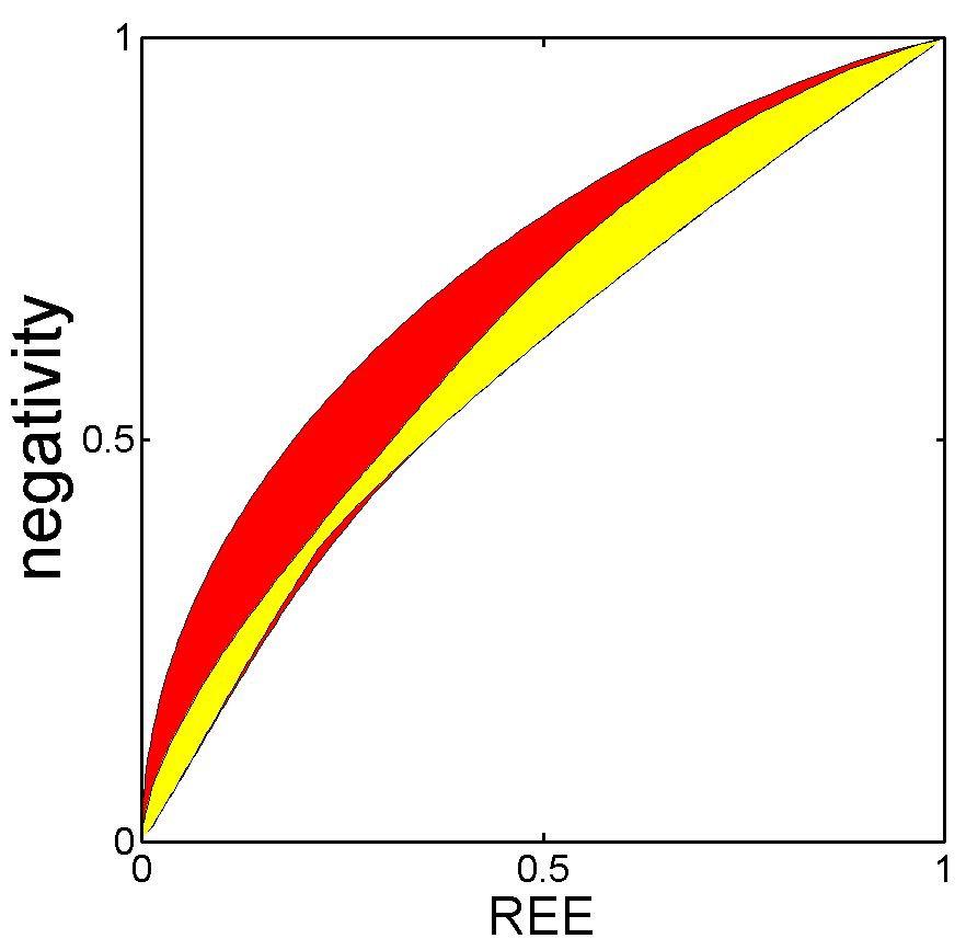
Figure 2: (Color online) Allowed values of the negativity for a given value of the REE for the states $\rho_{\rm out}$, defined in Eq. (1), generated from arbitrary single-qubit states (in yellow regions), and those for arbitrary two-qubit states $\rho$ (in red and yellow regions). The main goal of this paper is to show how the entanglement, corresponding to any point in the red regions, can be generated from a single-qubit state.

III.1 When pure states are maximally nonclassical

The most general single-qubit pure state is given by

$$\mbox{$|\psi\rangle$}=\sqrt{1-p}\mbox{$|0\rangle$}+e^{i\phi}\sqrt{p}\mbox{$|1\rangle$},$$ (12)

up to an irrelevant global phase. So, ${\sigma_{\rm P}}\equiv\mbox{$|\psi\rangle$}\mbox{$\langle\psi|$}$ is a special case of Eq. (5) for $|x|=\sqrt{p(1-p)}$ and $\phi={\rm Arg(}x)$. As already mentioned, the nonclassicality measures are insensitive to the relative phase $\phi$, so we can set $\phi=0$. The entanglement potentials for a pure state ${\sigma_{\rm P}}$ are simply given by:

$${\rm CP}({\sigma_{\rm P}}) = {\rm NP}({\sigma_{\rm P}})=p,$$ (13)

$${\rm REEP}({\sigma_{\rm P}}) = h\left(\textstyle{\frac{1}{2}}[1+\sqrt{1-p^{2}}]\right),$$ (14)

where $h(y)=-y\log_{2}y-(1-y)\log_{2}(1-y)$ is the binary entropy. For clarity, we recall the well-known property that ${\rm REEP}({\sigma_{\rm P}})$ is equal to the entanglement of formation $E_{F}({\rho_{\rm P}})$ and to the von Neumann entropy of a reduced density matrix, say, ${\rm Tr}_{1}({\rho_{\rm P}})$.

We find that pure states are the most nonclassical single-qubit states in terms of: (i) the maximal NP for a given value of ${\rm CP}\in[0,1]$ [see Fig. 1(a)], (ii) the maximal REEP for a given value of ${\rm CP}\in[0,1]$ [see Fig. 1(b)], and (iii) the maximal REEP for a given value of ${\rm NP}\in[N_{2},1]$, where $N_{2}\approx 0.527$ [see Figs. 1(c), 2 and 3]. These results are summarized in Table I. Note that pure states are very close to maximal nonclassical states concerning the largest NP for a given ${\rm REEP}\lesssim 0.1$ [see Fig. 3].

Table 1: Maximally-nonclassical states (MNS) of a single-qubit state $\sigma$, maximally-entangled states (MES) $\rho_{\rm out}$ (generated by a lossless balance BS), and maximally-entangled states $\rho$ (generated by any method) according to one entanglement measure (or entanglement potential) for a given value of another entanglement measure (or entanglement potential). The extra resources enable to increase the entanglement of $\rho_{\rm out}$ (so, also the nonclassicality of $\sigma).$ These include the amplitude-damping channel (ADC), phase-damping channel (PDC), and tunable beam splitter (TBS). Notation: CP is the concurrence potential, NP is the negativity potential, REEP is the potential of the relative entropy of entanglement. The special values of $N_{i}$ and $E_{i}$ are defined in Fig. 3. The output extremal states read: ${\rho_{\rm B}}$ are the Bell-diagonal states, ${\rho_{\rm P}}$ are pure states, ${\rho_{\rm H}}$ are the Horodecki states corresponding to the completely-dephased single-qubit states ${\sigma_{\rm M}}$, ${\rho_{\rm Z}}$ are the two-qubit states generated from single-qubit optimally-dephased states ${\sigma_{\rm Z}}$, and ${\rho_{\rm A}}$ are the optimal generalized Horodecki states. This is a summary of all the cases, when the nonclassicality of $\sigma$, as quantified by the three standard entanglement potentials, can or cannot be increased.

Potential 1	for a given value	MNS	MES	MES	extra resources
	of Potential 2	$\sigma$	$\rho_{\rm out}$	$\rho$
CP	NP$\in[0,1]$	${\sigma_{\rm M}}$	${\rho_{\rm H}}$	${\rho_{\rm H}}$	—
CP	REEP$\in[0,1]$	${\sigma_{\rm M}}$	${\rho_{\rm H}}$	${\rho_{\rm H}}$	—
NP	CP$\in[0,1]$	${\sigma_{\rm P}}$	${\rho_{\rm P}}$	${\rho_{\rm P}}$	—
NP	REEP$\in[0,E_{3})$	${\sigma_{\rm Z}}$	${\rho_{\rm Z}}$	${\rho_{\rm B}}$	PDC
NP	REEP$\in[E_{3},1]$	${\sigma_{\rm M}}$	${\rho_{\rm H}}$	${\rho_{\rm B}}$	PDC
REEP	CP$\in[0,1]$	${\sigma_{\rm P}}$	${\rho_{\rm P}}$	${\rho_{\rm P}}$	—
REEP	NP$\in[0,N_{1})$	${\sigma_{\rm M}}$	${\rho_{\rm H}}$	${\rho_{\rm A}}$	ADC or TBS
REEP	NP$\in[N_{1},N_{2})$	${\sigma_{\rm P}}$	${\rho_{\rm P}}$	${\rho_{\rm A}}$	ADC or TBS
REEP	NP$\in[N_{2},1]$	${\sigma_{\rm P}}$	${\rho_{\rm P}}$	${\rho_{\rm P}}$	—

III.2 When completely-dephased states are maximally nonclassical

Now we consider the nonclassicality of a statistical mixture of the vacuum $|0\rangle$ and single-photon state $|1\rangle$. This is a special case of Eq. (5) for the vanishing coherence parameter $x=0$, i.e.,

$${\sigma_{\rm M}}=\sigma(p,x=0)=(1-p)\mbox{$|0\rangle$}\mbox{$\langle 0|$}+p\mbox{$|1\rangle$}\mbox{$\langle 1|$}.$$ (15)

These mixtures are referred here to as completely-dephased states, but can also be referred to as completely-mixed states Miran15 , or the Fock diagonal states, to emphasize that these states are diagonal in the Fock basis. As shown in Ref. Miran15 , these states can be considered the most nonclassical by comparing the CP for a given value of the NP. Here, we analyze the nonclassicality of ${\sigma_{\rm M}}$ also with respect to the REE potential.

First we recall that ${\sigma_{\rm M}}$ is transformed by the balanced BS (with the vacuum in the other port) into the Horodecki state

$${\rho_{\rm H}}(p)=\rho_{\rm out}(p,0)=p\mbox{$|\psi^{-}\rangle$}\mbox{$\langle\psi^{-}|$}+(1-p)\mbox{$|00\rangle$}\mbox{$\langle 00|$},$$ (16)

which is a mixture of a maximally-entangled state, here the singlet state $\mbox{$|\psi^{-}\rangle$}=(\mbox{$|10\rangle$}-\mbox{$|01\rangle$})/\sqrt{2}$, and a separable state (here, the vacuum) orthogonal to it. The entanglement properties of the Horodecki state were studied intensively (see Ref. Horodecki09review for a review), so we can instantly write the entanglement potentials for ${\sigma_{\rm M}}$ as:

$${\rm CP}({\sigma_{\rm M}}) = p,$$

$${\rm NP}({\sigma_{\rm M}}) = \sqrt{(1-p)^{2}+p^{2}}-(1-p),$$ (17)

$${\rm REEP}({\sigma_{\rm M}}) = (p-2)\log_{2}(1-p/2)+(1-p)\log_{2}(1-p).$$

Thus, the REE potential can easily be expressed as a function of the other potentials ${\rm NP}=N$ and ${\rm CP}=C$, as follows:

$${\rm REEP}[{\sigma_{\rm M}}(C)]={\rm REEP}[{\sigma_{\rm M}}(\sqrt{2N(1+N)}-N)].$$ (18)

We observe that the completely-dephased states ${\sigma_{\rm M}}$ are the most nonclassical single-qubit states concerning: (i) the maximal CP for a given value of ${\rm NP}\in[0,1]$ [see Fig. 1(a)], (ii) the maximal CP for a given value of ${\rm REEP}\in[0,1]$ [see Fig. 1(b)], (iii) the maximal NP for a given value of the REEP, $E\in[E_{3},1]$, where $E_{3}=0.397$ [see Fig. 3], and (iv) the maximal REEP for a given value of ${\rm NP}\in[0,N_{1}]$, where $N_{1}=0.377$. These results are also summarized in Table I.

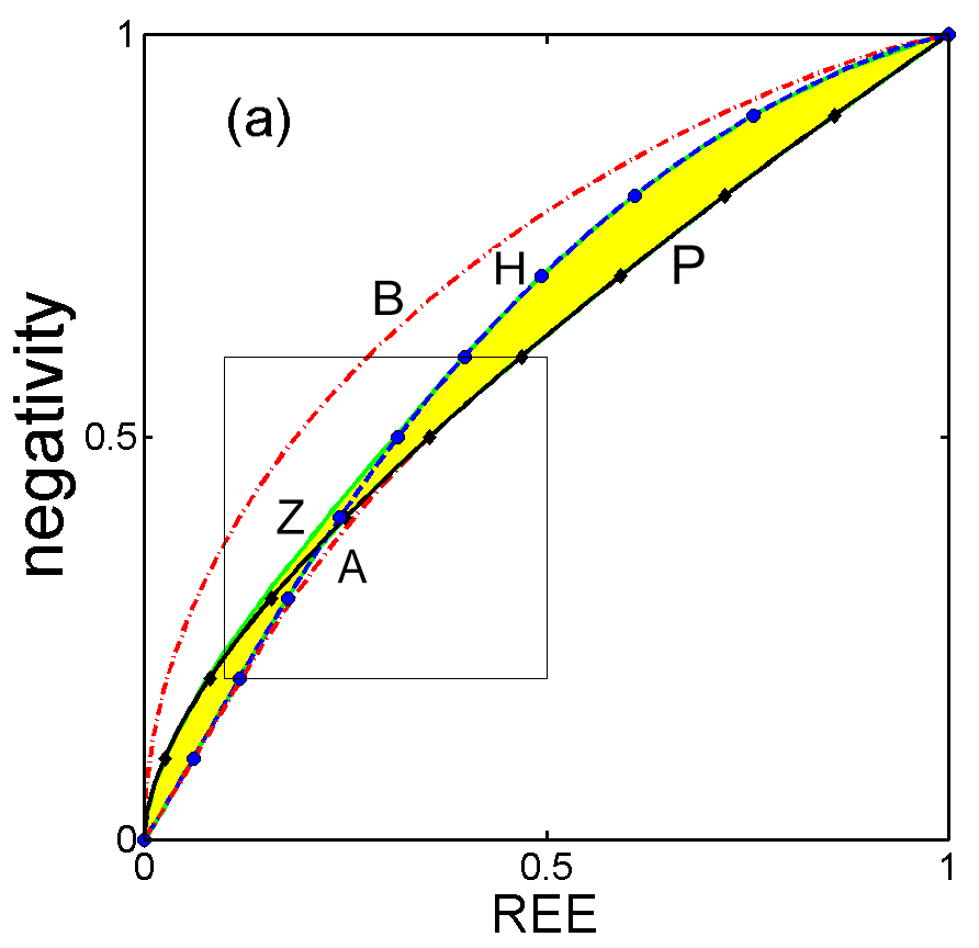
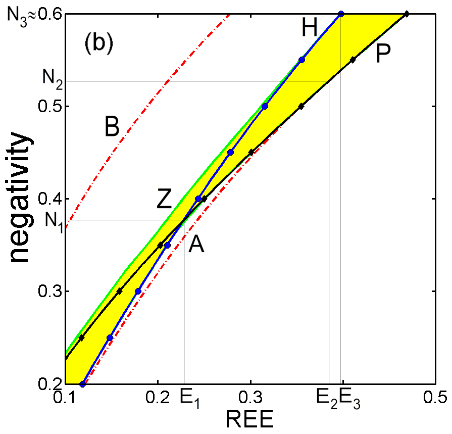
Figure 3: (Color online) (a) Boundary states and special points corresponding to Fig. 2. (b) The inset of panel (a) showing, in greater detail, the boundary states: ${\rho_{\rm B}}$ are the Bell-diagonal states (corresponding to the upper red dot-dashed curve), ${\rho_{\rm P}}$ (or equivalently ${\sigma_{\rm P}}$) are pure states (solid black curve with diamonds), ${\rho_{\rm H}}$ are the Horodecki states (solid blue curve with circles), which correspond to the single-qubit completely-dephased states ${\sigma_{\rm M}}$, ${\rho_{\rm A}}$ are the optimal generalized Horodecki states (lower red dot-dashed curve), and ${\rho_{\rm Z}}$ are the two-qubit states (green solid curve, which is the upper bound of the yellow region) generated from single-qubit optimally-dephased states ${\sigma_{\rm Z}}$. Special points are marked at: $(E_{1}\approx 0.228,N_{1}\approx 0.377)$, $(E_{2}\approx 0.385,N_{2}\approx 0.527)$, and $(E_{3}\approx 0.397,N_{3}\approx 0.6)$. Note that here, and in Fig. 2, we refer to entanglement measures rather than directly to the corresponding entanglement potentials, because some of the marked regions and curves cannot be reached by the states generated by the standard entanglement potentials.

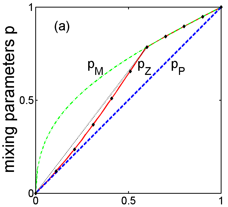
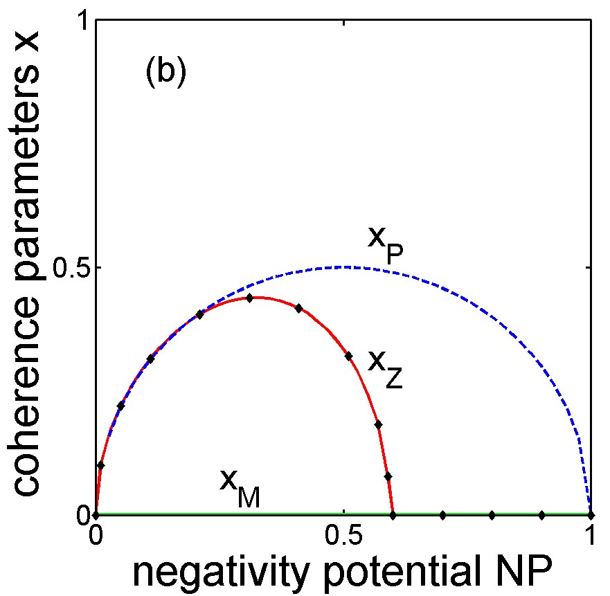
Figure 4: (Color online) Mixing and coherence parameters for the optimally-dephased state ${\sigma_{\rm Z}}=\sigma(p_{\rm Z},x_{\rm Z})$, completely-dephased state ${\sigma_{\rm M}}=\sigma(p_{\rm M},x_{\rm M}=0)$, and pure state ${\sigma_{\rm P}}=\sigma(p_{\rm P},x_{\rm P})$ as a function of their negativity potential $N={\rm NP}({\sigma_{\rm Z}})={\rm NP}({\sigma_{\rm M}})={\rm NP}({\sigma_{\rm P}})$. Dotted black line in panel (a) is added, to show that $p_{Z}$ does not linearly depend on $N\in[0,0.6]$. We recall that ${\sigma_{\rm Z}}$ exhibits the highest nonclassicality if considered the maximum negativity potential for a given value of the REEP.

III.3 When partially-dephased states are maximally nonclassical

A closer analysis of Fig. 3 shows that pure states and completely-dephased states do not have always the greatest entanglement potentials. Thus, let us define the following optimally-dephased states

$${\sigma_{\rm Z}}(N) = \sigma[p_{\rm opt},x_{\rm opt}=f(p_{\rm opt},N)],$$ (19)

$${\rho_{\rm Z}} \equiv U_{\rm BS}\big{(}{\sigma_{\rm Z}}\otimes\mbox{$|0\rangle$}\mbox{$\langle 0|$}\big{)}U^{\dagger}_{\rm BS},$$ (20)

which are the most nonclassical concerning the largest NP for a given value of the REEP. Here, $f$ is given in Eq. (10), $U_{\rm BS}$ is defined below Eq. (1), while the optimal mixing parameter $p_{\rm opt}\equiv p_{Z}$ is found numerically, as ${\rm REEP}\{\sigma[p_{\rm opt},f(p_{\rm opt},N)]\}=\min_{p}{\rm REEP}\{\sigma[p,f(p,N)]\}$, and shown in Fig. 4(a). Note that the optimal coherence parameter $x_{\rm opt}\equiv x_{Z}$, which is shown in Fig. 4(b), is simply given by $f(p_{\rm opt},N)$. We numerically found that ${\sigma_{\rm Z}}$ becomes ${\sigma_{\rm M}}$ for $N\geq N_{3}\approx 0.6$, as shown in Fig. 3. Thus, these partially-dephased states become completely dephased. Moreover, the ${\sigma_{\rm Z}}$ are very close to pure states ${\sigma_{\rm P}}$ for ${\rm NP}\lesssim 0.2$. The optimal states ${\sigma_{\rm Z}}$ are the most distinct from ${\sigma_{\rm P}}$ and ${\sigma_{\rm M}}$ for ${\rm NP}$ near $N_{1}$ [see Fig. 3(b)].

IV Special values of entanglement potentials

Here we analyze in detail three characteristic points shown in Fig. 3 corresponding to the negativity (or negativity potential) for a given value of the REE (or the REE potential).

Point 1: For the negativity potential $N_{1}\approx 0.377$ and the REE potential $E_{1}\approx 0.228$, it holds that pure and completely-dephased states have the same negativity and REE potentials, i.e.,

$${\rm NP}[{\sigma_{\rm P}}(N_{1})] = {\rm NP}[{\sigma_{\rm M}}(N_{1})]=N_{1},$$

$${\rm REEP}[{\sigma_{\rm P}}(N_{1})] = {\rm REEP}[{\sigma_{\rm M}}(N_{1})]=E_{1}.$$ (21)

Then one observes that

$${\rm NP}({\sigma_{\rm P}})>{\rm NP}({\sigma_{\rm M}}) {\rm for}\;0<{\rm REEP}<E_{1},$$

$${\rm NP}({\sigma_{\rm P}})<{\rm NP}({\sigma_{\rm M}}) {\rm for}\;E_{1}<{\rm REEP}<1.\quad$$ (22)

Point 2: For the negativity potential $N\geq N_{2}\approx 0.527$ corresponding to the REE potential $E\geq E_{2}\approx 0.385$, one finds that the optimal generalized Horodecki state ${\rho_{\rm A}}$, , defined in Eq. (50), which maximizes the REE for a given value of the negativity for arbitrary two-qubit states, becomes a two-qubit pure state ${\rho_{\rm P}}$ corresponding to a single-qubit pure state ${\sigma_{\rm P}}$, i.e.,

$${\rm NP}[{\sigma_{\rm P}}(N)] = N[{\rho_{\rm A}}(N)]=N,$$

$${\rm REEP}[{\sigma_{\rm P}}(N)] = E_{R}[{\rho_{\rm A}}(N)]=E,\quad\text{if}\;N\geq N_{2}.\quad$$ (23)

Point 3: For the negativity potential $N\geq N_{3}\approx 0.6$ and the REE potential $E\geq E_{3}\approx 0.397$, we find that the optimally-dephased state ${\sigma_{\rm Z}}$, which maximizes the negativity potential for a given value of the REE potential, becomes a completely-dephased state ${\sigma_{\rm M}}$, i.e.,

$${\rm NP}[{\sigma_{\rm M}}(N)] = {\rm NP}[{\sigma_{\rm Z}}(N)]=N,$$

$${\rm REEP}[{\sigma_{\rm M}}(N)] = {\rm REEP}[{\sigma_{\rm Z}}(N)]=E,\;\text{if}\;N\geq N_{3}.\quad\quad$$ (24)

Moreover, although it is not clear on the scale of Fig. 3, the optimally-dephased state ${\sigma_{\rm Z}}$ becomes exactly a pure state ${\sigma_{\rm P}}$ only for the vacuum and single-photon states, i.e.,

$${\rm NP}[{\sigma_{\rm P}}(N)] = {\rm NP}[{\sigma_{\rm Z}}(N)]=N,$$

$${\rm REEP}[{\sigma_{\rm P}}(N)] = {\rm REEP}[{\sigma_{\rm Z}}(N)]=E,\;\text{if}\;N=0,1.\quad\quad$$ (25)

Analogously, the optimal generalized Horodecki state ${\rho_{\rm A}}$ becomes exactly the standard Horodecki state ${\rho_{\rm H}}$, which can be generated from a completely-dephased state ${\sigma_{\rm M}}$, only for the same cases, as in Eq. (25), i.e.,

$$N[{\rho_{\rm H}}(N)] = N[{\rho_{\rm A}}(N)]=N,$$

$$E_{R}[{\rho_{\rm H}}(N)] = E_{R}[{\rho_{\rm A}}(N)]=E,\quad\text{if}\;N=0,1.\quad$$ (26)

Nevertheless, ${\rho_{\rm H}}$ is a good approximation of ${\rho_{\rm A}}$, and ${\rho_{\rm P}}$ is a good approximation of ${\rho_{\rm Z}}$ for much larger ranges of $N$, as shown in Fig. 3.

V Quantifying nonclassicality by generalized entanglement potentials

Here we address the question of how to generate entanglement, from single-qubit states $\sigma$, corresponding to the “forbidden” red regions shown in Fig. 2. Thus, we define generalized entanglement potentials, which are the standard entanglement measures calculated not for the output state $\rho_{\rm out}$, given in Eq. (1) of the non-dissipative balanced BS, but for the output state $\rho^{\prime}_{\rm out}$ of a BS, which can be dissipative and unbalanced. So, can write:

$$\text{GNP}(\sigma) = N(\rho^{\prime}_{\rm out}),$$ (27)

$$\text{GCP}(\sigma) = C(\rho^{\prime}_{\rm out}),$$ (28)

$$\text{GREEP}(\sigma) = E_{R}(\rho^{\prime}_{\rm out}),$$ (29)

as a generalization of Eqs. (2)–(4).

V.1 How to increase the relative nonclassicality by phase damping

Here we show that the nonclassicality of a single-qubit state, as quantified by the negativity for a given value of the REE, $E_{R}\in(0,1)$, can be increased by phase damping.

We recall that a phase-damping channel (PDC) for the $i$th qubit can be described by the following Kraus operators NielsenBook :

$$E_{0}(\kappa_{i})=|0\rangle\langle 0|+\sqrt{1-\kappa_{i}}|1\rangle\langle 1|,\quad E_{1}(\kappa_{i})=\sqrt{\kappa_{i}}|1\rangle\langle 1|,$$ (30)

where $\kappa_{i}$ is the phase-damping coefficient and $i=1,2$. Let us analyze a pure state

$$|\psi_{q}\rangle=\sqrt{q}|01\rangle+\sqrt{1-q}|10\rangle,$$ (31)

where $q\in[0,1].$ Note that a general single-qubit pure state, given in Eq. (5) for $|x|^{2}=p(1-p)$, can be simplified by local rotations to $|\psi_{q}\rangle$. One can find that a given pure state $|\psi_{q}\rangle$ is changed by the PDC into a mixed state, which can be given in the Bell-state basis as follows Horst13 :

$${\rho_{\rm PDC}}(q,\kappa_{1},\kappa_{2})=(\textstyle{\frac{1}{2}}-y)|\beta_{1}\rangle\langle\beta_{1}|+(\textstyle{\frac{1}{2}}+y)|\beta_{2}\rangle\langle\beta_{2}|$$

$$+(q-\textstyle{\frac{1}{2}})(|\beta_{1}\rangle\langle\beta_{2}|+|\beta_{2}\rangle\langle\beta_{1}|),\hskip 14.22636pt$$ (32)

where $\mbox{$|\beta_{1,2}\rangle$}=\mbox{$|\psi_{\mp}\rangle$}$ and $y=\sqrt{q(1-q)(1-\kappa_{1})(1-\kappa_{2})}$. Now we set $q=1/2$ or, equivalently, we choose the input state to be $|1\rangle$, which becomes $\rho_{\rm out}(p=1,x=0)$, given by Eq. (1). Then after the PDC transformation, $\rho_{\rm out}$ is changed into a Bell-diagonal state

$${\rho_{\rm B}}={\rho_{\rm PDC}}(\tfrac{1}{2},\kappa_{1},\kappa_{2})=\lambda_{-}|\beta_{1}\rangle\langle\beta_{1}|+\lambda_{+}|\beta_{2}\rangle\langle\beta_{2}|,\hskip 14.22636pt$$ (33)

where $\lambda_{\pm}=[1\pm\sqrt{(1-\kappa_{1})(1-\kappa_{2})}]/2$, which is a special case of Eq. (52). By applying Eq. (53), one obtains

$$N({\rho_{\rm B}}) = C({\rho_{\rm B}})=\sqrt{(1-\kappa_{1})(1-\kappa_{2}),}$$ (34)

which can be changed from zero to one by changing the phase-damping coefficients. Equation (34) clearly shows that the PDC can be used for one or both output modes.

We can summarize that it is possible to increase the nonclassicality of an input state by the phase damping of the BS output state. Specifically, one can increase the negativity for a given value of the REE $E_{R}\in(0,1)$ in comparison to that predicted by the standard entanglement potentials using a balanced BS without damping. This increased nonclassicality is shown by the upper red crescent-shape region in Fig. 2, where the uppermost curve corresponds to the entanglement of the Bell-diagonal states ${\rho_{\rm B}}$. However, it should be stressed that the entanglement and nonclassicality measures are not increased by the phase damping channels (since they act locally on the output), but the possible ratios of different measures can be increased. Specifically, we start from a highly nonclassical state and decrease its entanglement (and nonclassicality) via this phase damping in a such way that the final state has the entanglement, corresponding to the upper red region in Fig. 2, which cannot be generated from a single-qubit state using a BS without damping.

V.2 How to increase the relative nonclassicality by amplitude damping

Now we show that the nonclassicality quantified by the REE for a given value of the negativity, $N\in(0,N_{2}),$ can be increased by amplitude damping. Here we assume that the BS is balanced (not tunable), but we place an amplitude-damping channel in both (or even single) output modes (ports).

An amplitude-damping channel (ADC) for the $i$th qubit can be described by the following Kraus operators NielsenBook :

$$E_{0}(\gamma_{i})=|0\rangle\langle 0|+\sqrt{1-\gamma_{i}}|1\rangle\langle 1|,\quad E_{1}(\gamma_{i})=\sqrt{\gamma_{i}}|0\rangle\langle 1|,$$ (35)

where $\gamma_{i}$ is the amplitude-damping coefficient, and $i=1,2$. As can easily be verified (see, e.g., Refs. Horst13 ; Bartkiewicz13 ), a pure state $|\psi_{q}\rangle$, given in Eq. (31), is changed by the ADC into the mixed state

$${\rho_{\rm ADC}}(q,\gamma_{1},\gamma_{2}) = {\rho_{\rm GH}}(p^{\prime},q^{\prime})$$ (36)

$$= p^{\prime}|\psi_{q^{\prime}}\rangle\langle\psi_{q^{\prime}}|+(1-p^{\prime})|00\rangle\langle 00|,\quad$$

which is the generalized Horodecki state, given in Eq. (46) for $p^{\prime}=1-(1-q)(1-\gamma_{1})-q(1-\gamma_{2})$ and $q^{\prime}=q(1-\gamma_{2})/(1-p^{\prime})]$. Note that $1-p^{\prime}$ can be considered an effective damping constant of the pure $|\psi_{q^{\prime}}\rangle$, given by Eq. (31) but for $q^{\prime}$ specified above. Note that by choosing properly the parameters $q,\gamma_{1},\gamma_{2}$, the amplitude-damped state ${\rho_{\rm ADC}}$ can be changed into the optimal generalized Horodecki states ${\rho_{\rm A}}$, defined in Eq. (50).

Thus, we have shown that the nonclassicality of an input state can be increased by the amplitude damping of the BS output state in such a way that the REE for a given value of the negativity, $N\in(0,N_{2})$, is increased in comparison to the maximum nonclassicality predicted by the standard entanglement potentials. This extra nonclassicality corresponds to the lower red crescent-shape region in Fig. 2, where the lower boundary corresponds to the optimal generalized Horodecki states ${\rho_{\rm A}}$.

Analogously to the explanation in Sec. V.A, it is important to clarify that the amplitude damping applied locally cannot increase “good” entanglement measures, but it can increase the ratios of different measures. Thus, by having a highly nonclassical state, one can decrease its entanglement via amplitude damping in a such manner that the final damped state has the entanglement corresponding to some point in the lower red region in Fig. 2, which cannot be generated in the standard approach, i.e., from a single-qubit state via a balanced lossless BS.

V.3 How to increase the relative nonclassicality by unbalanced beam splitting

The effect of amplitude damping can be simply modelled by a tunable lossless BS, as described by $U_{\rm BS}$, given below Eq. (1) but for $\theta\neq\pi/2$. Then, by assuming that the single-qubit $\sigma$ is given by Eq. (5), the two-qubit output state is simply described by

$$\rho^{\theta}_{\rm out}(p,x)=\left[\begin{array}[]{cccc}1-p&-xr&xt&0\\ -x^{*}r&pr^{2}&-prt&0\\ x^{*}t&-prt&pt^{2}&0\\ 0&0&0&0\\ \end{array}\right],$$ (37)

where $t^{2}=T=\cos^{2}(\theta/2)$ is the BS transmissivity and $r^{2}=R=\sin^{2}(\theta/2)$ is the BS reflectivity. Then, one can observe that $\rho^{\theta}_{\rm out}$ for $x=0$ reduces to the generalized Horodecki state ${\rho_{\rm GH}}$, given in Eq. (46), i.e.,

$$\rho^{\theta}_{\rm out}(p,x=0)={\rho_{\rm GH}}(p,q=R=r^{2}).$$ (38)

In analogy to the results of Sec. V.B, by choosing properly the mixing parameter $p$ and the BS reflectivity $R$, one can then obtain the optimal generalized Horodecki state ${\rho_{\rm A}}$, defined by Eq. (50), as a special case of ${\rho_{\rm GH}}$. The state ${\rho_{\rm A}}$ maximizes the REE (or, equivalently, the GREEP) for a given value of the negativity $N$ (or the GNP) for arbitrary two-qubit states, as discussed in Appendix B.

Finally, let us stress again that the optimally-dephased state ${\rho_{\rm A}}$ cannot be obtained from a single-qubit state $\sigma$ by a balanced lossless BS if $N<N_{2}$ [see Fig. 3]. Thus, such high nonclassicality of $\sigma$ cannot be measured by applying the standard entanglement potentials.

These results are summarized in Table I.

VI Conclusions

This paper addressed the problem of quantifying the nonclassicality of an arbitrary single-qubit optical state in the unified picture of nonclassicality and entanglement using the concept of (standard) entanglement potentials introduced in Ref. Asboth05 . The basis states of the analyzed optical qubits are the vacuum and single-photon states. In this approach, the nonclassicality of a single-qubit state is measured by the entanglement, which can be generated by the light combined with the vacuum on a balanced lossless beam splitter.

We applied the most popular three measures of two-qubit entanglement for the states generated with this auxiliary beam splitter. Specifically, we used the following standard entanglement potentials of a single-qubit state based on the negativity (N), concurrence (C), and the relative entropy of entanglement (REE).

We presented a comparative study of these entanglement potentials showing a counterintuitive result that an entanglement potential, for a given value of another entanglement potential, can be increased by phase and amplitude damping, as well as unbalanced beam splitting.

The goal of this work was to find the maximal nonclassicality, corresponding to the maximal value of one entanglement potential for a fixed value of another entanglement potential, for (i) arbitrary two-qubit states and (ii) those states which can be generated from a single-qubit state and the vacuum via a balanced lossless beam splitter.

We found that the maximal relative nonclassicality measured by the REE potential for a fixed value (such that $\lesssim 0.527$) of the negativity potential can be increased by the amplitude damping of the output state of the balanced beam splitter or, equivalently, by replacing this beam splitter by a tunable lossless one. We also showed that the maximal nonclassicality measured by the negativity potential for a given value (except the extremal values 0 and 1) of the REE potential can be increased by phase damping (dephasing). Thus, we introduced the concept of generalized entanglement potentials in analogy with the standard potentials, but by allowing unbalanced beam splitting or dissipation. Of course, the entanglement itself is not increased by these losses (since they act locally on the output), but the possible ratios of different measures are affected.

The physical or operational meaning of the standard and generalized entanglement potentials is closely related to the corresponding standard entanglement measures. So, let us recall the operational meaning of the entanglement measures:

(i) The negativity is a monotonic function of the logarithmic negativity, which has an operational meaning as a PPT entanglement cost, i.e., the entanglement cost under the operations preserving the positivity of the partial transpose (PPT) Audenaert03 ; Ishizaka04 . The logarithmic negativity is an upper bound to the entanglement of distillation $E_{D}$ Vidal02 . Note that $E_{D}$ quantifies the resources required to extract (i.e., distill) the maximum fraction of the Bell states from multiple copies of a given partially-entangled state. The negativity is also a useful estimator of entanglement dimensionality, i.e., the number of entangled degrees of freedom of two subsystems Eltschka13 . Then, we can interpret both standard and generalized negativity potentials as the entanglement potentials for the PPT entanglement cost and for estimating the entangled dimensions of the light in the beam-splitter outputs.

(ii) The concurrence is monotonically related to the entanglement of formation, $E_{F}$ Wootters98 , which quantifies the resources required to create a given entangled state Bennett96 . Thus, both standard and generalized concurrence potentials can also be interpreted as the potentials for the entanglement of formation. We note that the concurrence potential of a single-qubit state $\sigma$ can also be interpreted Miran15 as a Hillery-type nonclassical distance Hillery87 , defined by the Bures distance of $\sigma$ to the vacuum.

(iii) The REE $E_{R}$ is a convenient geometric measure of the distinguishability of an entangled state from separable states. Thus, both standard and generalized REE potentials can be used as measures of distinguishability of a nonclassical state from classical states.

Moreover, it is worth noting that the following inequalities hold Horodecki09review :

$$E_{F}(\rho)\geq E_{C}(\rho)\geq E_{R}(\rho)\geq E_{D}(\rho)$$

for an arbitrary two-qubit state $\rho$, where the equalities hold for pure states. Here, $E_{C}$ is the (true) entanglement cost. Clearly, the same inequalities hold for the corresponding entanglement potentials (EP):

$${\rm EP}_{F}(\sigma)\geq{\rm EP}_{C}(\sigma)\geq{\rm EP}_{R}(\sigma)\geq{\rm EP}_{D}(\sigma),$$

for an arbitrary single-qubit state $\sigma$. Here ${\rm EP}_{F}(\sigma)=h(\textstyle{\frac{1}{2}}[1+\sqrt{1-{\rm CP}^{2}(\sigma)}])$ by applying Eq. (41). Thus, the REE potential ${\rm EP}_{R}(\sigma)\equiv{\rm REEP}(\sigma)$ is an upper (lower) bound for the potential of the entanglement of distillation (formation). Analogous conclusions can be drawn for the generalized REEP.

Thus, the maximal nonclassicality measured by the standard negativity potential for a given value of the standard REE potential can be exceeded (except the values 0 and 1) by the corresponding generalized potentials. This conclusion can be rephrased in various ways by recalling multiple physical meanings of these potentials and the corresponding entanglement measures, as explained above.

By contrast to these results, we found that the maximal relative nonclassicality cannot be increased if it is measured by (i) the concurrence potential for any given value of the negativity potential, and vice versa, (ii) the concurrence potential for any fixed value of the REE potential, and vice versa, or (iii) the REE potential for a fixed value $\gtrsim 0.527$ of the negativity potential. This is because that, for these three cases, the generated entanglement in the standard approach of Ref. Asboth05 is exactly the same as the maximal entanglement of arbitrary two-qubit states.

As discussed in Ref. Asboth05 : “Although we currently lack of a general proof, all examples we checked analytically and numerically indicate that the transmissivity of the optimal BS is 1/2 independent of the input state.” Our examples indicate that not only the transmissivity $T\neq 1/2$ can lead to higher nonclassicality, but also adding dissipation increases relative nonclassicality.

It is worth noting that Refs. Horst13 ; Bartkiewicz13 , which are closely related to the present study, discussed the effect of amplitude damping and phase damping on pure states resulting in increasing the ratios of various measures of entanglement and Bell’s nonlocality. Moreover, Refs. Bula13 ; Meyer13 showed how to increase the ratios of entanglement measures of amplitude-damped states by a linear-optical qubit amplifier.

Moreover, it is known that both pure and completely-dephased single-qubit states can be considered the most nonclassical by comparing some entanglement potentials Miran15 . Here, we found partially-dephased states, which are the most nonclassical in terms of the highest negativity potential for a given value of the REE potential $\lesssim 0.6$.

On the basis of our results, one can infer that some standard entanglement measures may not be useful for entanglement potentials. Alternatively, one can conclude that a single balanced lossless beam splitter is not always transferring the whole nonclassicality of its input state into the entanglement of its output modes. The concept of generalized entanglement potentials can solve this problem at least for the cases analyzed in this work.

Appendix A Definitions of standard entanglement measures

For the completeness of our presentation, we recall the well-known definitions of three popular measures of entanglement of two-qubit states: the negativity, concurrence, and the relative entropy of entanglement (REE), which are applied in our paper.

(i) The negativity of a bipartite state $\rho$ can be defined as Zyczkowski98 ; Vidal02

$${N}({\rho})=\max\big{[}0,-2\min{\rm eig}(\rho^{\Gamma})\big{]},$$ (39)

which is proportional to the minimum negative eigenvalue of the partially transposed $\rho$, as denoted by $\rho^{\Gamma}$. For two-qubit states, the minimalization in this definition can be omitted, as $\rho^{\Gamma}$ can have at most a single negative eigenvalue. The negativity is a monotonic function of the logarithmic negativity, $\log_{2}[N(\rho)+1]$, which can be interpreted as the entanglement cost under the operations preserving the positivity of partial transpose Audenaert03 ; Ishizaka04 . The negativity can also be interpreted as an estimator of entanglement dimensionality Eltschka13 . In this paper, for simplicity, we apply the potential based on the negativity instead of the logarithmic negativity.

(ii) The concurrence for a two-qubit state $\rho$ can be defined as Wootters98 :

$$C({\rho})=\max\Big{\{}0,2\lambda_{\max}-\sum_{j}\lambda_{j}\Big{\}},$$ (40)

where $\lambda^{2}_{j}=\mathrm{eig}[{\rho}(Y\otimes Y){\rho}^{\ast}(Y\otimes Y)]_{j}$, $\lambda_{\max}=\max_{j}\lambda_{j}$, $Y$ is the Pauli operator, and asterisk denotes complex conjugation. The concurrence is monotonically related to the entanglement of formation, $E_{F}({\rho})$ Bennett96 via the binary entropy $h(x)$, defined below Eq. (14), as follows Wootters98 :

$$E_{F}({\rho})=h\left(\textstyle{\frac{1}{2}}[1+\sqrt{1-C^{2}({\rho})}]\right).$$ (41)

In this paper, we solely apply the concurrence potential rather than the potential based on the entanglement of formation.

(iii) The REE for a two-qubit state $\rho$ can be defined as Vedral97 ; Vedral98 :

$$E_{R}(\rho)=S(\rho||\rho_{\rm CSS})=\min_{\rho_{\rm sep}\in{\cal D}}S(\rho||\rho_{\rm sep}),$$ (42)

which is the relative entropy $S(\rho||\rho_{\rm sep})={\rm Tr}\,(\rho\log_{2}\rho-\rho\log_{2}\rho_{\rm sep})$ given in terms of the Kullback-Leibler distance minimized over the set ${\cal D}$ of all two-qubit separable states $\rho_{\rm sep}$. Thus, $\rho_{\rm CSS}$ denotes a closest separable state (CSS) for a given $\rho$. Note that the Kullback-Leibler distance is not symmetric and does not fulfill the triangle inequality, thus it is not a true metric. The motivation behind using the Kullback-Leibler distance, instead of other true metrics (like, e.g., the Bures distance) is the following: For pure states, the REE based on the Kullback-Leibler distance reduces to the von Neumann entropy of one of the subsystems. Contrary to the negativity and concurrence, there is a computational difficulty to calculate the REE for two-qubit states, except for some special classes of states. This problem, formulated in Ref. Eisert05 , corresponds to finding an analytical compact formula for the CSS for a general two-qubit mixed state. As explained in, e.g., Refs. Ishizaka03 ; Miran08a ; Kim10 , this is very unlikely to solve this problem. Surprisingly, there is a compact-form solution of the converse problem: For a given CSS, all the entangled states (with the same CSS) can be found analytically not only for two qubits Ishizaka03 ; Miran08a but, in general, for arbitrary multipartite systems of any dimensions Friedland11 . As inspired by this approach to the REE, a general method has been developed recently in Ref. Girard14 to solve the converse problems instead of finding explicit solutions of convex optimization problems in quantum information theory.

There are various numerical procedures for calculating the two-qubit REE Vedral98 ; Miran08b ; Zinchenko10 ; Girard15 . Probably, the most reliable and efficient is the algorithm of Ref. Girard15 based on semidefinite programing in CVX CVX (a MATLAB-based modeling system for convex optimization), which is also applied in this paper.

All these measures vanish for separable states and are equal to one for the two-qubit Bell states.

Appendix B Boundary states for arbitrary two-qubit states

Here, we recall well-known results Eisert99 ; Verstraete01 ; Miran04a ; Miran04b ; Miran08b ; Horst13 on the boundary states of one entanglement measure for a given value of another entanglement measure for arbitrary two-qubit states $\rho$. Note that the two-qubit states $\rho_{\rm out}$, which can be generated from single-qubit states $\sigma$ and the vacuum by a balanced BS, are only a subset of the states $\rho$. These boundary states are shown by red solid curves in Fig. 1.

B.1 Pure states

A two-qubit pure state, $\mbox{$|\psi\rangle$}=\sum_{n,m=0,1}c_{nm}\mbox{$|nm\rangle$}$, including the state

$$|\psi_{\rm out}\rangle=\sqrt{1-p}|00\rangle+\sqrt{\tfrac{p}{2}}(|10\rangle-|01\rangle),$$ (43)

which is generated by a balanced BS from a general single-qubit pure state can be simplified by local rotations to $|\psi_{q}\rangle$, given by Eq. (31). In the case of the state given by Eq. (43), it holds $p=2\sqrt{q(1-q)}$. The negativity and concurrence for $|\psi_{q}\rangle$ read

$$N\equiv N(|\psi_{q}\rangle)=C(|\psi_{q}\rangle)=2\sqrt{q(1-q)},$$ (44)

and the REE can be given as a function of the negativity (or concurrence) as follows

$$E_{R}(|{\psi}_{q}\rangle)=h\left(\tfrac{1}{2}[1+\sqrt{1-N^{2}}]\right),$$ (45)

via the binary entropy $h$.

Pure states have the highest entanglement for arbitrary two-qubit states in the following cases: (i) the maximal negativity for a given value of the concurrence $C\in[0,1]$ [see Fig. 1(a)], as shown in Ref. Verstraete01 , (ii) the maximal REE for a given value of the concurrence $C\in[0,1]$ [see Fig. 1(b)], as shown in Ref. Miran04b , and (iii) the maximal REE for a given value of the negativity $N\in[N_{2},1]$, where $N_{2}\approx 0.527$ [see Fig. 1(c)] as demonstrated in Ref. Miran08b .

B.2 Horodecki states

The Horodecki states, which are defined in Eq. (16), can be generated by the balanced BS transformation. These states have the highest entanglement for arbitrary two-qubit states by considering: (i) the maximal concurrence for a given value of the negativity $N\in[0,1]$ [see Fig. 1(a)], as shown in Ref. Verstraete01 , and (ii) the maximal concurrence for a given value of the REE $E_{R}\in[0,1]$ [see Fig. 1(b)], as shown in Ref. Miran04b , and they are (iii) very close to maximal REE for a given value of the negativity $N\lesssim 0.2$ [see Fig. 1(c)], which was discussed in Ref. Miran08b .

In addition to these two classes of states there are also two other classes of boundary states, which cannot be generated by a lossless balanced BS, as discussed below.

B.3 Generalized Horodecki states

A generalized Horodecki state ${\rho_{\rm GH}}$ can be defined as a statistical mixture of a pure state $|\psi_{q}\rangle$, given by Eq. (31), and a separable state (say the vacuum) orthogonal to it, i.e., Miran08a :

$${\rho_{\rm GH}}(p,q) = p|\psi_{q}\rangle\langle\psi_{q}|+(1-p)|00\rangle\langle 00|,$$ (46)

where $p,q\in[0,1]$. When the pure state $|\psi_{q}\rangle$ is a Bell state, then ${\rho_{\rm GH}}$ becomes the standard Horodecki state, given in Eq. (16). The negativity and concurrence are simply given by:

$$N({\rho_{\rm GH}}) = \sqrt{(1-p)^{2}+4p^{2}q(1-q)}-(1-p),\quad$$ (47)

$$C({\rho_{\rm GH}}) = 2p\sqrt{q(1-q)}.$$ (48)

Unfortunately, no compact-form analytical expression for the REE for the general state ${\rho_{\rm GH}}$ is known. We can express the parameter $q$ as a function $f_{1}(p,N)$ [$f_{2}(p,C)$] of the mixing parameter $p$ and the negativity (concurrence) as follows:

$$q = f_{1}(p,N)=\frac{1}{2p}\left[p\pm\sqrt{p^{2}-N^{2}-2N(1-p)}\right]$$ (49)

$$= f_{2}(p,C)=\frac{1}{2}\Big{(}1\pm\sqrt{1-(C/p)^{2}}\Big{)},$$

by simply inverting formulas in Eqs. (47) and (48). Thus, one can have an explicit formula for ${\rho_{\rm GH}}$ as a function of $N$ and $C$ as follows: ${\rho_{\rm GH}}[p,q=f_{1}(p,N)]$ for $p\geq\sqrt{2N(1+N)}-N$, and ${\rho_{\rm GH}}[p,q=f_{2}(p,C)]$ for $p\geq C$.

The optimal generalized Horodecki state ${\rho_{\rm A}}$, as shown in Fig. 3, can be defined as the generalized Horodecki state ${\rho_{\rm GH}}$, which maximizes the REE for a given $N$ Miran08a :

$${\rho_{\rm A}}(N)={\rho_{\rm GH}}[\bar{p}_{\rm opt},f_{1}(\bar{p}_{\rm opt},N)],$$ (50)

where the optimal mixing parameter $\bar{p}_{\rm opt}(N)$ is chosen such that

$$E_{R}\{{\rho_{\rm GH}}[\bar{p}_{\rm opt},f_{1}(\bar{p}_{\rm opt},N)]\}\ =\max_{p}E_{R}\{{\rho_{\rm GH}}(p,f_{1}(p,N)]\}.$$ (51)

B.4 Bell-diagonal states

A general Bell-diagonal state is defined by

$${\rho_{\rm B^{\prime}}}=\sum_{i=1}^{4}\lambda_{i}|\beta_{i}\rangle\langle\beta_{i}|,$$ (52)

which is a statistical mixture of the Bell states $|\beta_{i}\rangle$, with the normalized weights $\lambda_{i}$, i.e., $\sum_{j}\lambda_{j}=1$. The entanglement measures for ${\rho_{\rm B^{\prime}}}$ are given as follows

$$N({\rho_{\rm B^{\prime}}}) = C({\rho_{\rm B^{\prime}}})=2\max(0,\Lambda-1/2)\ \equiv N,$$

$$E_{R}({\rho_{\rm B^{\prime}}}) = 1-h[(1+N)/2],$$ (53)

where $\Lambda=\max_{j}\lambda_{j}$. A well-studied example of the Bell-diagonal states is the Werner state Werner89 :

$${\rho_{\rm W}}=\frac{1+2N}{3}|\psi^{-}\rangle\langle\psi^{-}|+\frac{1-N}{6}I,$$ (54)

where $I$ is the two-qubit identity operator and $|\psi^{-}\rangle$ is the singlet state.

The Bell-diagonal states exhibit the highest negativity for a given value of the REE, as discussed in Ref. Miran04b and shown by the red uppermost curve in Figs. 1(c) and 3. Note that these states, together with pure states, have the highest negativity for a given value of the concurrence, as discussed in Ref. Verstraete01 and shown by the lowest red line in Fig. 1(a)]. It is important to mention that the Bell-diagonal states cannot be generated by a lossless balanced BS.

References

- (1) W. Vogel and D. G. Welsch, Quantum Optics (Wiley-VCH, Weinheim, 2006).
- (2) J. Peřina, Z. Hradil, and B. Jurčo, Quantum Optics and Fundamentals of Physics (Kluwer, Dordrecht, 1994).
- (3) S. Haroche and J. M. Raimond, Exploring the Quantum: Atoms, Cavities, and Photons (Oxford University Press, Oxford, 2006).
- (4) P. Kok and B. W. Lovett, Introduction to Optical Quantum Information Processing (Cambridge University Press, Cambridge, 2010).
- (5) R. J. Glauber, Coherent and Incoherent States of the Radiation Field, Phys. Rev. 131, 2766 (1963).
- (6) E. C. G. Sudarshan, Equivalence of Semiclassical and Quantum Mechanical Descriptions of Statistical Light Beams, Phys. Rev. Lett. 10, 277 (1963).
- (7) A. Wünsche, About the nonclassicality of states defined by nonpositivity of the P-quasiprobability, J. Opt. B: Quantum Semiclass. Opt. 6, 159 (2004).
- (8) V. V. Dodonov and V. I. Man’ko (eds.), Theory of Nonclassical States of Light (Taylor & Francis, New York, 2003).
- (9) A. Miranowicz, M. Bartkowiak, X. Wang, Y. X. Liu, and F. Nori, Testing nonclassicality in multimode fields: a unified derivation of classical inequalities, Phys. Rev. A82, 013824 (2010).
- (10) M. Bartkowiak, A. Miranowicz, X. Wang, Y.X. Liu, W. Leoński, and F. Nori, Sudden vanishing and reappearance of nonclassical effects: General occurrence of finite-time decays and periodic vanishings of nonclassicality and entanglement witnesses, Phys. Rev. A 83, 053814 (2011).
- (11) M. Hillery, Nonclassical distance in quantum optics, Phys. Rev. A35, 725 (1987).
- (12) C. T. Lee, Measure of the nonclassicality of nonclassical states, Phys. Rev. A44, R2775 (1991).
- (13) N. Lütkenhaus and S. M. Barnett, Nonclassical effects in phase space, Phys. Rev. A51, 3340 (1995).
- (14) A. Miranowicz, K. Bartkiewicz, A. Pathak, J. Peřina Jr., Y. N. Chen, and F. Nori, Statistical mixtures of states can be more quantum than their superpositions: Comparison of nonclassicality measures for single-qubit states, Phys. Rev. A91, 042309 (2015).
- (15) I. I. Arkhipov, J. Peřina Jr., J. Peřina, and A. Miranowicz, Comparative study of nonclassicality, entanglement, and dimensionality of multimode noisy twin beams, Phys. Rev. A91, 033837 (2015).
- (16) A. Mari, K. Kieling, B. M. Nielsen, E. S. Polzik, and J. Eisert, Directly Estimating Nonclassicality, Phys. Rev. Lett. 106, 010403 (2011).
- (17) C. Gehrke, J. Sperling, and W. Vogel, Quantification of nonclassicality, Phys. Rev. A86, 052118 (2012).
- (18) T. Nakano, M. Piani, and G. Adesso, Negativity of quantumness and its interpretations, Phys. Rev. A88, 012117 (2013).
- (19) S. Meznaric, S. R. Clark, and A. Datta, Quantifying the Nonclassicality of Operations, Phys. Rev. Lett. 110, 070502 (2013).
- (20) A. Kenfack and K. Życzkowski, Negativity of the Wigner function as an indicator of non-classicality, J. Opt. B 6, 396 (2004).
- (21) J. K. Asboth, J. Calsamiglia, and H. Ritsch, Computable measure of nonclassicality for light, Phys. Rev. Lett. 94, 173602 (2005).
- (22) W. Vogel and J. Sperling, Unified quantification of nonclassicality and entanglement, Phys. Rev. A89, 052302 (2014).
- (23) M. Mraz, J. Sperling, W. Vogel, and B. Hage, Witnessing the degree of nonclassicality of light, Phys. Rev. A90, 033812 (2014).
- (24) M. E. Tasgin, Single-mode nonclassicality measure from Simon-Peres-Horodecki criterion, e-print arXiv:1502.00992v1.
- (25) N. Killoran, F. E. S. Steinhoff, and M. B. Plenio, Converting non-classicality into entanglement, e-print arXiv:1505.07393v1.
- (26) W. Ge, M. E. Tasgin, and M. S. Zubairy, Conservation relation of nonclassicality and entanglement for Gaussian states in a beam splitter, Phys. Rev. A 92, 052328 (2015).
- (27) M. H. Levitt, Spin Dynamics: Basics of Nuclear Magnetic Resonance (Wiley, New York, 2002).
- (28) J. Svozilik, A. Vallés, J. Peřina Jr., and J. P. Torres, Revealing Hidden Coherence in Partially Coherent Light, Phys. Rev. Lett. 115, 220501 (2015).
- (29) A. I. Lvovsky and J. H. Shapiro, Nonclassical character of statistical mixtures of the single-photon and vacuum optical states, Phys. Rev. A65, 033830 (2002).
- (30) K. Bartkiewicz, J. Beran, K. Lemr, M. Norek, and A. Miranowicz, Quantifying entanglement of a two-qubit system via measurable and invariant moments of its partially-transposed density matrix, Phys. Rev. A 91, 022323 (2015).
- (31) K. Bartkiewicz, P. Horodecki, K. Lemr, A. Miranowicz, and K. Życzkowski, Method for universal detection of two-photon polarization entanglement, Phys. Rev. A 91, 032315 (2015).
- (32) M. W. Girard, Y. Zinchenko, S. Friedland, G. Gour, Erratum: Numerical estimation of the relative entropy of entanglement,, Phys. Rev. A 91, 029901 (2015).
- (33) R. Horodecki, P. Horodecki, M. Horodecki, and K. Horodecki, Quantum entanglement, Rev. Mod. Phys. 81, 865 (2009).
- (34) M. A. Nielsen and I. L. Chuang, Quantum Computation and Quantum Information (Cambridge University Press, Cambridge, 2000).
- (35) B. Horst, K. Bartkiewicz, and A. Miranowicz, Two-qubit mixed states more entangled than pure states: Comparison of the relative entropy of entanglement for a given nonlocality, Phys. Rev. A87, 042108 (2013).
- (36) K. Bartkiewicz, B. Horst, K. Lemr, and A. Miranowicz, Entanglement estimation from Bell inequality violation, Phys. Rev. A88, 052105 (2013).
- (37) K. Audenaert, M. B. Plenio, and J. Eisert, Entanglement Cost under Positive-Partial-Transpose-Preserving Operations, Phys. Rev. Lett. 90, 027901 (2003).
- (38) S. Ishizaka, Binegativity and geometry of entangled states in two qubits, Phys. Rev. A69, 020301(R) (2004).
- (39) G. Vidal and R. F. Werner, Computable measure of entanglement, Phys. Rev. A65, 032314 (2002).
- (40) C. Eltschka and J. Siewert, Negativity as an Estimator of Entanglement Dimension, Phys. Rev. Lett. 111, 100503 (2013).
- (41) W. K. Wootters, Entanglement of Formation of an Arbitrary State of Two Qubits, Phys. Rev. Lett. 80, 2245 (1998).
- (42) C. H. Bennett, D. P. DiVincenzo, J. A. Smolin, and W. K. Wootters, Mixed-state entanglement and quantum error correction, Phys. Rev. A54, 3824 (1996).
- (43) M. Bula, K. Bartkiewicz, A. Černoch, and K. Lemr, Entanglement-assisted scheme for nondemolition detection of the presence of a single photon, Phys. Rev. A87, 033826 (2013).
- (44) E. Meyer-Scott, M. Bula, K. Bartkiewicz, A. Černoch, and J. Soubusta, Entanglement-based linear-optical qubit amplifier, Phys. Rev. A 88, 012327 (2013).
- (45) K. Życzkowski, P. Horodecki, A. Sanpera, and M. Lewenstein, Volume of the set of separable states, Phys. Rev. A58, 883 (1998).
- (46) V. Vedral, M. B. Plenio, M. A. Rippin, and P. L. Knight, Quantifying Entanglement, Phys. Rev. Lett. 78, 2275 (1997).
- (47) V. Vedral and M. B. Plenio, Entanglement measures and purification procedures, Phys. Rev. A57, 1619 (1998).
- (48) O. Krueger and R.F. Werner, Some Open Problems in Quantum Information Theory, e-print quant-ph/0504166.
- (49) S. Ishizaka, Analytical formula connecting entangled states and the closest disentangled state, Phys. Rev. A67, 060301(R) (2003).
- (50) A. Miranowicz and S. Ishizaka, Closed formula for the relative entropy of entanglement, Phys. Rev. A78, 032310 (2008).
- (51) H. Kim, M. R. Hwang, E. Jung, and D. K. Park, Difficulties in analytic computation for relative entropy of entanglement, Phys. Rev. A81, 052325 (2010).
- (52) S. Friedland and G. Gour, An explicit expression for the relative entropy of entanglement in all dimensions, J. Math. Phys. 52, 052201 (2011).
- (53) M.W. Girard, G. Gour, and S. Friedland, On convex optimization problems in quantum information theory, J. Phys. A 47, 505302 (2014).
- (54) A. Miranowicz, S. Ishizaka, B. Horst, and A. Grudka, Comparison of the relative entropy of entanglement and negativity, Phys. Rev. A78, 052308 (2008).
- (55) Y. Zinchenko, S. Friedland, and G. Gour, Numerical estimation of the relative entropy of entanglement, Phys. Rev. A82, 052336 (2010);
- (56) M. Grant and S. Boyd, CVX: Matlab software for disciplined convex programming (2008). Available for free at http://cvxr.com/.
- (57) J. Eisert and M. Plenio, A comparison of entanglement measures, J. Mod. Opt. 46, 145 (1999).
- (58) F. Verstraete, K. M. R. Audenaert, J. Dehaene, and B. De Moor, A comparison of the entanglement measures negativity and concurrence, J. Phys. A 34, 10327 (2001).
- (59) A. Miranowicz and A. Grudka, Ordering two-qubit states with concurrence and negativity, Phys. Rev. A70, 032326 (2004).
- (60) A. Miranowicz and A. Grudka, A comparative study of relative entropy of entanglement, concurrence, and negativity, J. Opt. B 6, 542 (2004).
- (61) R. F. Werner, Quantum states with Einstein-Podolsky-Rosen correlations admitting a hidden-variable model, Phys. Rev. A40, 4277 (1989).