One-Tape Turing Machine Variants
and Language Recognition 

Abstract

We present two restricted versions of one-tape Turing machines. Both characterize the class of context-free languages. In the first version, proposed by Hibbard in 1967 and called limited automata, each tape cell can be rewritten only in the first $d$ visits, for a fixed constant $d\geq 2$. Furthermore, for $d=2$ deterministic limited automata are equivalent to deterministic pushdown automata, namely they characterize deterministic context-free languages. Further restricting the possible operations, we consider strongly limited automata. These models still characterize context-free languages. However, the deterministic version is less powerful than the deterministic version of limited automata. In fact, there exist deterministic context-free languages that are not accepted by any deterministic strongly limited automaton.

1 Introduction

Despite the continued progress in computer technology, one of the main problems in designing and implementing computer algorithms remains that of finding a good compromise between the production of efficient algorithms and programs and the available resources. For instance, up to the 1980s, computer memories were very small. Many times, in order to cope with restricted space availability, computer programmers were forced to choose data structures that are not efficient from the point of view of the time required by their manipulation. Notwithstanding the huge increasing of the memory capacities we achieved in the last 20–30 years, in some situations space remains a critical resource such as, for instance, when huge graphs need to be manipulated, or programs have to run on some embedded systems or on portable devices.

This is just an example to emphasize the relevance of investigations on computational models operating under restrictions, which was also one of the first research lines in computability and complexity theory. In particular, starting from the 1960s, a lot of work has been done to investigate the minimal amount of resources needed by a machine in order to be more powerful than finite state devices. A natural formalization of these problems can be obtained in the realm of formal languages, by studying resource requirements for nonregular language recognition. Classical investigations in this field are related to time and space resources and produced some “gap results”.

Let us start by briefly considering time. First of all, using a simple argument, one can prove that each language which is accepted by a Turing machine in sublinear time is regular. Moreover, it should be clear that each regular language can be accepted in linear time by a Turing machine which never writes symbols, namely by a (two-way) finite automaton. However, by considering machines with a separate work tape, it is possible to recognize in linear time even nonregular languages, such as for instance $\{a^{n}b^{n}\mid n\geq 0\}$ or the Dyck language of balanced parentheses.

When we consider one-tape Turing machines, namely machines with a single (infinite or semi-infinite) tape, which initially contains the input and which can be rewritten during the computation to keep information, the question of the minimum amount of space needed to recognize nonregular languages becomes more interesting. In 1965 Hennie proved that deterministic one-tape Turing machines working in linear space are not more powerful than finite automata, namely, they can recognize only regular languages [7]. Hence, the ability to store data on the tape is useless if the time is restricted to be linear. Actually, this remains true even for some time bounds growing more than linear functions. In fact, as independently proved by Trakhtenbrot and Hartmanis, machines of this kind can recognize nonregular languages only if their running times grow at least as $n\log n$. Hence, there is a gap between the time sufficient to recognize regular languages, which is linear, and the time necessary for nonregular language recognition. Furthermore, examples of nonregular languages accepted in time $O(n\log n)$ have been provided, proving that the bound is optimal [28, 5].

Concerning the nondeterministic case, in 1986 Wagner and Wechsung provided a counterexample showing that the $n\log n$ time lower bound cannot hold [29, Thm. 7.10]. This result was improved in 1991 by Michel, by showing the existence of NP-complete languages accepted in linear time [16]. Since there are simple examples of regular languages requiring linear time, we can conclude that, in the nondeterministic case, we do not have a time gap between regular and nonregular languages.

However, this depends on the time measure we are considering. In fact, we can take into account all computations (strong measure), or we can consider, among all accepting computations on each input belonging to the language, the shortest one (weak measure). This latter measure is related to an optimistic view of nondeterminism: On a given input, when a nondeterministic machine guesses an accepting computation, it is also able to guess the shortest one.

The abovementioned results by Wagner and Wechsung and by Michel have been proved with respect to the weak measure. For the strong measure the situation is completely different. In fact, under this measure, the $n\log n$ time lower bound for the recognition of nonregular languages holds even in the nondeterministic case, as proved in 2010 by Tadaki, Yamakami, and Lin [27]. Table 1 summarizes the above-discussed time lower bounds for the recognition of nonregular languages by one-tape Turing machines.

Deterministic machines Nondeterministic machines

strong weak $~{}~{}n\log n~{}~{}$ $~{}~{}n\log n~{}~{}$ $~{}~{}n\log n~{}~{}$ $~{}~{}\hfill n~{}\hfill$

Table 1: Time lower bounds for the recognition of nonregular languages by one-tape Turing machines. The table should be read as follows: a row $r$ denotes a type of machine while a column $c$ a measure. If the element at the position $(r,c)$ of the table is the function $f(n)$, then $t(n)\notin o(f(n))$ for each one-tape off-line Turing machine of type $r$ that recognizes a nonregular language in time $t(n)$ under the measure corresponding to column $c$. All the bounds have been proved to be optimal. For a survey see [20].

Now, let us discuss space. It is easy to observe that Turing machines working in constant space can be simulated by finite automata, so they accept only regular languages. In their pioneering papers, Hartmanis, Stearns, and Lewis investigated the minimal amount of space that a deterministic Turing machine needs to recognize a nonregular language [13, 25]. In order to compare machines with finite automata, counting only the extra space used to keep information, the machine model they considered has a work tape, which is separate from the read-only input tape. The space is measured only on the work tape.

They proved that if the input tape is one-way, namely the input head is never moved to the left, then, in order to recognize a nonregular language, a logarithmic amount of space is necessary. Hence, there are no languages with nonconstant and sublogarithmic space complexity on one-way Turing machines.

In the case of two-way machines, namely when machines can move the head on the input tape in both directions, the lower bound reduces to a double logarithmic function, namely a function growing as $\log\log n$.

These results have been generalized to nondeterministic machines by Hopcroft and Ullman under the strong space measure, namely by taking into account all computations [9]. The optimal space lower bound for nonregular acceptance on one-way nondeterministic machines reduces to $\log\log n$, if on each accepted input the computation using least space is considered (weak space), as proved by Alberts [1]. For a survey on these lower bounds we point the reader to [15].

Let us now consider linear space. It is well known that nondeterministic Turing machines working within this space bound characterize the class of context-sensitive languages. This remains true in the case of linear bounded automata, namely one-tape Turing machines whose work space is restricted to the portion of the tape which at the beginning of the computation contains the input, as proved in 1964 by Kuroda [11].

An interesting characterization of the class of context-free languages was obtained by Hibbard in 1967, considering a restriction of linear bounded automata, called scan limited automata or, simply, limited automata [8]. A limited automaton is a Turing machine that can rewrite the content of each tape cell only during the first $d$ visits, for a fixed constant $d$. It has been observed that the restriction of using only the portion of the tape which initially contains the input does not reduce the computational power of these models [22]. Then, limited automata can be seen as a restriction of linear bounded automata while, in turn, two-way finite automata, which characterize regular languages, can be seen as restrictions of limited automata. Hence, we have a hierarchy of classes of one-tape Turing machines which corresponds to the Chomsky hierarchy.

This paper is devoted to the description of limited automata and one restricted version of them. In Section 2 we introduce the model, presenting some examples and some properties. In particular, we point out that a deterministic family of limited automata characterizes the class of deterministic context-free languages. We also discuss descriptional complexity results, comparing the size of the description of context-free languages by pushdown automata, with the size of the description by limited automata.

Since we are interested in devices working with restricted resources or restricted operations, in Section 3 we will consider a machine model with a set of possible operations which further restricts the operations available on limited automata. This models is called strongly limited automata [21]. The idea of studying it was inspired by the fact that Dyck languages, namely languages of well balanced sequences of brackets, are recognized by some kinds of limited automata that use the capabilities of these devices in a restricted way. Furthermore, according to the Chomsky-Schützenberger representation theorem for context-free languages [2], the “context-free part” of each context-free language is represented by a Dyck language. Indeed, even if they have severe restrictions, strongly limited automata still characterize the class of context-free languages. However, their deterministic version is weaker than deterministic pushdown automata, namely it cannot recognize all deterministic context-free languages. Even for these devices we discuss descriptional complexity aspects.

In the final section, we briefly mention further models restricting one-tape machines and related to context-free language recognition.

2 Limited Automata

Given an integer $d\geq 0$, a $d$-limited automaton is a tuple $\mathcal{A}=(Q,\Sigma,\Gamma,\delta,q_{0},F)$, where:

• $Q$ is a finite set of states.

• $\Sigma$ and $\Gamma$ are two finite sets of symbols, called respectively the input alphabet and the working alphabet, such that $\Sigma\cup\mbox{$\{{\mathord{\vartriangleright}},{\mathord{\vartriangleleft}}\}$}\subseteq\Gamma$, where ${\mathord{\vartriangleright}}$, ${\mathord{\vartriangleleft}}\notin\Sigma$ are two special symbols, called the left and the right end-markers.

• $\delta:Q\times\Gamma\rightarrow 2^{Q\times(\Gamma\setminus\{{\mathord{\vartriangleright}},{\mathord{\vartriangleleft}}\})\times\{-1,+1\}}$ is the transition function.

• $q_{0}\in Q$ is the initial state.

• $F\subseteq Q$ is the set of final states.

At the beginning of the computation, the input is stored onto the tape surrounded by the two end-markers, the left end-marker being at position zero. Hence, on input $w$, the right end-marker is on the cell in position $|w|+1$. The head of the automaton is on cell $1$ and the state of the finite control is $q_{0}$. In one move, according to $\delta$ and to the current state, $\mathcal{A}$ reads a symbol from the tape, changes its state, replaces the symbol just read from the tape by a new symbol, and moves its head to one position forward or backward. In particular, $(q,X,m)\in\delta(p,a)$ means that when the automaton in the state $p$ is scanning a cell containing the symbol $a$, it can enter the state $q$, rewrite the cell content by $X$, and move the head to left, if $m=-1$, or to right, if $m=+1$. Furthermore, the head cannot violate the end-markers, except at the end of computation, to accept the input, as explained below. However, replacing symbols is subject to some restrictions, which, essentially, allow the modification of the content of a cell only during the first $d$ visits. To this aim, the alphabet $\Gamma$ is partitioned into $d+1$ sets $\Gamma_{0},\Gamma_{1},\ldots,\Gamma_{d}$, where $\Gamma_{0}=\Sigma$ and ${\mathord{\vartriangleright}},{\mathord{\vartriangleleft}}\in\Gamma_{d}$. With the exception of the cells containing the end-markers, which are never modified, at the beginning all the cells contain symbols from $\Gamma_{0}=\Sigma$. In the $k$-th visit to a tape cell, the content of the cell is rewritten by a symbol from $\Gamma_{k}$, up to $k=d$, when the content of the cell is “frozen”, i.e., after that, the symbol in the cell cannot be changed further. Actually, on a cell we do not count the visits, but the scans from left to right (corresponding to odd numbered visits) and from right to left (corresponding to even numbered visits). Hence, a move reversing the head direction is counted as a double visit for the cell where it occurs. In this way, when a cell $c$ is visited for the $k$th time, with $k\leq d$, its content is a symbol from $\Gamma_{k-1}$. If the move does not reverse the head direction, then the content of the cell is replaced by a symbol from $\Gamma_{k}$. However, if the head direction is reversed, then in this double visit the symbol is replaced by a symbol from $\Gamma_{k+1}$, when $k<d$, and by a symbol of $\Gamma_{d}$ that after then is frozen, otherwise.

Formally, for each $(q,\gamma,m)\in\delta(p,\sigma)$, with $p,q\in Q$, $\sigma\in\Gamma_{k}$, $\gamma\in\Gamma_{h}$, $m\in\{-1,+1\}$, we require the following:

• if $k=d$ then $\sigma=\gamma$ and $k=h$,

• if $k<d$ and $m=+1$ then $h=\min(\lceil\frac{k}{2}\rceil\cdot 2+1,d)$,

• if $k<d$ and $m=-1$ then $h=\min(\lceil\frac{k+1}{2}\rceil\cdot 2,d)$.

An automaton $\mathcal{A}$ is said to be limited if it is $d$-limited for some $d\geq 0$. $\mathcal{A}$ accepts an input $w$ if and only if there is a computation path which starts from the initial state $q_{0}$ with the input tape containing $w$ surrounded by the two end-markers and the head on the first input cell, and which ends in a final state $q\in F$ after violating the right end-marker. The language accepted by $\mathcal{A}$ is denoted by $L(\mathcal{A})$. $\mathcal{A}$ is said to be deterministic whenever $\#{\delta(q,\sigma)}\leq 1$, for any $q\in Q$ and $\sigma\in\Gamma$.

Example 1

For each integer $k\geq 1$, we denote by $\Omega_{k}$ the alphabet of $k$ types of brackets, which will be represented as $\{\makebox[6.02773pt][c]{\footnotesize\sf(}_{1},\makebox[6.02773pt][c]{\footnotesize\sf)}_{1},\makebox[6.02773pt][c]{\footnotesize\sf(}_{2},\makebox[6.02773pt][c]{\footnotesize\sf)}_{2},\ldots,\makebox[6.02773pt][c]{\footnotesize\sf(}_{k},\makebox[6.02773pt][c]{\footnotesize\sf)}_{k}\}$. The Dyck language $D_{k}$ over the alphabet $\Omega_{k}$ is the set of strings representing well balanced sequences of brackets. We will refer to the $\makebox[6.02773pt][c]{\footnotesize\sf(}_{i}$ symbols as “open brackets” and the $\makebox[6.02773pt][c]{\footnotesize\sf)}_{i}$ symbols as “closed brackets”, i.e. opening and closing brackets.

The Dyck language $D_{k}$ can be recognized by a machine $M$ which starts having the input string on its tape, surrounded by two end-markers ${\mathord{\vartriangleright}}$ and ${\mathord{\vartriangleleft}}$, with the head on the first input symbol. From this configuration, $M$ moves to the right to find a closed bracket $\makebox[6.02773pt][c]{\footnotesize\sf)}_{i}$, $1\leq i\leq k$. Then $M$ replaces $\makebox[6.02773pt][c]{\footnotesize\sf)}_{i}$ with a symbol $\text{\sf X}\notin\Omega_{k}$ and changes the head direction, moving to the left. In a similar way, it stops when during this scan it meets for the first time a left bracket $\makebox[6.02773pt][c]{\footnotesize\sf(}_{j}$. If $i\neq j$, i.e., the two brackets are not of the same type, then $M$ rejects. Otherwise, $M$ writes X on the cell and changes again the head direction moving to the right. This procedure is repeated until $M$ reaches one of the end-markers. (See Figure 1.)

• If the left end-marker is reached, then it means that at least one of the right brackets in the input does not have a matching left bracket. Hence, $M$ rejects.

• If instead the right end-marker is reached, then $M$ has to make sure that every left bracket has a matching right one. In order to do this, it scans the entire tape from the right to the left and if it finds a left bracket not marked with X then $M$ rejects. On the other hand, if $M$ reaches the left end-marker reading only Xs, then it can accept the input.

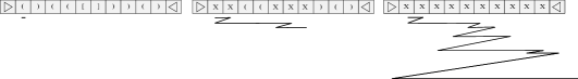
Figure 1: Some steps in an accepting computation of the automaton $M$ of Algorithm 1 on input ()(([]))().

Now we look more into the details of the implementation of this procedure, which is summarized in Algorithm 1.

1start with the head on the first input symbol

2 while symbol under the head $\neq{\mathord{\vartriangleleft}}$ do

3      move the head to the right

4       if symbol under the head $=\,\makebox[5.42494pt][c]{\footnotesize\sf)}_{i}$ (with $1\leq i\leq k$) then

5            write X

6             repeat

7                  move the head to the left

8                  

9            until symbol under the head $\neq\text{\sf X}$

10            if symbol under the head $\neq\,\makebox[5.42494pt][c]{\footnotesize\sf(}_{i}$ then Reject

11             write X

12            

13      

14 repeat

15      move the head to the left

16      

17until symbol under the head $\neq\text{\sf X}$

18if symbol under the head $={\mathord{\vartriangleright}}$ then Accept

19 else Reject

Algorithm 1 Recognition of the Dyck language $D_{k}$ 

The machine $A_{D}$ starts the computation in the initial state $q_{0}$ (line 1). While moving to the right to search for a closed bracket (line 1), $A_{D}$ does not need to keep in its finite control any other information, so it can always use the same state $q_{0}$. On the other hand, after a closed bracket $\makebox[6.02773pt][c]{\footnotesize\sf)}_{i}$ is found, $1\leq i\leq k$, $A_{D}$ needs to remember the index $i$ in order to find a matching open bracket $\makebox[6.02773pt][c]{\footnotesize\sf(}_{i}$. This is done by using a state $q_{i}$ for moving to the left while performing the search and the next rewriting (lines 1–1). The final loop and test (lines 1–1) can be performed using a further state $q_{{\mathord{\vartriangleleft}}}$. Notice that each cell containing a closed bracket is rewritten in the first visit, while changing the head direction, and each cell containing an open bracket is rewritten in the second visit. Furthermore, the content of a cell is not rewritten after the second visit. Hence the machine $A_{D}$ we just described is a deterministic ${2}$-limited automaton.  

Example 2

For each integer $n$, let us denote by $K_{n}$ the set of all strings over the alphabet $\{0,1\}$ consisting of the concatenation of blocks of length $n$, such that at least $n$ blocks are equal to the last one. Formally:

$$K_{n} = \{x_{1}x_{2}\cdots x_{k}x\mid k\geq 0,~{}x_{1},x_{2},\ldots,x_{k},x\in\{0,1\}^{n},$$

$$~{}\exists i_{1}<i_{2}<\cdots<i_{n}\in\{1,\ldots,k\},~{}x_{i_{1}}=x_{i_{2}}=\ldots=x_{i_{n}}=x\}\,.$$

We now describe a ${2}$-limited automaton $M$ accepting  $K_{n}$. Suppose $M$ receives an input string $w$ of length $N$.

1. First, $M$ scans the input tape from left to right, to reach the right end-marker.

2. $M$ moves its head $n+1$ positions to the left, namely to the cell $i=N-n$, the one immediately to the left of the input suffix $x$ of length $n$.

3. Starting from this position $i$, $M$ counts how many blocks of length $n$ coincide with $x$. This is done as follows.

   When $M$, arriving from the right, visits a position $i\leq N-n$ for the first time, it replaces the content $a$ by a special symbol $X$, after copying $a$ in the finite control. Hence, $M$ starts to move to the right, in order to compare the symbol removed from the cell with the corresponding symbol in the block $x$. While moving to the right, $M$ counts modulo $n$ and stops when the counter is $0$ and a cell containing a symbol other than $X$ is reached. The symbol of $x$ in this cell has to be compared with $a$. Then, $M$ moves to the left until it reaches cell $i-1$, namely the first cell which does not contain $X$, immediately to the left of cells containing $X$.

   We observe that the end of a block is reached each time a symbol $a$ copied from the tape is compared with the leftmost symbol of $x$, which lies immediately to the right of a cell containing $X$. If in the block just inspected no mismatches have been discovered then the counter of blocks matching with $x$ is incremented (unless its value was already $n$).

4. When the left end-marker is reached, $M$ accepts if and only if the input length is a multiple of $n$ and the counter of blocks matching with $x$ contains $n$.

We can easily observe that the above strategy can modify tape cells only in the first two visits. Hence, it can be implemented by a deterministic ${2}$-limited automaton. Such an automaton uses $O(n^{2})$ states and a constant size alphabet.

Actually, using nondeterminism, it is possible to recognize the language $K_{n}$ using $O(n)$ states and modifying tape cells only in the first visit, namely $K_{n}$ is accepted by a nondeterministic ${1}$-limited automaton $M$, which we now describe. $M$ works in three phases.

1. First, $M$ scans its tape from left to right. During this phase, $M$ marks exactly $n+1$ input cells. The first $n$ marked cells are guessed to be the leftmost positions of the $n$ input blocks $x_{i_{1}},\ldots,x_{i_{n}}$ which are expected to be equal to the rightmost block. The last marked cell is guessed to be the leftmost position of the rightmost block. This phase can be implemented using $n+2$ states, to count how many positions have been marked.

2. When the right end-marker is reached, $M$ makes a complete scan of the input from right to left, in order to verify whether or not the input length is a multiple of $n$, the last cell that has been marked in the first phase is the leftmost cell of the last block, and the other marked cells are the leftmost cells of some blocks. If the outcome of this phase is negative, then $M$ stops and rejects. The number of states used here is $2n$.

3. Finally, $M$ verifies that all the blocks starting from the marked positions contain the same string of length $n$. To this aim, the block from position $j_{h-1}$ is compared symbol by symbol with the block from position $j_{h}$, for $h=1,\ldots,n$, where $j_{0}<j_{1}<\cdots<j_{n}$ are the marked positions. To make these comparisons, $M$ with the head on the $i$th symbol of the block ${h-1}$ moves the head to the $i$th symbol of the block $h$. To detect the position of such symbol, $M$ while moving the head to the right counts modulo $n$, until, after visiting a marked cell (namely cell $j_{h}$), the value of the counter becomes $0$. If the comparison fails, then $M$ can reject, otherwise $M$ starts to move to the left, still counting modulo $n$, and searching the leftmost cell of the block $h-1$. Then $M$ can start to move to the right, while decrementing the counter, reaching cell $i$ when the counter is $0$ and so locating cell $i+1$ to start the next comparison. Furthermore, the value of the counter also allows the discovery of whether all $n$ symbols of the block have been inspected. The implementation of this phase uses $O(n)$ states.  

Computational power

The following theorem summarizes the most important known results on the computational power of $d$-limited automata:

Theorem 3

1. For each $d\geq 0$, the class of languages accepted by ${d}$-limited automata coincides with the class of context-free languages [8].

2. The class of languages accepted by deterministic ${2}$-limited automata coincides with the class of deterministic context-free languages [23].

3. For each $d\geq 2$, there exists a language which is accepted by a deterministic ${d}$-limited automaton, which cannot be accepted by any deterministic ${(d-1)}$-limited automaton [8].

4. The class of languages accepted by ${1}$-limited automata coincides with the class of regular languages [29].

The argument used by Hibbard to prove Theorem 3(i) is very difficult. He provided some constructions to transform a kind of rewriting system, equivalent to pushdown automata, to ${2}$-limited automata and vice versa, together with reductions from ${(d+1)}$-limited automata to ${d}$-limited automata, for $d\geq 2$ [8].

We now discuss a construction of ${2}$-limited automata from context-free languages (already presented in [22]), which is based on the Chomsky-Schützenberger representation theorem for context-free languages [2]. We remind the reader that this theorem states that each context-free language can be obtained by selecting in a Dyck language $D_{k}$, with $k$ kinds of brackets, only the strings belonging to a regular language $R$, and then renaming the symbols in the remaining strings according to a homomorphism $L$. More precisely, every context-free language $L\subseteq\Sigma^{*}$ can be expressed as $L=h(D_{k}\cap R)$, where $D_{k}\subseteq\Omega_{k}^{*}$, $k\geq 1$, is a Dyck language, $R\subseteq\Omega_{k}^{*}$ is a regular language, and $h:\Omega_{k}\rightarrow\Sigma^{*}$ is a homomorphism.

Hence, given $L\subseteq\Sigma^{*}$ context-free, we can consider the following machines:

• A nondeterministic transducer $T$ computing $h^{-1}$.

• The ${2}$-limited automaton $A_{D}$ described in Example 1 recognizing the Dyck language $D_{k}$.

• A finite automaton $A_{R}$ accepting the regular language $R$.

To decide if a string $w\in\Sigma^{*}$, we can combine these machines as in Figure 2.

Figure 2: A machine accepting $L=h(D_{k}\cap R)$

Now, we discuss how to embed the transducer $T$, the ${2}$-limited automaton $A_{D}$, and the automaton $A_{R}$ in a unique ${2}$-limited automaton $M$, provided that the homomorphism $h$ is non-erasing, namely $h(\sigma)\neq\epsilon$, for each $\sigma\in\Omega_{k}$.

In a first phase, $T$ and $A_{D}$ work together using a producer–consumer scheme and, after that, in a second phase $A_{R}$ is simulated. In the first phase, when $A_{D}$ has to examine for the first time a tape cell, $T$ produces in a nondeterministic way a symbol $\sigma\in h^{-1}(u)$, for a nondeterministically chosen prefix $u$ of the part of the input $w$ which starts from $T$’s current head position. Then, a move of $A_{D}$ which rewrites $\sigma$ by a new symbol $\sigma^{\prime}$ is simulated. The symbol $\sigma^{\prime}$ needs to be stored somewhere in the case $A_{D}$ has to visit the same tape cell during the computation. Furthermore, the symbol $\sigma$ will be used for the simulation of $A_{R}$. Hence, the machine $M$ has to keep both symbols $\sigma$ and $\sigma^{\prime}$. Since $h$ is non-erasing, this can be done by replacing $u$ by the pair $(\sigma,\sigma^{\prime})$ on the tape. More precisely, the tape of ${2}$-limited automaton $M$ is divided in two tracks. At the beginning of the computation, the first track contains the input $w$, while the second track is empty. In the first phase, the finite control of $M$ simulates the controls of both $T$ and $A_{D}$. $M$ alternates the simulation of some computation steps of $T$ with the simulation of some computation steps of $A_{D}$ as follows:

1. When the head reaches a cell which has not yet been visited (hence, also at the beginning of the computation), $M$ simulates $T$, by nondeterministically replacing a prefix $u$ of the remaining input, with a string $\sharp^{|u|-1}\sigma$ such that $\sigma\in h^{-1}(u)$. The symbol $\sharp$ is used for padding purposes. All the cells containing this symbol will be skipped in the future steps.

2. In the last step of the above-described part of computation, when the rightmost symbol of $u$ is replaced by $\sigma$ on the first track, $M$ also resumes the simulation of $A_{D}$, starting from a step reading $\sigma$. Hence, while writing $\sigma$ on the first track, $M$ also writes on the second track the symbol $\sigma^{\prime}$ which is produced by $A_{D}$, while rewriting $\sigma$ in the first visit.

3. If $A_{D}$ moves to the left, going back to already-visited cells, then $M$ simulates directly the moves of $A_{D}$, skipping all cells containing $\sharp$, and using the second track of the tape. When, moving to the right, the head of $M$ reaches a cell which has not been visited before, the simulation of $A_{D}$ is interrupted. (A cell not visited before can be located since it does not contain $\sharp$ and the second track is empty.) In this case, $M$ resumes the simulation of $T$, as explained at point 1, except in the case the cell contains the right end-marker.

4. When the right end-marker is reached, the first track contains a string $z\in h^{-1}(w)$, while the second track contains the result of the rewriting of $z$ by $A_{D}$ (ignoring all the cells containing $\sharp$). If $A_{D}$ rejects, namely, $z\notin D_{k}$, then $M$ rejects. Otherwise, $M$ moves its head to the left end-marker and, starting from the first tape cell, it simulates the automaton $A_{R}$, consulting the first track, in order to decide whether or not $z\in R$. Finally, $M$ accepts if and only if $A_{R}$ accepts.

Actually, the simulation of the automaton $A_{R}$ can be done in the first phase, while simulating $T$ and $A_{D}$. In particular, at the previous point 2, when $T$ produces a symbol $\sigma$ and $M$ simulates a move of $A_{D}$ on $\sigma$, $M$ can also simulate a move of $A_{R}$ on $\sigma$. To this aim, $M$ has to keep in its finite state control, together with the controls of $T$ and $A_{D}$, also the control of $A_{R}$. This increases the number of the states of $M$, but makes superfluous having the first track to keep the string $z$. Hence, it reduces the size of the working alphabet of $M$.

In this construction, we used the hypothesis that the homomorphism $h$ is non-erasing. Actually, the classical proof of the Chomsky-Schützenberger representation theorem produces an erasing homomorphism. However, an interesting variant of the theorem, recently obtained by Okhotin, states that for $L\subseteq\Sigma^{*}\setminus\Sigma$ we can always restrict ourselves to non-erasing homomorphisms, namely, we can consider $h:\Omega_{k}\rightarrow\Sigma^{+}$ [18].

We point out that the construction of ${2}$-limited automata we just outlined always produces a nondeterministic machine, since the transducer $T$ is intrinsically nondeterministic.

Actually, the transformation from pushdown automata to ${2}$-limited automaton provided by Hibbard preserves the determinism. Hence, each deterministic context-free language is accepted by a deterministic ${2}$-limited automaton. The converse inclusion, which was left open by Hibbard, has been recently proved, thus obtaining that the class of languages accepted by deterministic ${2}$-limited automata coincides with the class of deterministic context-free languages (Theorem 3(ii)) [23].

It is natural to ask what is the power of determinism in the case of ${d}$-limited automata, with $d\geq 3$. It is not difficult to describe a deterministic ${3}$-limited automaton accepting the nondeterministic context-free language $\{a^{n}b^{n}c\mid n\geq 0\}\cup\{a^{n}b^{2n}d\mid n\geq 0\}$. Indeed, Hibbard showed the existence of an infinite deterministic hierarchy (Theorem 3(iii)).

The simulation of ${1}$-limited automata by finite automata (Theorem 3(iv)) has been obtained in [29, Thm. 12.1] by adapting standard techniques involving transition tables. These techniques have been introduced for converting two-way automata into equivalent one-way automata [24].

Descriptional power

Descriptional complexity aspects related to the results in Theorem 3 have been recently investigated providing new conversions between ${2}$-limited automata and pushdown automata and between ${1}$-limited automata and finite automata.

Theorem 4 ([23])

• Each $n$-state ${2}$-limited automaton can be simulated by a pushdown automaton of size exponential in a polynomial in $n$.

• The previous upper bound becomes a double exponential when a deterministic ${2}$-limited automaton is simulated by a deterministic pushdown automaton, however it remains a single exponential if the input of the deterministic pushdown automaton is given with a symbol to mark the right end.

• Each pushdown automaton $M$ can be simulated by a ${2}$-limited automaton whose size is polynomial with respect to the size of $M$.

• The previous upper bound remains polynomial when a deterministic pushdown automaton is simulated by a deterministic ${2}$-limited automaton.

The exponential gap for the conversion of ${2}$-limited automata into equivalent pushdown automata cannot be reduced. In fact, the language $K_{n}$ presented in Example 2 is accepted by a (deterministic) ${2}$-limited automaton with $O(n^{2})$ states and a constant size alphabet, while the size of each pushdown automaton accepting it must be at least exponential in $n$ [23]. This also implies that the simulation of deterministic ${2}$-limited automata by deterministic pushdown automata is exponential in size. Actually, we conjecture that this simulation costs a double exponential, namely it matches the upper bound in Theorem 4(ii).

Theorem 5 ([22])

Each $n$-state ${1}$-limited automaton $M$ can be simulated by a nondeterministic automaton with $n\cdot 2^{n^{2}}$ states and by a deterministic automaton with $2^{n\cdot 2^{n^{2}}}$ states. Furthermore, if $M$ is deterministic then an equivalent 1dfa with no more than $n\cdot(n+1)^{n}$ states can be obtained.

The doubly exponential upper bound for the conversion of nondeterministic ${1}$-limited automata into deterministic automata is related to a double role of nondeterminism in ${1}$-limited automata. When a ${1}$-limited automaton visits one cell after the first rewriting, the possible nondeterministic transitions depend on the symbol that has been written in the cell in the first visit, which, in turns, depends on the nondeterministic choice taken in the first visit. This double exponential cannot be avoided. In fact, as we already observed, the language $K_{n}$ of Example 2 is accepted by a nondeterministic ${1}$-limited automaton with $O(n)$ states and, using standard distinguishability arguments, it can be shown that each deterministic automaton accepting it requires a number of states doubly exponential in $n$. As observed in [22], even the simulation of deterministic ${1}$-limited automata by two-way nondeterministic automata is exponential in size.

It should be interesting to investigate the size costs of the simulations of ${d}$-limited automata by pushdown automata for $d\geq 0$.

We conclude this section by briefly mentioning the case of unary languages. It is well-known that in this case each context-free language is regular [4]. Hence, for each $d\geq 0$, ${d}$-limited automata with a one letter input alphabet recognize only regular languages. In [22], a result comparing the size of unary ${1}$-limited automata with the size of equivalent two-way nondeterministic finite automata has been obtained. Quite recently, Kutrib and Wendlandt proved state lower bounds for the simulation of unary ${d}$-limited automata by different variants of finite automata [12].

3 Strongly Limited Automata

In Section 2, using the Chomsky-Schützenberger representation theorem for context-free languages, we discussed how to construct a ${2}$-limited automaton accepting a given context-free language. The main component of such an automaton is a ${2}$-limited automaton accepting a Dyck language $D_{k}$. However, Algorithm 1 described in Example 1 recognizes $D_{k}$ without fully using the capabilities of 2-limited automata. For instance, it does not need to rewrite each tape cell two times. So, we can ask if it is further possible to restrict the moves of 2-limited automata, still keeping the same computational power.

In [21] we gave a positive answer to this question, by introducing strongly limited automata, a restriction of limited automata which closely imitates the moves which are used in Algorithm 1. In particular, these machines satisfy the following restrictions:

• While moving to the right, a strongly limited automaton always uses the same state $q_{0}$ until the content of a cell (which has not been yet rewritten) is modified. Then it starts to move to the left.

• While moving to the left, the automaton rewrites each cell it meets that is not yet rewritten up to some position where it starts again to move to the right. Furthermore, while moving to the left the automaton does not change its internal state.

• In the final phase of the computation, the automaton inspects all tape cells, to check whether or not the final content belongs to a given 2-strictly locally testable language. Roughly, this means that all the factors of two letters of the string which is finally written on the tape should belong to a given set.

We now present the detailed definition of this model and then we discuss it.

Definition 1

A strongly limited automaton is a tuple ${\mathcal{M}}=(Q,\Sigma,\Gamma,\delta,q_{0},q_{{\mathord{\vartriangleright}}})$, where:

• $Q$ is a finite set of states, which is partitioned in the three disjoint sets $\{q_{0}\}$, $Q_{L}$, and $Q_{\Upsilon}$.

• $\Sigma$ and $\Gamma$ are two finite and disjoint sets of symbols, called respectively the input alphabet and the working alphabet of ${\mathcal{M}}$. Let us denote by $\Upsilon$ the global alphabet of ${\mathcal{M}}$ defined as $\Upsilon=\Sigma\cup\Gamma\cup\{{\mathord{\vartriangleright}},{\mathord{\vartriangleleft}}\}$, where ${\mathord{\vartriangleright}},{\mathord{\vartriangleleft}}\notin\Sigma\cup\Gamma$ are, respectively, the left and the right end-marker.

• $\delta:Q\times\Upsilon\rightarrow 2^{\mbox{\scalebox{0.76}{$\{\mathrel{\scalebox{1.0}[0.9]{$\dashleftarrow$}},\mathrel{\scalebox{1.0}[0.9]{$\dashrightarrow$}},\mathrel{\mathrel{\vbox{\offinterlineskip\halign{\hfil#\hfil\cr$\scriptstyle\,\text{\sf X}$\cr\kern 1.0pt\cr$\longleftarrow$\cr}}}},\mathrel{{}_{q}\!\!\mathrel{\vbox{\offinterlineskip\halign{\hfil#\hfil\cr$\scriptstyle~{}\,\text{\sf X}$\cr$\scalebox{1.6}[0.9]{$\hookleftarrow$}$\cr}}}},\mathrel{\mathrel{\vbox{\offinterlineskip\halign{\hfil#\hfil\cr$\scriptstyle\text{\sf X}~{}$\cr$\scalebox{1.6}[0.9]{$\hookrightarrow$}$\cr}}}\!\!_{\!q}},\mathrel{{}_{q\,}\!\!\reflectbox{\scalebox{1.6}[0.9]{$\mapsto$}}}\mid\text{\sf X}\in\Gamma,q\in Q\}$}}}$ is the transition function, which associates a set of possible operations with each configuration of ${\mathcal{M}}$.

• $q_{0}$ is the initial state.

• $q_{{\mathord{\vartriangleright}}}\in Q_{\Upsilon}$ is the final state.

The transition function $\delta$ has to satisfy the conditions listed below.

• For the state $q_{0}$:

  • $\delta(q_{0},a)=\{\mathrel{\scalebox{1.0}[0.9]{$\dashrightarrow$}}\}$ if $a\in\Gamma$,

  • $\delta(q_{0},a)\subseteq\{\mathrel{\scalebox{1.0}[0.9]{$\dashrightarrow$}}\}\cup\{\mathrel{{}_{q}\!\!\mathrel{\vbox{\offinterlineskip\halign{\hfil#\hfil\cr$\scriptstyle~{}\,\text{\sf X}$\cr$\scalebox{1.6}[0.9]{$\hookleftarrow$}$\cr}}}}\mid q\in Q_{L},\text{\sf X}\in\Gamma\}$ if $a\in\Sigma$,

  • $\delta(q_{0},{\mathord{\vartriangleleft}})=\{\mathrel{{}_{q_{{\mathord{\vartriangleleft}}}}\!\!\reflectbox{\scalebox{1.6}[0.9]{$\mapsto$}}}\}$,

  • $\delta(q_{0},{\mathord{\vartriangleright}})$ is undefined.

• For each state $q\in Q_{L}$:

  • $\delta(q,a)=\{\mathrel{\scalebox{1.0}[0.9]{$\dashleftarrow$}}\}$ if $a\in\Gamma$,

  • $\delta(q,a)\subseteq\{\mathrel{\mathrel{\vbox{\offinterlineskip\halign{\hfil#\hfil\cr$\scriptstyle\,\text{\sf X}$\cr\kern 1.0pt\cr$\longleftarrow$\cr}}}},\mathrel{\mathrel{\vbox{\offinterlineskip\halign{\hfil#\hfil\cr$\scriptstyle\text{\sf X}~{}$\cr$\scalebox{1.6}[0.9]{$\hookrightarrow$}$\cr}}}\!\!_{\!q_{0}}}\mid\text{\sf X}\in\Gamma\}$ if $a\in\Sigma$,

  • $\delta(q,a)$ is undefined if $a\in\{{\mathord{\vartriangleright}},{\mathord{\vartriangleleft}}\}$.

• For each state $q_{\text{\sf X}}\in Q_{\Upsilon}$:

  • $\delta(q_{\text{\sf X}},a)\subseteq\{\mathrel{{}_{q_{a}}\!\!\reflectbox{\scalebox{1.6}[0.9]{$\mapsto$}}}\}$, where $a\in\Upsilon$.

We now describe how $\mathcal{M}$ works, providing an informal explanation of the meaning of the states and of the operations that $\mathcal{M}$ can perform. First of all, we assume that at the beginning of the computation the tape contains the input string $w\in\Sigma^{*}$ surrounded by the two end-markers. Tape cells are counted from $0$. Hence, cell $0$ contains ${\mathord{\vartriangleright}}$ and cell $|w|+1$ contains ${\mathord{\vartriangleleft}}$. The head is on cell $1$, namely scanning the leftmost symbol of $w$, while the finite control is in $q_{0}$.

The initial state $q_{0}$ is the only state which is used while moving from left to right. In this state all the cells that have been already rewritten are ignored, just moving one position further, while on all the other cells $\mathcal{M}$ could be allowed either to move to the right or to rewrite the cell content and then turn the head direction to the left, entering a state in the set $Q_{L}$. To this aim, in the state $q_{0}$ the following operations could be possible:

• Move to the right $\mathrel{\scalebox{1.0}[0.9]{$\dashrightarrow$}}$
  Move the head one position to the right without rewriting the cell content and without changing the state.

• Turn to the left $\mathrel{{}_{q}\!\!\mathrel{\vbox{\offinterlineskip\halign{\hfil#\hfil\cr$\scriptstyle~{}\,\text{\sf X}$\cr$\scalebox{1.6}[0.9]{$\hookleftarrow$}$\cr}}}}$
  Write $\text{\sf X}\in\Gamma$ in the currently scanned tape cell, move one position to the left, entering in state $q\in Q_{L}$. After a sequence of moves from left to right, with this operation $\mathcal{M}$ rewrites the content of the current cell and changes the head direction, entering a state $q\in Q_{L}$.

We point out that these two operations are not allowed in states other than $q_{0}$. One further operation ($\mathrel{{}_{q_{{\mathord{\vartriangleleft}}}}\!\!\reflectbox{\scalebox{1.6}[0.9]{$\mapsto$}}}$, described later) is possible in $q_{0}$, when the right end-marker is reached, to activate the final phase of the computation.

The states in the set $Q_{L}$ are used to move to the left. In a state $q\in Q_{L}$, the automaton $\mathcal{M}$ ignores all the cells that have been already rewritten, just moving to the left. On the remaining cells that $\mathcal{M}$ visits, it always rewrites the content up to some position where it turns its head to the right. During this procedure, $\mathcal{M}$ changes state only at the end, when it enters again in $q_{0}$. In a state $q\in Q_{L}$ the following operations can be allowed:

• Move to the left $\mathrel{\scalebox{1.0}[0.9]{$\dashleftarrow$}}$
  Move the head one position to the left without rewriting the cell content and without changing the state. This move is used only on cells that have been rewritten.

• Write and move to the left $\mathrel{\mathrel{\vbox{\offinterlineskip\halign{\hfil#\hfil\cr$\scriptstyle\,\text{\sf X}$\cr\kern 1.0pt\cr$\longleftarrow$\cr}}}}$
  Write $\text{\sf X}\in\Gamma$ in the currently scanned tape cell, move one position to the left, without changing the state. This move can be used only on cells not yet rewritten.

• Turn to the right $\mathrel{\mathrel{\vbox{\offinterlineskip\halign{\hfil#\hfil\cr$\scriptstyle\text{\sf X}~{}$\cr$\scalebox{1.6}[0.9]{$\hookrightarrow$}$\cr}}}\!\!_{\!q_{0}}}$
  Write $\text{\sf X}\in\Gamma$ in the currently scanned tape cell, move one position to the right, entering in the state $q_{0}$. Even this move can be used only on cells not yet rewritten.

If the left end-marker is reached while scanning to the left in a state of $Q_{L}$ then the computation stops by rejecting (technically the next transition is undefined). On the other hand, if the right end-marker is reached while scanning to the right in $q_{0}$, the machine starts a final phase where it completely scans the tape from right to left and then stops. During the last phase $\mathcal{M}$ checks the membership of the final tape content to a local language. If some forbidden factor is detected then the next transition is undefined and hence $\mathcal{M}$ rejects. To this aim, in this phase only states from the set $Q_{\Upsilon}$ are used. We assume that there is a surjective map from $\Upsilon$ to $Q_{\Upsilon}$. We simply denote as $q_{\text{\sf X}}$ the state associated with the symbol $\text{\sf X}\in\Upsilon$. Note that $\text{\sf X}\neq\text{\sf Y}$ does not implies $q_{\text{\sf X}}\neq q_{\text{\sf Y}}$. The following operation is used in this phase:

• Check to the left $\mathrel{{}_{q_{a}}\!\!\reflectbox{\scalebox{1.6}[0.9]{$\mapsto$}}}$
  On a cell containing symbol $a\in\Upsilon$, move to the left remembering the state associated with $a$.

If no forbidden factor is found, $\mathcal{M}$ finally violates the left end-marker in the state $q_{{\mathord{\vartriangleright}}}$. In this case the input is accepted. Otherwise the computation of $\mathcal{M}$ stopped in some previous step, rejecting the input. Hence, we assume that $\mathcal{M}$ accepts its input if and only if from the cell containing the left end-marker it can further move to the left entering the final state $q_{{\mathord{\vartriangleright}}}$.

Example 6

Consider the alphabet $\Omega_{2}$, with brackets represented by the symbols $\makebox[6.02773pt][c]{\footnotesize\sf(},\makebox[6.02773pt][c]{\footnotesize\sf)},\makebox[6.02773pt][c]{\footnotesize\sf[},\makebox[6.02773pt][c]{\footnotesize\sf]}$. The Dyck language $D_{2}$ is accepted by a strongly limited automaton with $\Gamma=\{\text{\sf X}\}$, $Q_{L}=\{q_{1},q_{2}\}$, $Q_{\Upsilon}=\{q_{\text{\sf X}},q_{{\mathord{\vartriangleright}}},q_{{\mathord{\vartriangleleft}}}\}$, and the following transitions (we omit braces for the sake of the brevity):

• $\delta(q_{0},\makebox[6.02773pt][c]{\footnotesize\sf(})=\delta(q_{0},\makebox[6.02773pt][c]{\footnotesize\sf[})=\,\mathrel{\scalebox{1.0}[0.9]{$\dashrightarrow$}}$, $\delta(q_{0},\makebox[6.02773pt][c]{\footnotesize\sf)})=\,\mathrel{{}_{q_{1}}\!\!\mathrel{\vbox{\offinterlineskip\halign{\hfil#\hfil\cr$\scriptstyle~{}\,\text{\sf X}$\cr$\scalebox{1.6}[0.9]{$\hookleftarrow$}$\cr}}}}$, $\delta(q_{0},\makebox[6.02773pt][c]{\footnotesize\sf]})=\,\mathrel{{}_{q_{2}}\!\!\mathrel{\vbox{\offinterlineskip\halign{\hfil#\hfil\cr$\scriptstyle~{}\,\text{\sf X}$\cr$\scalebox{1.6}[0.9]{$\hookleftarrow$}$\cr}}}}$,

• $\delta(q_{1},\text{\sf X})=\delta(q_{2},\text{\sf X})=\,\mathrel{\scalebox{1.0}[0.9]{$\dashleftarrow$}}$, $\delta(q_{1},\makebox[6.02773pt][c]{\footnotesize\sf(})=\delta(q_{2},\makebox[6.02773pt][c]{\footnotesize\sf[})=\,\mathrel{\mathrel{\vbox{\offinterlineskip\halign{\hfil#\hfil\cr$\scriptstyle\text{\sf X}~{}$\cr$\scalebox{1.6}[0.9]{$\hookrightarrow$}$\cr}}}\!\!_{\!q_{0}}}$,

• $\delta(q_{0},{\mathord{\vartriangleleft}})=\,\mathrel{{}_{q_{{\mathord{\vartriangleleft}}}}\!\!\reflectbox{\scalebox{1.6}[0.9]{$\mapsto$}}}$, $\delta(q_{{\mathord{\vartriangleleft}}},\text{\sf X})=\delta(q_{\text{\sf X}},\text{\sf X})=\,\mathrel{{}_{q_{\text{\sf X}}}\!\!\reflectbox{\scalebox{1.6}[0.9]{$\mapsto$}}}$, $\delta(q_{\text{\sf X}},{\mathord{\vartriangleright}})=\,\mathrel{{}_{q_{{\mathord{\vartriangleright}}}}\!\!\reflectbox{\scalebox{1.6}[0.9]{$\mapsto$}}}$.

It can be observed that the states $q_{{\mathord{\vartriangleleft}}},q_{\text{\sf X}},q_{{\mathord{\vartriangleright}}}$, used in the final scan, can be merged in a unique state $q_{{\mathord{\vartriangleright}}}$. In fact, in this example the purpose of the final scan is to check that all the input symbols have been rewritten, namely, no symbol $a\in\{\makebox[6.02773pt][c]{\footnotesize\sf(},\makebox[6.02773pt][c]{\footnotesize\sf)},\makebox[6.02773pt][c]{\footnotesize\sf[},\makebox[6.02773pt][c]{\footnotesize\sf]}\}$ is left on the tape. If such a symbol is discovered, then the next transition is not defined and hence the computation rejects.  

Example 7

The deterministic context-free language $\{a^{n}b^{2n}\mid n\geq 0\}$ is accepted by a strongly limited automaton which guesses each second $b$. While moving from left to right and reading $b$, the automaton makes a nondeterministic choice between further moving to the right or rewriting the cell by X and turning to the left. Furthermore, while moving to the left, the content of each cell containing $b$ which is visited is rewritten by Y, still moving to the left, and when a cell containing $a$ is visited, its content is replaced by Z, turning to the right. In the final scan the machine accepts if and only if the string on the tape belongs to ${\mathord{\vartriangleright}}\text{\sf Z}^{*}(\text{\sf Y}\text{\sf X})^{*}{\mathord{\vartriangleleft}}$.

We can modify the above algorithm to recognize the language $\{a^{n}b^{n}\mid n\geq 0\}\cup\{a^{n}b^{2n}\mid n\geq 0\}$. While moving from left to right, when the head reaches a cell containing $b$ three actions are possible: either the automaton continues to move to the right, without any rewriting, or it rewrites the cell by Z, turning to the right, or it rewrites the cell by W, also turning to the right. While moving from right to left, the automaton behaves as the one above described for $\{a^{n}b^{2n}\mid n\geq 0\}$. The input is accepted if and only if the string which is finally on the tape belongs to ${\mathord{\vartriangleright}}\text{\sf Z}^{*}\text{\sf W}^{*}{\mathord{\vartriangleleft}}+{\mathord{\vartriangleright}}\text{\sf Z}^{*}(\text{\sf Y}\text{\sf X})^{*}{\mathord{\vartriangleleft}}$.  

We already mentioned that strongly limited automata have the same computational power as limited automata, namely they characterize context-free languages. This result has been proved in [21], also studying descriptional complexity aspects:

Theorem 8 ([21])

• Each context-free language $L$ is accepted by a strongly limited automaton whose description has a size which is polynomial with respect to the size of a given context-free grammar generating $L$ or of a given pushdown automaton accepting $L$.

• Each strongly limited automaton $\mathcal{M}$ can be simulated by a pushdown automaton of size polynomial with respect the size of $\mathcal{M}$.

The proof of (i) was obtained using a further variant of the Chomsky-Schützenberger representation theorem, also proved by Okhotin [18]. In this variant Dyck languages extended with neutral symbols and letter-to-letter homomorphisms are used. (ii) has been proved by providing a direct simulation.

Concerning deterministic computations, it is not difficult to observe that deterministic strongly limited automata cannot recognize all deterministic context-free languages. Consider, for instance, the deterministic language $L=\{ca^{n}b^{n}\mid n\geq 0\}\cup\{da^{2n}b^{n}\mid n\geq 0\}$. While moving from left to right, a strongly limited automaton can use only the state $q_{0}$. Hence, it cannot remember if the first symbol of the input is a $c$ or a $d$ and, then, if it has to check whether the number of $a$s is equal to the number of $b$s or whether the number of $a$s is two times the number of $b$s. A formal proof that the language $L$, and also the language $\{a^{n}b^{2n}\mid n\geq 0\}$ (Example 7), are not accepted by any deterministic strongly limited automaton is presented in [21].

In that paper it was also proposed to slightly relax the definition of strongly limited automata, by introducing a set of states $Q_{R}$, with $q_{0}\in Q_{R}$, used while moving to the right, and allowing transitions between states of $Q_{L}$ and of $Q_{R}$ while moving to the left and to the right, respectively, but still forbidding state changes on rewritten cells and by keeping all the other restrictions. This model, called almost strongly limited automata, still characterizes the context-free languages. Furthermore, the two deterministic context-free languages mentioned in the previous paragraph can be easily recognized by almost strongly limited automata having only deterministic transitions.

It would be interesting to know if almost strongly limited automata are able to accept all deterministic context-free languages without taking nondeterministic decisions.

4 Conclusion

We discussed some restricted versions of one-tape Turing machines characterizing context-free languages. Some other interesting models are presented in the literature. We briefly mention some of them.

In 1996 Jancar, Mráz, and Plátek introduced forgetting automata [10]. These devices can erase tape cells by rewriting their contents with a special symbol. However, rewritten cells are kept on the tape and are still considered during the computation. For instance, the state can be changed while visiting an erased cell. In a variant of forgetting automata that characterizes context-free languages, when a cell which contains an input symbol is visited while moving to the left, its content is rewritten, while no changes can be done while moving to the right. This way of operating is very close to that of strongly limited automata. However, in strongly limited automata the rewriting alphabet can contain more than one symbol. Furthermore, rewritten cells are completely ignored (namely, the head direction and the state cannot be changed while visiting them) except in the final scan of the tape from the right to the left end-marker. So the two models are different. For example, to recognize the set of palindromes, a strongly limited automaton needs a working alphabet of at least $3$ symbols while, by definition, to rewrite tape cells forgetting automata use only one symbol [21].

If erased cells are removed from the tape of a forgetting automaton, we obtain another computational model called deleting automata. This model is less powerful. In fact it is not able to recognize all context-free languages [10].

Wechsung proposed another complexity measure for one-tape Turing machines called return complexity [30, 31]. This measure counts the maximum number of visits to a tape cell, starting from the first visit which modifies the cell content. It should be clear that return complexity $1$ characterizes regular languages (each cell, after the first rewriting, will be never visited again, hence the rewriting is useless). Furthermore, for each $d\geq 2$, return complexity $d$ characterizes context-free languages. Notice that this measure is dual with respect to the one considered to define limited automata. Even with respect to return complexity, there exists a hierarchy of deterministic languages (cf. Theorem 3(iii) in the case of limited automata). However, this hierarchy is not comparable with the class of deterministic context-free languages. For instance, it can be easily seen that the set of palindromes, which is not a deterministic context-free language, can be recognized by a deterministic machine with return complexity $2$. However, there are deterministic context-free languages that cannot be recognized by any deterministic machine with return complexity $d$, for any integer $d$ [19].

With the aim of investigating computations with very restricted resources, Hemaspaandra, Mukherji, and Tantau studied one-tape Turing machine with absolutely no space overhead, a model which is very close to “realistic” computations, where the space is measured without any hidden constants [6]. These machines use the binary alphabet $\Sigma=\{0,1\}$ (plus two end-marker symbols) and only the portion of the tape which at the beginning of the computation contains the input. Furthermore, no other symbols are available, namely only symbols from $\Sigma$ can be used to rewrite the tape. Despite these strong restrictions, there machines are able to recognize in polynomial time all context-free languages over $\Sigma$.

Acknowledgment

Many thanks to Lane Hemaspaandra, editor of the SIGACT News Complexity Theory Column, for the careful reading of the first draft of the paper. His suggestions and recommendations were very useful for improving the quality of the paper.

References

- [1] Alberts, M.: Space complexity of alternating Turing machines. In: Budach, L. (ed.) Fundamentals of Computation Theory, FCT ’85, Cottbus, GDR, September 9-13, 1985. Lecture Notes in Computer Science, vol. 199, pp. 1–7. Springer (1985), http://dx.doi.org/10.1007/BFb0028785
- [2] Chomsky, N., Schützenberger, M.: The algebraic theory of context-free languages. In: Braffort, P., Hirschberg, D. (eds.) Computer Programming and Formal Systems, Studies in Logic and the Foundations of Mathematics, vol. 35, pp. 118–161. Elsevier (1963)
- [3] Geffert, V.: Bridging across the log(n) space frontier. Inf. Comput. 142(2), 127–158 (1998), http://dx.doi.org/10.1006/inco.1997.2682
- [4] Ginsburg, S., Rice, H.G.: Two families of languages related to ALGOL. J. ACM 9(3), 350–371 (1962), http://doi.acm.org/10.1145/321127.321132
- [5] Hartmanis, J.: Computational complexity of one-tape Turing machine computations. J. ACM 15(2), 325–339 (1968), http://doi.acm.org/10.1145/321450.321464
- [6] Hemaspaandra, L.A., Mukherji, P., Tantau, T.: Context-free languages can be accepted with absolutely no space overhead. Inf. Comput. 203(2), 163–180 (2005), http://dx.doi.org/10.1016/j.ic.2005.05.005
- [7] Hennie, F.C.: One-tape, off-line Turing machine computations. Information and Control 8(6), 553–578 (1965), http://dx.doi.org/10.1016/S0019-9958(65)90399-2
- [8] Hibbard, T.N.: A generalization of context-free determinism. Information and Control 11(1/2), 196–238 (1967), http://dx.doi.org/10.1016/S0019-9958(67)90513-X
- [9] Hopcroft, J.E., Ullman, J.D.: Some results on tape-bounded Turing machines. J. ACM 16(1), 168–177 (1969), http://doi.acm.org/10.1145/321495.321508
- [10] Jancar, P., Mráz, F., Plátek, M.: Forgetting automata and context-free languages. Acta Inf. 33(5), 409–420 (1996), http://dx.doi.org/10.1007/s002360050050
- [11] Kuroda, S.: Classes of languages and linear-bounded automata. Information and Control 7(2), 207–223 (1964), http://dx.doi.org/10.1016/S0019-9958(64)90120-2
- [12] Kutrib, M., Wendlandt, M.: On simulation cost of unary limited automata. In: Shallit, J., Okhotin, A. (eds.) Descriptional Complexity of Formal Systems - 17th International Workshop, DCFS 2015, Waterloo, ON, Canada, June 25-27, 2015. Proceedings. Lecture Notes in Computer Science, vol. 9118, pp. 153–164. Springer (2015), http://dx.doi.org/10.1007/978-3-319-19225-3_13
- [13] Lewis II, P.M., Stearns, R.E., Hartmanis, J.: Memory bounds for recognition of context-free and context-sensitive languages. In: 6th Annual Symposium on Switching Circuit Theory and Logical Design, Ann Arbor, Michigan, USA, October 6-8, 1965. pp. 191–202. IEEE (1965), http://dx.doi.org/10.1109/FOCS.1965.14
- [14] McNaughton, R., Papert, S.A.: Counter-Free Automata (M.I.T. Research Monograph No. 65). The MIT Press (1971)
- [15] Mereghetti, C.: Testing the descriptional power of small Turing machines on nonregular language acceptance. Int. J. Found. Comput. Sci. 19(4), 827–843 (2008), http://dx.doi.org/10.1142/S012905410800598X
- [16] Michel, P.: An NP-complete language accepted in linear time by a one-tape Turing machine. Theor. Comput. Sci. 85(1), 205–212 (1991), http://dx.doi.org/10.1016/0304-3975(91)90054-6
- [17] Michel, P.: A survey of space complexity. Theor. Comput. Sci. 101(1), 99–132 (1992), http://dx.doi.org/10.1016/0304-3975(92)90151-5
- [18] Okhotin, A.: Non-erasing variants of the Chomsky-Schützenberger theorem. In: Yen, H., Ibarra, O.H. (eds.) Developments in Language Theory - 16th International Conference, DLT 2012, Taipei, Taiwan, August 14-17, 2012. Proceedings, Lecture Notes in Computer Science, vol. 7410, pp. 121–129. Springer (2012), http://dx.doi.org/10.1007/978-3-642-31653-1_12
- [19] Peckel, J.: On a deterministic subclass of context-free languages. In: Gruska, J. (ed.) Mathematical Foundations of Computer Science 1977, 6th Symposium, Tatranska Lomnica, Czechoslovakia, September 5-9, 1977, Proceedings. Lecture Notes in Computer Science, vol. 53, pp. 430–434. Springer (1977), http://dx.doi.org/10.1007/3-540-08353-7_164
- [20] Pighizzini, G.: Nondeterministic one-tape off-line Turing machines. Journal of Automata, Languages and Combinatorics 14(1), 107–124 (2009)
- [21] Pighizzini, G.: Strongly limited automata. Fundam. Inform. (to appear), a preliminary version appeared in: Bensch, S., Freund, R., Otto, F. (eds.) Sixth Workshop on Non-Classical Models for Automata and Applications - NCMA 2014, Kassel, Germany, July 28-29, 2014. Proceedings. books@ocg.at, vol. 304, pp. 191–206. Österreichische Computer Gesellschaft (2014)
- [22] Pighizzini, G., Pisoni, A.: Limited automata and regular languages. Int. J. Found. Comput. Sci. 25(7), 897–916 (2014), http://dx.doi.org/10.1142/S0129054114400140
- [23] Pighizzini, G., Pisoni, A.: Limited automata and context-free languages. Fundam. Inform. 136(1-2), 157–176 (2015), http://dx.doi.org/10.3233/FI-2015-1148
- [24] Shepherdson, J.C.: The reduction of two-way automata to one-way automata. IBM J. Res. Dev. 3(2), 198 –200 (1959)
- [25] Stearns, R.E., Hartmanis, J., Lewis II, P.M.: Hierarchies of memory limited computations. In: 6th Annual Symposium on Switching Circuit Theory and Logical Design, Ann Arbor, Michigan, USA, October 6-8, 1965. pp. 179–190. IEEE (1965), http://dx.doi.org/10.1109/FOCS.1965.11
- [26] Szepietowski, A.: Turing Machines with Sublogarithmic Space, Lecture Notes in Computer Science, vol. 843. Springer (1994), http://dx.doi.org/10.1007/3-540-58355-6
- [27] Tadaki, K., Yamakami, T., Lin, J.C.H.: Theory of one-tape linear-time Turing machines. Theor. Comput. Sci. 411(1), 22–43 (2010), http://dx.doi.org/10.1016/j.tcs.2009.08.031
- [28] Trakhtenbrot, B.A.: Turing machine computations with logarithmic delay, (in russian). Algebra I Logica 3, 33–48 (1964)
- [29] Wagner, K.W., Wechsung, G.: Computational Complexity. D. Reidel Publishing Company, Dordrecht (1986)
- [30] Wechsung, G.: Characterization of some classes of context-free languages in terms of complexity classes. In: Becvár, J. (ed.) Mathematical Foundations of Computer Science 1975, 4th Symposium, Mariánské Lázne, Czechoslovakia, September 1-5, 1975, Proceedings. Lecture Notes in Computer Science, vol. 32, pp. 457–461. Springer (1975), http://dx.doi.org/10.1007/3-540-07389-2_233
- [31] Wechsung, G., Brandstädt, A.: A relation between space, return and dual return complexities. Theor. Comput. Sci. 9, 127–140 (1979), http://dx.doi.org/10.1016/0304-3975(79)90010-0